Location-aware Beam Alignment for mmWave Communications

Abstract

Beam alignment is required in millimeter wave communication to ensure high data rate transmission. However, with narrow beamwidth in massive MIMO, beam alignment could be computationally intensive due to the large number of beam pairs to be measured. In this paper, we propose an efficient beam alignment framework by exploiting the location information of the user equipment (UE) and potential reflecting points. The proposed scheme allows the UE and the base station to perform a coordinated beam search from a small set of beams within the error boundary of the location information, the selected beams are then used to guide the search of future beams. To further reduce the number of beams to be searched, we propose an intelligent search scheme within a small window of beams to determine the direction of the actual beam. The proposed beam alignment algorithm is verified on simulation with some location uncertainty.

I Introduction

Millimeter-wave (mmWave) spectrum has been proposed for the fifth generation (5G) communication networks due to the large bandwidth available at this frequency band. Other advantages such as beamforming and spatial multiplexing are leading to an increased interest in the mmWave spectrum [2]. However, the key challenge is that the mmWave spectrum suffers from severe path-loss. On the other hand, the high-frequency spectrum allows the use of a large antenna array with small form factor, which provides high beamforming gains to compensate for the losses. As such, beamforming at the base station (BS) and the user equipment (UE) have become an essential part of the mmWave 5G networks [3, 4].

Although as the number of array antenna increases, the array gain also increases with reduced interference [5], a new challenge of selecting the best beam pair at the transmitter and receiver exist due to the narrow beamwidth [6], which could compromise the transmission rate especially when the time taken for beam alignment is large [7]. Consequently, beam alignment especially in a mobile environment may become the bottleneck of the communication network. More specifically, in the initial access phase, beams with narrow beamwidth can complicate the initial cell search since the UE and BS have to search over a large angular directional space for suitable path to establish communication [8, 9].

When a user enters a cell, the user establishes a physical connection to the BS in the initial access phase. In current 4G networks, the UE regularly monitor the omnidirectional signal to estimate the downlink channel. However, in 5G mmWave networks, this is difficult to achieve due to the directionality and the rapid variations of the channel [10]. The directionality may significantly delay the initial access procedure, especially for beams with narrow beamwidth [11]. To reduce the beam alignment overhead, efficient beam alignment algorithms are therefore required. Motivated by this challenge, this paper proposes a new beam alignment algorithm which exploits a noisy location information.

Beam alignment has been previously studied under the cell search phase [12, 13, 14, 15, 16] (i.e., the phase in which the UE search and connects to a BS with a mutual agreement on transmission parameters). In [17], an exhaustive search algorithm to determine the optimal beam pair was proposed. The exhaustive search is known for its high complexity. To reduce the delay in the exhaustive search algorithm, an efficient hierarchical codebook adaptive algorithm is proposed in [18] to jointly search over the channel subspace. The proposed algorithm allows the UE and BS to jointly align their beams within a constrained time. In [19], a Bayesian tree search algorithm is proposed to reduce the delay in the training of beamforming and combining vectors.

Beam alignment overhead can be reduced without compromising performance if the location side information is available at both nodes. Indeed, 5G communication devices are expected to have access to location information which can be obtained from GNSS satellites, sensors and 5G radio signal [20, 21]. In [22], exploiting location information for backhaul systems was proposed. The authors showed that the time required for beam alignment can be reduced if the position information is shared between the nodes. For stationary backhaul systems, it is easy to assume that perfect location information is available at both nodes since this information can be obtained during installations. However, for a mobile device, it is likely that the location information is noisy and designing beam alignment algorithms might not be straightforward as in [22]. A noisy location information is considered in [23], where the authors focused on an independent beam pre-selection at the BS and the UE. While the pre-selection algorithm can improve the beam selection speed, the performance of the selected beams cannot be guaranteed since the beam selection decision is weighed on the noisy location information. In addition, the decentralized beam selection framework may degrade system performance.

This work focus on achieving fast and efficient transmit and receive beam alignment subject to a target rate constraint by exploiting the noisy location information of the UE and potential reflecting points. The location information of the static BS is assumed to be perfectly known, while the location information of the reflecting points and UE are considered to be noisy.

The contributions of this paper are summarized as follows: Firstly, we propose a beam alignment algorithm iteratively executed at the BS and the UE that exploits the location information of the UE and potential reflecting points, this information is used to design a subset of beam codebook from the BS and UE codebooks, thereby reducing the number of beam steering vectors to be searched as compared to the exhaustive search algorithm. Secondly, we propose a search window in the subset of beam codebooks to further reduce the angular space to be searched. This is achieved by determining the direction of the actual beam after obtaining the local optimal beam within the search window. Furthermore, the local optimal beam in each search is used to guide future beam search at the UE and BS thereby reducing the beam alignment overhead. Finally, we derive the Cramér-Rao bound (CRB) of the channel parameter which an unbiased estimator should satisfy, the CRB is then used to model the channel estimation error. We show by simulations that the proposed beam alignment scheme can speed up the beam alignment process and reduce the beam alignment overhead when compared to existing schemes.

The rest of the paper is organized as follows. In Section II, the signal model and the codebook used in this paper are introduced. Section III first describes the use of location information followed by a detail description of the proposed beam alignment algorithm. In Section IV, we present the channel parameter estimation and rate evaluation. Numerical results are shown in section V, and the paper is concluded in Section VI.

Notations

Throughout this paper, matrices and vector symbols are represented by uppercase and lowercase boldface respectively. $\mathbf{A}^{*}$, $\mathbf{A}^{\mathsf{T}}$ and $\mathbf{A}^{\mathsf{H}}$ represent the complex conjugate, transpose and Hermitian transpose of the matrix $\mathbf{A}$ respectively. The mathematical expectation is denoted as $\mathbb{E}[.]$. tr$(\mathbf{A})$ represent the trace of matrix $\mathbf{A}$. The Kronecker product between two matrices $\mathbf{A}$ and $\mathbf{B}$ is denoted as $\mathbf{A}\otimes\mathbf{B}$.

\psfrag{a}[bc][bc][1][0]{$[x_{\text{BS}},y_{\text{BS}}]$}\psfrag{b}[Bc][Bc][1][-40]{$\quad\quad[x_{1},y_{1}]$}\psfrag{c}[bc][bc][1][0]{$\quad[x_{2},y_{2}]$}\psfrag{d}[bc][bc][1][-38]{$[x_{\text{UE}},y_{\text{UE}}]$}\includegraphics[width=303.53267pt]{Figures/Figure1Update}

Figure 1: Example of network scenario with two reflectors

II System Model

Consider a wireless network scenario operating in the mmWave frequency band and consisting of one UE, one BS, $M$ dominant paths with one line of sight (LOS) path and $M-1$ reflected paths as shown in Fig 1. The orientation of the UE is assumed to be fixed, however, the proposed scheme can also be extended to a scenario where the orientation of the UE is not known. In such scenario, the UE’s orientation can be estimated along with the location information [24] after which the beam alignment algorithm proposed in this paper can be applied. The Cartesian coordinate of each node defines its position while the location of the BS is assumed to be known by the UE. The location information in this paper is discussed in detail in the Section III. We assume that the UE and the BS are equipped with receive and transmit uniform linear array (ULA) $N_{r}$ and $N_{t}$ antennas respectively. Furthermore, we assume the communication is made in blocks (i.e., at discrete instance), where each block consists of $N$ slots. The channel is assumed to remain constant within each block and change independently between blocks. From the $N$ slots, $N_{a}$ slots are used for the control phase within which beam alignment will be achieved, while $N-N_{a}$ slots are used for the data transmission phase. Note that the proposed beam alignment protocol requires both the uplink and downlink communication as the protocol is iteratively executed by both the BS and the UE. We assume the BS and UE are allowed to dwell in a slot with a fixed beamformer. More specifically, within each BS-slot, the BS beamformer is kept fixed and used to transmit to the UE while the UE takes several measurements with different UE beam directions. Similarly, in the UE-slot, the UE beamformer is fixed while the BS can take several measurements with different BS beam directions. We fix the number of beams that can be processed per slot as $N_{b}$. It can be observed that while data transmission can be improved by selecting the best beam pair, the number of slots $N_{a}$ taken to achieve beam alignment should be as low as possible to reduce beam alignment overhead [25, 11]. Hence, the proposed scheme aims to speed up the beam pair search subject to a rate constraint.

II-A Signal and Channel Model

In this section, we present the signal model. We assume beamforming vector $\mathbf{v}_{k}$ where $k\in\{1,2,\ldots,N_{t}\}$ is employed at the BS while the UE employs beamforming vector $\mathbf{u}_{j}$, where $j\in\{1,2,\ldots,N_{r}\}$. Furthermore, we assume the beam vectors are normalized to unity: $\|\mathbf{v}_{k}\|=\|\mathbf{u}_{j}\|=1$. The downlink received signal can be expressed as

$$y_{j,k}=\mathbf{u}_{j}^{\mathsf{H}}\mathbf{H}\mathbf{v}_{k}s+\mathbf{u}_{j}^{\mathsf{H}}\mathbf{n},$$ (1)

where $\mathbf{u}_{j}\in\mathcal{C}^{N_{r}\times 1}$ and $\mathbf{v}_{k}\in\mathcal{C}^{N_{t}\times 1}$, $s$ is the transmitted symbol with unit energy $\left|s\right|=\sqrt{E_{s}}$, $E_{s}$ is the transmit energy, $\mathbf{n}\in\mathcal{C}^{N_{r}\times 1}$ is the complex Gaussian noise vector with zero mean and covariance $\sigma^{2}\mathbf{I}$. The downlink channel $\mathbf{H}$ is expressed as [26]

$$\mathbf{H}=\sqrt{N_{t}N_{r}}\sum_{m=0}^{M-1}\alpha_{m}\mathbf{a}_{r}(\theta_{m})\mathbf{a}_{t}^{\mathsf{H}}(\phi_{m}),$$ (2)

where $M$ is the number of multi-paths, consisting of one LOS path and $M-1$ reflected paths, specifically, $m=0$ refers to the LOS path, and $m=1,\ldots,M-1$, refers to the $m$-th NLOS path passing through the $m$-th reflecting points. $\theta_{m}$ and $\phi_{m}$ are the angle of arrival (AOA) and angle of departure (AOD) of the $m$-th path at the receiver and transmitter in the downlink mode respectively, $\alpha_{m}\sim\mathcal{CN}(0,\sigma^{2}_{\alpha})$ denotes the instantaneous random complex gain for the $m$-th path. The corresponding array response vectors at the UE and BS denoted as $\mathbf{a}_{r}(\theta_{m})$ and $\mathbf{a}_{t}(\phi_{m})$ are given by

$$\mathbf{a}_{r}(\theta_{m})=\frac{1}{\sqrt{N_{r}}}\left[1,e^{-j\pi\cos\theta_{m}},\ldots,e^{-j\pi(N_{r}-1)\cos\theta_{m}}\right]^{\mathsf{T}},$$ (3)

$$\mathbf{a}_{t}(\phi_{m})=\frac{1}{\sqrt{N_{t}}}\left[1,e^{-j\pi\cos\phi_{m}},\ldots,e^{-j\pi(N_{t}-1)\cos\phi_{m}}\right]^{\mathsf{T}},$$ (4)

respectively. We assume that the steering vectors are drawn from a codebook and the design of the codebook is presented as follows.

II-B Codebook Structure

The AOD and AOA are computed from the estimated location information and are associated with transmit and receive beamforming vectors respectively from a given codebook. The focus of this paper is not the codebook design, therefore we refer our readers to [27] for details on codebook design. In this paper, the codebooks are designed to achieve approximately equal gain but with narrow beams at the broadside and wide beams at the endfire [28]. The pointing angles at the UE and BS denoted as $\bar{\theta}_{j}$ and $\bar{\phi}_{k}$ respectively are separated into grids as follows

$$\bar{\theta}_{j}=\arccos\left(1-\frac{2\left(j-1\right)}{N_{r}-1}\right),\quad j=1,\ldots,N_{r},$$ (5)

$$\bar{\phi}_{k}=\arccos\left(1-\frac{2\left(k-1\right)}{N_{t}-1}\right),\quad k=1,\ldots,N_{t},$$ (6)

where $0\leq\arccos\left(x\right)\leq\pi$. The receive and transmit codebook is defined as

$$\mathcal{U} {}={} \left[\mathbf{u}_{1},\dots,\mathbf{u}_{N_{r}}\right],$$ (7)

$$\mathcal{V}{} {}={} \left[\mathbf{v}_{1},\dots,\mathbf{v}_{N_{t}}\right],$$ (8)

where $\mathbf{u}_{j}=\mathbf{a}_{r}(\bar{\theta}_{j})$ and $\mathbf{v}_{k}=\mathbf{a}_{t}(\bar{\phi}_{k})$ are the beam steering vectors over the discrete grid angles. It can be observed from (5) and (6), that the codebook covers a large angular space. The exhaustive search requires that the BS and UE search through the entire codebook $\mathcal{U}$ and $\mathcal{V}$ respectively. The beam alignment is achieved by selecting the beam pair that maximizes the downlink rate, which can be mathematically expressed as

$$\underset{\left\{{\mathbf{u},\mathbf{v}}\right\}\in\mathcal{U}\times\mathcal{V}}{\max}R_{d}(\mathbf{u},\mathbf{v}),$$ (9)

where

$$R_{d}\left(\mathbf{u},\mathbf{v}\right)=\log_{2}\left(1+\frac{E_{s}\left|\mathbf{u}^{\mathsf{H}}\mathbf{H}\mathbf{v}\right|^{2}}{\sigma^{2}}\right).$$ (10)

Note that in (9), we assume that the channel state information is perfectly known, which enables us the know the SNR at the receiver and evaluate average rate under any choice of $\mathbf{v}$ and $\mathbf{u}$. However, performing beam alignment by exhaustive search method may incur high system overhead. In addition, due to the dynamic nature of the channel, especially in a mobile scenario this method may not be suitable for 5G communication.

Hence, we focus on achieving fast transmit and receive beam alignment subject to a target rate $R_{0}$, where $R_{0}\leq R_{d}\left(\mathbf{u},\mathbf{v}\right)$. The proposed scheme is discussed in details in the following section.

III Beam Alignment with Location Information

In this section, we focus on the proposed beam alignment algorithm. We assume that the location information of possible reflecting points can be independently estimated by the BS and the UE [24, 29]. However, we note that the location information could be erroneous, and the uncertainty of the location information at the nodes are included in the design of the proposed algorithm.

III-A Exploiting Location Information

Location information can be obtained with the use of available positioning technologies. The location information obtained at the BS and UE may be noisy due to latency in the position information exchange or due to the use of different positioning technologies at the UE and BS. For instance, the BS may be able to estimate potential reflecting points more accurately than the UE due to interactions with multiple UEs.

We define the location matrix $\mathbf{L}_{i}\in\mathbb{R}^{2\times M}$ containing the actual location coordinate of the nodes, where the nodes refer to the potential reflecting points and either the BS or UE. Specifically, when the location information is estimated from the BS, the location information matrix contains the coordinate information of the UE and the reflecting points. Similarly, when the location information is measured from the UE, the location information matrix contains the coordinate information of the BS and the reflecting points. Hence, we express $\mathbf{L}_{i}$ as follows

$$\mathbf{L}_{i}=\left[\mathbf{l}_{0},\mathbf{l}_{1},\ldots,\mathbf{l}_{{M-1}}\right],\quad$$ (11)

where

$$\mathbf{l}_{0}=\begin{cases}\mathbf{l}_{\text{BS}}\quad\text{for }i=\text{UE},\\ \mathbf{l}_{\text{UE}}\quad\text{for }i=\text{BS},\end{cases}$$ (12)

and $\mathbf{l}_{m}=[x_{m},y_{m}]^{\mathsf{T}}$ is the location information of the node along path $m$. The location information of the observer is denoted as $\mathbf{l}_{\text{BS}}$ for the BS and $\mathbf{l}_{\text{UE}}$ for the UE. Note from (11) that when the UE is the observer, $\mathbf{l}_{0}=\mathbf{l}_{\text{BS}}$, and when the BS is the observer, $\mathbf{l}_{0}=\mathbf{l}_{\text{UE}}$. Furthermore, we model the independent location information of the UE and $M-1$ reflecting points available at the BS as

$$\hat{\mathbf{L}}_{\text{BS}}=\mathbf{L}_{\text{BS}}+\mathbf{E}_{\text{BS}},$$ (13)

where $\mathbf{E}_{\text{BS}}$ is the matrices containing the random location estimation errors of the $x$ and $y$ coordinates made by the BS given as

$$\mathbf{E}_{\text{BS}}=[\mathbf{e}_{0}^{\text{BS}},\mathbf{e}_{1}^{\text{BS}},\ldots,\mathbf{e}_{{M-1}}^{\text{BS}}],$$ (14)

where the superscript BS and UE are used to indicate the observation at the BS and UE respectively. In this paper, we adopt a uniform bounded error model for the location estimation error [23, 28]. We assume that all the estimates lie within a disk centered on the estimated location. Let $S(r_{m})$ be the two-dimensional disk centered at the estimated location of the node in path $m$ with radius $r_{m}$. Here, we refer to the disk with radius $r_{m}$ as the uncertainty region in path $m$. The random estimation error $\mathbf{e}_{m}^{\text{BS}}$ is uniformly distributed in $S\left(r_{m}^{\text{BS}}\right)$ in (14), such that $r_{m}^{\text{BS}}$ is the maximum position error of the node in path $m$ as seen from the BS. In this paper, we assume that the location information of the BS is perfectly known. In addition, when the UE is the observer, $r_{0}^{\text{UE}}=r_{\text{BS}}^{\text{UE}}$, and when the BS is the observer, $r_{0}^{\text{BS}}=r_{\text{UE}}^{\text{BS}}$, where $r_{\text{BS}}^{\text{UE}}$ is the maximum position error of the BS observed at the UE and and $r_{\text{UE}}^{\text{BS}}$ is the maximum position error of the UE observed at the BS. On the other hand, we assume that the location of the UE could contain some uncertainty when observed by the UE itself, hence, we denote the maximum position error of the UE when observed by the UE itself as $r_{\text{UE}}^{\text{UE}}$. For ease of notation, we denote the vector $\mathbf{r}_{i}=\left[r_{0}^{i},r_{1}^{i},\ldots,r_{M-1}^{i}\right]$ containing the maximum location errors of the nodes observed at the UE and BS for $i\in\{\text{UE},\text{BS}\}$.

From the estimated location information at the BS (i.e., $\hat{\mathbf{L}}_{\text{BS}}$), the AOD of the $m$-th path can be computed as

$$\hat{\phi}_{m}=\frac{\pi}{2}-\arctan\left(\frac{\hat{x}_{m}^{\text{BS}}-x_{\text{BS}}}{\hat{y}_{m}^{\text{BS}}-y_{\text{BS}}}\right),\quad m=0,\ldots,M-1,$$ (15)

Similarly, the independent location information of the BS and $M-1$ reflecting points available at the UE can be modelled as (13) and (14), where the random estimation error $\mathbf{e}_{m}^{\text{UE}}$ from the UE is uniformly distributed in $S\left(r_{m}^{\text{UE}}\right)$. Following a similar procedure in (13) to (15), the AOA of the $m$-th path to the UE can be evaluated from the location information available at the UE as

$$\hat{\theta}_{m}=\frac{\pi}{2}-\arctan\left(\frac{\hat{x}_{m}^{\text{UE}}-\hat{x}_{\text{UE}}}{\hat{y}_{m}^{\text{UE}}-\hat{y}_{\text{UE}}}\right),\quad m=0,\ldots,M-1,$$ (16)

where $\hat{x}_{\text{UE}}$ and $\hat{y}_{\text{UE}}$ are the estimated $x$ and $y$ coordinate of the UE since its position is uncertain.

The estimated distance information at the BS and UE can be obtained from $\hat{\mathbf{L}}_{\text{BS}}$ and $\hat{\mathbf{L}}_{\text{UE}}$ respectively as

$$\hat{d}_{m}^{\text{BS}}=\sqrt{\left(x_{\text{BS}}-\hat{x}_{m}^{\text{BS}}\right)^{2}+\left(y_{\text{BS}}-\hat{y}_{m}^{\text{BS}}\right)^{2}},$$ (17)

$$\hat{d}_{m}^{\text{UE}}=\sqrt{\left(\hat{x}_{\text{UE}}-\hat{x}_{m}^{\text{UE}}\right)^{2}+\left(\hat{y}_{\text{UE}}-\hat{y}_{m}^{\text{UE}}\right)^{2}}.$$ (18)

III-B Proposed Coordinated Beam Alignment

We aim to reduce the search overhead by taking advantage of the location information while accounting for the location estimation error. We assume that the BS is located at the origin and its location is perfectly known by the UE. Based on the estimated location information and maximum location information error, we propose a coordinated beam alignment algorithm with beams subsets at the BS and UE denoted as $\mathcal{B}_{\text{BS}}^{m}\subset\mathcal{V}$ and $\mathcal{B}_{\text{UE}}^{m}\subset\mathcal{U}$ respectively.

\psfrag{a}[bc][bl][1][0]{$\quad\quad\quad\quad[x_{\text{BS}},y_{\text{BS}}]$}\psfrag{b}[bl][bl][1][0]{$r_{1}^{\text{BS}}$}\psfrag{c}[bc][bc][1][0]{$\quad\quad\quad\left[\hat{x}_{1}^{\text{BS}},\hat{y}_{1}^{\text{BS}}\right]$}\psfrag{d}[bl][bl][1][0]{$r_{0}^{\text{BS}}$}\psfrag{e}[bc][bl][1][0]{$\quad\quad\>\>\left[\hat{x}_{0}^{\text{BS}},\hat{y}_{0}^{\text{BS}}\right]$}\psfrag{eu}[bl][bl][1][0]{$\hat{\phi}_{m}-\epsilon_{m}$}\psfrag{el}[bl][bl][1][0]{$\hat{\phi}_{m}+\epsilon_{m}$}\psfrag{f}[bl][bl][1][0]{Uncertainty region}\psfrag{g}[bl][bl][1][0]{$\hat{\phi}_{m}$}\psfrag{h}[bl][bl][1][0]{${\gamma}_{m}$}\psfrag{x}[bl][bl][1][0]{$x$}\psfrag{y}[bc][bl][1][0]{$\quad y$}\includegraphics[width=303.53267pt]{Figures/FIG2up}

Figure 2: Example of two-dimensional system model showing the estimated location of the UE, a reflecting point and the uncertainty region measured by the BS.

III-B1 Construction of the Codebook Subset $\mathcal{B}^{m}_{\text{BS}}$ and $\mathcal{B}^{m}_{\text{UE}}$

Define

$$f_{\text{BS}}(\phi)=\underset{\mathbf{v}\in\mathcal{V}}{\operatorname*{arg\,min}}\left\|\mathbf{v}-\mathbf{a}_{t}({{\phi}})\right\|_{F}^{2},$$ (19)

$$f_{\text{UE}}(\theta)=\underset{\mathbf{u}\in\mathcal{U}}{\operatorname*{arg\,min}}\left\|\mathbf{u}-\mathbf{a}_{r}({{\theta}})\right\|_{F}^{2},$$ (20)

as the functions that return the closest beam vectors to $\phi$ and $\theta$ respectively. Then the optimal rate can be obtained by searching through a subset of beam vectors in the uncertainty regions which is summarized in the following proposition.

Proposition 1.

The optimal rate can be recovered from solving the following reduced search problem within the uncertainty region as

$$\underset{m}{\max}\underset{\left(\mathbf{u},\mathbf{v}\right)\in\mathcal{B}_{\text{BS}}^{m}\times\mathcal{B}_{\text{UE}}^{m}}{\max}R_{d}\left(\mathbf{u},\mathbf{v}\right),$$ (21)

where

$$\mathcal{B}^{m}_{\text{BS}} {}\triangleq{} \left[f_{\text{BS}}(\bar{{\phi}}_{k}):\hat{\phi}_{m}-\epsilon_{m}\leq\bar{{\phi}}_{k}\leq\hat{\phi}_{m}+\epsilon_{m}\right],\forall{k},$$ (22)

$$\mathcal{B}^{m}_{\text{UE}} {}\triangleq{} \left[f_{\text{UE}}(\bar{\theta}_{j}):\hat{\theta}_{m}-\delta_{m}\leq\bar{\theta}_{j}\leq\hat{\theta}_{m}+\delta_{m}\right],\forall{j},$$ (23)

are the subset of beam vectors that lies within the error boundary of the $m$-th path, $\bar{\theta}_{j}$ and $\bar{\phi}_{k}$ are given by (5) and (6) respectively, the parameters $\epsilon_{m}$ and $\delta_{m}$ are given by

$$\epsilon_{m}=\arctan\left(\frac{\hat{d}_{m}^{\text{BS}}\sin\hat{\phi}_{m}+r_{m}^{\text{BS}}}{\hat{d}_{m}^{\text{BS}}\cos\hat{\phi}_{m}}\right)-\hat{\phi}_{m},$$ (24)

$$\delta_{m}=\arctan\left(\frac{\hat{d}_{m}^{\text{UE}}\sin\hat{\theta}_{m}+r_{m}^{\text{UE}}}{\hat{d}_{m}^{\text{UE}}\cos\hat{\theta}_{m}}\right)-\hat{\theta}_{m},$$ (25)

respectively, the derivations of $\epsilon_{m}$ and $\delta_{m}$ are presented in Appendix A.

Remark .

From Proposition 1, it can be observed that the number of beams in the set $\mathcal{B}^{m}_{\text{UE}}$ and $\mathcal{B}^{m}_{\text{BS}}$ decreases as the maximum location error tends to zero (i.e., with high precision in the location information). Furthermore, the fewer beam steering vectors in $\mathcal{B}^{m}_{\text{UE}}$ and $\mathcal{B}^{m}_{\text{BS}}$ enable fast beam alignment as compared to exhaustively searching over the entire angular space.

While the optimal rate can be obtained from (21), in what follows, we present a low complexity beam alignment procedure to speed up the beam search subject to a target rate constraint $R_{0}$.

III-B2 Design of the Search Window

As discussed in the previous section, by exploiting the location information, we can limit the number of beam vectors in the codebook $\mathcal{V}$ and $\mathcal{U}$, hence, we obtained the new beam subsets $\mathcal{B}^{m}_{\text{BS}}$ and $\mathcal{B}^{m}_{\text{UE}}$ for each of the $m$-th path. Instead of sweeping through the entire beam vectors in $\mathcal{B}^{m}_{\text{BS}}$ and $\mathcal{B}^{m}_{\text{UE}}$, we can further reduce the number of beam vectors to be searched by measuring across a small window of beams $\mathcal{W}_{\text{BS}}$ and $\mathcal{W}_{\text{UE}}$ at the BS and UE respectively to determine the direction of beam search as shown in Fig 3. Let the size of the window at the BS (resp. UE) be denoted as $W_{\text{BS}}=\left|\mathcal{W}_{\text{BS}}\right|$ (resp. $W_{\text{UE}}=\left|\mathcal{W}_{\text{UE}}\right|$), where $W_{\text{BS}}$, $W_{\text{UE}}$ are jointly determined at the BS and UE and correspond to the number of beams that can be processed in a slot $N_{b}$. Furthermore, let the index of the estimated beam in $\mathcal{B}_{\text{BS}}^{m}$ (resp. $\mathcal{B}_{\text{UE}}^{m}$) be denoted as $I_{\text{BS}}^{m}$ (resp. $I_{\text{UE}}^{m}$), then the set of beam vectors in $\mathcal{W}_{\text{BS}}$ and $\mathcal{W}_{\text{UE}}$ are defined as follows

$$\mathcal{W}_{\text{BS}} {}={} \begin{cases}\mathcal{B}_{\text{BS}}&\text{for }W_{\text{BS}}\geq B_{\text{BS}},\\ \left[\mathbf{v}_{B_{\text{BS}}-W_{\text{BS}}+1},\ldots,\mathbf{v}_{B_{\text{BS}}}\right]&\text{for }W_{\text{BS}}<B_{\text{BS}}\text{ and }B_{\text{BS}}-I_{\text{BS}}<W_{\text{BS}}/2,\\ \left[\mathbf{v}_{1},\ldots,\mathbf{v}_{W_{\text{BS}}}\right]&\text{for }W_{\text{BS}}<B_{\text{BS}}\text{ and }I_{\text{BS}}<W_{\text{BS}}/2,\\ \left[\mathbf{v}_{I_{\text{BS}}-\lfloor W_{\text{BS}}/2\rfloor},\ldots,\mathbf{v}_{I_{\text{BS}}+\lfloor W_{\text{BS}}/2\rfloor}\right]&\text{for }W_{\text{BS}}<B_{\text{BS}}\text{ and }I_{\text{BS}}>W_{\text{BS}}/2,\end{cases}$$ (26)

$$\mathcal{W}_{\text{UE}} {}={} \begin{cases}\mathcal{B}_{\text{UE}}&\text{for }W_{\text{UE}}\geq B_{\text{UE}},\\ \left[\mathbf{v}_{B_{\text{UE}}-W_{\text{UE}}+1},\ldots,\mathbf{v}_{B_{\text{UE}}}\right]&\text{for }W_{\text{UE}}<B_{\text{UE}}\text{ and }B_{\text{UE}}-I_{\text{UE}}<W_{\text{UE}}/2,\\ \left[\mathbf{v}_{1},\ldots,\mathbf{v}_{W_{\text{UE}}}\right]&\text{for }W_{\text{UE}}<B_{\text{UE}}\text{ and }I_{\text{UE}}<W_{\text{UE}}/2,\\ \left[\mathbf{v}_{I_{\text{UE}}-\lfloor W_{\text{UE}}/2\rfloor},\ldots,\mathbf{v}_{I_{\text{UE}}+\lfloor W_{\text{UE}}/2\rfloor}\right]&\text{for }W_{\text{UE}}<B_{\text{UE}}\text{ and }I_{\text{UE}}>W_{\text{UE}}/2,\\ \end{cases}$$ (27)

where $B_{\text{BS}}=\left|\mathcal{B}_{\text{BS}}\right|$, $B_{\text{UE}}=\left|\mathcal{B}_{\text{UE}}\right|$ and $\lfloor(a/b)\rfloor$ denotes the floor of the operation. Note that since the design of the window is similar for each path, the index $m$ is dropped for ease of notation in (26) and (27).

When the size of the window is larger or equal to the size of the beam set, the beam vectors in the window are given by the the beam vectors in the beam set. If the size of the beam set is larger than the size of the window (i.e., $B_{\text{BS}}>W_{\text{BS}}$), the range of beam vectors in the search window is defined by (26), where the center of the window is determined by the position of the estimated beam vector. The implementation of the window is discussed in the proposed beam alignment procedure in the following section.

\psfrag{A}[Bl][bl][1][0]{Optimal beam direction}\psfrag{B}[bt][bl][1][0]{$\mathcal{B}_{\text{BS}}^{m}$}\psfrag{D}[bl][bl][1][0]{Direction of search}\psfrag{E}[bc][bl][1][0]{Estimated beam direction}\psfrag{F}[bc][bl][1][0]{First search}\psfrag{N}[bc][bl][1][0]{Next search}\psfrag{S}[bc][br][1][0]{Search window}\psfrag{W}[bc][bl][1][0]{$\mathcal{W}_{\text{BS}}^{m}$}\psfrag{L}[Bl][bl][1][0]{Local optimal beam in search window}\includegraphics[width=216.81pt]{Figures/Fig3new}

Figure 3: Example of proposed scenario showing two successive beam pointing vector search in $\mathcal{B}_{\text{BS}}^{m}$ with a search window of $W_{\text{BS}}^{m}=5$ beam vectors, where the local optimal beam determines the direction of search, hence the two pointing vectors on the left are not searched.

III-B3 Low Complexity Beam Alignment

The process begins with the acquisition of the location information. The BS estimates the noisy location information of the UE and the possible reflecting points at $n=1$ as discussed in Section III-A, while the UE estimates its own location information and the location information of the reflecting points. Thereafter, the BS and UE evaluate the AODs and AOAs for each path respectively. We assume that the BS and UE agree on the ordering of the paths based on the angle information (i.e., based on the computed AOA and AOD), where $m=0$ denotes the LOS path and $m=1,\ldots,M-1$ denote the path through the first reflecting point to the $M-1$ reflecting points respectively.

In the beam alignment phase, (i.e., $2\leq n\leq N_{a}$), the BS and UE jointly search the beam vectors in the uncertainty region corresponding to each of the $m$-th path to determine the pair of beam vectors that satisfies the target rate $R_{0}$. Specifically, in the downlink mode, the BS selects the beam steering vector $\mathbf{v}_{m}$ from $\mathcal{B}^{m}_{\text{BS}}$ which is closest to the computed AOD $\hat{\phi}_{m}$ and transmit to the UE, such that

$$\mathbf{v}_{m}=f_{\text{BS}}(\hat{\phi}_{m}),$$ (28)

while the UE selects a combining vector $\mathbf{u}_{m}$ which correspond to the computed AOA from $\mathcal{B}^{m}_{\text{UE}}$ such that

$$\mathbf{u}_{m}=f_{\text{UE}}(\hat{\theta}_{m}).$$ (29)

The observed rate from path $m$ i.e., $R_{d,m}(\mathbf{u}_{m},\mathbf{v}_{m})$ is compared with a threshold rate $R_{0}$, if the target $R_{0}$ is met, the UE sends a message to the BS to move to data transmission phase. Note that $R_{d,m}\left(\mathbf{u},\mathbf{v}\right)$ is the rate obtained in path $m$ which can be evaluated as (10). On the hand, if the target rate is not satisfied, the transmit beamforming vector at the BS is kept fixed while the UE takes several measurements within a small window of beam set $\mathcal{W}^{m}_{\text{UE}}\subset\mathcal{B}^{m}_{\text{UE}}$ to determine the direction of beam search in $\mathcal{B}^{m}_{\text{UE}}$. At the end of the UE beam measurement, a local optimal beam which maximizes the rate in the window is selected at the UE. If the local optimal beam satisfies the target rate requirement, the beamforming vector from the BS and the local optimal beam are said to be aligned and the UE sends a message to the BS to begin data transmission, we refer to this phase as the UE beam alignment phase. If the target rate is not met at the end of the UE beam alignment phase, the UE sends a message to the BS to continue with beam alignment. The objective at the UE in each UE beam alignment phase can be mathematically expressed as

$$\mathbf{u}_{\text{op}}=\underset{\mathbf{u}\in\mathcal{W}^{m}_{\text{UE}}}{\operatorname*{arg\,max}}\>R_{d,m}\left(\mathbf{u},\mathbf{v}_{m}\right).$$ (30)

In the uplink mode, the UE transmits to the BS with the local optimal beam $\mathbf{u}_{\text{op}}$ obtained from the UE beam alignment phase where we refer to this phase as the BS beam alignment phase. In this phase, the local optimal beam at the UE is kept fixed, while the BS takes several measurements from a small window of beam vectors $\mathcal{W}^{m}_{\text{BS}}\subset\mathcal{B}^{m}_{\text{BS}}$ to determine the direction of search in $\mathcal{B}^{m}_{\text{BS}}$ as shown in Fig. 3. At the end of the measurements, a local optimal beam is selected at the BS, this local optimal beam is used to transmit to the UE for the next UE beam alignment phase. The objective in each BS beam alignment phase can be expressed as

$$\mathbf{v}_{\text{op}}=\underset{\mathbf{v}\in\mathcal{W}^{m}_{\text{BS}}}{\operatorname*{arg\,max}}\>R_{u,m}\left(\mathbf{v},\mathbf{u}_{\text{op}}\right),$$ (31)

where the uplink rate can be evaluated as

$$R_{u,m}\left(\mathbf{v},\mathbf{u}_{\text{op}}\right)=\log_{2}\left(1+\frac{E_{s}\left|\mathbf{v}^{\mathsf{T}}\mathbf{H}^{\mathsf{T}}\mathbf{u}^{*}_{\text{op}}\right|^{2}}{\sigma^{2}}\right),$$ (32)

where $\mathbf{H}^{\mathsf{T}}$ is the uplink channel. In the subsequent UE and BS alignment phase, the search is performed over the local optimal beam obtained from the previous beam search as shown in Fig 3, (i.e., the window is centered on the local optimal beam direction obtained from the previous search). The BS and UE alternately perform beam alignment based on the procedure discussed above for path $m$.

The beams are said to be aligned if

$$R_{d,m}\left(\mathbf{u}_{\text{op}},\mathbf{v}_{\text{op}}\right)\geq R_{0},$$ (33)

is satisfied. If the objective in (33) is not satisfied for path $m$, the search is performed for path $m+1$. The process is repeated for each path until (33) is satisfied or the scan over all the paths are carried out. A summary of the proposed coordinated beam alignment is presented in Algorithm 1.

Remark .

From the proposed algorithm, it can be observed that for a given BS beamforming vector in each downlink mode, a local optimal receive beam vector can be obtained at the UE. The local optimal beam vector can be used to transmit to the BS in the uplink mode to guide the selection of beamforming vector during the BS beam alignment phase. In addition, determining the search direction from the search window can further reduce the number of beam vectors to be searched and thereby speed up the beam alignment process.

Algorithm 1 Coordinated Beam Alignment in one block

1:Input: $\mathbf{L}_{i}$, $N$, $W_{\text{BS}}$, $W_{\text{UE}}$, $\mathbf{r}_{\text{UE}}$, $\mathbf{r}_{\text{BS}}$

2:Output: $\mathbf{u}_{\text{op}},\>\mathbf{v}_{\text{op}},\>N_{a}$

3:

4:for $n=1,2,\ldots,N$ do

5:     if $n=1$ then

6:         Estimate $\hat{\mathbf{L}}_{\text{BS}}$ and $\hat{\mathbf{L}}_{\text{UE}}$

7:     end if

8:     Evaluate ${\hat{\phi}}_{m}$ and ${\hat{\theta}}_{m}\quad\forall{m}$ from (15) and (16)

9:     $n\leftarrow n+1$

10:     for $m=0,1,\dots,M-1$ do

11:         Select $\mathbf{v}_{m}$ and $\mathbf{u}_{m}$ from (28) and (29) respectively.

12:         if $R_{d,m}\left(\mathbf{u}_{m},\>\mathbf{v}_{m}\right)\geq R_{0}$  then

13:              Begin data transmission phase (line 30)

14:         else

15:               Construct a finite beam vectors set $\mathcal{B}^{m}_{\text{UE}}$ according to (23)

16:              Set the window according to (26)

17:               Determine $\mathbf{u}_{\text{op}}$ from (30) and transmit to BS

18:              $n\leftarrow n+1$

19:         end if

20:         if $R_{u,m}\left(\mathbf{v},\mathbf{u}_{\text{op}}\right)\geq R_{0}$ then

21:              Go to line 30

22:         else

23:               Construct a finite beam vectors set $\mathcal{B}^{m}_{\text{BS}}$ according to (22)

24:              Set the window according to (26)

25:               Determine $\mathbf{v}_{\text{op}}$ according to (31) and transmit to UE

26:              $n\leftarrow n+1$

27:              Return to line 12

28:         end if

29:     end for

30:     Output $\mathbf{v}_{\text{op}}$, $\mathbf{u}_{\text{op}}$ and $N_{a}=n$

31:     Evaluate performance using (34)

32:end for

At the end of the beam alignment process, the UE and BS move to data transmission phase where we evaluate the effective rate as follows

$$R_{\text{eff}}=\left[\left(1-\frac{N_{a}}{N}\right)R_{d,m}\left(\mathbf{u}_{\text{op}},\>\mathbf{v}_{\text{op}}\right)\right]^{+},$$ (34)

where $(N-N_{a})/N$ is the fraction of the slots allocated to data transmission and $\left[a\right]^{+}$ denotes $\max\>(a,0)$. For the exhaustive search algorithm, the parameter $N_{a}$ can be evaluated as $N_{a}=\lceil N_{t}N_{r}/N_{b}\rceil$, where $N_{b}$ is the number of beams processed in each slot, $N_{r}$ and $N_{t}$ correspond to the number of beams at the UE and BS respectively as given by (5) and (6).

IV Cramér-Rao Bounds for Channel Parameters Estimation

In the previous sections, it is assumed that the channel matrices and the channel state information are perfectly known. Unfortunately, this assumption may not be true in real-world transmission but have to be obtained by channel estimation algorithms [26]. As a consequence, a more or less accurate estimate of the channel is available for the rate computations. Hence, we estimate the AOA, AOD and $\alpha_{m}$ using the Cramér-Rao Bound [30] and the estimates are used to reconstruct the channel. We focus on the downlink channel estimation where the UE takes measurements in different spatial direction and sends feedback messages to the BS using the local optimal beam $\mathbf{u}_{\text{op}}$ as discussed in the previous section.

In general, the channel matrix estimate $\tilde{\mathbf{H}}$ can be considered as the sum of the true channel matrix $\mathbf{H}$ and the channel estimation error matrix $\mathbf{E}$ which can be expressed as

$$\tilde{\mathbf{H}}=\mathbf{H}+\mathbf{E}.$$ (35)

Since the channel estimation error matrix $\mathbf{E}$ is not known, we treat the elements of $\mathbf{E}$ as random variables such that $\mathbf{E}\sim\mathcal{CN}(\mathbf{0},\boldsymbol{\Sigma}_{\mathbf{H}})$, where $\boldsymbol{\Sigma}_{\mathbf{H}}$ is the covariance matrix obtained from the Fisher information matrix which will be discussed subsequently. In what follows, we derive the Fisher information matrix.

IV-A Likelihood Function

Let $P$ and $Q$ denote the sum of the number of beam steering vectors in the uncertainty regions at the BS and UE respectively, where $P=\sum_{m}B_{\text{BS}}^{m}$ and $Q=\sum_{m}B_{\text{UE}}^{m}$. If each of the $P$ transmit beamforming vectors are measured against each of the $Q$ receive beamforming vectors, the observation $\mathbf{Y}\in\mathbb{C}^{P\times Q}$ can be expressed in the form of a matrix given by

$$\mathbf{Y}=\left[\mathbf{y}_{1},\mathbf{y}_{2},\ldots,\mathbf{y}_{Q}\right],$$ (36)

where $\mathbf{y}_{q}=\left[y_{1,q},y_{2,q},\ldots,y_{P,q}\right]^{\mathsf{T}}$.

Let

$$\mathbf{y}=\operatorname{vec}(\mathbf{Y})=\left[\mathbf{y}_{1}^{\mathsf{T}},\mathbf{y}_{2}^{\mathsf{T}},\ldots,\mathbf{y}_{Q}^{\mathsf{T}}\right]^{\mathsf{T}},$$ (37)

then

$$\mathbf{y} {}={} \operatorname{vec}\left(\mathbf{U}^{\mathsf{H}}\mathbf{H}\mathbf{V}\right)+\operatorname{vec}\left(\mathbf{N}\right)$$ (38)

$${}={} \sum_{m=0}^{M-1}\left(\underset{\mathbf{A}}{\underbrace{\mathbf{V}^{\mathsf{T}}\otimes\mathbf{U}^{\mathsf{H}}}}\right)\operatorname{vec}\left(\mathbf{H}\right)+\mathbf{n}$$

$${}={} \sum_{m=0}^{M-1}\mathbf{A}\left(\mathbf{a}_{t}^{*}(\phi_{m})\otimes\mathbf{a}_{r}^{\mathsf{H}}(\theta_{m})\right)+\mathbf{n},$$

where $\mathbf{U}\triangleq\left[\mathbf{u}_{1},\mathbf{u}_{2},\ldots,\mathbf{u}_{P}\right]$, $\mathbf{V}\triangleq\left[\mathbf{v}_{1},\mathbf{v}_{2},\ldots,\mathbf{v}_{Q}\right]$, $\mathbf{N}$ denotes a complex matrix whose entries are assumed to be uncorrelated, each with zero mean and variance $\sigma^{2}$ and $\mathbf{n}\sim\mathcal{CN}\left(\mathbf{0},\sigma^{2}\mathbf{I}_{PQ}\right).$ The mean vector can be expressed as

$$\mathbf{m}=\sum_{m=0}^{M-1}\mathbf{A}\left(\mathbf{a}_{t}^{*}(\phi_{m})\otimes\mathbf{a}_{r}^{\mathsf{H}}(\theta_{m})\right).$$ (39)

Let $\boldsymbol{\theta}=\left[\phi_{0},\ldots,\phi_{M-1},\theta_{0},\ldots,\theta_{M-1},\alpha_{0},\ldots,\alpha_{M-1}\right]^{\mathsf{T}}$, then the likelihood function of the random vector in (38) conditioned on $\boldsymbol{\theta}$ is obtained from the PDF which can be expressed as [31]

$$f(\mathbf{y}|\boldsymbol{\theta})\propto\frac{1}{\left(\pi\sigma^{2}\right)^{PQ}}\exp\biggl{(}{-\frac{1}{\sigma^{2}}\left(\mathbf{y}-\mathbf{m}\right)^{\mathsf{H}}\left(\mathbf{y}-\mathbf{m}\right)}\biggr{)},$$ (40)

and the log-likelihood function can be expressed as

$$L(\mathbf{y}) {}={} \ln{f(\mathbf{y}|\boldsymbol{\theta})}$$ (41)

$${}={} -PQ\ln\pi\sigma^{2}-\frac{1}{\sigma^{2}}\left(\mathbf{y}-\mathbf{m}\right)^{\mathsf{H}}\left(\mathbf{y}-\mathbf{m}\right).$$

IV-B Cramér-Rao Bound

In this section, we derive the CRB of the channel parameters. Let $\tilde{\boldsymbol{\theta}}$ be the unbiased estimator of $\boldsymbol{\theta}$, the mean squared error (MSE) is bounded by [32]

$$\mathbb{E}\left[\left(\tilde{\boldsymbol{\theta}}-\boldsymbol{\theta}\right)\left(\tilde{\boldsymbol{\theta}}-\boldsymbol{\theta}\right)^{\mathsf{T}}\right]\succeq\mathbf{J}_{\boldsymbol{\theta}}^{-1},$$ (42)

where $\mathbf{J}_{\boldsymbol{\theta}}$ is the Fisher information matrix (FIM) defined as

$$\mathbf{J}_{\boldsymbol{\theta}}\triangleq-\mathbb{E}_{\mathbf{y|\boldsymbol{\theta}}}\left[\frac{\partial^{2}L(\mathbf{y})}{\partial\boldsymbol{\theta}\partial\boldsymbol{\theta}^{\mathsf{T}}}\right].$$ (43)

The FIM can be structured as

$$\mathbf{J}_{\boldsymbol{\theta}}=\left[\begin{array}[]{ccc}\mathbf{J}(\phi_{m},\phi_{m})&\quad\mathbf{J}(\phi_{m},\theta_{m})&\quad\mathbf{J}(\phi_{m},\alpha_{m})\\ \mathbf{J}(\theta_{m},\phi_{m})&\quad\mathbf{J}(\theta_{m},\theta_{m})&\quad\mathbf{J}(\theta_{m},\alpha_{m})\\ \mathbf{J}(\alpha_{m},\phi_{m})&\quad\mathbf{J}(\alpha_{m},\theta_{m})&\quad\mathbf{J}(\alpha_{m},\alpha_{m})\end{array}\right],$$ (47)

in which $\mathbf{J}(x_{t},x_{r})$ is defined as

$$\mathbf{J}(x_{t},x_{r})\triangleq-\mathbb{E}_{\mathbf{y|\boldsymbol{\theta}}}\left[\frac{\partial^{2}L(\mathbf{y})}{\partial x_{t}\partial x_{r}}\right].$$ (48)

To evaluate the parameters of $\mathbf{J}_{\boldsymbol{\theta}}$, we consider the following Lemma 1.

Lemma 1.

The trace and Kronecker product operations have the following respective properties [33, 34]

$$\mathbf{x}^{\mathsf{H}}\mathbf{A}\mathbf{y}=\operatorname*{tr}\left(\mathbf{A}\mathbf{x}^{\mathsf{H}}\mathbf{y}\right)=\operatorname*{tr}\left(\mathbf{A}\mathbf{y}\mathbf{x}^{\mathsf{H}}\right),$$ (49)

$$\left(\mathbf{A}\otimes\mathbf{B}\right)\left(\mathbf{C}\otimes\mathbf{D}\right)=\left(\mathbf{A}\mathbf{C}\right)\otimes\left(\mathbf{B}\mathbf{D}\right).$$ (50)

The entries of the matrix $\mathbf{J}_{\boldsymbol{\theta}}$ are given as follows

$$\mathbf{J}(\phi_{m},\phi_{m})=\frac{2\alpha_{m}^{2}\pi^{2}E_{s}}{\sigma^{2}}\operatorname*{tr}\biggl{(}\mathbf{A^{\mathsf{H}}}\mathbf{A}\big{(}\sin^{2}\phi_{m}\tilde{\mathbf{a}}_{t}(\phi_{m})\tilde{\mathbf{a}}_{t}^{\mathsf{H}}(\phi_{m})\big{)}\otimes\big{(}\mathbf{a}_{r}(\theta_{m})\mathbf{a}_{r}^{\mathsf{H}}(\theta_{m})\big{)}\biggr{)},$$ (51)

$$\mathbf{J}(\phi_{m},\theta_{m})=\frac{-2\alpha_{m}^{2}\pi^{2}E_{s}}{\sigma^{2}}\operatorname{Re}\biggl{\{}\operatorname*{tr}\biggl{(}\mathbf{A^{\mathsf{H}}}\mathbf{A}\big{(}\sin\phi_{m}\tilde{\mathbf{a}}_{t}(\phi_{m})\mathbf{a}_{r}^{\mathsf{T}}(\theta_{m})\big{)}\otimes\big{(}\sin\theta_{m}\mathbf{a}_{t}(\phi_{m})\tilde{\mathbf{a}}_{r}^{\mathsf{T}}(\theta_{m})\big{)}\biggr{)}\biggr{\}},$$ (52)

$$\mathbf{J}(\phi_{m},\alpha_{m})=\frac{-2\alpha_{m}\pi E_{s}}{\sigma^{2}}\operatorname{Im}\biggl{\{}\operatorname*{tr}\biggl{(}\mathbf{A}^{\mathsf{H}}\mathbf{A}\big{(}\sin\phi_{m}\mathbf{a}_{t}^{*}(\phi_{m})\tilde{\mathbf{a}}_{t}^{\mathsf{H}}(\phi_{m})\big{)}\otimes\big{(}\mathbf{a}_{r}(\theta_{m})\mathbf{a}_{r}^{\mathsf{H}}(\theta_{m})\big{)}\biggr{)}\biggr{\}},$$ (53)

$$\mathbf{J}(\theta_{m},\theta_{m})=\frac{2\alpha_{m}^{2}\pi^{2}E_{s}}{\sigma^{2}}\operatorname*{tr}\biggl{(}\mathbf{A}^{\mathsf{H}}\mathbf{A}\big{(}\mathbf{a}_{t}^{*}(\phi_{m})\mathbf{a}_{t}^{\mathsf{T}}(\phi_{m})\big{)}\otimes\big{(}\tilde{\mathbf{a}}^{*}_{r}(\theta_{m})\tilde{\mathbf{a}}_{r}^{\mathsf{T}}(\theta_{m})\sin^{2}\theta_{m}\big{)}\biggr{)},$$ (54)

$$\mathbf{J}(\theta_{m},\alpha_{m})=\frac{2\alpha_{m}\pi E_{s}}{\sigma^{2}}\operatorname{Im}\biggl{\{}\operatorname*{tr}\biggl{(}\mathbf{A}^{\mathsf{H}}\mathbf{A}\big{(}\mathbf{a}_{t}^{*}(\phi_{m})\mathbf{a}_{t}^{\mathsf{T}}(\phi_{m})\big{)}\otimes\big{(}\sin\theta_{m}\mathbf{a}_{r}(\theta_{m})\tilde{\mathbf{a}}_{r}^{\mathsf{T}}(\theta_{m})\big{)}\biggr{)}\biggr{\}},$$ (55)

$$\mathbf{J}(\alpha_{m},\alpha_{m})=\frac{2E_{s}}{\sigma^{2}}\operatorname*{tr}\biggl{(}\mathbf{A}^{\mathsf{H}}\mathbf{A}\big{(}\mathbf{a}_{t}^{*}(\phi_{m})\mathbf{a}_{t}^{\mathsf{T}}(\phi_{m})\big{)}\otimes\big{(}\mathbf{a}_{r}(\theta_{m})\mathbf{a}_{r}^{\mathsf{H}}(\theta_{m})\big{)}\biggr{)}.$$ (56)

The detail derivation of the entries is relegated to Appendix B.

Remark .

As the essence of beam alignment is to select the beam pair that meets a target rate, when the location information is accurately known at the BS and the UE, the results converge to the optimal beam with the actual values of $\boldsymbol{\theta}$ to realize a lossless transmission.

IV-C Downlink Channel Estimate and Rate Evaluation

From the FIM, we express the covariance matrix of the estimation error of $\boldsymbol{\theta}$ as $\boldsymbol{\Sigma}_{\boldsymbol{\theta}}=\mathbf{J}_{\boldsymbol{\theta}}^{-1}$. The error covariance matrix of $\mathbf{H}$ can be obtained by a Jacobian transformation matrix $\mathbf{T}$ given as

$$\boldsymbol{\Sigma}_{\mathbf{H}}=\mathbf{T}\boldsymbol{\Sigma}_{\boldsymbol{\theta}}\mathbf{T}^{\mathsf{T}},$$ (54)

where $\mathbf{T}={\partial\mathbf{h}}/{\partial\boldsymbol{\theta}}$, $\mathbf{h}=\operatorname{vec}(\mathbf{H})$ is obtained by the column vectorization of the channel matrix $\mathbf{H}$. The vector $\mathbf{h}$ can be expressed as

$$\mathbf{h} {}={} \operatorname{vec}\left(\mathbf{H}\right)$$ (55)

$${}={} \sum_{m=0}^{M-1}\alpha_{m}\left(\mathbf{a}_{t}^{*}(\phi_{m})\otimes\mathbf{a}_{r}^{\mathsf{H}}(\theta_{m})\right).$$

Consequently, we obtain the entries of $\mathbf{T}$ as

$$\mathbf{T}=\left[\frac{\partial\mathbf{h}}{\partial\phi_{m}},\frac{\partial\mathbf{h}}{\partial\theta_{m}},\frac{\partial\mathbf{h}}{\partial\alpha_{m}}\right],$$ (56)

where

$$\frac{\partial\mathbf{h}}{\partial\phi_{m}} {}={} -\alpha j\pi\sin\phi_{m}\left(\tilde{\mathbf{a}}_{t}(\phi_{m})\otimes\mathbf{a}_{r}(\theta_{m})\right),$$ (57)

$$\frac{\partial\mathbf{h}}{\partial\theta_{m}} {}={} \alpha j\pi\sin\theta_{m}\left(\mathbf{a}_{t}^{*}(\phi_{m})\otimes\tilde{\mathbf{a}}^{*}_{r}(\theta_{m})\right),$$ (58)

$$\frac{\partial\mathbf{h}}{\partial\alpha_{m}} {}={} \left(\mathbf{a}_{t}^{*}(\phi_{m})\otimes\mathbf{a}_{r}(\theta_{m})\right).$$ (59)

The rate can then be computed with the estimated channel $\hat{\mathbf{H}}=\mathbf{H}+\mathbf{E}$ as follows

$$R_{d}(\mathbf{u}_{\text{op}},\mathbf{v}_{\text{op}}) =\log_{2}\left(1+\frac{E_{s}\left|\mathbf{u}_{\text{op}}^{\mathsf{H}}\mathbf{\hat{H}}\mathbf{v}_{\text{op}}\right|^{2}}{\sigma^{2}+E_{s}\mathbb{E}\left\{\left|\mathbf{u}_{\text{op}}^{\mathsf{H}}\left(\mathbf{\hat{H}}-\mathbf{H}\right)\mathbf{v}_{\text{op}}\right|^{2}\right\}}\right)$$

$$=\log_{2}\left(1+\frac{E_{s}\left|\mathbf{u}_{\text{op}}^{\mathsf{H}}\mathbf{\hat{H}}\mathbf{v}_{\text{op}}\right|^{2}}{\sigma^{2}+E_{s}\mathbb{E}\left\{\left|\mathbf{u}_{\text{op}}^{\mathsf{H}}\mathbf{E}\mathbf{v}_{\text{op}}\right|^{2}\right\}}\right),$$ (60)

where $\mathbf{E}\sim\mathcal{CN}(\mathbf{0},\boldsymbol{\Sigma}_{\mathbf{H}}^{2})$.

V Numerical Results

In this section, we present the simulation setup and show the performance of the proposed beam alignment algorithm.

V-A Simulation Setup

We consider a scenario with two potential reflecting points as shown in Fig. 1. The actual location coordinates of the BS, two reflecting points and the UE are given as $\mathbf{l}_{\text{BS}}=[0,0]$, $\mathbf{l}_{1}=[50,50]$, $\mathbf{l}_{2}=[50,-50]$ and $\mathbf{l}_{\text{UE}}=[100,0]$ respectively. Furthermore, the maximum location error of the BS, two reflecting points and the UE when observed from the BS are given by $r_{\text{BS}}^{\text{BS}}=0$, $r_{1}^{\text{BS}}=11$, $r_{2}^{\text{BS}}=15$ and $r_{\text{UE}}^{\text{BS}}=13$ respectively, while the maximum location error of the BS and the reflecting points when observed from the UE are given as $r_{\text{BS}}^{\text{UE}}=0$, $r_{1}^{\text{UE}}=18$, $r_{2}^{\text{UE}}=17$ and $r_{\text{UE}}^{\text{UE}}=7$ respectively, where all measurements are in meters. Furthermore, the maximum location estimation errors are only used to validate the proposed algorithm and also allow us to compare the proposed beam alignment scheme with the two-step beam alignment in [23].

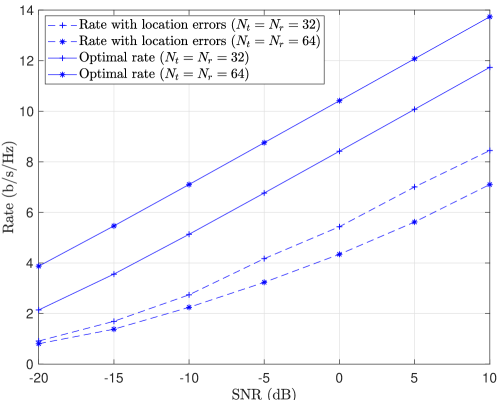
Figure 4: Rate vs SNR for varying number of antennas in the uncertainty region.

As discussed in Section II, we focus on the initial access phase, and the simulations are performed over $10^{3}$ independent blocks. The location estimation and beam alignment are performed at the beginning of each block as summarized in Algorithm I. The metric used to select a beam is the rate loss of the beam compared with the optimal beam pair, where the optimal beams pair are achieved with the precise location information and perfect channel state information. We set the target rate to $95\%$ of the optimal rate, i.e., $R_{0}=0.95\max_{\mathbf{u},\mathbf{v}}R_{d}(\mathbf{u},\mathbf{v})$ except stated otherwise, the size of the window is set to the number of beams that can be processed in each slot (i.e., $W_{\text{BS}}=N_{b}$).

V-B Results and Discussion

Fig. 4 shows the rate as a function of the SNR obtained from the beam vectors corresponding to the initial estimate of $\hat{\phi}_{m}$ and $\hat{\theta}_{m}$ in the uncertainty region. The results are shown with varying number of antennas. A performance loss can be observed when compared with the rates obtained from selecting the optimal beams. From (5) and (6), as the number of antennas increases, the beamwidth becomes narrow, and the severity of beam misalignment increases. As observed from the figure, the use of a low number of array antenna (lower array gain) may outperform a high number of antenna array depending on the severity of the location estimation error. In addition, the result shows that although location information with some degree of precision is expected to be available to 5G systems, beam alignment is required in the uncertainty region of the location information especially for a large number of antenna arrays with narrow beamwidth.

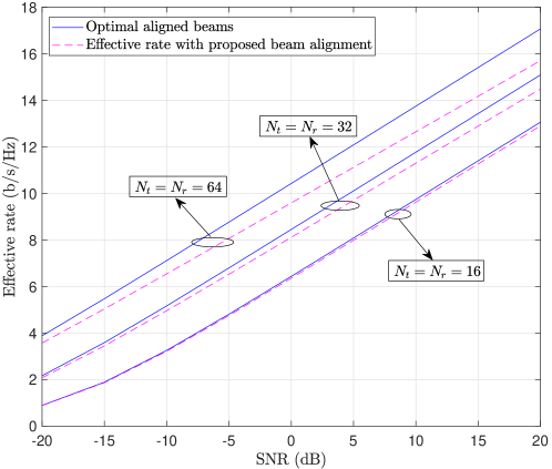
Figure 5: Comparison of rate vs SNR, with varying number of antennas. Fixed parameters: $N_{b}=5,N=100$.

In Fig. 5, we compare the proposed beam alignment scheme with the optimal beam selection scheme. When Fig. 5 is compared with Fig. 4, the effectiveness of the proposed beam alignment can be observed from the rates achieved. When the proposed beam alignment is compared with the optimal aligned beams plots, a performance gap is observed which is due to the beam alignment overhead given by (34). However, to achieve the optimal beam pair, we assume that the channel information of each node is perfectly known which is difficult to achieve in practice. Furthermore, the result shows that exploiting location information can further reduce the beam alignment overhead with a slight penalty on the performance. The beam alignment overhead can be reduced with high precision in the location information. In addition, it can be observed that the gap between the proposed beam alignment scheme and the optimal aligned beam plots increases with an increasing number of antenna which is mainly due to the fact that as the number of antenna increases, the beamwidth decreases. Hence, as the number of beams in the uncertainty region increases, the number of slots $N_{a}$ required for beam alignment also increases.

The proposed algorithm is compared with the results obtained from the Two-Step algorithm in [23], with $N_{t}=N_{r}=64$ antennas in Fig 6. From Fig 6, it can be observed that the proposed scheme outperforms the two step algorithm proposed in [23], even though the penalty of beam alignment is considered in our proposed scheme. This is because in the proposed algorithm, the beam alignment is jointly coordinated by the BS and UE, while in [23], the beam alignment is carried out independently at each node.

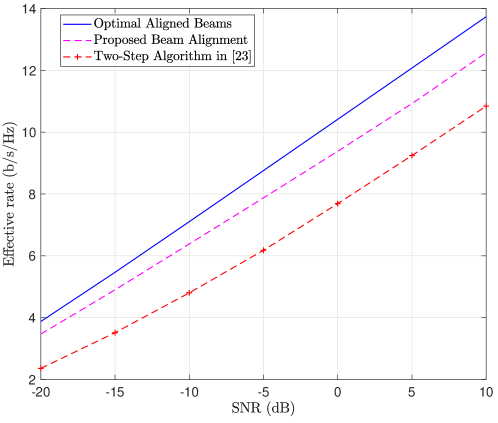
Figure 6: Comparison of proposed scheme and the two step algorithm in [23]. Fixed parameters: $N_{t}=N_{r}=64,N_{b}=5,N=100$.

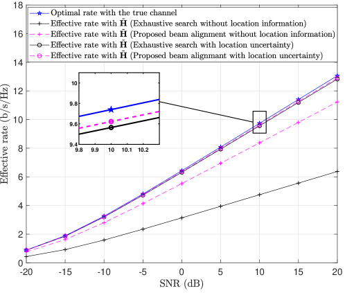
Figure 7: Effective rates with channel estimate as a function of SNR. Fixed parameters: $N_{t}=N_{r}=16,N_{b}=5,N=100$, $R_{0}=\max_{\mathbf{u},\mathbf{v}}R_{d}(\mathbf{u},\>\mathbf{v})$.

Fig. 7 compares the effective rates obtained with the channel estimate as a function of SNR. The plots without location information are obtained by transmitting with the beam set ($\mathcal{V}$ and $\mathcal{U}$). With the knowledge of the location uncertainty region, beam alignment is performed using the beam set ($\mathcal{B}_{\text{BS}}^{m}$ and $\mathcal{B}_{\text{UE}}^{m}$), where $m$ correspond to the LOS path in this plot. In this result, we evaluate the FIM given by (47) and the rates are computed from (60), where the expectation is taken over the channel estimation error matrix. In the plot of the exhaustive search without location information, the channel is estimated by transmitting symbols with each of the 16-dimensional beams vectors in $\mathcal{V}$ and $\mathcal{U}$ since $N_{t}=N_{r}=16$. A performance gap can be observed when the proposed beam alignment is compared with the exhaustive search without location information. The improvement in the proposed algorithm is due to the fast beam alignment procedure discussed in Section III-B3, leading to a small beam alignment penalty when compared to the exhaustive search. With the location information and maximum location estimation error known a priori, the channel parameters can be estimated by transmitting with the few beams in $\mathcal{B}_{\text{BS}}^{m}$ and $\mathcal{B}_{\text{UE}}^{m}$ which correspond to the set of beams vectors in the uncertainty region of the $m$-th path. We plot the effective rate of the exhaustive search and the proposed beam alignment algorithm in the location uncertainty region. It is observed that for a fixed $N_{b}$ and $N$, the performance of both schemes is quite close to the optimal rate plot. This is because there are few beams in the location uncertainty region and hence, the beam alignment overhead is low.

As the number of beams in the uncertainty region increases due to narrow beams at the BS and UE (increasing $N_{r}$ and $N_{t}$), the effect of the search window can be observed, and the efficiency of the proposed scheme with search window become more noticeable as shown in Fig. 8. In the figure, the effective rate of the proposed scheme is plotted showing the effect of the proposed window for varying number of antennas. As the number of antennas increase from $N_{t}=N_{r}=16$ to $N_{t}=N_{r}=64$, the number of beams in the uncertainty region also increase, thereby requiring more slots for beam alignment. However, with the implementation of the search window, the proposed scheme is able to achieve fast beam alignment compared to the plot of the proposed beam alignment scheme without the implementation of the search window, hence, a better effective rate performance is achieved as shown in the result. The improvement obtained from the use of the search window in the proposed scheme is as a result the reduction in the number of beams to be searched after determining the direction of search in the window.

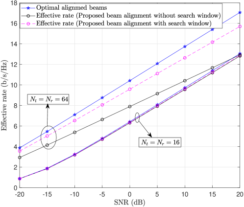
Figure 8: Comparison of the proposed beam alignment scheme with and without search window in the uncertainty region. Fixed parameters: $N_{b}=5$, $N=100$, $R_{0}=\max_{\mathbf{u},\mathbf{v}}R_{d}(\mathbf{u},\>\mathbf{v})$ .

From Fig. 7 and Fig. 8, it can be deduced that with high precision in location information, there is no need to estimate the channel with a large number of beam vectors from $\mathcal{V}$ and $\mathcal{U}$ since similar performance can be achieved with much fewer beam set in the uncertainty region. Intuitively, with some degree of precision of the location information at the BS and UE and the knowledge of the maximum location error, the number of beams required to achieve the best estimate of $\theta$ and $\phi$ can be reduced. Hence, exploiting location information in the proposed scheme reduces the beam alignment overhead.

VI Conclusion

In this paper, we propose a coordinated beam alignment algorithm which exploits the noisy location information of the UE, and potential reflecting points. The proposed beam alignment enables the UE and BS to jointly coordinate the beam alignment to combat the path-loss in the mmWave range. The scheme speeds up the beam alignment procedure by focusing the search in a specific region bounded by the location error margin. Furthermore, an intelligent search is performed in this specific region by searching across a small window of beams to determine the direction of the actual beam. The numerical results show that the proposed algorithm can significantly improve the beam alignment speed when compared to the scenario with perfect channel information and other existing schemes.

Appendix A Proof of Proposition I

Proof:

Without loss of generality, we define $\epsilon_{m}={\gamma}_{m}-{\hat{\phi}}_{m}$ as the half angle of the uncertainty region in path $m$ from the BS as shown in Fig. 2, where ${\gamma}_{m}$ is the angle between the antenna normal and the maximum location error boundary of the node in path $m$. Then we can express

$$y_{m} =\hat{d}_{m}^{\text{BS}}\sin{\hat{\phi}}_{m},$$ (61)

$$x_{m} =\hat{d}_{m}^{\text{BS}}\cos{\hat{\phi}}_{m},$$ (62)

where $\hat{d}_{m}^{\text{BS}}$ can be obtained from equation (17) for the BS, and (18) for the UE. From simple geometry, we can obtain

$$\tan{\gamma}_{m} =\frac{y_{m}+r_{m}^{\text{BS}}}{x_{m}}$$

$$=\frac{\hat{d}_{m}^{\text{BS}}\sin{\hat{\phi}}_{m}+r_{m}^{\text{BS}}}{\hat{d}_{m}^{\text{BS}}\cos{\hat{\phi}}_{m}},\quad m=1,\ldots,M,$$ (63)

by solving for ${\gamma}_{m}$, the following can be obtained

$${\gamma}_{m}=\arctan\left(\frac{\hat{d}_{m}^{\text{BS}}\sin{\hat{\phi}}_{m}+r_{m}^{\text{BS}}}{\hat{d}_{m}^{\text{BS}}\cos{\hat{\phi}}_{m}}\right).$$ (64)

By solving for $\epsilon_{m}={\gamma}_{m}-{\hat{\phi}}_{m}$, equation (64) can be expressed as

$$\epsilon_{m}+{\hat{\phi}}_{m}=\arctan\left(\frac{\hat{d}_{m}^{\text{BS}}\sin{\hat{\phi}}_{m}+r_{m}^{\text{BS}}}{\hat{d}_{m}^{\text{BS}}\cos{\hat{\phi}}_{m}}\right).$$ (65)

Following similar steps from (61) to (65) we obtain

$$\delta_{m}+{\hat{\theta}}_{m}=\arctan\left(\frac{\hat{d}_{m}^{\text{UE}}\sin{\hat{\theta}}_{m}+r_{m}^{\text{UE}}}{\hat{d}_{m}^{\text{UE}}\cos{\hat{\theta}}_{m}}\right),$$ (66)

which concludes the proof.

∎

Appendix B Proof of the entries of the Matrix $\mathbf{J}_{\boldsymbol{\theta}}$

In this section, we present the derivation of the entries of the $\mathbf{J}_{\boldsymbol{\theta}}$.

Proof:

The proof begins with the calculations of

$$\mathbf{J}(\phi_{m},\phi_{m})\triangleq-\mathbb{E}_{\mathbf{y|\boldsymbol{\theta}}}\left[\frac{\partial^{2}L(\mathbf{y})}{\partial\phi_{m}^{2}}\right].$$ (67)

Note that $L(\mathbf{y})$ in (48) is given by the log-likelihood function in (41) and by differentiating $L(\mathbf{y})$ w.r.t $\phi_{m}$, we obtain

$$\frac{\partial L(\mathbf{y})}{\partial\phi_{m}}=\frac{E_{s}}{\sigma^{2}}\left[\left(\mathbf{y}-\mathbf{m}\right)^{\mathsf{H}}\frac{\partial\mathbf{m}}{\partial\phi_{m}}+\frac{\partial\mathbf{m}^{\mathsf{H}}}{\partial\phi_{m}}\left(\mathbf{y}-\mathbf{m}\right)\right],$$ (68)

taking the second differential of (68) w.r.t $\phi_{m}$ we have

$$\frac{\partial^{2}L(\mathbf{y})}{\partial\phi_{m}^{2}} {}={} \frac{E_{s}}{\sigma^{2}}\left[-\frac{\partial\mathbf{m}^{\mathsf{H}}}{\partial\phi_{m}}\frac{\partial\mathbf{m}}{\partial\phi_{m}}+\left(\mathbf{y}-\mathbf{m}\right)^{\mathsf{H}}\frac{\partial^{2}\mathbf{m}}{\partial\phi_{m}^{2}}\right.{+}\left.\frac{\partial^{2}\mathbf{m}^{\mathsf{H}}}{\partial\phi_{m}^{2}}\left(\mathbf{y}-\mathbf{m}\right)-\frac{\partial\mathbf{m}^{\mathsf{H}}}{\partial\phi_{m}}\frac{\partial\mathbf{m}}{\partial\phi_{m}}\right].$$ (69)

By taking the expectation of (69) w.r.t. $L(\mathbf{y})$ we obtain

$$\mathbf{J}(\phi_{m},\phi_{m})=\frac{2E_{s}}{\sigma^{2}}\left[\frac{\partial\mathbf{m}^{\mathsf{H}}}{\partial\phi_{m}}\frac{\partial\mathbf{m}}{\partial\phi_{m}}\right].$$ (70)

Next, we will determine $\partial\mathbf{m}^{\mathsf{H}}/{\partial\phi_{m}}$, where $\mathbf{m}$ is given by (39)

$$\frac{\partial\mathbf{m}^{\mathsf{H}}}{\partial\phi_{m}} {}={} \frac{\partial}{\partial\phi_{m}}\alpha_{m}\biggl{(}\mathbf{a}_{t}^{\mathsf{T}}(\phi_{m})\otimes\mathbf{a}_{r}^{\mathsf{H}}(\theta_{m})\biggr{)}\mathbf{A^{\mathsf{H}}}$$ (71)

$${}={} \alpha_{m}j\pi\sin\phi_{m}\biggl{(}\tilde{\mathbf{a}}_{t}^{\mathsf{H}}(\phi_{m})\otimes\mathbf{a}_{r}^{\mathsf{H}}(\theta_{m})\biggr{)}\mathbf{A^{\mathsf{H}}},$$

where

$$\begin{split}\tilde{\mathbf{a}}_{t}(\phi_{m})=\frac{1}{\sqrt{N_{t}}}\biggl{[}0,\;e^{-j\pi\cos\phi_{m}},\ldots,(N_{t}-1)e^{-j\pi(N_{t}-1)\cos\phi_{m}}\biggr{]}^{\mathsf{T}}.\end{split}$$ (72)

Similarly, $\partial\mathbf{m}/{\partial\phi_{m}}$ can be obtained as

$$\frac{\partial\mathbf{m}}{\partial\phi_{m}}=-\mathbf{A}\alpha_{m}j\pi\sin\phi_{m}\bigg{(}\tilde{\mathbf{a}}_{t}(\phi_{m})\otimes\mathbf{a}_{r}(\theta_{m})\bigg{)}.$$ (73)

By substituting (71) and (73) in (70), we obtain

$$\begin{split}\mathbf{J}(\phi_{m},\phi_{m})=&\frac{2\alpha_{m}^{2}\pi^{2}E_{s}}{\sigma^{2}}\operatorname*{tr}\biggl{(}\mathbf{A^{\mathsf{H}}}\mathbf{A}\big{(}\sin^{2}\phi_{m}\tilde{\mathbf{a}}_{t}(\phi_{m})\tilde{\mathbf{a}}_{t}^{\mathsf{H}}(\phi_{m})\big{)}{\otimes}\big{(}\mathbf{a}_{r}(\theta_{m})\mathbf{a}_{r}^{\mathsf{H}}(\theta_{m})\big{)}\biggr{)},\end{split}$$ (74)

where

$$\begin{split}\tilde{\mathbf{a}}_{r}(\theta_{m})=\frac{1}{\sqrt{N_{r}}}\biggl{[}0,e^{-j\pi\cos\theta_{m}},\ldots,\biggl{.}(N_{r}-1)e^{-j\pi(N_{r}-1)\cos\theta_{m}}\biggr{]}^{\mathsf{T}}.\end{split}$$ (75)

Next, we compute

$$\mathbf{J}(\phi_{m},\theta_{m})\triangleq-\mathbb{E}_{\mathbf{y|\boldsymbol{\theta}}}\left[\frac{\partial^{2}L(\mathbf{y})}{\partial\phi_{m}\partial\theta_{m}}\right],$$ (76)

where we take the second derivative of (68) with respect to $\phi_{m}$ and $\theta_{m}$ given as

$$\frac{\partial^{2}L(\mathbf{y})}{\partial\phi_{m}\partial\theta_{m}}=\frac{E_{s}}{\sigma^{2}}\left[-\frac{\partial\mathbf{m}^{\mathsf{H}}}{\partial\phi_{m}}\frac{\partial\mathbf{m}}{\partial\theta_{m}}+\frac{\partial\mathbf{m}^{\mathsf{H}}}{\partial\theta_{m}}\frac{\partial\mathbf{m}}{\partial\phi_{m}}\right].$$ (77)

The partial derivative of $\mathbf{m}$ w.r.t $\theta_{m}$ can be obtained as

$$\frac{\partial\mathbf{m}}{\partial\theta_{m}}=\alpha_{m}j\pi\sin\theta_{m}\mathbf{A}\big{(}\mathbf{a}_{t}^{*}(\phi_{m})\otimes\tilde{\mathbf{a}}_{r}^{*}(\theta_{m})\big{)},$$ (78)

where the partial derivative of $\mathbf{m}^{\mathsf{H}}$ w.r.t $\theta_{m}$ can be obtained similarly as

$$\frac{\partial\mathbf{m}^{\mathsf{H}}}{\partial\theta_{m}}=-\alpha_{m}j\pi\sin\theta_{m}\big{(}\mathbf{a}_{t}^{\mathsf{T}}(\phi_{m})\otimes\tilde{\mathbf{a}}_{r}^{\mathsf{T}}(\theta_{m})\big{)}\mathbf{A}^{\mathsf{H}}.$$ (79)

By substituting (71), (73), (78) and (79) into (77), and using the properties in Lemma 1, (76) can be simplified as

$$\mathbf{J}\left(\phi_{m},\theta_{m}\right)=\frac{-2\alpha_{m}^{2}\pi^{2}E_{s}}{\sigma^{2}}\operatorname{Re}\biggl{\{}\operatorname*{tr}\biggl{(}\mathbf{A^{\mathsf{H}}}\mathbf{A}\big{(}\sin\phi_{m}\tilde{\mathbf{a}}_{t}(\phi_{m})\mathbf{a}_{r}^{\mathsf{T}}(\theta_{m})\big{)}{\otimes}\big{(}\sin\theta_{m}\mathbf{a}_{t}(\phi_{m})\tilde{\mathbf{a}}_{r}^{\mathsf{T}}(\theta_{m})\big{)}\biggr{)}\biggr{\}},$$ (80)

where Re$\left\{x\right\}$ denotes the real part of the complex variable $x$.

Next, we compute

$$\mathbf{J}(\phi_{m},\alpha_{m})\triangleq-\mathbb{E}_{\mathbf{y|\boldsymbol{\theta}}}\left[\frac{\partial^{2}L(\mathbf{y})}{\partial\phi_{m}\partial\alpha_{m}}\right],$$ (81)

which can be obtained by taking the second derivative of (68) with respect to $\phi_{m}$ and $\alpha_{m}$ given as,

$$\frac{\partial^{2}L(\mathbf{y})}{\partial\phi_{m}\partial\alpha_{m}}=\frac{E_{s}}{\sigma^{2}}\left[\frac{\partial\mathbf{m}^{\mathsf{H}}}{\partial\phi_{m}}\frac{\partial\mathbf{m}}{\partial\alpha_{m}}+\frac{\partial\mathbf{m}^{\mathsf{H}}}{\partial\alpha_{m}}\frac{\partial\mathbf{m}}{\partial\phi_{m}}\right],$$ (82)

where

$$\frac{\partial\mathbf{m}}{\partial\alpha_{m}}=\mathbf{A}\big{(}\mathbf{a}_{t}^{*}(\phi_{m})\otimes\mathbf{a}_{r}(\theta_{m})\big{)},$$ (83)

and

$$\frac{\partial\mathbf{m}^{\mathsf{H}}}{\partial\alpha_{m}}=\big{(}\mathbf{a}_{t}^{\mathsf{T}}(\phi_{m})\otimes\mathbf{a}_{r}^{\mathsf{H}}(\theta_{m})\big{)}\mathbf{A}^{\mathsf{H}}.$$ (84)

By using the properties defined in Lemma 1 and substituting (71), (73), (83) and (84) into (82) we obtain

$$\mathbf{J}(\phi_{m},\alpha_{m})=\frac{-2\alpha_{m}\pi E_{s}}{\sigma^{2}}\operatorname{Im}\biggl{\{}\operatorname*{tr}\biggl{(}\mathbf{A}^{\mathsf{H}}\mathbf{A}\big{(}\sin\phi_{m}\mathbf{a}_{t}^{*}(\phi_{m})\tilde{\mathbf{a}}_{t}^{\mathsf{H}}(\phi_{m})\big{)}\otimes\left(\mathbf{a}_{r}(\theta_{m})\mathbf{a}_{r}^{\mathsf{H}}(\theta_{m})\right)\biggr{)}\biggr{\}},$$ (85)

where Im$\left\{x\right\}$ is the imaginary part of the complex variable $x$.

Next, we determine $\mathbf{J}(\theta_{m},\theta_{m})$ from

$$\mathbf{J}(\theta_{m},\theta_{m})\triangleq-\mathbb{E}_{\mathbf{y|\boldsymbol{\theta}}}\left[\frac{\partial^{2}L(\mathbf{y})}{\partial\theta_{m}^{2}}\right],$$ (86)

similar to (70) as follows

$$\mathbf{J}(\theta_{m},\theta_{m})=\frac{2E_{s}}{\sigma^{2}}\left[\frac{\partial\mathbf{m}^{\mathsf{H}}}{\partial\theta_{m}}\frac{\partial\mathbf{m}}{\partial\theta_{m}}\right],$$ (87)

which can be evaluated by substituting (78) and (79) into (87) as

$$\mathbf{J}(\theta_{m},\theta_{m}) {}={} \frac{2\alpha_{m}^{2}\pi^{2}E_{s}\sin^{2}\theta_{m}}{\sigma^{2}}\biggl{[}\big{(}\mathbf{a}_{t}^{\mathsf{T}}(\phi_{m})\otimes\tilde{\mathbf{a}}_{r}^{\mathsf{T}}(\theta_{m})\big{)}\times\mathbf{A}^{\mathsf{H}}\mathbf{A}\left(\mathbf{a}_{t}^{*}(\phi_{m})\otimes\tilde{\mathbf{a}}_{r}^{*}(\theta_{m})\right)\biggr{]}$$ (88)

$${}={} \frac{2\alpha_{m}^{2}\pi^{2}E_{s}}{\sigma^{2}}\operatorname*{tr}\biggl{(}\mathbf{A}^{\mathsf{H}}\mathbf{A}\big{(}\mathbf{a}_{t}^{*}(\phi_{m})\mathbf{a}_{t}^{\mathsf{T}}(\phi_{m})\big{)}\otimes\big{(}\tilde{\mathbf{a}}_{r}(\theta_{m})\tilde{\mathbf{a}}_{r}^{\mathsf{H}}(\theta_{m})\sin^{2}\theta_{m}\big{)}\biggr{)}.$$

Next, we evaluate the entries of $\mathbf{J}(\theta_{m},\alpha_{m})$ defined as

$$\mathbf{J}(\theta_{m},\alpha_{m})\triangleq-\mathbb{E}_{\mathbf{y|\boldsymbol{\theta}}}\left[\frac{\partial^{2}L(\mathbf{y})}{\partial\theta_{m}\partial\alpha_{m}}\right],$$ (89)

where the second derivative of (68) is taken with respect to respect to $\theta_{m}$ and $\alpha_{m}$ as follows

$$\mathbf{J}(\theta_{m},\alpha_{m})=\frac{E_{s}}{\sigma^{2}}\left[\frac{\partial\mathbf{m}^{\mathsf{H}}}{\partial\theta_{m}}\frac{\partial\mathbf{m}}{\partial\alpha_{m}}+\frac{\partial\mathbf{m}^{\mathsf{H}}}{\partial\alpha_{m}}\frac{\partial\mathbf{m}}{\partial\theta_{m}}\right],$$ (90)

which can be evaluated by substituting (78), (79), (83) and (84) into (90) as follows

$$\mathbf{J}(\theta_{m},\alpha_{m}) {}={} \frac{2\alpha_{m}\pi E_{s}}{\sigma^{2}}\sin\theta_{m}\operatorname{Im}\biggl{\{}\big{(}\mathbf{a}_{t}^{\mathsf{T}}(\phi_{m})\otimes\tilde{\mathbf{a}}_{r}^{\mathsf{T}}(\theta_{m})\big{)}\times\mathbf{A}^{\mathsf{H}}\mathbf{A}\big{(}\mathbf{a}_{t}^{*}(\phi_{m})\otimes\mathbf{a}_{r}(\theta_{m})\big{)}\biggr{\}}$$ (91)

$${}={} \frac{2\alpha_{m}j\pi E_{s}}{\sigma^{2}}\operatorname{Im}\biggl{\{}\operatorname*{tr}\biggl{(}\mathbf{A}^{\mathsf{H}}\mathbf{A}\big{(}\mathbf{a}_{t}^{*}(\phi_{m})\mathbf{a}_{t}^{\mathsf{T}}(\phi_{m})\big{)}\otimes\big{(}\sin\theta_{m}\mathbf{a}_{r}(\theta_{m})\tilde{\mathbf{a}}_{r}^{\mathsf{T}}(\theta_{m})\big{)}\biggr{)}\biggr{\}}.$$

Finally, the factor

$$\mathbf{J}(\alpha_{m},\alpha_{m})\triangleq-\mathbb{E}_{\mathbf{y|\boldsymbol{\theta}}}\left[\frac{\partial^{2}L(\mathbf{y})}{\partial\alpha_{m}^{2}}\right]$$ (92)

can be evaluated as:

$$\mathbf{J}(\alpha_{m},\alpha_{m})=\frac{2E_{s}}{\sigma^{2}}\left[\frac{\partial\mathbf{m}^{\mathsf{H}}}{\partial\alpha_{m}}\frac{\partial\mathbf{m}}{\partial\alpha_{m}}\right],$$ (93)

where the parameters $\partial\mathbf{m}^{\mathsf{H}}/{\partial\alpha_{m}}$ and ${\partial\mathbf{m}}/{\partial\alpha_{m}}$ can be obtained by substituting (83) and (84) into (93), from which we obtain

$$\mathbf{J}(\alpha_{m},\alpha_{m}) =\frac{2E_{s}}{\sigma^{2}}\operatorname*{tr}\biggl{(}\big{(}\mathbf{a}_{t}^{\mathsf{T}}(\phi_{m})\otimes\mathbf{a}_{r}^{\mathsf{H}}(\theta_{m})\mathbf{A}^{\mathsf{H}}\mathbf{A}\big{(}\mathbf{a}_{t}^{*}(\phi_{m})\otimes\mathbf{a}_{r}(\theta_{m})\big{)}\biggr{)}$$

$$=\frac{2E_{s}}{\sigma^{2}}\operatorname*{tr}\biggl{(}\mathbf{A}^{\mathsf{H}}\mathbf{A}\big{(}\mathbf{a}_{t}^{*}(\phi_{m})\otimes\mathbf{a}_{r}(\theta_{m})\big{)}\big{(}\mathbf{a}_{t}^{\mathsf{T}}(\phi_{m})\otimes\mathbf{a}_{r}^{\mathsf{H}}(\theta_{m})\big{)}\biggr{)}$$

$$=\frac{2E_{s}}{\sigma^{2}}\operatorname*{tr}\biggl{(}\mathbf{A}^{\mathsf{H}}\mathbf{A}\big{(}\mathbf{a}_{t}^{*}(\phi_{m})\mathbf{a}_{t}^{\mathsf{T}}(\phi_{m})\big{)}{\otimes}\big{(}\mathbf{a}_{r}(\theta_{m})\mathbf{a}_{r}^{\mathsf{H}}(\theta_{m})\big{)}\biggr{)}.$$ (94)

This concludes the proof of the entries of $\mathbf{J}_{\boldsymbol{\theta}}$. ∎

References

• [1] I. Orikumhi, J. Kang, C. Park, J. Yang, and S. Kim, “Location-aware coordinated beam alignment in mmwave communication,” in 2018 56th Annual Allerton Conference on Communication, Control, and Computing (Allerton), Oct. 2018, pp. 386–390.
• [2] T. S. Rappaport, S. Sun, R. Mayzus, H. Zhao, Y. Azar, K. Wang, G. N. Wong, J. K. Schulz, M. Samimi, and F. Gutierrez, “Millimeter wave mobile communications for 5G cellular: It will work!” IEEE Access, vol. 1, pp. 335–349, 2013.
• [3] M. Hussain and N. Michelusi, “Energy efficient beam-alignment in millimeter wave networks,” in 2017 51st Asilomar Conference on Signals, Systems, and Computers, Oct. 2017, pp. 1219–1223.
• [4] I. Mavromatis, A. Tassi, R. J. Piechocki, and A. Nix, “Beam alignment for millimetre wave links with motion prediction of autonomous vehicles,” in Antennas, Propagation RF Technology for Transport and Autonomous Platforms 2017, Feb. 2017, pp. 1–8.
• [5] X. Song, S. Haghighatshoar, and G. Caire, “A robust time-domain beam alignment scheme for multi-user wideband mmWave systems,” in WSA 2018; 22nd International ITG Workshop on Smart Antennas, Mar. 2018, pp. 1–7.
• [6] V. Va, J. Choi, and R. W. Heath, “The impact of beamwidth on temporal channel variation in vehicular channels and its implications,” IEEE Trans. Veh. Technol., vol. 66, no. 6, pp. 5014–5029, Jun. 2017.
• [7] M. Cheng, J. B. Wang, Y. Wu, X. G. Xia, K. K. Wong, and M. Lin, “Coverage analysis for millimeter wave cellular networks with imperfect beam alignment,” IEEE Trans. Veh. Technol., pp. 1–1, 2018.
• [8] C. Liu, M. Li, S. V. Hanly, I. B. Collings, and P. Whiting, “Millimeter wave beam alignment: Large deviations analysis and design insights,” IEEE J. Sel. Areas Commun., vol. 35, no. 7, pp. 1619–1631, Jul. 2017.
• [9] S. Noh, M. D. Zoltowski, and D. J. Love, “Multi-resolution codebook and adaptive beamforming sequence design for millimeter wave beam alignment,” IEEE Trans. Wireless Commun., vol. 16, no. 9, pp. 5689–5701, Sep. 2017.
• [10] M. Giordani, M. Polese, A. Roy, D. Castor, and M. Zorzi, “A tutorial on beam management for 3GPP NR at mmWave frequencies,” arXiv preprint arXiv:1804.01908, 2018.
• [11] ——, “Initial access frameworks for 3GPP NR at mmWave frequencies,” in 2018 17th Annual Mediterranean Ad Hoc Networking Workshop (Med-Hoc-Net), Jun. 2018, pp. 1–8.
• [12] C. N. Barati, S. A. Hosseini, S. Rangan, P. Liu, T. Korakis, and S. S. Panwar, “Directional cell search for millimeter wave cellular systems,” in 2014 IEEE 15th International Workshop on Signal Processing Advances in Wireless Communications (SPAWC), Jun. 2014, pp. 120–124.
• [13] C. Liu, M. Li, I. B. Collings, S. V. Hanly, and P. Whiting, “Design and analysis of transmit beamforming for millimeter wave base station discovery,” IEEE Trans. Wireless Commun., vol. 16, no. 2, pp. 797–811, Feb. 2017.
• [14] Y. Li, J. Luo, M. H. Castaneda, N. Vucic, W. Xu, and G. Caire, “Analysis of broadcast signaling for millimeter wave cell discovery,” in 2017 IEEE 86th Vehicular Technology Conference (VTC-Fall), Sep. 2017, pp. 1–5.
• [15] S. Habib, S. A. Hassan, A. A. Nasir, and H. Mehrpouyan, “Millimeter wave cell search for initial access: Analysis, design, and implementation,” in 2017 13th International Wireless Communications and Mobile Computing Conference (IWCMC), Jun. 2017, pp. 922–927.
• [16] C. N. Barati, S. A. Hosseini, M. Mezzavilla, T. Korakis, S. S. Panwar, S. Rangan, and M. Zorzi, “Initial access in millimeter wave cellular systems,” IEEE Trans. Wireless Commun., vol. 15, no. 12, pp. 7926–7940, Dec. 2016.
• [17] Y. Li, J. G. Andrews, F. Baccelli, T. D. Novlan, and J. Zhang, “On the initial access design in millimeter wave cellular networks,” in 2016 IEEE Globecom Workshops (GC Wkshps), Dec. 2016, pp. 1–6.
• [18] S. Hur, T. Kim, D. J. Love, J. V. Krogmeier, T. A. Thomas, and A. Ghosh, “Millimeter wave beamforming for wireless backhaul and access in small cell networks,” IEEE Trans. Commun., vol. 61, no. 10, pp. 4391–4403, Oct. 2013.
• [19] W. C. Chen, H. T. Chiu, and R. H. Gau, “Bayesian tree search for beamforming training in millimeter wave wireless communication systems,” in 2018 IEEE Wireless Communications and Networking Conference (WCNC), Apr. 2018, pp. 1–6.
• [20] R. D. Taranto, S. Muppirisetty, R. Raulefs, D. Slock, T. Svensson, and H. Wymeersch, “Location-aware communications for 5G networks: How location information can improve scalability, latency, and robustness of 5G,” IEEE Signal Process. Mag., vol. 31, no. 6, pp. 102–112, Nov. 2014.
• [21] H. Wymeersch, N. Garcia, H. Kim, G. Seco-Granados, S. Kim, F. Went, and M. Fröhle, “5G mmWave downlink vehicular positioning,” in 2018 IEEE Global Communications Conference (GLOBECOM).   IEEE, 2018, pp. 206–212.
• [22] G. C. Alexandropoulos, “Position aided beam alignment for millimeter wave backhaul systems with large phased arrays,” in 2017 IEEE 7th International Workshop on Computational Advances in Multi-Sensor Adaptive Processing (CAMSAP), Dec. 2017, pp. 1–5.
• [23] F. Maschietti, D. Gesbert, P. de Kerret, and H. Wymeersch, “Robust location-aided beam alignment in millimeter wave massive MIMO,” arXiv preprint arXiv:1705.01002, 2017.
• [24] A. Shahmansoori, G. E. Garcia, G. Destino, G. Seco-Granados, and H. Wymeersch, “Position and orientation estimation through millimeter-wave MIMO in 5G systems,” IEEE Trans. Wireless Commun., vol. 17, no. 3, pp. 1822–1835, Mar. 2018.
• [25] A. Alkhateeb, Y. H. Nam, M. S. Rahman, J. Zhang, and R. W. Heath, “Initial beam association in millimeter wave cellular systems: Analysis and design insights,” IEEE Trans. Wireless Commun., vol. 16, no. 5, pp. 2807–2821, May 2017.
• [26] A. Alkhateeb, O. E. Ayach, G. Leus, and R. W. Heath, “Channel estimation and hybrid precoding for millimeter wave cellular systems,” IEEE J. Sel. Topics Signal Process., vol. 8, no. 5, pp. 831–846, Oct. 2014.
• [27] J. Zhang, Y. Huang, Q. Shi, J. Wang, and L. Yang, “Codebook design for beam alignment in millimeter wave communication systems,” IEEE Trans. Commun., vol. 65, no. 11, pp. 4980–4995, Nov. 2017.
• [28] N. Garcia, H. Wymeersch, E. G. Ström, and D. Slock, “Location-aided mm-wave channel estimation for vehicular communication,” in 2016 IEEE 17th International Workshop on Signal Processing Advances in Wireless Communications (SPAWC), Jul. 2016, pp. 1–5.
• [29] Study on Downlink Multiuser Superposition Transmission for LTE.   3rd Generation Partnership Project, 3GPP, Document RP250456, Mar. 2015.
• [30] P. Stoica and A. Nehorai, “Music, maximum likelihood, and cramer-rao bound,” IEEE Transactions on Acoustics, Speech, and Signal Processing, vol. 37, no. 5, pp. 720–741, 1989.
• [31] H. V. Poor, An introduction to signal detection and estimation.   Springer Science & Business Media, 2013.
• [32] S. M. Kay, Fundamentals of statistical signal processing : estimation theory.   Englewood Cliffs, N.J : PTR Prentice-Hall, 1993.
• [33] J. Brewer, “Kronecker products and matrix calculus in system theory,” IEEE Trans. Circuits Syst., vol. 25, no. 9, pp. 772–781, 1978.
• [34] A. Graham, Kronecker products and matrix calculus with applications.   Courier Dover Publications, 2018.