A Mean Field Games approach
to Cluster Analysis

In this paper, we develop a Mean Field Games approach to Cluster Analysis. We consider a finite mixture model, given by a convex combination of probability density functions, to describe the given data set. We interpret a data point as an agent of one of the populations represented by the components of the mixture model, and we introduce a corresponding optimal control problem. In this way, we obtain a multi-population Mean Field Games system which characterizes the parameters of the finite mixture model. Our method can be interpreted as a continuous version of the classical Expectation-Maximization algorithm.

AMS-Subject Classification: 62H30, 35J47, 49N70, 91C20.
Keywords: mixture model; Cluster Analysis; Expectation-Maximization algorithm; Mean Field Games; multi-population model.

1 Introduction

Cluster Analysis, a classical problem in unsupervised Machine Learning, concerns the repartition of a group of data points into subgroups, in such a way that the elements within a same group are more similar to each other than they are to the elements of a different one. Clustering methods can be used either to infer specific patterns in rough data sets, or as a preliminary analysis in supervised Machine Learning algorithms (for a review of the applications of cluster analysis, see [6, 23]). Algorithms for Cluster Analysis are generically divided into two classes: hard clustering methods, whose prototype is the K-means algorithm and its variants, for which each data point belongs only to a single subgroup [8]; soft clustering methods, such as the Expectation-Maximization and the Fuzzy K-means algorithms, for which each data point has a certain degree or probability to belong to each cluster [7, 21].

Most of the mathematical literature on Cluster Analysis, and more in general on Machine Learning, is in the framework of finite-dimensional optimization. But recently, different approaches based on partial differential equations and infinite dimensional optimization have begun to be pursued [11, 12, 15]. Even if, in most of the cases, it is not clear if these new approaches are computationally competitive with the traditional ones, they offer new points of view and insights in this rapidly developing field.

In this paper, we propose an approach to Cluster Analysis based on Mean Field Games (MFG in short). This theory was introduced by Lasry and Lions [19] in the framework of differential games with a large number of rational agents. Although it was realized from the beginning that, in perspective, one of the most promising application of MFG theory could be the “Big Data” analysis [18], up to now most of the applications are in the fields of Economics and Financial Mathematics, and only very few papers deal with data analysis problems [22, 5]. Nevertheless, a MFG version of the classical hard-clustering K-means algorithm has been recently proposed in [14]. Relying on a similar approach, here we deal with a MFG version of the soft clustering Expectation-Maximization algorithm.

As in the classical Expectation-Maximization (EM in short) algorithm, the starting point of our analysis is a finite mixture model given by convex combinations of probability density functions (PDFs in short)

$$m(x)=\sum_{k=1}^{K}\alpha_{k}m_{k}(x),\ x\in\mathbb{R}^{d},\quad\text{with}\quad\sum_{k=1}^{K}\alpha_{k}=1.$$

Finite mixture models are powerful probabilistic techniques to describe complex scenarios, e.g. several regions with high mass density, and populations composed by different sub-populations, each one represented by a PDF. Generally, the components of the mixture are assumed to be parametrized PDFs. For example, for a Gaussian mixture model, the parameters are represented by the mean and the variance of each component. Then, the EM algorithm is a technique which allows to compute the unknown coefficients (weights and parameters) of the mixture by incrementally increasing the maximum likelihood with respect to the data set.

In our approach, we are given a PDF $f$ on $\mathbb{R}^{d}$ representing the data set, and we aim to find a corresponding mixture model in order to subdivide the points in $K$ clusters. We interpret the data points as agents belonging with a certain probability to one of the $K$ sub-populations, which are described by a PDF $m_{k}$ with appropriate weights $\alpha_{k}$ on the entire population. The similarity, or proximity, among the members of a same sub-population is encoded in the cost functions of the optimal control problems for each sub-population, which push the agents to aggregate around the closer barycentre of the distributions $m_{k}$.

In order to characterize the components of the mixture model, i.e. the PDFs $m_{k}$ and the weights $\alpha_{k}$, we first consider the case of a quadratic MFG system

$$\left\{\begin{array}[]{ll}-\varepsilon\Delta u_{k}(x)+\frac{1}{2}|Du_{k}(x)|^{2}+\lambda_{k}=\frac{1}{2}(x-\mu_{k})^{t}(\Sigma_{k}^{-1})^{t}\Sigma_{k}^{-1}(x-\mu_{k}),&x\in\mathbb{R}^{d},\\[8.0pt] \varepsilon\Delta m_{k}(x)+{\rm div}(m_{k}(x)Du_{k}(x))=0,&x\in\mathbb{R}^{d},\\[8.0pt] \alpha_{k}=\int_{\mathbb{R}^{d}}\gamma_{k}(x)f(x)dx,\\[8.0pt] m_{k}\geq 0,\,\int_{\mathbb{R}^{d}}m_{k}(x)dx=1,u_{k}(\mu_{k})=0,\end{array}\right.$$ (1.1)

for $k=1,\dots,K$, where the coupling among the different populations is encoded in the right hand side of the first equation. Indeed, the mean $\mu_{k}$ and the covariance matrix $\Sigma_{k}$ of the population $m_{k}$ depend, besides data set $f$, on the whole measure $m$ through the quantities $\gamma_{k}(x)=\alpha_{k}m_{k}(x)/m(x)$. The latter play a central role in the model because they represent the degree of membership of agents to a given population $k$. We introduce a notion of consistency with the data set, and we show that a solution of the multi-population MFG system (1.1) is given by a consistent Gaussian mixture with the same mean and variance of $f$. Moreover, any consistent Gaussian mixture can be obtained as a solution of the MFG system. We remark that the main difference between our approach and the classical EM algorithm, which is an iterative procedure, is that the MFG method gives the partition into clusters as the result of the solution of a stationary system of PDEs.

Then we consider a stationary multi-population MFG system, where the Hamiltonian and the coupling terms can be very general, and we show that it always admits a solution. Note that, in this framework, it is not reasonable to obtain uniqueness, since there may be several admissible partitions of a given data set. We also consider a two-step numerical approximation of the MFG system, inspired to the classical EM algorithm, and we test the method on discrete and continuous data sets.

The paper is organized as follows. In Section 2, following [6, 7], we briefly introduce the K-means and the Expectation Maximization algorithms, in their classical approach. In Section 3, we first describe the approach in [14] and then we propose a quadratic multi-population MFG model for Gaussian finite mixture models. In Section 4, we study a general class of MFG systems for Cluster Analysis. Finally, in Section 5, we perform some numerical tests to confirm the theoretical results.

2 Clustering Algorithms

In this section, we briefly review some classical algorithms for Cluster Analysis. We start by describing the K-means algorithm, a hard clustering technique, hence the Expectation-Maximization algorithm, a soft clustering one. For a complete introduction to the subject, we refer to [6, Cap. 9].
In the following, we are given a set of observable data $\mathcal{X}=\{x_{1},\dots,x_{I}\}$ in $\mathbb{R}^{d}$ and a fixed number $K$ of clusters $S_{j},\ j=1,\dots,K$, into which we want to partition our observations.

2.1 K-Means algorithm

The K-means algorithm is an iterative procedure that assigns points to the nearest cluster with respect to the Euclidean distance, even though other distances can be considered. We denote by $\mu=\{\mu_{1},\mu_{2},\dots,\mu_{K}\}$, $\mu_{k}\in\mathbb{R}^{d}$, the vector of barycentres of the clusters $\{S_{1},S_{2},...,S_{K}\}$. Moreover, we introduce a vector of cluster assignment, $c=(c_{1},c_{2},\dots,c_{I})$, $c_{i}\in\{1,\dots K\}$, such that for every vector $x_{i}\in\mathcal{X}$, we have $c_{i}=k\Leftrightarrow x_{i}\in S_{k}.$
The goal is to find the vectors $\mu$ and $c$ in order to minimize the functional

$$J=\sum_{i=1}^{I}\sum_{k=1}^{K}{\mathbbm{1}_{\{c_{i}=k\}}}|x_{i}-\mu_{k}|^{2}\,,$$ (2.1)

representing the sum of the distances of the data points to the corresponding barycentres ($\mathbbm{1}$ denotes the characteristic function). Starting from an arbitrary assignment for the vector $\mu^{0}$, the $n^{th}$ iteration of the K-means algorithm alternates two steps:

• Cluster assignment: Minimization of the objective function $J$ with respect to $c$ by assigning the point $x_{i}$ to the closest barycentre, i.e.

  $$c^{n}_{i}={\arg\min}_{j}|x_{i}-\mu^{n}_{j}|^{2}\qquad\forall i=1,\dots,I.$$

• Barycentre update: Computation of the new barycentres $\mu^{n+1}_{k}$ of the cluster $S^{n}_{k}=\{x_{i}\in\mathcal{X}:\,c^{n}_{i}=k\}$, i.e.

  $$\mu^{n+1}_{k}=\dfrac{\sum_{i=1}^{I}x_{i}\mathbbm{1}_{\{c^{n}_{i}=k\}}}{\sum_{i=1}^{I}\mathbbm{1}_{\{c^{n}_{i}=k\}}}=\dfrac{\sum_{i=1}^{I}x_{i}\mathbbm{1}_{\{c^{n}_{i}=k\}}}{\text{card}(S^{n}_{k})}\qquad\forall k=1,\dots,K.$$

At each iteration, the objective function $J$ decreases and the algorithm is repeated until there is no change in the cluster assignments, up to a tolerance error.

2.2 Finite mixture model and EM algorithm

Mixture models are probabilistic techniques used to represent complex scenarios of data, and they are related to soft clustering methods which consider a probabilistic partition of the data points into clusters, whose corresponding parametrized probabilities are computed via the EM algorithm. In this setting, we assume that the data set $\mathcal{X}$ represents a set of (independent and identically distributed) observations of a random variable $X$, with unknown distribution that we aim to approximate with a distribution $P$. Moreover, we assume that $P$ is given by a mixture of probability densities $p_{k}(x|\theta_{k})$, depending on some parameters $\theta_{k}$, with mixing coefficients $\alpha_{k}$ such that $\sum_{k=1}^{K}\alpha_{k}=1$, i.e.

$$P(x)=\sum_{k=1}^{K}\alpha_{k}p_{k}(x|\theta_{k}).$$ (2.2)

The purpose is to compute the parameters $\alpha=(\alpha_{1},\dots,\alpha_{k})$, $\theta=(\theta_{1},\dots,\theta_{k})$ of the mixture model (2.2) in order to maximize the likelihood objective function

$$\ln P(\mathcal{X}|\alpha,\theta)=\sum_{i=1}^{I}\left(\ln\sum_{k=1}^{K}\alpha_{k}p_{k}(x_{i}|\theta_{k})\right)$$

with respect to data set $\mathcal{X}$. To simplify the computation of the extrema of the previous functional, the data set $\mathcal{X}$ is considered as incomplete, and it is introduced a random variable $\mathcal{Y}=\{y_{i}\}_{i=1}^{I}$ whose values $y_{i}$ specify the component of $P$ generating the point, i.e. $y_{i}\in\{1,\dots,K\}$ and $y_{i}=k$ if and only if the point $x_{i}$ has been generated by the distribution $p_{k}$. We define the responsibility of $x_{i}$ with respect to the k-th cluster as

$$\gamma_{k}(x_{i}):=p_{k}(y_{i}=k|x_{i},\theta_{k}),$$ (2.3)

i.e. as the probability of an assignment $y_{i}$ once we have observed $x_{i}$; the EM algorithm aims to find a maximum of the expected value of the complete data log-likelihood functional

$$\mathbb{E}_{\mathcal{Y}}[\ln p(\mathcal{X,Y}|\theta_{k},\alpha_{k})]=\sum_{i=1}^{I}\sum_{k=1}^{K}\gamma_{k}(x_{i})\ln(\alpha_{k}p_{k}(x_{i}|\theta_{k}))$$ (2.4)

(see formula (9.40) in [6]). It takes a particular simple and explicit form if we consider parametric distributions $p_{k}(x|\theta_{k})$ given by Gaussian distributions ${\cal N}(x|\mu_{k},\Sigma_{k})$. Starting from an arbitrary initialization $\mu^{0}_{k}$, $\Sigma^{0}_{k}$, $\alpha_{k}^{0}$, $k=1,\dots,K$, and computing the optimality conditions for the functional (2.4) with respect to $\gamma_{k}$ for $\alpha_{k},\mu_{k},\Sigma_{k}$ fixed, and then exchanging the roles, we get the following two alternating steps:

• E-step: Given $\mu^{n-1}_{k}$ $\Sigma^{n-1}_{k}$, $\alpha^{n-1}_{k}$, $k=1,\dots,K$, compute the posterior probability (responsibility) of a datum $x_{i}$ to belong to the cluster $S_{k}$

  $$\gamma^{n}_{k}(x_{i})=P(y_{i}=k|x_{i},\mu^{n-1}_{k},\Sigma^{n-1}_{k})=\dfrac{\alpha^{n-1}_{k}\mathcal{N}(x_{i}|\mu^{n-1}_{k},\Sigma^{n-1}_{k})}{\sum_{j=1}^{K}\alpha^{n-1}_{j}\mathcal{N}(x_{i}|\mu^{n-1}_{j},\Sigma^{n-1}_{j})}.$$

• M-step: Update the parameters $\alpha$, $\mu$, $\Sigma$, by setting for $k=1,\dots,K$,

  $$\alpha^{n}_{k}=\dfrac{\sum_{i=1}^{I}\gamma^{n}_{k}(x_{i})}{I},$$

  $$\mu^{n}_{k}=\dfrac{\sum_{i=1}^{N}x_{i}\gamma^{n}_{k}(x_{i})}{\sum_{i=1}^{I}\gamma^{n}_{k}(x_{i})},$$ (2.5)

  $$\Sigma^{n}_{k}=\dfrac{\sum_{i=1}^{N}\gamma^{n}_{k}(x_{i})(x_{i}-\mu^{n}_{k})(x_{i}-\mu^{n}_{k})^{t}}{\sum_{i=1}^{I}\gamma^{n}_{k}(x_{i})}.$$ (2.6)

After the convergence of the algorithm under some appropriate stopping criterion, we interpret the responsibility $\gamma_{k}(x_{i})$ as the probability that $x_{i}$ belongs to the cluster $S_{k}$.

It is interesting to observe that the K-means algorithm can be derived as a limit of the EM algorithm when the variances of the mixture model (2.4) go to zero. Indeed, assume for simplicity that the covariance matrix is $\Sigma_{k}=\sigma I$, $k=1,\dots,K$ , where $I$ is the identity $d\times d$ matrix and $\sigma>0$ a constant. In this case, the responsibilities in (2.3) are given by

$$\gamma_{k}(x_{i})=\dfrac{\alpha_{k}e^{-\frac{|x_{i}-\mu_{k}|^{2}}{2\sigma}}}{\sum_{j=1}^{K}\alpha_{j}e^{-\frac{|x_{i}-\mu_{j}|^{2}}{2\sigma}}}.$$

For $\sigma\rightarrow 0$, the responsibility $\gamma_{k}(x_{i})$, corresponding to index $k$ minimizing the distance of the barycentre $\mu_{k}$ from $x_{i}$, tends to $1$, while, for $j\neq k$, all the other responsibilities $\gamma_{j}(x_{i})$ go to $0$. Hence, at least formally, $\gamma_{k}(x_{i})\rightarrow\mathbbm{1}_{\{c_{i}=k\}}$ and the maximum likelihood functional (2.4) tends, up to a constant, to the K-means functional $J$ defined in (2.1) (see [6, Sec. 9.3.2]).

3 MFG models for Cluster Analysis

In this section, we describe some models for Cluster Analysis based on MFG theory. In the classical MFG theory (see [19]), we have a continuum of indistinguishable agents whose dynamics, driven by independent Brownian motions $W_{t}$, is given by

$$\begin{cases}dX_{t}=a_{t}dt+\sqrt{2\epsilon}dW_{t},\qquad t>0\\ X_{0}=x.\end{cases}$$ (3.1)

The function $a_{t}$ represents the control which an agent chooses in order to minimize a cost function $J$, to be specified according to the considered model. Most of the time, the cost $J$ comprises a term $L(x,a)$ depending on the current state $x$ and control $a$ of the agent, and a term $F(x,m)$ depending on the distribution $m$ of the other agents. For example, consider the long time average cost

$$J(x,a)=\lim_{T\to+\infty}\dfrac{1}{T}\mathbb{E}_{x}\bigg{\{}\int_{0}^{T}\big{[}L(X_{s},a_{s})+F(X_{s},m(X_{s}))\big{]}ds\bigg{\}},$$

where $m$ is a density function representing the distribution of the agents. Let $H(x,p)=\sup_{q\in\mathbb{R}^{d}}\{pq-L(x,q)\}$ be the Hamiltonian function. Then the triplet $(u,m,\lambda)$, given by the ergodic cost $\lambda$, the corrector $u$ and the distribution of the agents $m$ corresponding to the choice of the optimal control $D_{p}H(x,Du)$, can be characterized as a solution of the MFG system

$$\left\{\begin{array}[]{ll}-\varepsilon\Delta u(x)+H(x,Du(x))+\lambda=F(x,m),&x\in\mathbb{R}^{d},\\[6.0pt] \varepsilon\Delta m(x)+{\rm div}(D_{p}H(x,Du(x))m(x))=0,&x\in\mathbb{R}^{d},\\[6.0pt] m\geq 0,\ \int_{\mathbb{R}^{d}}m(x)dx=1,\ \int_{\mathbb{R}^{d}}u(x)dx=0.\end{array}\right.$$ (3.2)

The first equation is a Hamilton-Jacobi-Bellman equation for the couple $(\lambda,u)$; the second is a Fokker-Planck equation for the distribution $m$, which provides the density of the population at the position $x\in\mathbb{R}^{d}$; the normalization conditions are imposed since $u$ is defined up to a constant, and $m$ must represent a probability density function.

In some problems, as the ones we consider, several populations of agents, homogeneous within a given group but with different objectives and preferences from one group to the other, can interact in the same environment. In this case, the model can be described by a multi-population MFG system, where, for $k=1,\dots,K$, each population satisfies a system such as (3.2), but with the cost function $F_{k}$ depending on $m_{k}$ and also on the distributions $m_{j}$, $j\neq k$ of the other populations (see [13, 19]).

We describe two approaches to Cluster Analysis based on MFG theory, which correspond respectively to the K-means algorithm and to the EM algorithm. We consider a data set given by the support of a measure with density function $f:\mathbb{R}^{d}\rightarrow\mathbb{R}$ such that

$$f\geq 0,\quad\int_{\mathbb{R}^{d}}f(x)dx=1.$$ (3.3)

Note that the data set $\mathcal{X}$ in Section 2 corresponds to the case of an atomic measure

$$P(x)=\frac{1}{I}\sum_{i=1}^{I}\delta_{x_{i}}(x).$$ (3.4)

The function $f$ describes the entire population of agents/data points, that we want to subdivide in $K$ sub-populations/clusters on the basis of some similar properties or characteristics, where $K$ is fixed a priori. Each population is represented by a density function $m_{k}$ and the similarity or proximity will be expressed by means of an appropriate cost function.

3.1 The MFG K-means model

A MFG approach which mimics the K-means algorithm has been recently introduced in [14]. Since this approach is the basis for the EM algorithm we will subsequently study, we briefly describe it. It is worth noting that it is a hard clustering method, as the classical K means algorithm, hence each data point can belong only to a single cluster $S_{k}$, $k=1,\dots,K$.
Denote by $m=(m_{1},\dots,m_{K})$ and $u=(u_{1},\dots,u_{K})$ the vectors of the density functions and of the corresponding value functions. An agent of the $k$-th population moves according to the dynamics (3.1) and minimizes the infinite horizon cost functional

$$u_{k}(x)=\inf_{a_{s}}\,\mathbb{E}_{x}\bigg{[}\int_{0}^{\infty}\bigg{(}\frac{1}{2}|a_{s}|^{2}+F_{k}(X_{s},m_{k}(X_{s}))\bigg{)}e^{-\rho s}ds\bigg{]},$$

where $\rho>0$, the discount factor, is a fixed constant. The coupling cost is given by

$$F_{k}(x,m_{k})=\frac{1+\rho}{2}|x-y_{k}|^{2},$$ (3.5)

where the barycentres $y_{k}$ are defined by

$$y_{k}:=\dfrac{\int_{\mathbb{R}^{d}}xm_{k}(x)dx}{\int_{\mathbb{R}^{d}}m_{k}(x)dx}.$$ (3.6)

Consider the multi-population MFG system for $k=1,\dots,K$,

$$\left\{\begin{array}[]{ll}\rho u_{k}-\varepsilon\Delta u_{k}(x)+\frac{1}{2}|Du_{k}(x)|^{2}=F_{k}(x,m_{k}),&x\in\mathbb{R}^{d},\\[6.0pt] \rho m_{k}(x)-\varepsilon\Delta m(x)-{\rm div}(Du_{k}(x)m_{k}(x))=\rho\tilde{f}_{k}&x\in\mathbb{R}^{d}.\end{array}\right.$$ (3.7)

where $\tilde{f}_{k}$ is a Gaussian distribution with mean

$$\tilde{y}_{k}=\frac{\int_{S_{k}}xf(x)dx}{\int_{S_{k}}f(x)dx}$$ (3.8)

and variance $\varepsilon$, and the cluster $S_{k}=S_{k}(u)$ related to $\tilde{y}_{k}$ is defined by

$$S_{k}=\{x\in\mathbb{R}^{d}:u_{k}(x)=\min_{j=1,\dots,K}u_{j}(x)\}.$$ (3.9)

The value function $u_{k}$ is intended as a measure of the distance from the barycentre $y_{k}$. We refer to [14] for a detailed interpretation of the system.
A family of vectors $\{\bar{y}_{k}\}_{k=1}^{K}$ is said to satisfy the self consistency rule with the data set $f$ if

$$\bar{y}_{k}=\dfrac{\int_{S_{k}}xf(x)dx}{\int_{S_{k}}f(x)dx}$$ (3.10)

for a family of clusters $\{S_{k}\}_{k=1}^{K}$.
In [14], the following two crucial results are proved:

• For all the family of vectors $\{\bar{y}_{k}\}_{k=1}^{K}$ satisfying the self consistency rule (3.10) for some family of clusters $\{S_{k}\}$, there exists a solution $(u,m)$ of (3.7) such that $\bar{y}_{k}=y_{k}$ with $y_{k}$ given by (3.6).

• Given a solution $(u,m)$ of (3.7), then the barycentres $y_{k}$ given by (3.6) satisfy the self consistency rule (3.10) for $S_{k}=S_{k}(u)$ defined in (3.9).

It is important to observe that it is not reasonable to expect uniqueness of the solution to (3.7), since there exist in general several sets of barycentres $\{\bar{y}_{k}\}_{k=1}^{K}$ satisfying (3.10). This non-uniqueness property can be interpreted as the convergence to a local minimum in the classical K-means algorithm.

3.2 The Gaussian MFG EM model

The aim is to find, by means of an appropriate multi-population MFG system, a mixture of $K$ density functions which gives an optimal representation of a data set, described by a density function $f$ as in (3.3). The resulting method is soft-clustering, since each point/agent has a certain probability to belong to each one of the clusters.
In this section, in order to explain the method in a simple setting, we will describe a specific model for a Gaussian mixture, while the general method will be described in Section 4.
We introduce some preliminary notations. Given a mixture

$$m(x)=\sum_{k=1}^{K}\alpha_{k}m_{k}(x)$$ (3.11)

where $\alpha_{k}\in(0,1)$, $\sum_{k=1}^{K}\alpha_{k}=1$ and $m_{k}\geq 0$, $\int_{\mathbb{R}^{d}}m_{k}dx=1$, we introduce the responsibilities

$$\gamma_{k}(x)=\dfrac{\alpha_{k}m_{k}(x)}{m(x)},\qquad x\in\mathbb{R}^{d},\,k=1,\dots,K.$$ (3.12)

We also define

$$\mu_{k}=\frac{\int_{\mathbb{R}^{d}}x\gamma_{k}(x)f(x)dx}{\int_{\mathbb{R}^{d}}\gamma_{k}(x)f(x)dx},$$ (3.13)

$$\Sigma_{k}=\frac{\int_{\mathbb{R}^{d}}(x-\mu_{k})(x-\mu_{k})^{t}\gamma_{k}(x)f(x)dx}{\int_{\mathbb{R}^{d}}\gamma_{k}(x)f(x)dx}$$ (3.14)

which are the mean $\mu_{k}\in\mathbb{R}^{d}$ and the covariance matrix $\Sigma_{k}\in\mathbb{R}^{d\times d}$ of the density function $m_{k}$ computed with respect to the data set $f$. Since, as we will see in the rest of the section, the function $m$ is given by a convex combination of Gaussian functions with positive weights $\alpha_{k}$, then $\gamma_{k}>0$ in $\mathbb{R}^{d}$ and therefore also $\mu_{k}$ and $\Sigma_{k}$ are well defined.

Remark 3.1.

Consider a finite data set $\mathcal{X}=\{x_{1},\dots,x_{I}\}$ and the corresponding atomic measure $P$ defined in (3.4). Then, replacing the measure $f(x)dx$ in (3.13)-(3.14) with $P$, we obtain

$$\mu_{k}=\frac{\sum_{i=1}^{I}\gamma_{k}(x_{i})x_{i}}{\sum_{i=1}^{I}\gamma_{k}(x_{i})},\quad\Sigma_{k}=\frac{\sum_{i=1}^{I}\gamma_{k}(x_{i})(x_{i}-\mu_{i})(x_{i}-\mu_{i})^{t}}{\sum_{i=1}^{I}\gamma_{k}(x_{i})},$$

which coincide with formulas (2.5),(2.6) used in the Maximization step of the EM algorithm.

Given the same type of dynamics (3.1) for all the populations, an agent of the $k$-th population wants to minimize the ergodic cost functional

$$J_{k}(x,a)=\lim_{T\to+\infty}\dfrac{1}{T}\mathbb{E}_{x}\left\{\int_{0}^{T}\bigg{[}\frac{1}{2}|a_{t}|^{2}+F_{k}(X_{s},m_{k}(X_{s}),m(X_{s}))\bigg{]}ds\right\},$$ (3.15)

where

$$F(x,m_{k},m)=\frac{1}{2}(x-\mu_{k})^{t}(\Sigma_{k}^{-1})^{t}\Sigma_{k}^{-1}(x-\mu_{k})$$ (3.16)

Note that the coupling among the various populations is given by the dependence of $\mu_{k}$, $\Sigma_{k}$ on the responsibility $\gamma_{k}$, which in turn depends on the measure $m$. Observe that $F_{k}$ is instead independent of $u_{j}$, $j=1,\dots,K$. The coupling term forces a generic data point to distribute with an higher probability around the nearest mean point $\mu_{k}$, since it penalizes the square of the distance from it, with an attenuation factor given by the covariance matrix $\Sigma_{k}$.
At a formal level, the multi-population MFG system corresponding to the previous problem is given by

$$\left\{\begin{array}[]{ll}-\varepsilon\Delta u_{k}(x)+\frac{1}{2}|Du_{k}(x)|^{2}+\lambda_{k}=\frac{1}{2}(x-\mu_{k})^{t}(\Sigma_{k}^{-1})^{t}\Sigma_{k}^{-1}(x-\mu_{k}),&x\in\mathbb{R}^{d},\\[8.0pt] \varepsilon\Delta m_{k}(x)+{\rm div}(m_{k}(x)Du_{k}(x))=0,&x\in\mathbb{R}^{d},\\[8.0pt] \alpha_{k}=\int_{\mathbb{R}^{d}}\gamma_{k}(x)f(x)dx,\\[8.0pt] m_{k}\geq 0,\,\int_{\mathbb{R}^{d}}m_{k}(x)dx=1,u_{k}(\mu_{k})=0,\end{array}\right.$$ (3.17)

for $k=1,\dots,K$, where $\gamma_{k}$, $\mu_{k}$, $\Sigma_{k}$ are defined as in (3.12)-(3.14).

Definition 3.2.

We say that a Gaussian mixture $m(x)=\sum_{k=1}^{K}\beta_{k}{\cal N}(x|\nu_{k},T_{k})$, $x\in\mathbb{R}^{d}$, is consistent with the data set if

$$\left\{\begin{array}[]{ll}\nu_{k}=\dfrac{\int_{\mathbb{R}^{d}}x\gamma_{k}(x)f(x)dx}{\int_{\mathbb{R}^{d}}\gamma_{k}(x)f(x)dx}\\[16.0pt] T_{k}=\varepsilon\,\dfrac{\int_{\mathbb{R}^{d}}(x-\nu_{k})(x-\nu_{k})^{t}\gamma_{k}(x)f(x)dx}{\int_{\mathbb{R}^{d}}\gamma_{k}(x)f(x)dx},\\[16.0pt] \beta_{k}=\int_{\mathbb{R}^{d}}\gamma_{k}(x)f(x)dx\end{array}\right.$$ (3.18)

where the responsabilities $\gamma_{k}$ are defined as in (3.12) with $m_{k}(x)={\cal N}(x|\nu_{k},T_{k})$.

Note that $\varepsilon$ can be considered as an additional parameter of the model, that we can tune to adjust the covariance matrix of the function $m_{k}$.

Proposition 3.3.

Let $\varepsilon=1$ and $m$ be a Gaussian mixture consistent with the data set $f$. Then $m$ and $f$ have the same mean and covariance, i.e.

$$\int_{\mathbb{R}^{d}}xm(x)dx=\int_{\mathbb{R}^{d}}xf(x)dx$$ (3.19)

$$\int_{\mathbb{R}^{d}}(x-\mu)(x-\mu)^{t}m(x)dx=\int_{\mathbb{R}^{d}}(x-\mu)(x-\mu)^{t}f(x)dx$$ (3.20)

Proof.

To prove (3.19), it suffices to apply the consistency conditions (3.18) to (3.11) and recall that $\sum_{k=1}^{K}\gamma_{k}(x)=1$ to get

$$\int_{\mathbb{R}^{d}}xm(x)dx =\sum_{k=1}^{K}\alpha_{k}\int_{\mathbb{R}^{d}}xm_{k}(x)dx=\sum_{k=1}^{K}\alpha_{k}\frac{\int_{\mathbb{R}^{d}}\,x\gamma_{k}(x)f(x)dx}{\int_{\mathbb{R}^{d}}\gamma_{k}(x)f(x)dx}$$

$$=\sum_{k=1}^{K}\int_{\mathbb{R}^{d}}\,x\gamma_{k}(x)f(x)dx=\int_{\mathbb{R}^{d}}xf(x)dx.$$

To prove (3.20), we first claim that

$$\int_{\mathbb{R}^{d}}xx^{t}m(x)dx=\int_{\mathbb{R}^{d}}xx^{t}f(x)dx.$$ (3.21)

Indeed, multiplying by $\alpha_{k}=\int_{\mathbb{R}^{d}}\gamma_{k}(x)f(x)dx$ the consistency conditions (3.18), recalling that $\sum_{k=1}^{K}\gamma_{k}(x)=1$ and summing over $k$, by the identity

$$\sum_{k=1}^{K}\alpha_{k}\int_{\mathbb{R}^{d}}(x-\mu_{k})(x-\mu_{k})^{t}m_{k}(x)dx=\sum_{k=1}^{K}\alpha_{k}\dfrac{\int_{\mathbb{R}^{d}}(x-\mu_{k})(x-\mu_{k})^{t}\gamma_{k}(x)f(x)dx}{\int_{\mathbb{R}^{d}}\gamma_{k}(x)f(x)dx},$$

we easily get

$$\int_{\mathbb{R}}xx^{t}m(x)dx-\sum_{k=1}^{K}\alpha_{k}\mu_{k}\mu_{k}^{t}=\int_{\mathbb{R}}xx^{t}f(x)dx-\sum_{k=1}^{K}\alpha_{k}\mu_{k}\mu_{k}^{t}$$

and therefore the claim. Combining (3.21) with the identity (3.19), we get (3.20). ∎

In the next result, we show that if there exists a mixture of Gaussian densities consistent with the data set $f$, then it solves (3.17) for appropriate $(u_{k},\lambda_{k})$, $k=1,\dots,K$.

Proposition 3.4.

Let $m$ be a mixture of Gaussian densities, i.e. $m(x)=\sum_{k=1}^{K}\beta_{k}{\cal N}(x|\nu_{k},T_{k})$ for $x\in\mathbb{R}^{d}$, consistent with the data set $f$. Then, the family of quadruples $(u_{k},\lambda_{k},m_{k},\beta_{k})$, $k=1,\dots,K$, with

$$u_{k}(x)=\frac{\varepsilon}{2}(x-\mu_{k})^{t}T^{-1}_{k}(x-\mu_{k}),$$

$$\lambda_{k}=\varepsilon^{2}\operatorname{Tr}(T_{k}^{-1}),$$

$$m_{k}(x)={\cal N}(x|\mu_{k},T_{k})$$

$$\beta_{k}=\int_{\mathbb{R}^{d}}\gamma_{k}(x)f(x)dx$$

is a solution of (3.17).

Proof.

Consider a component of the mixture $m_{k}$ which is a Gaussian density function ${\cal N}(x|\nu_{k},T_{k})=\dfrac{1}{(2\pi)^{\frac{d}{2}}|T_{k}|^{\frac{1}{2}}}e^{-\frac{1}{2}(x-\nu_{k})^{t}T_{k}^{-1}(x-\nu_{k})}$. Recall that $(x-\nu_{k})\in\mathbb{R}^{d}$ and $T_{k}^{-1}\in\mathbb{R}^{d\times d}$ is the inverse of the covariance matrix $T_{k}$. We have

$$\begin{cases}Dm_{k}(x)&=-m_{k}(x)T_{k}^{-1}(x-\nu_{k})\\ D^{2}m_{k}(x)&=m_{k}(x)\big{[}(T_{k}^{-1}(x-\nu_{k}))(T_{k}^{-1}(x-\nu_{k}))^{t}-T_{k}^{-1}\big{]}\\ \Delta m_{k}(x)&=m_{k}(x)\big{[}(T_{k}^{-1}(x-\nu_{k}))^{t}(T_{k}^{-1}(x-\nu_{k}))-\operatorname{Tr}(T_{k}^{-1})\big{]}\end{cases}$$

where $x\in\mathbb{R}^{d}$, $D^{2}$ denotes the Hessian and $\operatorname{Tr}$ the trace. Furthermore, given a matrix $B_{k}\in\mathbb{R}^{d\times d}$ and assuming that

$$u_{k}(x)=\frac{1}{2}(x-\rho_{k})^{t}B_{k}(x-\rho_{k}),$$

we have $Du_{k}(x)=B_{k}(x-\rho_{k})$ and $\Delta u_{k}(x)=\operatorname{Tr}B_{k}$. Substituing $m_{k}$ and $u_{k}$ as above in the second equation of (3.17), we get

$$\varepsilon\big{[}(T_{k}^{-1}(x-\nu_{k}))^{t}(T_{k}^{-1}(x-\nu_{k}))-\operatorname{Tr}(T_{k}^{-1})\big{]}-(T_{k}^{-1}(x-\nu_{k}))^{t}(B_{k}(x-\rho_{k}))+\operatorname{Tr}(B_{k}))=0$$

which is satisfied for $\rho_{k}=\nu_{k}$ and $B_{k}=\varepsilon T_{k}^{-1}$. Hence we get

$$u_{k}(x)=\dfrac{\varepsilon}{2}(x-\nu_{k})^{t}T_{k}^{-1}(x_{k}-\nu_{k})+C_{k}$$ (3.22)

for some $C_{k}\in\mathbb{R}$. Replacing $u_{k}$, given by (3.22), in the Hamilton-Jacobi equation in (3.17), we have

$$-\varepsilon^{2}\operatorname{Tr}(T_{k}^{-1})+\dfrac{\varepsilon^{2}}{2}|(x-\nu_{k})^{t}T_{k}^{-1}(x-\nu_{k})|+\lambda_{k}=F_{k}(x,m_{k},m)$$

Recalling that $F_{k}(x,m_{k},m)=\frac{1}{2}(x-\mu_{k})^{t}(\Sigma_{k}^{-1})^{t}\Sigma_{k}^{-1}(x-\mu_{k})$ and that, by (3.18), $\nu_{k}=\mu_{k}$ and $T_{k}=\varepsilon\Sigma_{k}$, we get that the previous equation is satisfied for

$$\lambda_{k}=\varepsilon^{2}\operatorname{Tr}(T_{k}^{-1}).$$

Taking into account the normalization condition $u_{k}(\mu_{k})=0$, we finally get $C_{k}=0$ and then the result. ∎

We now prove a reverse result, i.e. a solution of the MFG system (3.17) gives a mixture of Gaussian densities consistent with the data set $f$.

Proposition 3.5.

Let $\{(u_{k},\lambda_{k},m_{k},\alpha_{k})\}_{k=1}^{K}$ be a solution of the MFG system (3.17). Then $m(x)=\sum_{k=1}^{K}\alpha_{k}m_{k}(x),\ x\in\mathbb{R}^{d}$ is a Gaussian mixture consistent with the data set $f$.

Proof.

Firstly, fixed $k=1,\dots,K$, consider the Hamilton-Jacobi equation

$$-\varepsilon\Delta u_{k}(x)+\frac{1}{2}|Du_{k}(x)|^{2}+\lambda_{k}=\frac{1}{2}(x-\mu_{k})^{t}(\Sigma_{k}^{-1})^{t}\Sigma_{k}^{-1}(x-\mu_{k})$$ (3.23)

with the normalization condition $u_{k}(\mu_{k})=0$. By [3], the unique solution of the previous equation is given by the couple $(u_{k},\lambda_{k})=(\frac{1}{2}(x-\mu_{k})^{t}\Sigma_{k}^{-1}(x-\mu_{k}),\varepsilon\operatorname{Tr}(\Sigma_{k}^{-1}))$. Replacing $Du_{k}(x)=\Sigma_{k}^{-1}(x-\mu_{k})$ in the Fokker-Planck equation, we obtain the equation

$$\varepsilon\Delta m_{k}(x)+Dm_{k}(x)\Sigma_{k}^{-1}(x-\mu_{k})+m_{k}(x)\operatorname{Tr}(\Sigma_{k}^{-1})=0.$$ (3.24)

Taking into account the normalization conditions $m_{k}\geq 0$, $\int m_{k}dx=1$, we have that the solution of (3.24) is given by the Gaussian density $m_{k}(x)={\cal N}(x|\nu_{k},T_{k})$, where, by (3.24), the constants $\nu_{k},T_{k}$ have to satisfy the identity

$$\varepsilon\big{(}(T_{k}^{-1}(x-\nu_{k}))^{t}(T_{k}^{-1})(x-\nu_{k})-\operatorname{Tr}(T_{k}^{-1})\big{)}+$$

$$-(T_{k}^{-1}(x-\nu_{k}))^{t}(\Sigma_{k}^{-1}(x-\mu_{k}))+\operatorname{Tr}(\Sigma_{k}^{-1})=0$$

Hence $m_{k}$ is a solution of (3.24) if $\nu_{k}=\mu_{k}$, $T_{k}=\varepsilon\Sigma_{k}$. If we set $m(x)=\sum_{k=1}^{K}\alpha_{k}m_{k}(x)$, with $m_{k}(x)={\cal N}(x|\mu_{k},\varepsilon\Sigma_{k})$ and $\alpha_{k}$ as in (3.17), we get a Gaussian mixture compatible with the data set $f$. ∎

Lastly, we state an existence result for solutions to (3.17) (since the proof is similar to the one of Theorem 4.4, we omit the details).

Proposition 3.6.

There exists a solution $\{u_{k},\lambda_{k},m_{k},\alpha_{k}\}_{k=1}^{K}$ to (3.17).

We also observe that, as for (3.7), it is not reasonable to expect uniqueness for the solution of (3.17).

Remark 3.7.

In $1$-dimensional case, the coupling term is

$$F(x,m_{k},m)=\frac{1}{2}\left|\dfrac{x-\mu_{k}}{\sigma_{k}^{2}}\right|^{2}.$$ (3.25)

where

$$\mu_{k}=\frac{\int_{\mathbb{R}}x\gamma_{k}(x)f(x)dx}{\int_{\mathbb{R}}\gamma_{k}(x)f(x)dx},\quad\sigma_{k}^{2}=\,\dfrac{\int_{\mathbb{R}}(x-\mu_{k})^{2}\gamma_{k}(x)f(x)dx}{\int_{\mathbb{R}}\gamma_{k}(x)f(x)dx}.$$ (3.26)

A Gaussian mixture $m(x)=\sum_{k=1}^{K}\beta_{k}{\cal N}(x|\nu_{k},\tau_{k})$ is said to be consistent with the data set, in sense of Definition 3.2, if $\nu_{k}=\mu_{k}$, $\tau^{2}_{k}=\varepsilon\sigma^{2}_{k}$, where $\mu_{k}$ and $\sigma_{k}$ defined as in (3.26), and $\beta_{k}=\int_{\mathbb{R}}\gamma_{k}(x)f(x)dx$.

A general class of linear-quadratic MFG systems admitting a Gaussian distribution as solution of the Fokker-Planck equation was studied in [3].

Remark 3.8.

If we consider a coupling cost $F_{k}$ in (3.16) independent of $\Sigma_{k}$, i.e. $\Sigma_{k}=\sigma^{2}I$, where $I$ is the identity matrix, we have $F_{k}(x,m_{k},m)=\dfrac{1}{2\sigma^{4}}(x-\mu_{k})^{t}(x-\mu_{k})$. Then, the solution of the MFG system (3.17) gives a mixture of Gaussian densities $m(x)=\sum_{k=1}^{K}\alpha_{k}{\cal N}(x|\mu_{k},\varepsilon\sigma^{2}I)$.
Arguing formally and sending $\sigma^{2}\to 0$, the responsibility $\gamma_{k}(x)$, corresponding to the index $k$ minimizing the distance of $x$ from the barycentre $\mu_{k}$, tends to $1$, while the other responsibilities $\gamma_{j}(x)$, for $j\neq k$, tend to $0$. Set $S_{k}=\{x\in\mathbb{R}^{d}:\lim_{\sigma^{2}\to 0}\gamma_{k}(x)=1\}$ and observe that these sets coincide with the clusters defined in (3.9) for the MFG K-means model. Moreover the consistency condition for the mean in (3.18) converges to

$$\int xm_{k}(x)dx=\frac{\int_{S_{k}}xf(x)dx}{\int_{S_{k}}f(x)dx}$$

which coincides with (3.10). Hence the MFG K-means model can be interpreted, at least formally, as the limit of the MFG EM model for $\sigma^{2}\to 0$ (we plan to do a more rigorous analysis of this observation in the future).
Sending  $\epsilon\to 0^{+}$ in (3.17) has a different effect in the model. Indeed, in this case, the problem degenerate in a first order MFG system and the finite mixture $m$ tends to a convex combination of Dirac functions concentrated in the barycentres $\mu_{k}$.

Remark 3.9.

The approach developed in this section is a soft clustering model as the classical EM algorithm, while the one in Section 3.1 is a hard clustering one, as the K-means algorithm. In both the models, the coupling terms have the effect of aggregating the agents around the closer barycenter. But, while in the MFG K-means model, the clusters are circular, in the model discussed in this section, thanks to the additional parameters given by the covariance matrices, the clusters are ellipsoidal and therefore, in some situations, give a better approximation of the data set. This advantage of the EM algorithm with respect to the K-means algorithm is well-known also in the classical setting discussed in Section 2.
We consider an ergodic MFG system, see (3.17), instead of a discounted MFG system as (3.7), but this does not change in an essential way the model. The choice of an ergodic system has been made in order to apply the algorithm developed in [9]. We also observe that system (3.17) has the classical structure of a MFG system, where the Fokker-Planck equation is the adjoint of the linearized of the Hamilton-Jacobi-Bellman equation, while this property is not satisfied by system (3.7).

4 The general MFG EM model

In this section, we formulate a general MFG model for a finite mixture of probability densities.

We consider a smooth, bounded domain $\Omega$ containing the support of the data set $f$ which satisfies the conditions in (3.3). Given a mixture of density functions as in (3.11) and defined the corresponding responsibilities $\gamma_{k}$ as in (3.12), we consider the following multi-population MFG system

$$\left\{\begin{array}[]{lll}-\varepsilon\Delta u_{k}(x)+H_{k}(x,Du_{k}(x))+\lambda_{k}=F_{k}(x,m_{k},m),&x\in\Omega,&\textit{(HJ)}\\[8.0pt] \varepsilon\Delta m_{k}(x)+{\rm div}(m_{k}(x)D_{p}H_{k}(x,Du_{k}(x)))=0,&x\in\Omega,&\textit{(FP)}\\[8.0pt] \partial_{n}u_{k}(x)=0,&x\in\partial\Omega,&\textit{(HJn)}\\[8.0pt] \varepsilon\partial_{n}m_{k}(x)+m_{k}(x)D_{p}H_{k}(x,Du_{k}(x))\cdot\vec{n}=0,&x\in\partial\Omega,&\textit{(FPn)}\\[8.0pt] \alpha_{k}=\int_{\Omega}\gamma_{k}(x)f(x)dx,&&\textit{(COEFF)}\\[8.0pt] m_{k}\geq 0,\,\int_{\Omega}m_{k}(x)dx=1,\int_{\Omega}u_{k}(x)dx=0,&&\textit{(NORM)}\end{array}\right.$$ (4.1)

for $k=1,\dots,K$, where $\vec{n}$ is the outward normal to the boundary of $\Omega$, $\partial_{n}$ denotes the normal derivative and $\gamma_{k}(x)=\alpha_{k}m_{k}(x)/m(x)$, $k=1,\dots,K$ are the responsibilities. The boundary conditions in (4.1) are given by the Neumann condition (HJn) for $u_{k}$ and its dual (FPn) for $m_{k}$. Moreover, the normalization conditions (NORM) are imposed since $u_{k}$ is defined up to a constant and $m_{k}$ represents a probability densiy function.

In the rest of the paper, we will make the following assumptions:

• $\Omega$ is a $C^{2}$ bounded domain of $\mathbb{R}^{d}$;

• the Hamiltonians $H_{k}$, $k=1,\dots,K$, are of the form

  $$H_{k}(x,p)=R_{k}|p|^{r}-H^{k}_{0}(x),$$

  with $R_{k}>0$, $r>1$, $H^{k}_{0}\in C^{2}(\Omega)$, $\partial_{n}H^{k}_{0}(x)\geq 0$ for $x\in\partial\Omega$;

• The coupling costs $F_{k}:\Omega\times\mathbb{R}\times\mathbb{R}^{d\times d}\to\mathbb{R}$ are a continuous, uniformly bounded functions of the form

  $$F_{k}(x,m_{k},m)=\mathcal{F}_{k}(x,\mu_{k},\Sigma_{k}),$$ (4.2)

  where

  $$\mu_{k}=\int_{\Omega}x\frac{m_{k}(x)}{m(x)}f(x)dx,$$ (4.3)

  $$\Sigma_{k}=\int_{\Omega}(x-\mu_{k})(x-\mu_{k})^{t}\frac{m_{k}(x)}{m(x)}f(x)dx.$$ (4.4)

  Moreover, for $\mu$, $\Sigma$ fixed, $\mathcal{F}_{k}(\cdot,\mu,\Sigma)\in W^{1,\infty}(\Omega)$.

Remark 4.1.

If $\alpha_{k}=\int_{\Omega}\gamma_{k}(x)f(x)dx\neq 0$, then,

$$\mu_{k}=\frac{1}{\alpha_{k}}\int_{\Omega}x\frac{\alpha_{k}m_{k}(x)}{m(x)}f(x)dx=\frac{\int_{\Omega}x\gamma_{k}(x)f(x)dx}{\alpha_{k}}=\frac{\int_{\Omega}x\gamma_{k}(x)f(x)dx}{\int_{\Omega}\gamma_{k}(x)f(x)dx},$$

which has to be compared with the definition of $\mu_{k}$ in (3.13) (similarly for $\Sigma_{k}$). As we will see in the proof of the existence theorem, since $m(x)>0$ for all $x\in\Omega$, definitions (4.3)-(4.4) avoid the problem of having $\alpha_{k}=0$ in the definition of $\mu_{k}$, $\Sigma_{k}$.

Remark 4.2.

In view of different applications from Cluster Analysis, it is possible to consider more general Hamiltonians and coupling terms. For example, coupling terms $F_{k}$ involving the Kullback-Leibler divergence

$$m_{k}\ln\left(\frac{q_{k}}{m_{k}}\right),$$

where $q_{k}$ is a function of the data set $f$. But to maintain the parallelism with classical EM algorithm, we prefer to restrict to the simpler case (4.2).

We now give the definition of solution for the MFG system (4.1). Note that the coefficients of the mixture $\alpha_{k}$ are part of the unknowns of the system.

Definition 4.3.

A solution of (4.1) is a family of $K$ quadruples $(u_{k},\lambda_{k},m_{k},\alpha_{k})$ such that $u_{k}\in C^{2}(\overline{\Omega})$, $\lambda_{k}\in\mathbb{R}$, $m_{k}\in W^{1,2}(\Omega)$, $\alpha_{k}\in[0,1]$ and

• $(u_{k},\lambda_{k})$ satisfies (HJ)-(HJn) in point-wise sense.

• $m_{k}$ satisfies (FP)-(FPn) in weak sense, i.e.

  $$\varepsilon\int_{\Omega}Dm_{k}(x)\cdot D\phi(x)dx+\int_{\Omega}m_{k}(x)D_{p}H_{k}(x,Du_{k}(x))\cdot D\phi(x)dx=0$$

  for all $\phi\in W^{1,2}(\Omega)$.

• The coefficients $\alpha_{k}$ satisfy (COEFF) (note that this implies $\alpha_{k}\in[0,1]$ and $\sum_{k=1}^{K}\alpha_{k}=1$).

• The normalization conditions (NORM) are satisfied.

We are going to prove existence of a solution to (4.1). The proof is similar to the one of [13, Theorem 4], the main difference is the presence of the additional unknowns given by the coefficients $\alpha_{k}$.

Theorem 4.4.

Assume (H1)-(H3). Then, there exists a solution $(u_{k},\lambda_{k},m_{k},\alpha_{k})$, $k=1,\dots,K$, of (4.1) in the sense of Definition 4.3. Moreover $u_{k}\in C^{2}(\overline{\Omega})$, $m_{k}\in W^{1,p}(\Omega)$ for any $p\geq 1$ and $m_{k}\geq\delta>0$ for some constant $\delta$.

Proof.

Fixed $p>d$, we define the sets

$$\mathcal{P}=\{m\in L^{1}(\Omega)\ \text{s.t.}\ \int_{\Omega}m(x)dx=1\}$$

$${\cal D}=\mathcal{P}\cap\{m\in W^{1,\infty}(\Omega)\ \text{s.t.}\ ||m||_{W^{1,p}(\Omega)}\leq C,m(x)\geq\delta>0\},$$

where $C$, $\delta$ are two constants to be fixed later, and we consider the set

$$\begin{split}\mathcal{C}=\{(\alpha,m)=&(\alpha_{1},\dots,\alpha_{K},m_{1},\dots,m_{K}):\,\alpha_{k}\in[0,1],\\ &\ m_{k}\in{\cal D},\ k=1,\dots,K,\,\sum_{k=1}^{K}\alpha_{k}=1\}.\end{split}$$ (4.5)

It is easy to see that the set $\mathcal{C}$ is convex. Moreover, it is compact with respect to the standard topology of $\mathbb{R}\times\dots\times\mathbb{R}\times C(\overline{\Omega})\times\dots\times C(\overline{\Omega})$ since $\alpha_{k}\in[0,1]$, $k=1,\dots,K$, and the set ${\cal D}$ is compactly embedded in $C^{0,\beta}(\overline{\Omega})$ with $\beta\leq(p-d)/p$ (see Theorem 7.26 in [17]).
We define the map $\Psi:\mathcal{C}\to\mathcal{C}$ which, to a vector $(\beta,\eta)=(\beta_{1},\dots,\beta_{K},\eta_{1},\dots,\eta_{K})$ associates the vector $(\alpha,m)=(\alpha_{1},\dots,\alpha_{K},m_{1},\dots,m_{K})$ defined in the following way:
Step (i): Given $(\beta,\eta)\in\mathcal{C}$, we define the responsibilities

$$\gamma_{k}(x)=\dfrac{\beta_{k}\eta_{k}(x)}{\sum_{k=1}^{K}\beta_{k}\eta_{k}(x)},\quad k=1,\dots,K.$$ (4.6)

Note the responsibilities are well defined since, by $\eta_{k}\geq\delta>0$ and $\sum_{k=1}^{K}\beta_{k}=1$, we get $\sum_{k=1}^{K}\beta_{k}\eta_{k}(x)\geq\delta$ for $x\in\Omega$.

Step (ii): Given $\gamma_{k}(x)$ as in Step (i), we define $\mu_{k}$, $\Sigma_{k}$ as in (4.3)-(4.4) and we consider the Hamilton-Jacobi-Bellman equations

$$\left\{\begin{array}[]{ll}-\varepsilon\Delta u_{k}(x)+H_{k}(x,Du_{k}(x))+\lambda_{k}=\mathcal{F}_{k}(x,\mu_{k},\Sigma_{k}),&x\in\Omega,\\[6.0pt] \partial_{n}u_{k}(x)=0&x\in\partial\Omega,\\[6.0pt] \int_{\Omega}u_{k}(x)dx=0,\end{array}\right.$$ (4.7)

for $k=1,\dots,K$. Note that the previous systems are independent of each other. By [20, Theorem II.1], (4.7) admits a unique solution $(u_{k},\lambda_{k})\in C^{2}(\bar{\Omega})\times\mathbb{R}$ with

$$|\lambda_{k}|\leq C,\qquad\|u_{k}\|_{W^{1,\infty}(\Omega)}\leq C$$ (4.8)

for some positive constant $C$ which depends only on $\Omega$, $H$ and $\|\mathcal{F}_{k}(\cdot,\mu_{k},\Sigma_{k})\|_{L^{\infty}}$.

Step (iii): Given $u_{k}$ as in Step (ii), we consider the problems

$$\left\{\begin{array}[]{ll}\varepsilon\Delta m_{k}(x)+{\rm div}(m_{k}(x)D_{p}H_{k}(x,Du_{k}(x))=0&x\in\Omega\\[6.0pt] \varepsilon\partial_{n}m_{k}(x)+m_{k}(x)D_{p}H_{k}(x,Du_{k}(x))\cdot\vec{n}(x)=0&x\in\partial\Omega\\[6.0pt] m_{k}\geq 0,\,\int_{\Omega}m_{k}(x)dx=1\end{array}\right.$$ (4.9)

for $k=1,\dots,K$. Since (4.8) implies that $|D_{p}H_{k}(x,Du_{k}(x))|$ is uniformly bounded in $\Omega$, by Theorems II.4.4, II.4.5, II.4.7 in [4], it follows that problem (4.9) admits a unique weak solution $m_{k}\in W^{1,2}(\Omega)$. Moreover, $m_{k}\in W^{1,p}(\Omega)$ for all $p\geq 1$, $m_{k}\in C(\overline{\Omega})$ and

$$||m_{k}||_{W^{1,p}(\Omega)}\leq\hat{C},$$ (4.10)

$$\hat{\delta}\leq m_{k}(x)\leq\hat{\delta}^{-1}\quad\forall x\in\Omega,$$ (4.11)

for constants $\hat{C}$, $\hat{\delta}>0$ which depend only on $\|DH_{k}(x,Du_{k}(x))\|_{L^{\infty}(\Omega)}$ and therefore, recalling (4.8), on $\Omega$, $H$ and $\|\mathcal{F}_{k}\|_{L^{\infty}}$. Hence, in (4.5), fixing $C$ larger that $\hat{C}$ in (4.10) and $\delta$ smaller than $\hat{\delta}$ in (4.11), we conclude $m_{k}\in\mathcal{D}$, $k=1,\dots,K$.

Furthermore, we define

$$\alpha_{k}:=\int_{\Omega}\gamma_{k}(x)f(x)dx.$$ (4.12)

Since $0\leq\gamma_{k}(x)\leq 1$ and $\sum_{k=1}^{K}\gamma_{k}(x)=1$ for $x\in\Omega$, it follows that $\alpha_{k}\in[0,1]$ and $\sum_{k=1}^{K}\alpha_{k}=1$.

We conclude that the map $\Psi$, which to the vector $(\eta,\beta)$ associates the vector $(\alpha,m)$ given by (4.9)-(4.12), is well defined and maps the set $\mathcal{C}$ into itself.

We now show that the map $\Psi$ is continuous with respect to the $\mathbb{R}\times\dots\times\mathbb{R}\times C(\overline{\Omega})\times\dots\times C(\overline{\Omega})$ topology. Let $(\beta^{n},\eta^{n})$ be a sequence in $\mathcal{C}$ such that $\beta_{k}^{n}$ converges $\beta_{k}$ in $\mathbb{R}$ and $\eta_{k}^{n}$ converges to $\eta_{k}$ uniformly in $\overline{\Omega}$, for all $k=1\dots,K$. Since $\sum_{k=1}^{K}\beta^{n}_{k}\eta^{n}_{k}$ converges uniformly to $\sum_{k=1}^{K}\beta_{k}\eta_{k}$ and $\eta^{n}_{k},\eta_{k}\geq\delta>0$ in $\Omega$, defined $\gamma_{k}^{n}$, $\gamma_{k}$ as in (4.6), it follows that

$$\gamma_{k}^{n}\to\gamma_{k}\quad\text{for $n\to\infty$, uniformly in $\overline{\Omega}$}.$$ (4.13)

Then, by $0\leq\gamma_{k}^{n},\gamma_{k}\leq 1$, (4.13) and the dominated convergence theorem, we have

$$\lim_{n\rightarrow\infty}\alpha_{k}^{n}=\lim_{n\rightarrow\infty}\int_{\Omega}\gamma_{k}^{n}(x)f(x)dx=\int_{\Omega}\gamma_{k}(x)f(x)dx=\alpha_{k}.$$ (4.14)

Moreover, since $\sum_{k=1}^{K}\beta^{n}_{k}\eta^{n}_{k}$, $\sum_{k=1}^{K}\beta_{k}\eta_{k}\geq\delta$ and $\eta^{n}_{k}$ converges to $\eta_{k}$ uniformly, we have

$$\dfrac{\eta_{k}^{n}}{\sum_{k=1}^{K}\beta^{n}_{k}\eta^{n}_{k}}\longrightarrow\dfrac{\eta_{k}}{\sum_{k=1}^{K}\beta_{k}\eta_{k}},\quad\text{for $n\to\infty$, uniformly in $\overline{\Omega}$}.$$

Recalling definitions (4.3)-(4.4), it follows that

$$\lim_{n\rightarrow\infty}\mu_{k}^{n}=\lim_{n\rightarrow\infty}\int_{\Omega}\dfrac{x\eta_{k}^{n}(x)f(x)}{\sum_{k=1}^{K}\beta^{n}_{k}\eta^{n}_{k}(x)}dx=\int_{\Omega}\dfrac{x\eta_{k}(x)f(x)}{\sum_{k=1}^{K}\beta_{k}\eta_{k}(x)}dx=\mu_{k}$$

and, similarly, $\lim_{n\rightarrow\infty}\Sigma_{k}^{n}=\Sigma_{k}$.
It follows that $\mathcal{F}_{k}(x,\mu_{k}^{n},\Sigma_{k}^{n})$ converges uniformly to $\mathcal{F}_{k}(x,\mu_{k},\Sigma_{k})$. Denoted by $(u^{n}_{k},\lambda^{n}_{k})$ and $(u_{k},\lambda_{k})$, $k=1,\dots,K$, the solutions of (4.7) corresponding respectively to $\mathcal{F}_{k}(x,\mu_{k}^{n},\Sigma_{k}^{n})$ and $\mathcal{F}_{k}(x,\mu_{k},\Sigma_{k})$, by a standard stability result for (4.7), we have that $\lambda^{n}_{k}$ converges to $\lambda_{k}$ and $u^{n}_{k}$ converges $u_{k}$ uniformly in $\overline{\Omega}$. Moreover $Du_{k}^{n}\to Du_{k}$ locally uniformly in $\Omega$ (see [13, Theorem 4 ] for details).
Let $m_{k}^{n}$, $m_{k}$ be the solutions of (4.9) corresponding to $u_{k}^{n}$ and $u_{k}$. By the estimate (4.10), the functions $m_{k}^{n}$ are equi-bounded in $W^{1,p}$. By the local uniform convergence of $Du_{k}^{n}$ to $Du_{k}$, passing to the limit in the weak formulation of (4.9) yields that (possibly passing to a subsequence) that $m_{k}^{n}$ converges to a weak solution of the problem, which, by uniqueness, coincides with $m_{k}$. Hence $m^{n}_{k}$ converges uniformly to $m_{k}$, $k=1,\dots,K$, and, recalling (4.14), we conclude that the map $\Psi$ is continuous.

Applying the Schauder’s Fixed Point Theorem to the map $\Psi:\mathcal{C}\to\mathcal{C}$, we get that there exists $(\alpha,m)\in\mathcal{C}$ such that $\Psi(\alpha,m)=(\alpha,m)$, hence a solution to (4.1). ∎

5 Numerical approximation and examples

In this section, we present an algorithm for the cluster problem, based on the numerical approximation of (4.1). Our aim is to compute the finite mixture model (3.11) and the corresponding responsibilities $\gamma_{k}(x)$. We use an approach similar to the classical EM algorithm. Indeed, rather than solving the full problem (4.1) in the coupled unknowns $(u_{k},\lambda_{k},m_{k},\alpha_{k})$ for $k=1,...,K$, we split it in the iterative resolution of $K$ independent sub-problems as follows.

Given an arbitrary initialization $\alpha^{0}_{1},\dots,\alpha^{0}_{k}$, $m^{0}_{1}\dots,m^{0}_{k}$ for the mixture model, at the $n^{th}$ iteration, we alternate two steps:

• E-step. For $k=1,\dots,K$, compute the new responsibilities, mixture coefficients, barycentres and covariance matrices

  $$\gamma^{n}_{k}(x)=\dfrac{\alpha_{k}^{n-1}m^{n-1}_{k}(x)}{m^{n-1}(x)}\,,\quad\alpha_{k}^{n}=\int_{\Omega}\gamma^{n}_{k}(x)f(x)dx\,,$$ (5.1)

  $$\mu_{k}^{n}=\int_{\Omega}x\frac{m_{k}^{n-1}(x)}{m^{n-1}(x)}f(x)dx\,,\quad\Sigma_{k}^{n}=\int_{\Omega}(x-\mu_{k}^{n})(x-\mu_{k}^{n})^{t}\frac{m_{k}^{n-1}(x)}{m^{n-1}(x)}f(x)dx\,.$$

• M-step. For $k=1,\dots,K$ compute the new coupling cost $\mathcal{F}_{k}(x,\mu^{n}_{k},\Sigma^{n}_{k})$ and solve the (independent) $K$ systems

  $$\left\{\begin{array}[]{ll}-\varepsilon\Delta u_{k}(x)+H_{k}(x,Du_{k}(x))+\lambda_{k}=\mathcal{F}_{k}(x,\mu^{n}_{k},\Sigma^{n}_{k}),&x\in\Omega,\\[8.0pt] \varepsilon\Delta m_{k}(x)+{\rm div}(m_{k}(x)D_{p}H_{k}(x,Du_{k}(x)))=0,&x\in\Omega,\\[8.0pt] \partial_{n}u_{k}(x)=0,&x\in\partial\Omega,\\[8.0pt] \varepsilon\partial_{n}m_{k}(x)+m_{k}(x)D_{p}H_{k}(x,Du_{k}(x))\cdot\vec{n}=0,&x\in\partial\Omega,\\[8.0pt] m_{k}\geq 0,\,\int_{\Omega}m_{k}(x)dx=1,\int_{\Omega}u_{k}(x)dx=0.&\end{array}\right.$$ (5.2)

Note that the coupling between the mixture components is entirely embedded in the E-step, and this significantly reduces the computational efforts to perform the M-step, in particular the $K$ sub-problems (5.2) can be solved in parallel. Moreover, for fixed $k$, we observe that the Hamilton-Jacobi-Bellman equation is decoupled from the corresponding Fokker-Planck equation. In principle, we could compute first $u_{k}$ and then use it to compute $m_{k}$. Nevertheless, we prefer to solve the system (5.2) as a whole, also in view of more general coupling costs, in which the dependence on $m_{k}$ is not frozen at the previous step as in (5.1).
Let us now discuss, more in detail, the main ingredients for a practical implementation of the algorithm. First of all, we have to introduce a discretization of the domain $\Omega$. The choice of a structured or an unstructured grid clearly depends on the geometry of $\Omega$ and, in turn, on the nature of the data set represented by the distribution $f$. Typically $\Omega$ can be chosen as a simple hypercube in $\mathbb{R}^{d}$ containing the support of $f$, as in the tests shown below.
Then, we need some quadrature rule for the approximation of the integrals appearing in the E-step, and also a suitable discretization of the MFG systems in the M-step, e.g. via finite differences or finite elements ([1, 2, 10]). Note that each system in (5.2) consists of two non-linear PDEs in the three unknowns $(u_{k},m_{k},\lambda_{k})$, plus boundary and normalization conditions. This leads to the building block of the algorithm, namely the numerical solution of a discrete non-linear system which is formally overdetermined, having more equations than unknowns. More precisely, if $\Omega$ is discretized with $N$ of degrees of freedom, then $(u_{k},m_{k},\lambda_{k})$ corresponds to a vector of $2N+1$ unknowns, while (5.2) gives $2N+2$ non-linear equations, subject to $N$ constraints representing the condition $m_{k}\geq 0$. Hence, by employing a Newton-like solver, we end up with non square linearized systems, whose solutions should be meant in a least-squares sense, as explained in [9], where a direct method for MFG systems is proposed. We refer the reader to this paper for further details and the implementation of the method, which will be used in the following tests.

We conclude this discussion with some remarks on the initialization and the stopping criterion of the algorithm. As it is commonly used in the classical EM algorithm, we choose all the initial weights $\alpha^{0}_{k}=\frac{1}{K}$, and the densities $m^{0}_{k}$ given by Gaussian PDFs ${\cal N}(x|\mu^{0}_{k},I)$ with random means $\mu^{0}_{k}$. The convergence of the algorithm is really sensitive to this initial guess, and we observe a relevant speedup if the supports of the $m^{0}_{k}$ are as much as possible disjointed. Finally, we choose a tolerance $tol>0$ and we iterate on $n$ the EM-step until both $\max_{k=1,...,K}|\mu^{n}_{k}-\mu^{n-1}_{k}|<tol$ and $\max_{k=1,...,K}|\Sigma^{n}_{k}-\Sigma^{n-1}_{k}|<tol$. Note that also the M-step has its own tolerances for the convergence of the Newton solvers for the $K$ MFG systems. In principle, we can choose a single tolerance for the whole algorithm and alternate the E-step and M-step in a Gauss-Seidel fashion, namely updating the parameters (5.1) after a single Newton iteration for each system (5.2). Surprisingly, this does not improve the convergence and the proposed implementation with two nested loops is more effective. Indeed, we observed that, once each mixture component $m_{k}$ stabilizes around its current mean $\mu_{k}$, in the next iterations it readily moves to the new barycentre with just small adjustments of the corresponding covariance matrix $\Sigma_{k}$. In practice, most of the computational efforts are concentrated on the first few iterations of the algorithm.

Now, let us define the settings for the numerical experiments. We use a uniform structured grid to discretize the domain $\Omega$, and a simple rectangular quadrature rule for the E-step. Moreover, we employ standard finite differences for the discretization of the M-step, where we consider the particular case of a quadratic Hamiltonian as in (3.17) (see also Remark 3.7), and we set the diffusion coefficient $\varepsilon=1$. The case of general Hamiltonians and coupling costs will be addressed in a more computational oriented paper.

Test 1. We consider a piece-wise constant distribution $f$ on $\Omega=[0,1]$, composed by three plateaux of different widths and heights, such that $\int_{0}^{1}f(x)\,dx=1$. In Figure 1, we show the solution computed on a uniform grid of $N=201$ nodes, respectively for $K=1,2,3$. The thin line represents $f$, while the thick line represents the mixture $m=\sum_{k=1}^{K}\alpha_{k}m_{k}$. We clearly see how the mean and the variance of each $m_{k}$ adapt to the data, according to the given number $K$ of mixture components.

(a)	(b)	(c)

Figure 1: Approximation of a piece-wise constant data distribution, for $K=1,2,3$ mixture components (from (a) to (c)).

Test 2. We consider the example of a distribution on $\Omega=[0,1]$ with an oscillatory behavior. Indeed, we define $f$ by suitably scaling and translating the function $\tilde{f}=x\sin(4\pi x)$ for $x\in[0,1]$, so that $f$ has compact support and $\int_{0}^{1}f(x)dx=1$. In Figure 2, we show the solutions corresponding to $K=1,2,3,4$, again for a uniform grid of $N=201$ nodes. It is interesting to observe that the peaks of $f$ are sequentially approximated as the number $K$ of mixture components increases, according to their heights and the underlying masses.

(a)	(b)
(c)	(d)

Figure 2: Approximation of an oscillatory data distribution, for $K=1,2,3,4$ mixture components (from (a) to (d)).

Test 3. We present an application of cluster analysis to the so called color quantization problem in computer graphics. Given an image, the aim is to reduce the total number of colors ($2^{24}$ for images in $24$-bit RGB format) to a given number $K$, so that the resulting image is as similar as possible to the original one. As pointed out in [6, Cap. 9], this problem can be solved by the classical K-means algorithm. Note this approach is quite different from segmentation, indeed no geometric correlation between pixels is considered, but just the color information. Here we apply the MFG clustering algorithm to the case of an image in grey scales. Each pixel in the image contains a level of grey represented by a value in the interval $[0,1]$ (typically sampled with $256$ levels, from black $0$ to white $1$), so that the problem is reduced to dimension one, choosing $\Omega=[0,1]$ uniformly discretized with $N=256$ nodes. To generate the data set distribution $f$, for each $x\in[0,1]$ we count the number of pixels in the image with grey level $x$, then we normalize it to satisfy $\int_{0}^{1}f(x)\,dx=1$. In Figure 3, we show the original image and the corresponding distribution $f$, while in Figure 4 we report the results for $K=2,3,5$ clusters respectively. We remark that each image is reconstructed from the corresponding mixture by simply using the responsibilities $\{\gamma_{k}\}_{k=1,...,K}$ to map the single pixel grey value to the barycentre of its most representative cluster. If the pixel $p$ has grey value $x_{p}$, then it is mapped to the value $\mu_{k^{*}}$, where $k^{*}=\arg\max_{k=1,...,K}\gamma_{k}(x_{p})$.

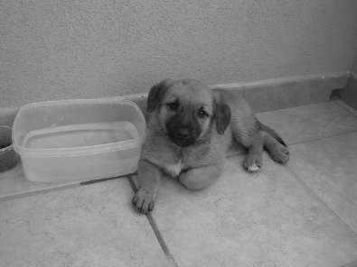
(a)	(b)

Figure 3: A black and white image (a) and its grey scales distribution (b).

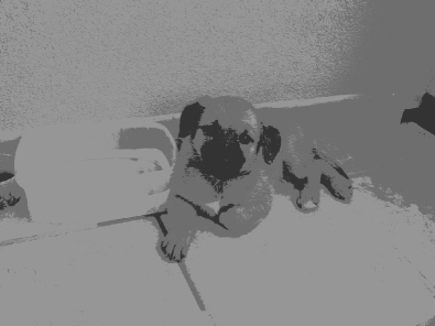
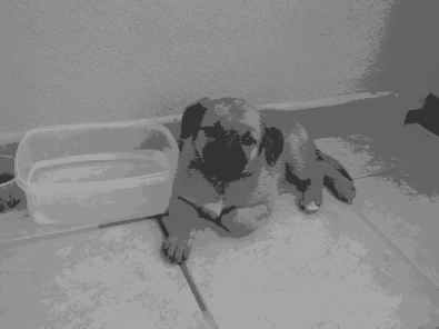
Figure 4: Color quantization via MFG clustering (left panels) and the corresponding mixtures (right panels), for $K=2,3,5$ (from top to bottom panels).

Test 4. We finally consider a two dimensional example. We take some data from the Elki project [16], forming a “mouse” similar to a popular comic character. The data set is organized in $3$ clusters (plus some random noise), corresponding to the head and the ears of the mouse, see Figure 5. Then, we set $K=3$, we discretize the domain $\Omega=[0,1]^{2}$ by means of a uniform grid of $N=51^{2}$ nodes, and we build the distribution $f$ as in the previous test, by counting the data points falling in each cell of the grid and normalizing the result to obtain $\int_{\Omega}f(x)\,dx=1$. For the visual representation, we consider RGB triplets in $[0,1]^{3}$, and we assign to the three clusters the pure colors red $(1,0,0)$, green $(0,1,0)$ and blue $(0,0,1)$ respectively. Then we use the responsibilities $\{\gamma_{k}\}_{k=1,2,3}\in[0,1]$ to compute the color of each cell of the grid as $C_{i}=(\gamma_{1}(x_{i}),\gamma_{2}(x_{i}),\gamma_{3}(x_{i}))$, for $i=1,...,N$, which quantifies how much it belongs to a certain cluster. Figure 6 shows the surface of the computed mixture and the corresponding clusterization. We observe that the scattered data set is well approximated by the mixture, and the corresponding three clusters are well separated by small overlapping regions.

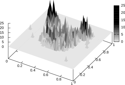
(a)	(b)

Figure 5: The “mouse” data set (a) and the corresponding distribution (b).

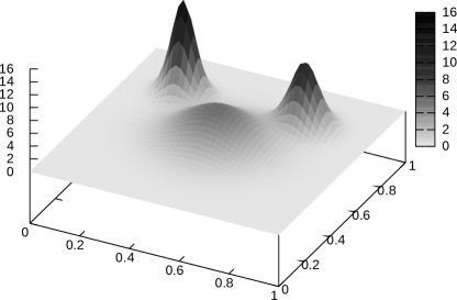
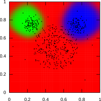
(a)	(b)

Figure 6: MFG mixture (a) and clustering (b) of the “mouse” data set for $K=3$.

laura.aquilanti@sbai.uniroma1.it
fabio.camilli@sbai.uniroma1.it
SBAI, Sapienza Università di Roma
via A.Scarpa 14, 00161 Roma (Italy)

cacace@mat.uniroma3.it
Dipartimento di Matematica e Fisica
Università degli Studi Roma Tre
Largo S. L. Murialdo 1, 00146 Roma (Italy)

r.demaio@iconsulting.biz
IConsulting
Via della Conciliazione 10, 00193 Roma (Italy)

References

- [1] Y. Achdou and I. Capuzzo Dolcetta, Mean Field Games: numerical methods, SIAM J. Numer. Anal., 48 (2010), pp. 1136–1162.
- [2] N. Almulla, R. Ferreira and D. Gomes, Two numerical approaches to stationary mean-field games, Dyn. Games Appl. 7 (2017), no. 4, 657–682.
- [3] M. Bardi and F. Priuli, Linear-quadratic N-person and mean-field games with ergodic cost, SIAM J. Control Optim. 52 (2014), no. 5, 3022–3052.
- [4] A. Bensoussan, Perturbation methods in optimal control, Wiley/Gauthier-Villars Series in Modern Applied Mathematics, 1988.
- [5] C. Bertucci, S. Vassilaras, J.-M. Lasry, G. Paschos, M. Debbah and P.-L. Lions, Transmit strategies for massive machine-type communications based on Mean Field Games, in Proceedings of the International Symposium on Wireless Communication System (ISWCS), 2018.
- [6] C.M. Bishop, Pattern recognition and Machine Learning, Information Science and Statistics, Springer, New York, 2006.
- [7] J.A. Bilmes, A gentle tutorial of the EM algorithm and its application to parameter estimation for Gaussian mixture and hidden Markov model, Technical Report ICSI-TR-97-021, University of Berkeley, 2000.
- [8] L. Bottou and Y. Bengio, Convergence properties of the K-means algorithms, Adv. Neural Inf. Process. Syst. 82 (1995), 585-592.
- [9] S. Cacace and F. Camilli, A generalized Newton method for homogenization of Hamilton-Jacobi equations, SIAM J. Sci. Comput. 38 (2016), no. 6, A3589-A3617.
- [10] E. Carlini and F.J. Silva, On the discretization of some nonlinear Fokker-Planck-Kolmogorov equations and applications. SIAM J. Numer. Anal. 56 (2018), no. 4, 2148–2177.
- [11] P. Chaudhari, A. Oberman, S. Osher, S. Soatto and G. Carlier, Deep relaxation: partial differential equations for optimizing deep neural networks, Res. Math. Sci. 5 (2018), no. 3, Paper No. 30, 30 pp.
- [12] Y. Chen, T. T. Georgiou and A. Tannenbaum, Optimal Transport for Gaussian Mixture Models, in IEEE Access, vol. 7, pp. 6269-6278, 2019
- [13] M. Cirant, Multi-population Mean Field Games systems with Neumann boundary conditions. J. Math. Pures Appl. 103 (2015), no. 5, 1294–1315.
- [14] J.L. Coron, Quelques exemples de jeux à champ moyen, Ph.D. thesis, Université Paris-Dauphine, 2018.
- [15] W. E, J. Han and Q. Li, A mean-field optimal control formulation of deep learning. Res. Math. Sci. 6 (2019), no. 1, Paper No. 10, 41 pp.
- [16] https://elki-project.github.io/datasets/
- [17] D. Gilbarg and N.S.Trudinger, Elliptic partial differential equations of second order, Classics in Mathematics. Springer-Verlag, Berlin, 2001.
- [18] O. Guéant, J-M. Lasry and P-L. Lions, Mean Field Games and applications, in Paris-Princeton Lectures on Mathematical Finance 2010, Lecture Notes in Math., 2003, Springer, Berlin, 2011, 205–266.
- [19] J.-M. Lasry and P.-L. Lions, Mean Field Games. Jpn. J. Math., 2 (2007), 229-260.
- [20] P.-L. Lions, Quelques remarques sur les problemes elliptiques quasilineaires du second ordre, J. Anal. Math 45 (1985) 234-254.
- [21] S. Miyiamoto and M. Mukaidono, Fuzzy C-Means as a regularization and maximum entropy approach. IFSA’97 Prague: Proceedings [of the] seventh International Fuzzy Systems Association World Congress, 86-92.
- [22] S. Pequito, A.P. Aguiar, B. Sinopoli and D. Gomes, Unsupervised learning of finite mixture models using Mean Field Games, in Annual Allerton Conference on Communication, Control and Computing, 2011, 321-328.
- [23] A. Saxena, M. Prasad, A. Gupta, N. Bharill, O.P. Patel, A. Tiwari, M.J. Er, W. Ding and C.T. Lin, A review of clustering techniques and developments, Neurocomputing, 267 (2017), 664–681.