Learning a Domain-Invariant Embedding for Unsupervised Domain Adaptation Using Class-Conditioned Distribution Alignment

Abstract

We address the problem of unsupervised domain adaptation (UDA) by learning a cross-domain agnostic embedding space, where the distance between the probability distributions of the two source and target visual domains is minimized. We use the output space of a shared cross-domain deep encoder to model the embedding space and use the Sliced-Wasserstein Distance (SWD) to measure and minimize the distance between the embedded distributions of two source and target domains to enforce the embedding to be domain-agnostic. Additionally, we use the source domain labeled data to train a deep classifier from the embedding space to the label space to enforce the embedding space to be discriminative. As a result of this training scheme, we provide an effective solution to train the deep classification network on the source domain such that it will generalize well on the target domain, where only unlabeled training data is accessible. To mitigate the challenge of class matching, we also align corresponding classes in the embedding space by using high confidence pseudo-labels for the target domain, i.e. assigning the class for which the source classifier has a high prediction probability. We provide experimental results on UDA benchmark tasks to demonstrate that our method is effective and leads to state-of-the-art performance.

I Introduction

Deep learning classification algorithms have surpassed performance of humans for a wide range of computer vision applications. However, this achievement is conditioned on availability of high-quality labeled datasets to supervise training deep neural networks. Unfortunately, preparing huge labeled datasets is not feasible for many situations as data labeling and annotation can be expensive [29]. Domain adaptation [12] is a paradigm to address the problem of labeled data scarcity in computer vision, where the goal is to improve learning speed and model generalization as well as to avoid expensive redundant model retraining. The major idea is to overcome labeled data scarcity in a target domain by transferring knowledge from a related auxiliary source domain, where labeled data is easy and cheap to obtain.

A common technique in domain adaptation literature is to embed data from the two source and target visual domains in an intermediate embedding space such that common cross-domain discriminative relations are captured in the embedding space. For example, if the data from source and target domains have similar class-conditioned probability distributions in the embedding space, then a classifier trained solely using labeled data from the source domain will generalize well on data points that are drawn from the target domain distribution [28, 30].

In this paper, we propose a novel unsupervised adaptation (UDA) algorithm following the above explained procedure. Our approach is a simpler, yet effective, alternative for adversarial learning techniques that have been more dominant to address probability matching indirectly for UDA [41, 43, 23]. Our contribution is two folds. First, we train the shared encoder by minimizing the Sliced-Wasserstein Distance (SWD) [26] between the source and the target distributions in the embedding space. We also train a classifier network simultaneously using the source domain labeled data. A major benefit of SWD over alternative probability metrics is that it can be computed efficiently. Additionally, SWD is known to be suitable for gradient-based optimization which is essential for deep learning [28]. Our second contribution is to circumvent the class matching challenge [34] by minimizing SWD between conditional distributions in sequential iterations for better performance compared to prior UDA methods that match probabilities explicitly. At each iteration, we assign pseudo-labels only to the target domain data that the classifier predicts the assigned class label with high probability and use this portion of target data to minimize the SWD between conditional distributions. As more learning iterations are performed, the number of target data points with correct pseudo-labels grows and progressively enforces distributions to align class-conditionally. We provide experimental results on benchmark problems, including ablation and sensitivity studies, to demonstrate that our method is effective.

II Background and Related Work

There are two major approaches in the literature to address domain adaption. The approach for a group of methods is based on preprocessing the target domain data points. The target data is mapped from the target domain to the source domain such that the target data structure is preserved in the source [33]. Another common approach is to map data from both domains to a latent domain invariant space [7]. Early methods within the second approach learn a linear subspace as the invariant space  [15, 13] where the target domain data points distribute similar to the source domain data points. A linear subspace is not suitable for capturing complex distributions. For this reason, recently deep neural networks have been used to model the intermediate space as the output of the network. The network is trained such that the source and the target domain distributions in its output possess minimal discrepancy. Training procedure can be done both by adversarial learning [14] or directly minimizing the distance between the two distributions [4].

Several important UDA methods use adversarial learning. Ganin et al. [10] pioneered and developed an effective method to match two distributions indirectly by using adversarial learning. Liu et al. [21] and Tzeng et al. [41] use the Generative Adversarial Networks (GAN) structure [14] to tackle domain adaptation. The idea is to train two competing (i.e., adversarial) deep neural networks to match the source and the target distributions. A generator network maps data points from both domains to the domain-invariant space and a binary discriminator network is trained to classify the data points, with each domain considered as a class, based on the representations of the target and the source data points. The generator network is trained such that eventually the discriminator cannot distinguish between the two domains, i.e. classification rate becomes $50\%$.

A second group of domain adaptation algorithms match the distributions directly in the embedding by using a shared cross-domain mapping such that the distance between the two distributions is minimized with respect to a distance metric [4]. Early methods use simple metrics such the Maximum Mean Discrepancy (MMD) for this purpose [16]. MMD measures the distances between the distance between distributions simply as the distance between the mean of embedding features. In contrast, more recent techniques that use a shared deep encoder, employ the Wasserstein metric [42] to address UDA [4, 6]. Wasserstein metric is shown to be a more accurate probability metric and can be minimized effectively by deep learning first-order optimization techniques. A major benefit of matching distributions directly is existence of theoretical guarantees. In particular, Redko et al. [28] provided theoretical guarantees for using a Wasserstein metric to address domain adaptation. Additionally, adversarial learning often requires deliberate architecture engineering, optimization initialization, and selection of hyper-parameters to be stable [32]. In some cases, adversarial learning also suffers from a phenomenon known as mode collapse [22]. That is, if the data distribution is a multi-modal distribution, which is the case for most classification problems, the generator network might not generate samples from some modes of the distribution. These challenges are easier to address when the distributions are matched directly.

As Wasserstein distance is finding more applications in deep learning, efficient computation of Wasserstein distance has become an active area of research. The reason is that Wasserstein distance is defined in form of a linear programming optimization and solving this optimization problem is computationally expensive for high-dimensional data. Although computationally efficient variations and approximations of the Wasserstein distance have been recently proposed [5, 40, 25], these variations still require an additional optimization in each iteration of the stochastic gradient descent (SGD) steps to match distributions. Courty et al. [4] used a regularized version of the optimal transport for domain adaptation. Seguy et al. [36] used a dual stochastic gradient algorithm for solving the regularized optimal transport problem. Alternatively, we propose to address the above challenges using Sliced Wasserstein Distance (SWD). Definition of SWD is motivated by the fact that in contrast to higher dimensions, the Wasserstein distance for one-dimensional distributions has a closed form solution which can be computed efficiently. This fact is used to approximate Wasserstein distance by SWD, which is a computationally efficient approximation and has recently drawn interest from the machine learning and computer vision communities [26, 1, 3, 8, 39].

III Problem Formulation

Consider a source domain, $\mathcal{D}_{\mathcal{S}}=(\bm{X}_{\mathcal{S}},\bm{Y}_{\mathcal{S}})$, with $N$ labeled samples, i.e. labeled images, where $\bm{X}_{\mathcal{S}}=[\bm{x}_{1}^{s},\ldots,\bm{x}_{N}^{s}]\in\mathcal{X}\subset\mathbb{R}^{d\times N}$ denotes the samples and $\bm{Y}_{\mathcal{S}}=[\mathbf{y}^{s}_{1},...,\mathbf{y}^{s}_{N}]\in\mathcal{Y}\subset\mathbb{R}^{k\times N}$ contains the corresponding labels. Note that label $\mathbf{y}^{s}_{n}$ identifies the membership of $\bm{x}^{s}_{n}$ to one or multiple of the $k$ classes (e.g. digits $1,...,10$ for hand-written digit recognition). We assume that the source samples are drawn i.i.d. from the source joint probability distribution, i.e. $(\bm{x}_{i}^{s},\bm{y}_{i})\sim p(\bm{x}^{\mathcal{S}},y)$. We denote the source marginal distribution over $\bm{x}^{\mathcal{S}}$ with $p_{S}$. Additionally, we have a related target domain (e.g. machine-typed digit recognition) with $M$ unlabeled data points $\bm{X}_{\mathcal{T}}=[\bm{x}_{1}^{t},\ldots,\bm{x}_{M}^{t}]\in\mathbb{R}^{d\times M}$. Following existing UDA methods, we assume that the same type of labels in the source domain holds for the target domain. The target samples are drawn from the target marginal distribution $\bm{x}_{i}^{t}\sim p_{T}$. We also know that despite similarity between these domains, distribution discrepancy exists between these two domains, i.e. $p_{S}\neq p_{T}$. Our goal is to classify the unlabeled target data points through knowledge transfer from the source domain. Learning a good classifier for the source data points is a straight forward problem as given a large enough number of source samples, $N$, a parametric function $f_{\theta}:\mathbb{R}^{d}\rightarrow\mathcal{Y}$, e.g., a deep neural network with concatenated learnable parameters $\theta$, can be trained to map samples to their corresponding labels using standard supervised learning solely in the source domain. The training is conducted via minimizing the empirical risk, $\hat{\theta}=\arg\min_{\theta}\hat{e}_{\theta}=\arg\min_{\theta}\sum_{i}\mathcal{L}(f_{\theta}(\bm{x}_{i}^{s}),\bm{y}_{i}^{s})$, with respect to a proper loss function, $\mathcal{L}(\cdot)$ (e.g., cross entropy loss). The learned classifier $f_{\hat{\theta}}$ generalizes well on testing data points if they are drawn from the training data point’s distributions. Only then, the empirical risk is a suitable surrogate for the real risk function, $e=\mathbb{E}_{(\bm{x},y)\sim p(\bm{x}^{\mathcal{S}},y^{\mathcal{S}})}(\mathcal{L}(f_{\theta}(\bm{x}),y))$. Hence the naive approach of using $f_{\hat{\theta}}$ on the target domain might not be effective as given the discrepancy between the source and target distributions, $f_{\hat{\theta}}$ might not generalize well on the target domain. Therefore, there is a need for adapting the training procedure of $f_{\hat{\theta}}$ by incorporating unlabeled target data points such that the learned knowledge from the source domain could be transferred and used for classification in the target domain using only the unlabeled samples.

The main challenge is to circumvent the problem of discrepancy between the source and the target domain distributions. To that end, the mapping $f_{\theta}(\cdot)$ can be decomposed into a feature extractor $\phi_{\bm{v}}(\cdot)$ and a classifier $h_{\bm{w}}(\cdot)$, such that $f_{\theta}=h_{\bm{w}}\circ\phi_{\bm{v}}$, where $\bm{w}$ and $\bm{v}$ are the corresponding learnable parameters, i.e. $\theta=(\bm{w},\bm{v})$. The core idea is to learn the feature extractor function, $\phi_{\bm{v}}$, for both domains such that the domain specific distribution of the extracted features to be similar to one another. The feature extracting function $\phi_{\bm{v}}:\mathcal{X}\rightarrow\mathcal{Z}$, maps the data points from both domains to an intermediate embedding space $\mathcal{Z}\subset\mathbb{R}^{f}$ (i.e., feature space) and the classifier $h_{\bm{w}}:\mathcal{Z}\rightarrow\mathcal{Y}$ maps the data points representations in the embedding space to the label set. Note that, as a deterministic function, the feature extractor function $\phi_{\bm{v}}$ can change the distribution of the data in the embedding. Therefore, if $\phi_{\bm{v}}$ is learned such that the discrepancy between the source and target distributions is minimized in the embedding space, i.e., discrepancy between $p_{\mathcal{S}}(\phi(\bm{x}^{s}))$ and $p_{\mathcal{T}}(\phi(\bm{x}^{t}))$ (i.e., the embedding is domain agnostic), then the classifier would generalize well on the target domain and could be used to label the target domain data points. This is the core idea behind various prior domain adaptation approaches in the literature [24, 11].

IV Proposed Method

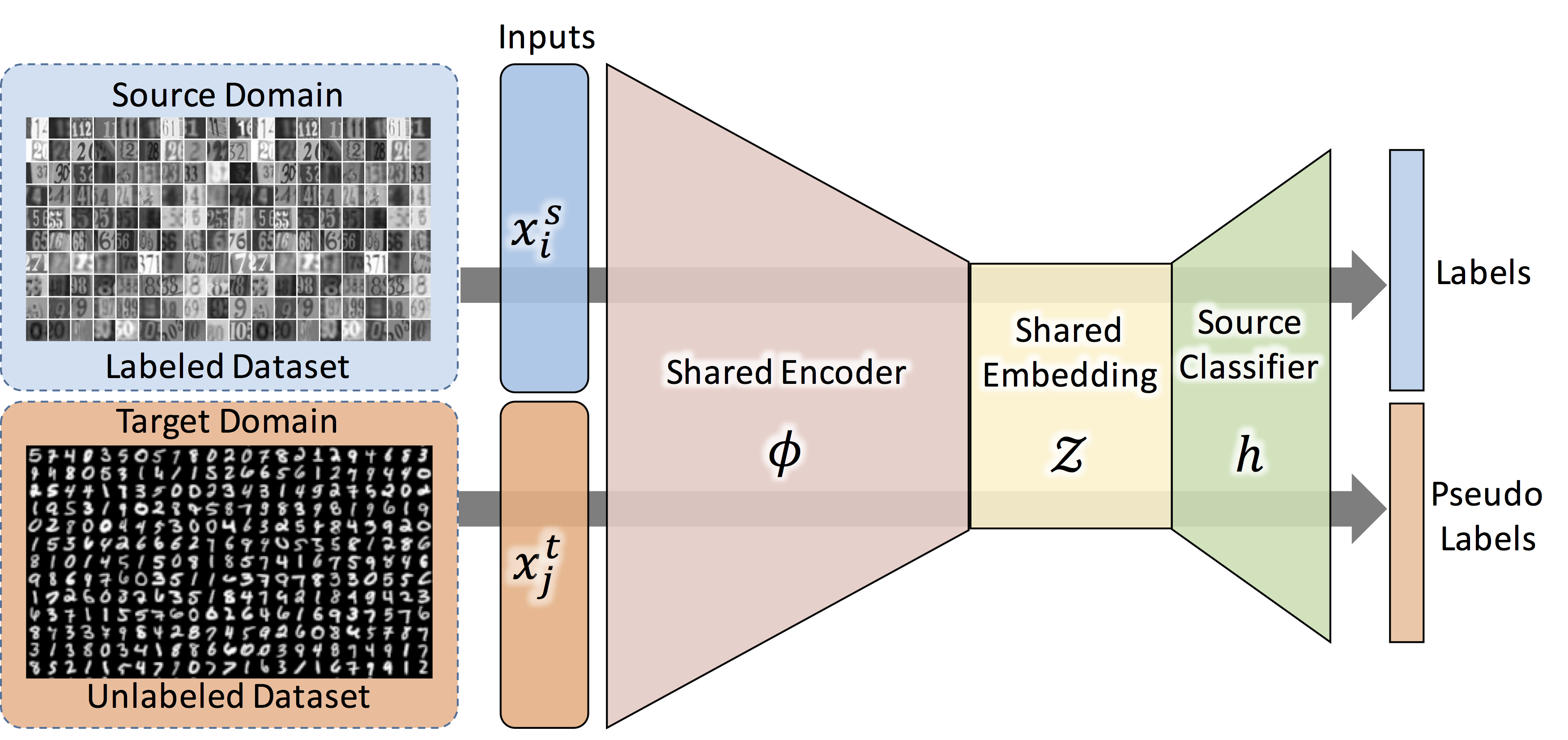
Figure 1: Architecture of the proposed unsupervised domain adaptation framework.

We consider the case where the feature extractor, $\phi_{\bm{v}}(\cdot)$, is a deep convolutional encoder with weights $\bm{v}$ and the classifier $h_{\bm{w}}(\cdot)$ is a shallow fully connected neural network with weights $\bm{w}$. The last layer of the classifier network is a softmax layer that assigns a membership probability distribution to any given data point. It is often the case that the labels of data points are assigned according to the class with maximum predicted probability. In short, the encoder network is learned to mix both domains such that the extracted features in the embedding are: 1) domain agnostic in terms of data distributions, and 2) discriminative for the source domain to make learning $h_{\bm{w}}$ feasible. Figure 1 demonstrates system level presentation of our framework. Following this framework, the UDA reduces to solving the following optimization problem to solve for $\bm{v}$ and $\bm{w}$:

$$\begin{split}\min_{\bm{v},\bm{w}}&\sum_{i=1}^{N}\mathcal{L}\big{(}h_{\bm{w}}(\phi_{\bm{v}}(\bm{x}_{i}^{s})),\bm{y}_{i}^{s}\big{)}\\ &+\lambda D\big{(}p_{\mathcal{S}}(\phi_{\bm{v}}(\bm{X}_{\mathcal{S}})),p_{\mathcal{T}}(\phi_{\bm{v}}(\bm{X}_{\mathcal{T}}))\big{)},\end{split}$$ (1)

where $D(\cdot,\cdot)$ is a discrepancy measure between the probabilities and $\lambda$ is a trade-off parameter. The first term in Eq. (1) is empirical risk for classifying the source labeled data points from the embedding space and the second term is the cross-domain probability matching loss. The encoder’s learnable parameters are learned using data points from both domains and the classifier parameters are simultaneously learned using the source domain labeled data.

A major remaining question is to select a proper metric. First, note that the actual distributions $p_{\mathcal{S}}(\phi(\bm{X}_{\mathcal{S}}))$ and $p_{\mathcal{T}}(\phi(\bm{X}_{\mathcal{T}}))$ are unknown and we can rely only on observed samples from these distributions. Therefore, a sensible discrepancy measure, $D(\cdot,\cdot)$, should be able to measure the dissimilarity between these distributions only based on the drawn samples. In this work, we use the SWD [27] as it is computationally efficient to compute SWD from drawn samples from the corresponding distributions. More importantly, the SWD is a good approximation for the optimal transport [2] which has gained interest in deep learning community as it is an effective distribution metric and its gradient is non-vanishing.

The idea behind the SWD is to project two $d$-dimensional probability distributions into their marginal one-dimensional distributions, i.e., slicing the high-dimensional distributions, and to approximate the Wasserstein distance by integrating the Wasserstein distances between the resulting marginal probability distributions over all possible one-dimensional subspaces. For the distribution $p_{\mathcal{S}}$, a one-dimensional slice of the distribution is defined as:

$$\mathcal{R}p_{\mathcal{S}}(t;\gamma)=\int_{\mathcal{S}}p_{\mathcal{S}}(\bm{x})\delta(t-\langle\gamma,\bm{x}\rangle)d\bm{x},$$ (2)

where $\delta(\cdot)$ denotes the Kronecker delta function, $\langle\cdot,\cdot\rangle$ denotes the vector dot product, $\mathbb{S}^{d-1}$ is the $d$-dimensional unit sphere and $\gamma$ is the projection direction. In other words, $\mathcal{R}p_{\mathcal{S}}(\cdot;\gamma)$ is a marginal distribution of $p_{\mathcal{S}}$ obtained from integrating $p_{\mathcal{S}}$ over the hyperplanes orthogonal to $\gamma$. The SWD then can be computed by integrating the Wasserstein distance between sliced distributions over all $\gamma$:

$$SW(p_{\mathcal{S}},p_{\mathcal{T}})=\int_{\mathbb{S}^{d-1}}W(\mathcal{R}p_{\mathcal{S}}(\cdot;\gamma),\mathcal{R}p_{\mathcal{T}}(\cdot;\gamma))d\gamma$$ (3)

where $W(\cdot)$ denotes the Wasserstein distance. The main advantage of using the SWD is that, unlike the Wasserstein distance, calculation of the SWD does not require a numerically expensive optimization. This is due to the fact that the Wasserstein distance between two one-dimensional probability distributions has a closed form solution and is equal to the $\ell_{p}$-distance between the inverse of their cumulative distribution functions Since only samples from distributions are available, the one-dimensional Wasserstein distance can be approximated as the $\ell_{p}$-distance between the sorted samples [31]. The integral in Eq. (3) is approximated using a Monte Carlo style numerical integration. Doing so, the SWD between $f$-dimensional samples $\{\phi(\mathbf{x}_{i}^{\mathcal{S}})\in\mathbb{R}^{f}\sim p_{\mathcal{S}}\}_{i=1}^{M}$ and $\{\phi(\mathbf{x}_{i}^{\mathcal{T}})\in\mathbb{R}^{f}\sim p_{\mathcal{T}}\}_{j=1}^{M}$ can be approximated as the following sum:

$$SW^{2}(p_{\mathcal{S}},p_{\mathcal{T}})\approx\frac{1}{L}\sum_{l=1}^{L}\sum_{i=1}^{M}|\langle\gamma_{l},\phi(\mathbf{x}_{s_{l}[i]}^{\mathcal{S}}\rangle)-\langle\gamma_{l},\phi(\mathbf{x}_{t_{l}[i]}^{\mathcal{T}})\rangle|^{2}$$ (4)

where $\gamma_{l}\in\mathbb{S}^{f-1}$ is uniformly drawn random sample from the unit $f$-dimensional ball $\mathbb{S}^{f-1}$, and $s_{l}[i]$ and $t_{l}[i]$ are the sorted indices of $\{\gamma_{l}\cdot\phi(\mathbf{x}_{i})\}_{i=1}^{M}$ for source and target domains, respectively. Note that for a fixed dimension $d$, Monte Carlo approximation error is proportional to $O(\frac{1}{\sqrt{L}})$. We utilize the SWD as the discrepancy measure between the probability distributions to match them in the embedding space. Next, we discuss a major deficiency in Eq. (1) and our remedy to tackle it. We utilize the SWD as the discrepancy measure between the probability densities, $p_{\mathcal{S}}(\phi(\bm{x}_{\mathcal{S}})|C_{j})\big{)}$ and $p_{\mathcal{T}}(\phi(\bm{x}_{\mathcal{T}})|C_{j})\big{)}$.

IV-A Class-conditional Alignment of Distributions

A main shortcoming of Eq. (1) is that minimizing the discrepancy between $p_{\mathcal{S}}(\phi(\bm{X}_{\mathcal{S}}))$ and $p_{\mathcal{T}}(\phi(\bm{X}_{\mathcal{T}}))$ does not guarantee semantic consistency between the two domains. To clarify this point, consider the source and target domains to be images corresponding to printed digits and handwritten digits. While the feature distributions in the embedding space could have low discrepancy, the classes might not be correctly aligned in this space, e.g. digits from a class in the target domain could be matched to a wrong class of the source domain or, even digits from multiple classes in the target domain could be matched to the cluster of a single digit of the source domain. In such cases, the source classifier will not generalize well on the target domain. In other words, the shared embedding space, $\mathcal{Z}$, might not be a semantically meaningful space for the target domain if we solely minimize SWD between $p_{\mathcal{S}}(\phi(\bm{X}_{\mathcal{S}}))$ and $p_{\mathcal{T}}(\phi(\bm{X}_{\mathcal{T}}))$. To solve this challenge, the encoder function should be learned such that the class-conditioned probabilities of both domains in the embedding space are similar, i.e. $p_{\mathcal{S}}(\phi(\bm{x}_{\mathcal{S}})|C_{j})\approx p_{\mathcal{T}}(\phi(\bm{x}_{\mathcal{T}})|C_{j})$, where $C_{j}$ denotes a particular class. Given this, we can mitigate the class matching problem by using an adapted version of Eq. (1) as:

$$\begin{split}\min_{\bm{v},\bm{w}}&\sum_{i=1}^{N}\mathcal{L}\big{(}h_{\bm{w}}(\phi_{\bm{v}}(\bm{x}_{i}^{s})),\bm{y}_{i}^{s}\big{)}\\ &+\lambda\sum_{j=1}^{k}D\big{(}p_{\mathcal{S}}(\phi_{\bm{v}}(\bm{x}_{\mathcal{S}})|C_{j}),p_{\mathcal{T}}(\phi_{\bm{v}}(\bm{x}_{\mathcal{T}})|C_{j})\big{)},\end{split}$$ (5)

where discrepancy between distributions is minimized conditioned on classes, to enforce semantic alignment in the embedding space. Solving Eq. (5), however, is not tractable as the labels for the target domain are not available and the conditional distribution, $p_{\mathcal{T}}(\phi(\bm{x}_{\mathcal{T}})|C_{j})\big{)}$, is not known.

Algorithm 1 $\mathrm{DACAD}\left(L,\eta,\lambda\right)$

1:Input: data $\mathcal{D}_{\mathcal{S}}=(\bm{X}_{\mathcal{S}},\bm{Y}_{\mathcal{S}});\mathcal{D}_{\mathcal{T}}=(\bm{X}_{\mathcal{S}})$,

2:Pre-training:

3:     $\hat{\theta}_{0}=(\bm{w}_{0},\bm{v}_{0})=\arg\min_{\theta}\sum_{i}\mathcal{L}(f_{\theta}(\bm{x}_{i}^{s}),\bm{y}_{i}^{s})$

4:for $itr=1,\ldots,ITR$  do

5:    $\mathcal{D}_{\mathcal{PL}}=\{(\bm{x}_{i}^{t},\hat{\bm{y}}_{i}^{t})|\hat{\bm{y}}_{i}^{t}=f_{\hat{\theta}}(\bm{x}_{i}^{t}),p(\hat{\bm{y}}_{i}^{t}|\bm{x}_{i}^{t})>\tau\}$

6:    for  $alt=1,\ldots,ALT$  do

7:         Update encoder parameters using pseudo-labels:

8:              $\hat{\bm{v}}=\sum_{j}D\big{(}p_{\mathcal{S}}(\phi_{\bm{v}}(\bm{x}_{\mathcal{S}})|C_{j}),p_{\mathcal{SL}}(\phi_{\bm{v}}(\bm{x}_{\mathcal{T}})|C_{j})\big{)}$

9:         Update entire model:

10:              $\hat{\bm{v}},\hat{\bm{w}}=\arg\min_{\bm{w},\bm{v}}\sum_{i=1}^{N}\mathcal{L}\big{(}h_{\bm{w}}(\phi_{\hat{\hat{\bm{v}}}}(\bm{x}_{i}^{s})),\bm{y}_{i}^{s}\big{)}$

11:    end for

12:end for

To tackle the above issue, we compute a surrogate of the objective in Eq. (5). Our idea is to approximate $p_{\mathcal{T}}(\phi(\bm{x}_{\mathcal{T}})|C_{j})\big{)}$ by generating pseudo-labels for the target data points. The pseudo-labels are obtained from the source classifier prediction, but only for the portion of target data points that the the source classifier provides confident prediction. More specifically, we solve Eq. (5) in incremental gradient descent iterations. In particular, we first initialize the classifier network by training it on the source data. We then alternate between optimizing the classification loss for the source data and SWD loss term at each iteration. At each iteration, we pass the target domain data points into the classifier learned on the source data and analyze the label probability distribution on the softmax layer of the classifier. We choose a threshold $\tau$ and assign pseudo-labels only to those target data points that the classifier predicts the pseudo-labels with high confidence, i.e. $p(\bm{y}_{i}|\bm{x}_{i}^{t})>\tau$. Since the source and the target domains are related, it is sensible that the source classifier can classify a subset of target data points correctly and with high confidence. We use these data points to approximate $p_{\mathcal{T}}(\phi(\bm{x}_{\mathcal{T}})|C_{j})\big{)}$ in Eq. (5) and update the encoder parameters, $\bm{v}$, accordingly. In our empirical experiments, we have observed that because the domains are related, as more optimization iterations are performed, the number of data points with confident pseudo-labels increases and our approximation for Eq. (5) improves and becomes more stable, enforcing the source and the target distributions to align class conditionally in the embedding space. As a side benefit, since we math the distributions class-conditionally, a problem similar to mode collapse is unlikely to occur. Figure 2 visualizes this process using real data. Our proposed framework, named Domain Adaptation with Conditional Alignment of Distributions (DACAD) is summarized in Algorithm 1.

V Experimental Validation

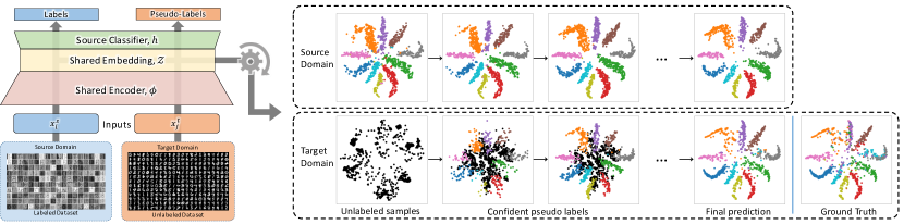
Figure 2: The high-level system architecture, shown on the left, illustrates the data paths used during UDA training. On the right, t_SNE visualizations demonstrate how the embedding space evolves during training for the $\mathcal{S}\rightarrow\mathcal{U}$ task. In the target domain, colored points are examples with assigned pseudo-labels, which increase in number with the confidence of the classifier.

We evaluate our algorithm using standard benchmark UDA tasks and compare against several UDA methods.

Datasets: We investigate the empirical performance of our proposed method on five commonly used benchmark datasets in UDA, namely: MNIST ($\mathcal{M}$) [19], USPS ($\mathcal{U}$) [20], Street View House Numbers, i.e., SVHN ($\mathcal{S}$), CIFAR ($\mathcal{CI}$), and STL ($\mathcal{ST}$). The first three datasets are 10 class (0-9) digit classification datasets. MNIST and USPS are collection of hand written digits whereas SVHN is a collection of real world RGB images of house numbers. STL and CIFAR contain RGB images that share 9 object classes: airplane, car, bird, cat, deer, dog, horse, ship, and truck. For the digit datasets, while six domain adaptation problems can be defined among these datasets, prior works often consider four of these six cases, as knowledge transfer from simple MNIST and USPS datasets to a more challenging SVHN domain does not seem to be tractable. Following the literature, we use 2000 randomly selected images from MNIST and 1800 images from USPS in our experiments for the case of $\mathcal{U}\rightarrow\mathcal{M}$ and $\mathcal{S}\rightarrow\mathcal{M}$ [23]. In the remaining cases, we used full datasets. All datasets have their images scaled to $32\times 32$ pixels and the SVHN images are converted to grayscale as the encoder network is shared between the domains. CIFAR and STL maintain their RGB components. We report the target classification accuracy across the tasks.

Pre-training: Our experiments involve a pre-training stage to initialize the encoder and the classifier networks solely using the source data. This is an essential step because the combined deep network can generate confident pseudo-labels on the target domain only if initially trained on the related source domain. In other words, this initially learned network can be served as a naive model on the target domain. We then boost the performance on the target domain using our proposed algorithm, demonstrating that our algorithm is indeed effective for transferring knowledge. Doing so, we investigate a less-explored issue in the UDA literature. Different UDA approaches use considerably different networks, both in terms of complexity, e.g. number of layers and convolution filters, and the structure, e.g. using an auto-encoder. Consequently, it is ambiguous whether performance of a particular UDA algorithm is due to successful knowledge transfer from the source domain or just a good baseline network that performs well on the target domain even without considerable knowledge transfer from the source domain. To highlight that our algorithm can indeed transfer knowledge, we use two different network architectures: DRCN [11] and VGG [38]. We then show that our algorithm can effectively boost base-line performance (statistically significant) regardless of the underlying network. In most of the domain adaptation tasks, we demonstrate that this boost indeed stems from transferring knowledge from the source domain. In our experiments we used Adam optimizer  [18] and set the pseudo-labeling threshold to $tr=0.99$.

Method	$\mathcal{M}\rightarrow\mathcal{U}$	$\mathcal{U}\rightarrow\mathcal{M}$	$\mathcal{S}\rightarrow\mathcal{M}$	$\mathcal{S}\rightarrow\mathcal{U}$	$\mathcal{ST}\rightarrow\mathcal{CI}$	$\mathcal{CI}\rightarrow\mathcal{ST}$
GtA	92.8$\pm$0.9	90.8$\pm$1.3	92.4$\pm$0.9	-	-	-
CoGAN	91.2$\pm$0.8	89.1$\pm$0.8	-	-	-	-
ADDA	89.4$\pm$0.2	90.1$\pm$0.8	76.0$\pm$1.8	-	-	-
CyCADA	95.6$\pm$0.2†	96.5$\pm$0.1†	90.4$\pm$0.4	-	-	-
I2I-Adapt	92.1†	87.2†	80.3	-	-	-
FADA	89.1	81.1	72.8	78.3	-	-
RevGrad	77.1$\pm$1.8‡	73.0$\pm$2.0‡	73.9	-	-	-
DRCN	91.8$\pm$0.1†	73.7$\pm$0.04†	82.0$\pm$0.2	-	58.9$\pm$0.1	66.4$\pm$0.1
AUDA	-	-	86.0	-	-	-
OPDA	70.0	60.2	-	-	-	-
MML	77.9†	60.5†	62.9	-	-	-
Target (FS)	96.8$\pm$0.2	98.5$\pm$0.2	98.5$\pm$0.2	96.8$\pm$0.2	81.5$\pm$1.0	64.8$\pm$1.7
VGG	90.1$\pm$2.6	80.2$\pm$5.7	67.3$\pm$2.6	66.7$\pm$2.7	53.8$\pm$1.4	63.4$\pm$1.2
DACAD	92.4$\pm$1.2	91.1$\pm$3.0	80.0$\pm$2.7	79.6$\pm$3.3	54.4$\pm$1.9	66.5$\pm$1.0
DACAD	93.6$\pm$1.0	95.8$\pm$1.3	82.0$\pm$3.4	78.0$\pm$2.0	44.4$\pm$0.4	65.7$\pm$1.0
DRCN (Ours)	88.6$\pm$1.3	89.6$\pm$1.3	74.3$\pm$2.8	54.9$\pm$1.8	50.0$\pm$1.5	64.2$\pm$1.7
DACAD	94.5$\pm$0.7	97.7$\pm$0.3	88.2$\pm$2.8	82.6$\pm$2.9	55.0$\pm$1.4	65.9$\pm$1.4

TABLE I: Classification accuracy for UDA between MINIST, USPS, SVHN, CIFAR, and STL datasets. ^† indicates use of full MNIST and USPS datasets as opposed to the subset described in the paper. ^‡ indicates results from reimplementation in  [41].

Data Augmentation: Following the literature, we use data augmentation to create additional training data by applying reasonable transformations to input data in an effort to improve generalization [37]. Confirming the reported result in [11], we also found that geometric transformations and noise, applied to appropriate inputs, greatly improves performance and transferability of the source model to the target data. Data augmentation can help to reduce the domain shift between the two domains. The augmentations in this work are limited to translation, rotation, skew, zoom, Gaussian noise, Binomial noise, and inverted pixels.

V-A Results

Figure 2 demonstrates how our algorithm successfully learns an embedding with class-conditional alignment of distributions of both domains. This figure presents the two-dimensional t_SNE visualization of the source and target domain data points in the shared embedding space for the $\mathcal{S}\rightarrow\mathcal{U}$ task. The horizontal axis demonstrates the optimization iterations where each cell presents data visualization after a particular optimization iteration is performed. The top sub-figures visualize the source data points, where each color represents a particular class. The bottom sub-figures visualize the target data points, where the colored data points represent the pseudo-labeled data points at each iteration and the black points represent the rest of the target domain data points. We can see that, due to pre-training initialization, the embedding space is discriminative for the source domain in the beginning, but the target distribution differs from the source distributions. However, the classifier is confident about a portion of target data points. As more optimization iterations are performed, since the network becomes a better classifier for the target domain, the number of the target pseudo-labeled data points increase, improving our approximate of Eq. 5. As a result, the discrepancy between the two distributions progressively decreases. Over time, our algorithm learns a shared embedding which is discriminative for both domains, making pseudo-labels a good prediction for the original labels, bottom, right-most sub-figure. This result empirically validates applicability of our algorithm to address UDA.

We also compare our results against several recent UDA algorithms in Table I. In particular, we compare against the recent adversarial learning algorithms: Generate to Adapt (GtA) [35], CoGAN [21], ADDA [41], CyCADA [17], and I2I-Adapt [24]. We also include FADA [23], which is originally a few-shot learning technique. For FADA, we list the reported one-shot accuracy, which is very close to the UDA setting (but it is arguably a simpler problem). Additionally, we have included results for RevGrad [9], DRCN [11], AUDA [34], OPDA [4], MML [36]. The latter methods are similar to our method because these methods learn an embedding space to couple the domains. OPDA and MML are more similar as they match distributions explicitly in the learned embedding. Finally, we have included the performance of fully-supervised (FS) learning on the target domain as an upper-bound for UDA. In our own results, we include the baseline target performance that we obtain by naively employing a DRCN network as well as target performance from VGG network that are learned solely on the source domain. We notice that in Table I, our baseline performance is better than some of the UDA algorithms for some tasks. This is a very crucial observation as it demonstrates that, in some cases, a trained deep network with good data augmentation can extract domain invariant features that make domain adaptation feasible even without any further transfer learning procedure. The last row demonstrates that our method is effective in transferring knowledge to boost the baseline performance. In other words, Table I serves as an ablation study to demonstrate that that effectiveness of our algorithm stems from successful cross-domain knowledge transfer. We can see that our algorithm leads to near- or the state-of-the-art performance across the tasks. Additionally, an important observation is that our method significantly outperforms the methods that match distributions directly and is competent against methods that use adversarial learning. This can be explained as the result of matching distributions class-conditionally and suggests our second contribution can potentially boost performance of these methods. Finally, we note that our proposed method provide a statistically significant boost in all but two of the cases (shown in gray in Table I).

VI Conclusions and Discussion

We developed a new UDA algorithm based on learning a domain-invariant embedding space. We map data points from two related domains to the embedding space such that discrepancy between the transformed distributions is minimized. We used the sliced Wasserstein distance metric as a measure to match the distributions in the embedding space. As a result, our method is computationally more efficient. Additionally, we matched distributions class-conditionally by assigning pseudo-labels to the target domain data. As a result, our method is more robust and outperforms prior UDA methods that match distributions directly. We provided experimental validations to demonstrate that our method is competent against SOA recent UDA methods.

References

- [1] N. Bonneel, J. Rabin, G. Peyré, and H. Pfister. Sliced and Radon Wasserstein barycenters of measures. Journal of Mathematical Imaging and Vision, 51(1):22–45, 2015.
- [2] N. Bonnotte. Unidimensional and evolution methods for optimal transportation. PhD thesis, Paris 11, 2013.
- [3] Mathieu Carriere, Marco Cuturi, and Steve Oudot. Sliced wasserstein kernel for persistence diagrams. arXiv preprint arXiv:1706.03358, 2017.
- [4] N. Courty, R. Flamary, D. Tuia, and A. Rakotomamonjy. Optimal transport for domain adaptation. IEEE TPAMI, 39(9):1853–1865, 2017.
- [5] M. Cuturi. Sinkhorn distances: Lightspeed computation of optimal transport. In Advances in neural information processing systems, pages 2292–2300, 2013.
- [6] B. Damodaran, B. Kellenberger, R. Flamary, D. Tuia, and N. Courty. Deepjdot: Deep joint distribution optimal transport for unsupervised domain adaptation. arXiv preprint arXiv:1803.10081, 2018.
- [7] H. Daumé III. Frustratingly easy domain adaptation. arXiv preprint arXiv:0907.1815, 2009.
- [8] I. Deshpande, Z. Zhang, and A. Schwing. Generative modeling using the sliced wasserstein distance. In Proceedings of the IEEE Conference on Computer Vision and Pattern Recognition, pages 3483–3491, 2018.
- [9] Y. Ganin and V. Lempitsky. Unsupervised domain adaptation by backpropagation. In ICML, 2014.
- [10] Y. Ganin, E. Ustinova, H. Ajakan, P.l Germain, H. Larochelle, F. Laviolette, M. Marchand, and V. Lempitsky. Domain-adversarial training of neural networks. The Journal of Machine Learning Research, 17(1):2096–2030, 2016.
- [11] M. Ghifary, B. Kleijn, M. Zhang, D. Balduzzi, and W. Li. Deep reconstruction-classification networks for unsupervised domain adaptation. In European Conference on Computer Vision, pages 597–613. Springer, 2016.
- [12] X. Glorot, A. Bordes, and Y. Bengio. Domain adaptation for large-scale sentiment classification: A deep learning approach. In ICML, pages 513–520, 2011.
- [13] B. Gong, Y. Shi, F. Sha, and K. Grauman. Geodesic flow kernel for unsupervised domain adaptation. In Computer Vision and Pattern Recognition (CVPR), 2012 IEEE Conference on, pages 2066–2073. IEEE, 2012.
- [14] I. Goodfellow, J. Pouget-Abadie, M. Mirza, B. Xu, D. Warde-Farley, S. Ozair, A. Courville, and Y. Bengio. Generative adversarial nets. In Advances in neural information processing systems, pages 2672–2680, 2014.
- [15] R. Gopalan, R. Li, and R. Chellappa. Domain adaptation for object recognition: An unsupervised approach. In Computer Vision (ICCV), 2011 IEEE International Conference on, pages 999–1006. IEEE, 2011.
- [16] A. Gretton, A. Smola, J. Huang, M. Schmittfull, K. Borgwardt, and B. Schölkopf. Covariate shift by kernel mean matching, 2009.
- [17] J. Hoffman, E. Tzeng, T. Park, J. Zhu, P. Isola, K. Saenko, A. A. Efros, and T. Darrell. Cycada: Cycle-consistent adversarial domain adaptation. In ICML, 2018.
- [18] D. P. Kingma and J. Ba. Adam: A method for stochastic optimization. arXiv preprint arXiv:1412.6980, 2014.
- [19] Y. LeCun, B. E. Boser, J. S. Denker, D. Henderson, R. E. Howard, W. E. Hubbard, and L. D. Jackel. Handwritten digit recognition with a back-propagation network. In Advances in neural information processing systems, pages 396–404, 1990.
- [20] Y. LeCun, L. D. Jackel, L. Bottou, A. Brunot, C. Cortes, J. S. Denker, H. Drucker, I. Guyon, U. A. Muller, E. Sackinger, et al. Comparison of learning algorithms for handwritten digit recognition. In International conference on artificial neural networks, volume 60, pages 53–60. Perth, Australia, 1995.
- [21] M. Liu and O. Tuzel. Coupled generative adversarial networks. In Advances in neural information processing systems, pages 469–477, 2016.
- [22] L. Metz, B. Poole, D. Pfau, and J. Sohl-Dickstein. Unrolled generative adversarial networks. arXiv preprint arXiv:1611.02163, 2016.
- [23] S. Motiian, Q. Jones, S. Iranmanesh, and G. Doretto. Few-shot adversarial domain adaptation. In Advances in Neural Information Processing Systems, pages 6670–6680, 2017.
- [24] Z. Murez, S. Kolouri, D. Kriegman, R. Ramamoorthi, and K. Kim. Image to image translation for domain adaptation. arXiv preprint arXiv:1712.00479, 2017.
- [25] A. Oberman and Y. Ruan. An efficient linear programming method for optimal transportation. arXiv preprint arXiv:1509.03668, 2015.
- [26] J. Rabin, G. Peyré, J. Delon, and M. Bernot. Wasserstein barycenter and its application to texture mixing. In International Conference on Scale Space and Variational Methods in Computer Vision, pages 435–446. Springer, 2011.
- [27] J. Rabin, G. Peyré, J. Delon, and M. Bernot. Wasserstein barycenter and its application to texture mixing. In International Conference on Scale Space and Variational Methods in Computer Vision, pages 435–446. Springer, 2011.
- [28] A. Redko, I.and Habrard and M. Sebban. Theoretical analysis of domain adaptation with optimal transport. In Joint European Conference on Machine Learning and Knowledge Discovery in Databases, pages 737–753. Springer, 2017.
- [29] M. Rostami, D. Huber, and T. Lu. A crowdsourcing triage algorithm for geopolitical event forecasting. In Proceedings of the 12th ACM Conference on Recommender Systems, pages 377–381. ACM, 2018.
- [30] M. Rostami, S. Kolouri, E. Eaton, and K. Kim. Deep transfer learning for few-shot sar image classification. Remote Sensing, 11(11):1374, 2019.
- [31] M. Rostami, S. Kolouri, E. Eaton, and K. Kim. Sar image classification using few-shot cross-domain transfer learning. In Proceedings of the IEEE Conference on Computer Vision and Pattern Recognition Workshops, pages 0–0, 2019.
- [32] K. Roth, A. Lucchi, S. Nowozin, and T. Hofmann. Stabilizing training of generative adversarial networks through regularization. In Advances in Neural Information Processing Systems, pages 2018–2028, 2017.
- [33] K. Saenko, B. Kulis, M. Fritz, and T. Darrell. Adapting visual category models to new domains. In European conference on computer vision, pages 213–226. Springer, 2010.
- [34] K. Saito, Y. Ushiku, and T. Harada. Asymmetric tri-training for unsupervised domain adaptation. In ICML, 2018.
- [35] S. Sankaranarayanan, Y. Balaji, C. D Castillo, and R. Chellappa. Generate to adapt: Aligning domains using generative adversarial networks. In CVPR, 2018.
- [36] V. Seguy, B. B. Damodaran, R. Flamary, N. Courty, A. Rolet, and M. Blondel. Large-scale optimal transport and mapping estimation. In ICLR, 2018.
- [37] P. Y. Simard, D. Steinkraus, and J. C. Platt. Best practices for convolutional neural networks applied to visual document analysis. In Seventh International Conference on Document Analysis and Recognition, 2003. Proceedings., pages 958–963, Aug 2003.
- [38] K. Simonyan and A. Zisserman. Very deep convolutional networks for large-scale image recognition. arXiv preprint arXiv:1409.1556, 2014.
- [39] Umut Şimşekli, Antoine Liutkus, Szymon Majewski, and Alain Durmus. Sliced-wasserstein flows: Nonparametric generative modeling via optimal transport and diffusions. arXiv preprint arXiv:1806.08141, 2018.
- [40] J Solomon, F. De Goes, G. Peyré, M. Cuturi, A. Butscher, A. Nguyen, T. Du, and L. Guibas. Convolutional wasserstein distances: Efficient optimal transportation on geometric domains. ACM Transactions on Graphics (TOG), 34(4):66, 2015.
- [41] E. Tzeng, J. Hoffman, K. Saenko, and T. Darrell. Adversarial discriminative domain adaptation. In Computer Vision and Pattern Recognition (CVPR), volume 1, page 4, 2017.
- [42] C. Villani. Optimal transport: old and new, volume 338. Springer Science & Business Media, 2008.
- [43] Z. Yi, H. Zhang, P. Tan, and M. Gong. Dualgan: Unsupervised dual learning for image-to-image translation. In ICCV, pages 2868–2876, 2017.