Rolling classical scalar field in a linear potential coupled to a quantum field

Abstract

We study the dynamics of a classical scalar field that rolls down a linear potential as it interacts bi-quadratically with a quantum field. We explicitly solve the dynamical problem by using the classical-quantum correspondence (CQC). Rolling solutions on the effective potential are shown to compare very poorly with the full solution. Spatially homogeneous initial conditions maintain their homogeneity and small inhomogeneities in the initial conditions do not grow.

I Introduction

Often we are interested in the dynamics of quantum fields in classical backgrounds. A prime example is that of phase transitions in which an order parameter evolves to develop a vacuum expectation value while also interacting with other quantum degrees of freedom. Another example is that of inflationary cosmology where the inflaton rolls down some potential while exciting other quantum fields to reheat the universe. Such problems have a rich history but the attention has mostly focused on the quantum effects in fixed classical backgrounds, while it is of interest to also examine the quantum backreaction on the evolution of the classical background.

Progress on this mixed classical and quantum problem is possible by mapping the quantum degrees of freedom to corresponding classical degrees of freedom, thus obtaining a fully classical problem Aarts and Smit (2000); Vachaspati and Zahariade (2018); Vachaspati and Zahariade (2019a). The solution of the full classical problem contains all information about the quantum variables and also the backreacted dynamics of the classical background. The method has been illustrated in a few applications so far: backreaction of fermion production on gauge fields Aarts and Smit (2000), quantum mechanical rolling Vachaspati and Zahariade (2018) where the method was explicitly tested, Hawking evaporation during gravitational collapse Vachaspati and Zahariade (2019b), and the quantum evaporation of field theory defects Borsanyi and Hindmarsh (2008) and oscillons Hertzberg (2010); Olle et al. (2019). Here we will consider rolling in field theory; some other works on this problem using different approaches and approximations can be found in Refs. Bardeen and Bublik (1987); Boyanovsky and de Vega (1993); Mrowczynski and Muller (1994); Ramsey and Hu (1997); Bedingham and Jones (2003); Aarts and Tranberg (2008); Asnin et al. (2009).

The technique to map the quantum problem to a classical problem, which we describe as a classical-quantum correspondence (CQC) can be done by using mode functions Aarts and Smit (2000), or equivalently, by going to classical variables in higher dimensions Vachaspati and Zahariade (2018); Vachaspati and Zahariade (2019a). The background dynamics is assumed to be well described by the semiclassical approximation in which the classical background dynamics couples to the expectation value of the quantum operators in the equation of motion. The expectation value is also evaluated in the dynamical background in terms of the classical variables. The validity of this approach has been explicitly tested in a quantum mechanical setting where the full quantum solution can be compared to the CQC result Vachaspati and Zahariade (2018).

To be more specific, we will consider a model with two scalar fields, $\phi$ and $\psi$, where $\phi$ is the classical background and $\psi$ is the quantum field interacting with this background. The Lagrangian (in 1+1 dimensions) is,

$$L=\frac{1}{2}(\partial_{\mu}\phi)^{2}+\frac{1}{2}(\partial_{\mu}\psi)^{2}-V(\phi)-\frac{m^{2}}{2}\psi^{2}-\frac{1}{2}\lambda\phi^{2}\psi^{2}$$ (1)

where we will mostly focus on the case of a linear potential $V(\phi)=-\kappa\phi$ on which $\phi$ can roll. One approach to solving for the dynamics is to realize that the Lagrangian is quadratic in the quantum field $\psi$. Thus it can be integrated out in the path integral. This will yield a term in the effective action that has the form $\ln({\rm Det}{\hat{O}}[\phi])$ where ${\hat{O}}[\phi]$ is an operator that depends on the background $\phi$ (see Peskin and Schroeder (1995) for example). Usually, at this stage, one adopts a perturbative approach and assumes $\phi$ is a known background to lowest order in some coupling. Then it may be possible to diagonalize ${\hat{O}}$ and to evaluate $\ln({\rm Det}{\hat{O}}[\phi])$ perturbatively or in some other approximation scheme Bardeen and Bublik (1987); Boyanovsky and de Vega (1993); Mrowczynski and Muller (1994); Ramsey and Hu (1997); Bedingham and Jones (2003); Aarts and Tranberg (2008); Asnin et al. (2009).

In contrast, in the CQC, one does not try to eliminate $\psi$ from the action. Instead the CQC equations simultaneously evolve the background $\phi$ as coupled to the expectation value of $\psi^{2}$ and the quantum operator $\psi$ in the $\phi$ background. This becomes possible by rewriting the quantum operator $\psi$ in terms of new c-number variables denoted by a complex matrix $Z$ and the initial quantum operators. The evolution of $\psi$ is given entirely by the evolution of $Z$ Vachaspati and Zahariade (2019a) and the expectation of $\psi^{2}$ that enters the $\phi$ equation takes the form $Z^{*}Z$. In this way, we obtain a set of differential equations for $\phi$ and $Z$ that are solved with specific initial conditions to obtain the full dynamics. The background is completely general and need not be homogeneous, and perturbation theory is not employed. The only assumption is that the background is classical and it couples to the expectation value of $\psi^{2}$ evaluated in its dynamical quantum state.

To understand the CQC equations more quantitatively, we write the semiclassical equation of motion for $\phi$,

$$\square\phi+V^{\prime}(\phi)+\lambda\langle\psi^{2}\rangle\phi=0,$$ (2)

where the expectation value $\langle\psi^{2}\rangle$ is in the (unknown) instantaneous quantum state for the $\psi$ fields. The evolution of the quantum operator $\psi$ is given by the Heisenberg equation,

$${\dot{\psi}} = \pi,$$ (3)

$${\dot{\pi}} = \nabla^{2}\psi+(m^{2}+\lambda\phi^{2})\psi$$ (4)

where $\pi$ denotes the conjugate momentum to $\psi$. This equation for quantum $\psi$ can be solved in terms of a c-number variable in two spatial dimensions, $Z(t,x,y)$, by writing,

$$\psi(t,x)=\int dy\,\left[Z^{*}(t,x,y)a_{0}(y)+Z(t,x,y)a_{0}^{\dagger}(y)\right]$$ (5)

where $a_{0}$ and $a_{0}^{\dagger}$ are annihilation and creation operators at the initial time. $a_{0}$ is defined by

$$a_{0}(y)=\frac{1}{\sqrt{2}}\left(\sqrt{\Omega_{0}}^{\,-1}\,\pi_{0}(y)-i\sqrt{\Omega_{0}}\,\psi_{0}(y)\right)$$ (6)

and $a_{0}^{\dagger}(y)$ is the Hermitian conjugate of $a_{0}$. Also $\Omega_{0}^{2}=\nabla_{y}^{2}+m^{2}+\lambda\phi_{0}^{2}$ and $\phi_{0}=\phi(t=0,y)$ may depend non-trivially on $y$. Inserting (5) in (4) we obtain the equation of motion for $Z$,

$${\ddot{Z}}-\nabla_{x}^{2}Z+(m^{2}+\lambda\phi^{2})Z=0$$ (7)

Thus $Z$ satisfies the classical equation of motion (independently of $y$). As discussed in Sec. 4 of Ref. Vachaspati and Zahariade (2019a) there are constraints on the $Z$ that arise from the field commutation relations but these are consistent with the dynamical equations – if the constraints are satisfied initially, they remain satisfied on evolution. The initial conditions for $Z$ can be obtained from the initial conditions for $\psi$ and $\pi$, and we will write these explicitly in Sec. II.

Next we assume that the initial state is the vacuum and is annihilated by $a_{0}$. Then we find

$$\langle\psi^{2}\rangle=\int dy\,Z^{*}Z$$ (8)

where recall that we are working in the Heisenberg picture so the quantum state at all times is given by the initial vacuum state. Inserting the expectation value in (2) gives,

$$\square\phi+V^{\prime}(\phi)+\lambda\left(\int dy\,Z^{*}Z\right)\phi=0$$ (9)

So the CQC equations consist of (9) and (7). In practice these need to be solved numerically for which they must be discretized. A convenient discretization is discussed in Sec. II.

A simplification occurs if attention is restricted to static solutions. Then the background is fixed and the CQC approach is equivalent to the effective potential. It is only when we are interested in dynamical questions that the CQC becomes a powerful tool. For example, if we consider the model in Eq. (1), we can find static solutions for $\phi$ by locating the extrema of the effective potential, or equivalently by finding static solutions to the CQC equations. If on the other hand, we want to know the dynamical solution, the effective potential is not useful whereas the CQC approach leads to the solution. The underlying reason is that the effective potential assumes the quantum state of the fields, for example the vacuum state or a thermal state, and expectation values of operators are taken in this state. In a dynamical process, the quantum state itself will be determined by the dynamics and will in general be different from the vacuum (or other) state assumed in the calculation of the effective potential. One situation where the effective potential may suffice is if there is dissipation in the system (for example, an expanding universe) and then the quantum fields are consistently driven to their vacuum state. Even in this case, the CQC can be used to describe the approach to the asymptotic state whereas the effective potential can only describe the final asymptotic state after the quantum fields have dissipated into their vacuum state.

In this paper, we start by describing the discretized CQC formulation in Sec. II. Then we discuss static solutions in Sec. III. This exercise is completely equivalent to the effective potential formulation. In Sec. IV we first discuss homogeneous dynamics. This leads to a very different picture from that obtained by simply considering static solutions of the effective potential. In Sec. IV we also study dynamics with inhomogeneous initial conditions to see if homogeneous solutions might be unstable to developing inhomgeneities. We do not find an instability and this means that translational invariance is not spontaneously broken. We conclude in Sec. V.

II Lattice CQC

The CQC reformulation of the system in (1) follows that in Vachaspati and Zahariade (2019a); Olle et al. (2019). One difference is that we will employ periodic boundary conditions whereas Dirichlet boundary conditions were used in Refs. Vachaspati and Zahariade (2019a); Olle et al. (2019).

The first step is to latticize the field theory. The lattice points are given by $x=na$ where $n=1,\ldots,N$. The discrete Lagrangian is

$$L^{\prime}= a\sum_{n=1}^{N}\biggl{[}\frac{1}{2}{\dot{\phi}}_{n}^{2}+\frac{1}{2a^{2}}\phi_{n}\left(\phi_{n+1}-2\phi_{n}+\phi_{n-1}\right)$$ (10)

$$\hskip 14.22636pt+\frac{1}{2}{\dot{\psi}}_{n}^{2}+\frac{1}{2a^{2}}\psi_{n}\left(\psi_{n+1}-2\psi_{n}+\psi_{n-1}\right)$$

$$\hskip 14.22636pt-V(\phi_{n})-\frac{m^{2}}{2}\psi_{n}^{2}-\frac{\lambda}{2}\phi_{n}^{2}\psi_{n}^{2}\biggr{]}$$

where $V(\phi)$ is a potential for $\phi$ that we will choose later. We assume periodic boundary conditions and $n$ should be considered to be an integer mod $N$.

The $\psi$ dependent part can be written as

$$L_{\psi}^{\prime}=a\left[\frac{1}{2}{\dot{\Psi}}^{T}{\dot{\Psi}}-\frac{1}{2}\Psi^{T}\Omega^{2}\Psi\right]$$ (11)

where $\Psi$ denotes a column vector with components $\psi_{i}$ and

$$\Omega_{ij}^{2}=\begin{cases}+2/a^{2}+m^{2}+\lambda\phi_{i}^{2},&i=j\\ -1/a^{2},&i=j\pm 1,\\ -1/a^{2}&{i=1,j=N};\ {i=N,j=1}\\ 0,&{\rm otherwise}\end{cases}$$ (12)

Using the CQC, the quantum field variables $\{\psi_{i}\}$ map into $N\times N$ complex classical field variables $\{Z_{ij}\}$ that satisfy the equation of motion Vachaspati and Zahariade (2019a),

$${\ddot{Z}}_{nj}+\sum_{k=1}^{N}\Omega^{2}_{nk}Z_{kj}=0.$$ (13)

The CQC equation of motion for $\phi$ is

$${\ddot{\phi}}_{n}-\frac{1}{a^{2}}(\phi_{n+1}-2\phi_{n}+\phi_{n-1})+V^{\prime}(\phi_{n})$$

$$+\lambda\left(\frac{1}{a^{2}}\sum_{j=1}^{N}Z_{nj}^{*}Z_{nj}\right)\phi_{n} = 0.$$ (14)

These equations of motion have to be solved with initial conditions for $Z$ that correspond to $\psi$ being in its vacuum state,

$$Z_{0}=-i\sqrt{\frac{a}{2}}\sqrt{\Omega_{0}}^{-1},\ \ {\dot{Z}}_{0}=\sqrt{\frac{a}{2}}\sqrt{\Omega_{0}}$$ (15)

The initial conditions for $\phi$ are fixed by the problem of interest,

$$\phi_{n}=\phi_{n}(0),\ \ {\dot{\phi}}_{n}={\dot{\phi}}_{n}(0).$$ (16)

The sum over $Z$’s in the last term of (14) will lead to renormalization of the mass of $\phi$ as we will discuss in Sec. III.2.

III Statics

We look for static solutions of $\phi$ but $Z_{ij}$ may be time dependent. Then we set ${\ddot{\phi}}_{n}$ in (14) to zero. The equation is consistent only if we can show that the $Z-$dependent factor in the last term is time independent. This factor is proportional to $ZZ^{\dagger}$ and hence we define,

$$F=ZZ^{\dagger}$$ (17)

Then

$${\dot{F}} = {\dot{Z}}Z^{\dagger}+Z{\dot{Z}}^{\dagger},$$ (18)

$${\ddot{F}} = 2{\dot{Z}}{\dot{Z}}^{\dagger}-(\Omega^{2}F+F\Omega^{2}),$$ (19)

From the initial conditions in (15) we get

$$Z_{0}Z_{0}^{\dagger} = \frac{a}{2}\Omega_{0}^{-1},\ \ {\dot{Z}}_{0}Z_{0}^{\dagger}=i\frac{a}{2}=-Z_{0}{\dot{Z}}_{0}^{\dagger}$$ (20)

$${\dot{Z}}_{0}{\dot{Z}}_{0}^{\dagger} = \frac{a}{2}\Omega_{0}=\Omega_{0}^{2}Z_{0}Z_{0}^{\dagger}=\Omega_{0}^{2}F(0)$$ (21)

From here it is straightforward to check that ${\dot{F}}(0)=0={\ddot{F}}(0)$. Also note that $\Omega_{0}^{2}$ and $F_{0}=a\Omega_{0}^{-1}/2$ commute. Then all higher derivatives of $F$ when evaluated at the initial time will also vanish. For example,

$${\dddot{F}}_{0}=-2(\Omega_{0}^{2}Z_{0}{\dot{Z}}_{0}^{\dagger}+{\dot{Z}}_{0}Z_{0}^{\dagger}\Omega_{0}^{2})-(\Omega_{0}^{2}{\dot{F}}_{0}+{\dot{F}}_{0}\Omega_{0}^{2})=0$$ (22)

Hence it is consistent to set ${\ddot{\phi}}=0$ in (14) and to obtain the static equation,

$$-\frac{1}{a^{2}}(\phi_{n+1}-2\phi_{n}+\phi_{n-1})+V^{\prime}(\phi_{n})+\frac{\lambda}{2a}\Omega_{0,nn}^{-1}\phi_{n}=0$$ (23)

where there is no sum over the repeated index $n$.

Note that $\Omega_{0,nn}$ depends on $\{\phi_{i}\}$. So (23) is a highly non-linear (and implicit) equation for $\phi_{n}$. We now discuss the solution under the assumption that $\phi$ is homogeneous .

III.1 Static homogeneous solution

Under the assumption that $\phi_{n}$ is independent of $n$, we will write $\phi_{n}=\phi_{0}$. This will be a self-consistent assumption only if $\Omega_{0,nn}^{-1}$ in (23) is independent of $n$. We now check this.

With the assumption of homogeneity, $\Omega^{2}$ can be diagonalized explicitly. For $N\geq 3$ we can write

$$\Omega^{2}=O^{\dagger}DO$$ (24)

where

$$O_{lk}=\frac{1}{\sqrt{N}}e^{ilk2\pi/N}$$ (25)

and

$$D_{lk}=\left[\frac{4}{a^{2}}\sin^{2}\left(\frac{\pi l}{N}\right)+m^{2}+\lambda\phi_{0}^{2}\right]\delta_{lk}$$ (26)

Then

$$\Omega_{0}^{-1}=O^{\dagger}\sqrt{D}^{-1}O$$ (27)

but since $|O_{lk}|^{2}=1/N$ for every $l,k$ we find

$$\frac{1}{2a}\Omega_{0,nn}^{-1} = \frac{1}{2aN}\sum_{k=1}^{N}(\sqrt{D}^{-1})_{kk}$$ (28)

$$= \frac{1}{2aN}\sum_{k=1}^{N}\frac{1}{\sqrt{\frac{4}{a^{2}}\sin^{2}\left(\frac{\pi k}{N}\right)+M^{2}}}$$ (29)

where

$$M=\sqrt{m^{2}+\lambda\phi_{0}^{2}}$$ (30)

Note that $\Omega_{0,nn}^{-1}/2a$ (no sum over $n$) is independent of $n$ when $\phi_{0}$ is homogeneous and the homogeneity assumption is self-consistent. This completes our check.

To connect with the continuum calculation we take the $a\to 0$ and $L=aN\to\infty$ limit. In the limit $a\to 0$, only terms with $\sin^{2}(\pi k/N)\to 0$ will contribute to the sum in (29). So we can approximate $\sin^{2}(\pi k/N)\sim(\pi k/N)^{2}$. Define $q=2\pi k/(aN)$ and also consider the $L=aN\to\infty$ limit. Then

$$\frac{1}{2a}\Omega_{0,nn}^{-1}\to\frac{1}{2\pi}\int_{0}^{\infty}\frac{dq}{\sqrt{q^{2}+M^{2}}}$$ (31)

The quantity $\Omega_{0,nn}^{-1}/2a$ in (23) is completely equivalent to the vacuum expectation value of $\psi^{2}$. In the usual quantum field theory treatment, with constant $\phi=\phi_{0}$, $\psi$ is a free field with mass $M$. The standard treatment then gives

$$\langle\psi^{2}\rangle=\frac{1}{2\pi}\int_{0}^{\infty}\frac{dp}{\sqrt{p^{2}+M^{2}}}$$ (32)

exactly as in (31). The integral in (32) is log-divergent but the divergence can be absorbed by mass renormalization as we now discuss.

III.2 Renormalization

Eq. (23) depends on $\Omega_{0,nn}^{-1}/2a$ which is given by (29). Let us evaluate this term in the $N\to\infty$ limit while keeping the lattice spacing, $a$, fixed. Then,

$$\frac{1}{2a}\Omega_{0,nn}^{-1}=\frac{1}{L}\sum_{k=1}^{N/2}\frac{1}{\sqrt{\frac{4}{a^{2}}\sin^{2}\left(\frac{\pi k}{N}\right)+M^{2}}}$$ (33)

For $\pi k/N<\pi/4$, we approximate $\sin^{2}(\pi k/N)\sim(\pi k/N)^{2}$, while for $\pi k/N>\pi/4$ we approximate $\sin^{2}(\pi k/N)\sim 1$ and take $Ma\ll 1$. Then

$$\frac{1}{2a}\Omega_{0,nn}^{-1} \approx \frac{1}{L}\sum_{k=1}^{N/4}\frac{1}{\sqrt{\frac{4\pi^{2}k^{2}}{L^{2}}+M^{2}}}+\frac{1}{L}\sum_{k=N/4}^{N/2}\frac{L}{2N}$$ (34)

$$= \frac{1}{2\pi}\int_{q_{0}}^{q_{\infty}}\frac{dq}{\sqrt{q^{2}+M^{2}}}+\frac{1}{8}$$

where $q\equiv 2\pi k/L$, $q_{0}=2\pi/L$ and $q_{\infty}=\pi N/(2L)$. The integral can be evaluated to give

$$\frac{1}{2a}\Omega_{0,nn}^{-1} \approx \frac{1}{4\pi}\ln\left[\frac{\sqrt{p^{2}+M^{2}}+p}{\sqrt{p^{2}+M^{2}}-p}\right]_{q_{0}}^{q_{\infty}}+\frac{1}{8}$$ (35)

$$\approx \frac{1}{4\pi}\ln\left[\frac{2}{M^{2}/(2q_{\infty}^{2})}\right]-0+\frac{1}{8}$$

$$\approx \frac{1}{2\pi}\ln(q_{\infty}a)-\frac{1}{2\pi}\ln(Ma)+\frac{1}{4\pi}\ln(4)+\frac{1}{8}$$

$$\approx -\frac{1}{2\pi}\ln(Ma)+C$$

where we have used $ML\gg 2\pi$, in which case the $q_{0}$ contribution approximates to 0. We have also denoted the remaining terms by $C$ as these are sensitive to the approximations we have made.

Next we consider the consequences of changing the lattice spacing. If we rescale $a$ to $\xi a$ for some constant $\xi$, then $\Omega_{0,nn}^{-1}/2a$ shifts by $-\ln(\xi)/2\pi$. This shift contributes to the mass of $\phi$ and can be compensated for by introducing a suitable bare mass contribution in the classical potential $V(\phi)$. Then the physical mass of $\phi$ will not depend on rescalings of the lattice spacing. However, we still need a measurement to tell us the physical mass of $\phi$ at a given renormalization scale. This is normally determined by experiment. For our purposes, we will take the renormalization scale $\mu$ to be $1/a$. If we wish to use a different lattice spacing, say $a\to\xi a$, then to compare results we must also change the potential: $V\to V+\lambda\ln(\xi)\phi^{2}/4\pi$.

The existence of the energy scale $\mu$ is also necessitated by our treatment of $\phi$ as a classical background field. Strictly, $\phi$ should also be quantized. In those cases that $\phi$ can effectively be described as a classical background, we expect the classical treatment to break down if we probe the background on very short length scales, that is, at very high energies. For example, if the classical background is the spacetime metric, we expect that a quantum treatment will become essential at energies above the Planck scale. Similarly for a solitonic background, we might expect that a quantum treatment will become necessary for energy much larger than the mass scale of the soliton.

Now from (23), we see that the CQC formulation for static, homogeneous $\phi_{0}$ is completely equivalent to the effective potential,

$$V_{\rm eff}(\phi_{0}) = V(\phi_{0})+\frac{\lambda}{2a}\int^{\phi_{0}}d\phi\,\Omega_{0,nn}^{-1}[\phi]\,\phi$$ (36)

$$\hskip-56.9055pt\approx V(\phi_{0})-\frac{M^{2}}{4\pi}\ln(Ma)+\lambda\left(C+\frac{1}{4\pi}\right)\frac{\phi_{0}^{2}}{2}+\frac{m^{2}}{8\pi}$$

where $M$ is given by (30). Note that $-\ln(Ma)=+\ln(\mu/M)>0$ since $\mu$ is an ultra-violet cutoff.

To summarize, we will write (23) for the static, homogeneous background case as

$$\frac{\lambda}{2a}\Omega_{0,nn}^{-1}\phi_{0}=-V^{\prime}(\phi_{0}).$$ (37)

We now consider static solution for two simple choices for $V(\phi)$, namely a linear potential and an inverted quadratic potential.

III.3 Conditions for static solutions in simple cases

III.3.1 Linear potential

First we consider a linear potential

$$V_{1}(\phi)=-K\phi$$ (38)

Then (37) becomes

$$\frac{\lambda}{2a}\Omega_{0,nn}^{-1}\phi_{0}=+K$$ (39)

In Fig. 1 we have plotted the left-hand side of this equation. The right-hand side will be a horizontal line at $K$ and there is clearly a solution. However, if $K$ is larger than the cutoff value of the left-hand side, i.e. when it is evaluated at $M=\mu$, then we cannot be sure that there is a solution since (37) is only valid below the cutoff. Hence the condition for a solution is

$$0<K<K_{\rm max}$$ (40)

where

$$K_{\rm max}=\sqrt{\lambda}\,\mu\left[\frac{1}{2a}\Omega_{0,nn}^{-1}\right]_{M=\mu}\approx C\sqrt{\lambda}\,\mu$$ (41)

where we have used (35). Since for large $\phi_{0}$ the potential is quadratic and increasing, the solution is a minimum. Hence there is a non-trivial minimum of the potential that is entirely due to quantum vacuum fluctuations of $\psi$ provided the coupling is strong, as given by

$$\lambda\gtrsim\frac{K^{2}}{C^{2}\mu^{2}}=2.4a^{2}K^{2}$$ (42)

where the value of $C$ is determined using (33) with $M=\mu=1/a$ and gives $C=0.643$. For weaker couplings, there is no solution for non-trivial $\phi_{0}$ within the range of values in which our treatment holds.

Figure 1: Plot of the left-hand side of (37) versus $\phi_{0}$ for $\lambda=0.5$, $a=0.001$, $L=100$, $m=0$.

III.3.2 Inverted quadratic potential

Next we consider an inverted quadratic potential

$$V_{2}(\phi)=-\frac{\kappa^{2}}{2}\phi^{2}$$ (43)

Then (37) becomes

$$\frac{\lambda}{2a}\Omega_{0,nn}^{-1}\phi_{0}=+\kappa^{2}\phi_{0}$$ (44)

The left-hand side is plotted in Fig. 1 while the right-hand side is a straight line passing through the origin and with slope $\kappa^{2}$. There is a non-trivial intersection point if the slope $\kappa^{2}$ is less than the slope of the left-hand side at $\phi_{0}=0$ and greater than the slope of the line joining the origin to the point where the left-hand side is evaluated at the cutoff value $\mu/\sqrt{\lambda}$.

Near the origin, we can expand the left-hand side (lhs) of (44) for small $\phi_{0}$

$${\rm lhs}(\phi_{0}\to 0)=\lambda\left[\frac{1}{2\pi}\ln(\mu/m)+C\right]\phi_{0}.$$ (45)

and the coefficient of $\phi_{0}$ is the slope at the origin. At the cutoff, the left-hand side evaluates to

$${\rm lhs}(\phi_{0}=\mu/\sqrt{\lambda})=\lambda\left[-\frac{m^{2}}{4\pi\mu^{2}}+C\right]\phi_{0}$$ (46)

and the slope of the line joining the origin with the cutoff point is given by the pre-factor of $\phi_{0}$. Therefore we only have a non-trivial ($\phi_{0}\neq 0$) solution if

$$\lambda\left[\frac{1}{2\pi}\ln(\mu/m)+C\right]>\kappa^{2}>\lambda\left[-\frac{m^{2}}{4\pi\mu^{2}}+C\right]$$ (47)

which we can also write as

$$\frac{\kappa^{2}}{C-m^{2}/4\pi\mu^{2}}>\lambda>\frac{\kappa^{2}}{C+\ln(\mu/m)/2\pi}$$ (48)

To understand the range of couplings for which there is a solution, note that $\lambda$ cannot be too small because then the quantum effects are negligible. On the other hand a very large value of $\lambda$ means that the quantum effects are very strong and make the classical inverted potential upright at all $\phi_{0}$. Then the only solution is the trivial $\phi_{0}=0$. However, evaluating the second derivative of the effective potential at $\phi_{0}=0$ shows that it is positive if the conditions in (48) are satisfied. This implies that the effective potential has a minimum at the origin and the non-trivial solution is a maximum. Thus the quantum corrections for the inverted quadratic potential can provide a metastable vacuum at $\phi_{0}=0$ in the range of parameters in (48) as shown in the example in Fig. 2.

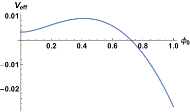
Figure 2: Plot of the effective potential for the inverted quadratic case for $\kappa=1$, $m_{\psi}=0.1$, $a=0.25=1/\mu$, and $\lambda=1.0$. As given below (42), $C=0.643$.

IV Dynamics

The effective potential is not suitable for describing the evolution of the background because the derivation assumes that the quantum field $\psi$ is in its vacuum. In the dynamical problem, as the field $\phi$ rolls, quanta of $\psi$ are excited and the field $\psi$ is no longer in its vacuum. The production of $\psi$ quanta backreacts on the dynamics of $\phi$. We shall now solve this dynamical problem, separately considering homogeneous and inhomogeneous backgrounds.

IV.1 Dynamics with homogeneity

The first question we ask is if the initial conditions for $\phi$ are homogeneous, can the dynamics make $\phi$ inhomogeneous? As this is a dynamical question, we use the CQC equations in (13) and (14) and check that homogeneous evolution is self-consistent.

For homogeneous $\phi$, Eq. (12) can be written in a more convenient way as

$$\Omega^{2}_{ij}=-\nabla^{2}_{ij}+M^{2}\delta_{ij}$$ (49)

where $M^{2}=m^{2}+\lambda\phi^{2}$ and the Laplacian matrix is given by,

$$a^{2}\nabla^{2}_{ij}=\delta_{i+1,j}-2\delta_{ij}+\delta_{i-1,j}$$ (50)

where the indices are integers mod $N$. The $\nabla^{2}$ has translational symmetry, i.e.

$$\nabla^{2}_{ij}=\nabla^{2}_{i+s,j+s}$$ (51)

where $s$ is any integer. Alternately, $\nabla^{2}_{ij}$ only depends on the difference $i-j$ (mod $N$). Then $\Omega^{2}_{ij}$ is also translationally invariant and only depends on the difference $i-j$

$$\Omega^{2}_{i+s,j+s}=\Omega^{2}_{i,j}$$ (52)

In particular, this implies $\Omega^{2}_{nn}$ is independent of $n$, as already discussed below (31).

Using Eqs. (24), (25) and (26) we can check that the initial conditions for $Z_{ij}$ are also translationally invariant,

$$Z_{0;i+s,j+s}=Z_{0;i,j},\ \ {\dot{Z}}_{0;i+s,j+s}={\dot{Z}}_{0;i,j}$$ (53)

when $\phi$ is homogeneous.

Next we consider the equation for $Z_{n+s,j+s}$ in (13).

$$0 = {\ddot{Z}}_{n+s,j+s}+\sum_{k=1}^{N}\Omega^{2}_{n+s,k}\,Z_{k,j+s}$$ (54)

$$= {\ddot{Z}}_{n+s,j+s}+\sum_{l=1}^{N}\Omega^{2}_{n+s,l+s}\,Z_{l+s,j+s}$$

$$= {\ddot{Z}}_{n+s,j+s}+\sum_{l=1}^{N}\Omega^{2}_{n,l}\,Z_{l+s,j+s}$$

In the above derivation we have changed the summation index from $k$ to $l+s$ in the second line and used (52) in the third line. Now subtracting (13) gives

$$({\ddot{Z}}_{n+s,j+s}-{\ddot{Z}}_{n,j})+\sum_{l=1}^{N}\Omega^{2}_{n,l}(Z_{l+s,j+s}-Z_{l,j})=0$$ (55)

With the initial conditions in (53), the solution is

$$Z_{n+s,j+s}(t)=Z_{n,j}(t)$$ (56)

i.e. $Z_{n,j}$ is invariant under translations while $\phi$ is homogeneous.

Making use of the translational symmetry, we can write $Z_{nj}=a\chi_{n-j}$. Then going back to the equation for $\phi$ in (14), we see

$$\frac{1}{a^{2}}\sum_{j=1}^{N}Z_{nj}^{*}Z_{nj}=\sum_{j=1}^{N}\chi_{n-j}^{*}\chi_{n-j}\\ =\sum_{k=1}^{N}\chi_{k}^{*}\chi_{k}$$

which is independent of $n$. Thus the $\phi_{n}$ equation is independent of $n$ and the evolution of $\phi$ is homogeneous. Thus homogeneous initial conditions will lead to homogeneous evolution.

IV.2 CQC for fields with homogeneous background

The result above, that translational symmetry of the background is preserved on evolution, suggests that the system of CQC equations simplify when the background is homogeneous. Indeed we will show here that translational symmetry of the background implies that our quantum system corresponds to a classical field theory. Whereas the quantum system has the real scalar fields $\phi$ and $\psi$, the classical system has the background $\phi$ and a complex scalar field $\chi$ that is to be evolved with specific initial conditions.

For homogeneous backgrounds we have already introduced $\chi_{n-j}=Z_{nj}/a$ above (IV.1). Then the $\phi$ equation becomes

$${\ddot{\phi}}+V^{\prime}(\phi)+\lambda\left(\sum_{j=1}^{N}\chi_{j}^{*}\chi_{j}\right)\phi=0$$ (57)

where we have written $\phi_{n}$ as $\phi$ since it is homogeneous. Similarly, after some manipulation, (13) with (49) leads to

$${\ddot{\chi}}_{n}-\frac{1}{a^{2}}(\chi_{n+1}-2\chi_{n}+\chi_{n-1})+M^{2}\chi_{n}=0$$ (58)

which is the discretized version of

$$\square\chi+M^{2}\chi=0$$ (59)

where $\square$ is the D’Alembertian operator and note that $\chi$ is complex. Hence the original system where we had a classical field $\phi$ and a quantum field $\psi$ has been transformed into a system with $\phi$ and a classical complex field $\chi$.

We would now like to solve the system of equations in (57) and (58) with initial conditions following from those specified in Sec. II,

$$\chi_{q}(t=0)=\frac{-i}{\sqrt{2a}N}\sum_{k=1}^{N}\frac{e^{-ikq2\pi/N}}{\left[\frac{4}{a^{2}}\sin^{2}\left(\frac{\pi k}{N}\right)+M_{0}^{2}\right]^{1/4}}$$ (60)

$${\dot{\chi}}_{q}(t=0) = \frac{1}{\sqrt{2a}N}\sum_{k=1}^{N}\left[\frac{4}{a^{2}}\sin^{2}\left(\frac{\pi k}{N}\right)+M_{0}^{2}\right]^{1/4}$$ (61)

$$\hskip 71.13188pt\times e^{-ikq2\pi/N}$$

where $M_{0}^{2}=m^{2}+\lambda\phi(t=0)^{2}$.

We can simplify the equations further by performing a discrete Fourier transform,

$$\chi_{n}=\frac{1}{\sqrt{N}}\sum_{k}c_{k}(t)e^{-ink2\pi/N}$$ (62)

Then the equation for the mode coefficients $c_{k}$ are ordinary differential equations

$${\ddot{c}}_{k}+\left[\frac{4}{a^{2}}\sin^{2}\left(\frac{\pi k}{N}\right)+M^{2}\right]c_{k}=0$$ (63)

with the initial conditions

$$c_{k}(t=0)=\frac{-i}{\sqrt{2aN}}\left[\frac{4}{a^{2}}\sin^{2}\left(\frac{\pi k}{N}\right)+M_{0}^{2}\right]^{-1/4}$$ (64)

$${\dot{c}}_{k}(t=0)=\frac{1}{\sqrt{2aN}}\left[\frac{4}{a^{2}}\sin^{2}\left(\frac{\pi k}{N}\right)+M_{0}^{2}\right]^{1/4}$$ (65)

Further reduction in the number of variables can be obtained at the cost of introducing some non-linearity by letting

$$c_{k}=\rho_{k}e^{i\theta_{k}}$$ (66)

Then angular momentum ($\rho_{k}^{2}{\dot{\theta}}_{k}$) conservation together with the initial conditions gives

$${\dot{\theta}}_{k}=\frac{1}{2L\rho_{k}^{2}}$$ (67)

and the equation for $\rho_{k}$ is

$${\ddot{\rho}}_{k}+\left[\frac{4}{a^{2}}\sin^{2}\left(\frac{\pi k}{N}\right)+M^{2}\right]\rho_{k}=\frac{1}{4L^{2}\rho_{k}^{3}}$$ (68)

with initial conditions

$$\rho_{k}(0) = \frac{1}{\sqrt{2L}}\left[\frac{4}{a^{2}}\sin^{2}\left(\frac{\pi k}{N}\right)+M_{0}^{2}\right]^{-1/4},$$ (69)

$${\dot{\rho}}_{k}(0) = 0.$$ (70)

Advantage can also be taken of the symmetry $k\to N-k$ and then we only need to solve for $N/2+1$ of the $\rho_{k}$’s.

In terms of the $\rho_{k}$’s, the equation for $\phi$ is,

$${\ddot{\phi}}+V^{\prime}(\phi)+\lambda\sum_{k=1}^{N}\rho_{k}^{2}\,\phi=0$$ (71)

To summarize our results in this section, a quantum real scalar field in a homogeneous time-dependent (“rolling”) background field is equivalent to a classical complex scalar field in the same background with specific interactions with the background and specific initial conditions. In the discretized version, the quantum rolling problem is thus equivalent to $2N+1$ (recall that $c_{k}$’s are complex) second order ordinary differential equations (63), (71) with the initial conditions (64), (65) and chosen initial conditions for homogeneous $\phi$. The problem can be reduced to $(N/2+1)+1$ second order ordinary differential equations by going to the real $\rho_{k}$ variables and using the $k\to N-k$ symmetry.

IV.3 Dynamics in a linear potential

Figure 3: Plot of $\phi$ versus time for $\lambda=0.3$ (black), 0.4 (red), 0.5 (dark purple), 0.6 (light purple), 0.7 (dark green), 0.8 (light green), 0.9 (orange) and 1.0 (blue), and other parameters as given in the text.

Figure 4: Plot of $\phi$ versus time for $\lambda=0.3$ using the effective potential. This is to be contrasted with the CQC solution for $\lambda=0.3$, shown as the black curve in Fig. 3.

For the particular case of a linear potential, we have solved for the evolution of $\phi$ using the CQC equations in Sec. II with the potential in (38) ($K=-1$) and the $\phi$ initial conditions $\phi_{n}(0)=0={\dot{\phi}}_{n}(0)$. The solutions for $\phi(t)$ for several different values of $\lambda$ and with parameters $a=0.25$, $N=400$, $L=100$, $m=0.1$, are shown in Fig. 3.

The plots show that $\phi$ does not increase monotonically as we might expect based on rolling on a classical linear potential; instead $\phi$ oscillates, as one might expect based on the effective potential analysis. To compare the CQC dynamics with that of rolling on the effective potential, we have solved the “effective equation of motion”,

$${\ddot{\phi}}+V_{\rm eff}^{\prime}(\phi)=0$$ (72)

where $V_{\rm eff}(\phi)$ is given in (36) and $V(\phi)=-\phi$. Fig. 4 shows the rolling solution on the effective potential for $\lambda=0.3$. It is to be compared to the corresponding curve in Fig. 3.

A few features of the dynamics stand out: the field $\phi$ oscillates in the full dynamics (Fig. 3) but at a much smaller frequency than in the effective potential treatment (Fig. 4); the amplitude of oscillations in the effective potential stays constant and is much smaller than in the CQC. This is surprising since the physical argument is that $\psi$ particles are produced during rolling and this is what causes differences between the full dynamics and the dynamics on the effective potential. However, increased particle production might be expected to increase $\langle\psi^{2}\rangle$ and this should cause the $\phi$ oscillations in the full dynamics to have smaller amplitude than in the effective potential. The resolution is that even though there is particle production, $\langle\psi^{2}\rangle$ actually decreases as is evident in Fig. 5. This can happen if most of the energy in particle production goes into the kinetic energy and not in $\langle\psi^{2}\rangle$. Then with a smaller $\langle\psi^{2}\rangle$ we do expect the $\phi$ oscillations to have larger amplitude in the full dynamics.

Figure 5: Plot of $\langle\psi^{2}\rangle$ versus time for $\lambda=0.3$.

In the CQC solution, let us denote the first maximum value of $\phi$ by $\phi_{\rm max}$ and the time at which this value is reached by $t_{\rm max}$. In Fig. 6 we show $\phi_{\rm max}$ as a function of $\lambda$ on a log-log plot. It is clear that the data is not fit by a power law as the fit varies from $\phi_{\rm max}\sim\lambda^{-3.2}$ for smaller $\lambda$ to $\phi_{\rm max}\sim\lambda^{-1.7}$ at larger $\lambda$. Fig. 7 shows $t_{\rm max}$ versus $\lambda$ on a log-log plot. Here too the fit varies from $t_{\rm max}\sim\lambda^{-1.9}$ to $\sim\lambda^{-0.9}$ at larger $\lambda$.

Figure 6: Log-log plot of the value of $\phi$ at the first turning point versus $\lambda$. The fit is not a straight line, ranging from $\phi_{\rm max}\sim\lambda^{-3.2}$ for smaller values of $\lambda$ and $\sim\lambda^{-1.7}$ for the larger values.

Figure 7: Log-log plot of the value of $t$ at the first turning point versus $\lambda$. The fit is not a straight line, ranging from $t_{\rm max}\sim\lambda^{-1.9}$ for smaller values of $\lambda$ and $\sim\lambda^{-0.9}$ for the larger values.

Even though we have shown that homogeneous initial conditions lead to homogeneous evolution, there remains the possibility that the evolution is unstable to developing inhomogeneities. We now address this question numerically by including small perturbations to homogeneous initial conditions.

IV.4 Dynamics with small initial inhomogeneities

To introduce inhomogeneous perturbations, we solve the CQC equations in (14), (13) but with the initial conditions

$$\phi_{n}(t=0)=0,\ \ {\dot{\phi}}_{n}(t=0)=\epsilon\sin\left(\frac{2\pi n\nu}{N}\right)$$ (73)

where $\epsilon$ is a small amplitude and the integer $\nu$ sets the wavenumber of the perturbation. The $Z$ initial conditions are still given by (15). The advantage of introducing the inhomogeneities in the time derivative ${\dot{\phi}}_{n}$ while keeping $\phi_{n}$ homogeneous is that then we can continue to use (24) with the formula for $O$ and $D$ given in Sec. III.1.

We now write the field $\phi$ as

$$\phi={\bar{\phi}}+{\delta\phi}$$ (74)

where the homogeneous part is

$${\bar{\phi}}(t)\equiv\frac{1}{N}\sum_{n=1}^{N}\phi_{n}$$ (75)

The energy in the inhomogeneous part is

$$E_{\rm inhom}=a\sum_{n=1}^{N}\left[\frac{1}{2}({\delta{\dot{\phi}}}_{n})^{2}+\frac{1}{2}\left(\frac{{\delta\phi}_{n+1}-{\delta\phi}_{n-1}}{2a}\right)^{2}\right]$$ (76)

In Fig. 8 we show $E_{\rm inhom}$ versus $t$ for $\lambda=1.0$, $\epsilon=0.1$ and $\nu=N/10$. It is clear that the energy in the inhomogeneities decreases with time, though with some fluctuations, and there is no instability in the system. We find similar evolution for other values of $\nu$.

Figure 8: Energy in inhomogeneity versus time for $\lambda=1.0$ $\epsilon=0.1$ and $\nu=N/10$.

V Conclusions

We have solved for the dynamics of a classical rolling field that is coupled to a quantum field using the CQC.

Static solutions of the CQC equations are simply the extrema of the effective potential. For the particular model in (1) with the linear potential of (38), the effective potential has a minimum in the regime of validity of our equations only if the interaction strength is stronger than a critical value as in (42). For weaker interactions, there may be a minimum but it would lie beyond our cutoff.

The CQC equations are then used to study the dynamics of rolling on the linear potential. With homogeneous initial conditions, we find that the background field oscillates. This is similar to what we would expect from the effective potential picture but there are sharp differences in the details. These are most easily seen in Figs. 3 and 4 and are understood by noting that the CQC solves for the full dynamics, including particle production and backreaction, whereas the effective potential picture is limited to static backgrounds.

In order to study possible dynamical instabilities, we have also examined the case when the background field is weakly inhomogeneous. Our numerical results show that small inhomogeneities in the initial conditions diminish on evolution and there is no indication of an instability.

Our analysis is directly relevant to phase transitions in which the order parameter acquires a vacuum expectation value. The CQC equations can be used to study the dynamics of phase transitions, in particular the formation of topological defects. However, it would become necessary to generalize the CQC to the case when the quantum field has self-interactions. One way to deal with self-interactions, e.g. a $\psi^{4}$ term in the action, is to use perturbation theory on top of the CQC solution. That is, the solution to the CQC equations would serve as the zeroth order solution around which self-interactions could be treated perturbatively. This scheme has not yet been implemented.

Our result that homogeneous initial conditions evolve homogeneously is equivalent to saying that the quantum dynamics does not spontaneously break translational invariance. This is in contrast to the claim that cosmological inflation due to a rolling homogeneous field produces density fluctuations and thus spontaneously breaks translational symmetry Mukhanov and Chibisov (1981). However, further investigation of this issue is necessary because there are additional ingredients that go into the inflationary calculation. In particular, quantum fluctuations convert into classical fluctuations once they exit the cosmological horizon Kiefer et al. (1998), and cosmological expansion provides dissipation. It will be interesting to capture these effects in the CQC formulation.