DeepXDE: A deep learning library for solving differential equations

Abstract

Deep learning has achieved remarkable success in diverse applications; however, its use in solving partial differential equations (PDEs) has emerged only recently. Here, we present an overview of physics-informed neural networks (PINNs), which embed a PDE into the loss of the neural network using automatic differentiation. The PINN algorithm is simple, and it can be applied to different types of PDEs, including integro-differential equations, fractional PDEs, and stochastic PDEs. Moreover, from the implementation point of view, PINNs solve inverse problems as easily as forward problems. We propose a new residual-based adaptive refinement (RAR) method to improve the training efficiency of PINNs. For pedagogical reasons, we compare the PINN algorithm to a standard finite element method. We also present a Python library for PINNs, DeepXDE, which is designed to serve both as an education tool to be used in the classroom as well as a research tool for solving problems in computational science and engineering. Specifically, DeepXDE can solve forward problems given initial and boundary conditions, as well as inverse problems given some extra measurements. DeepXDE supports complex-geometry domains based on the technique of constructive solid geometry, and enables the user code to be compact, resembling closely the mathematical formulation. We introduce the usage of DeepXDE and its customizability, and we also demonstrate the capability of PINNs and the user-friendliness of DeepXDE for five different examples. More broadly, DeepXDE contributes to the more rapid development of the emerging Scientific Machine Learning field.

65-01, 65-04, 65L99, 65M99, 65N99

1 Introduction

In the last 15 years, deep learning in the form of deep neural networks (NNs), has been used very effectively in diverse applications [32], such as computer vision and natural language processing. Despite the remarkable success in these and related areas, deep learning has not yet been widely used in the field of scientific computing. However, more recently, solving partial differential equations (PDEs), e.g., in the standard differential form or in the integral form, via deep learning has emerged as a potentially new sub-field under the name of Scientific Machine Learning (SciML) [4]. In particular, we can replace traditional numerical discretization methods with a neural network that approximates the solution to a PDE.

To obtain the approximate solution of a PDE via deep learning, a key step is to constrain the neural network to minimize the PDE residual, and several approaches have been proposed to accomplish this. Compared to the traditional mesh-based methods, such as the finite difference method (FDM) and the finite element method (FEM), deep learning could be a mesh-free approach by taking advantage of the automatic differentiation [47], and could break the curse of dimensionality [45, 18]. Among these approaches, some can only be applied to particular types of problems, such as image-like input domain [28, 33, 58] or parabolic PDEs [6, 19]. Some researchers adopt the variational form of PDEs and minimize the corresponding energy functional [16, 20]. However, not all PDEs can be derived from a known functional, and thus Galerkin type projections have also been considered [39]. Alternatively, one could use the PDE in strong form directly [15, 52, 30, 31, 7, 50, 47]; in this form, automatic differentiation could be used directly to avoid truncation errors and the numerical quadrature errors of variational forms. This strong form approach was introduced in [47] coining the term physics-informed neural networks (PINNs). An attractive feature of PINNs is that it can be used to solve inverse problems with minimum change of the code for forward problems [47, 48, 51, 21, 13]. In addition, PINNs have been further extended to solve integro-differential equations (IDEs), fractional differential equations (FDEs) [42], and stochastic differential equations (SDEs) [57, 55, 41, 56].

In this paper, we present various PINN algorithms implemented in a Python library DeepXDE, which is designed to serve both as an education tool to be used in the classroom as well as a research tool for solving problems in computational science and engineering (CSE). DeepXDE can be used to solve multi-physics problems, and supports complex-geometry domains based on the technique of constructive solid geometry (CSG), hence avoiding tedious and time-consuming computational geometry tasks. By using DeepXDE, time-dependent PDEs can be solved as easily as steady states by only defining the initial conditions. In addition to the main workflow of DeepXDE, users can readily monitor and modify the solution process via callback functions, e.g., monitoring the Fourier spectrum of the neural network solution, which can reveal the learning mode of the NN Fig. 2. Last but not least, DeepXDE is designed to make the user code stay compact and manageable, resembling closely the mathematical formulation.

The paper is organized as follows. In Section 2, after briefly introducing deep neural networks and automatic differentiation, we present the algorithm, approximation theory, and error analysis of PINNs, and make a comparison between PINNs and FEM. We then discuss how to use PINNs to solve integro-differential equations and inverse problems. In addition, we propose the residual-based adaptive refinement (RAR) method to improve the training efficiency of PINNs. In Section 3, we introduce the usage of our library, DeepXDE, and its customizability. In Section 4, we demonstrate the capability of PINNs and friendly use of DeepXDE for five different examples. Finally, we conclude the paper in Section 5.

2 Algorithm and theory of physics-informed neural networks

In this section, we first provide a brief overview of deep neural networks and automatic differentiation, and present the algorithm and theory of PINNs for solving PDEs. We then make a comparison between PINNs and FEM, and discuss how to use PINNs to solve integro-differential equations and inverse problems. Next we propose RAR, an efficient way to select the residual points adaptively during the training process.

2.1 Deep neural networks

Mathematically, a deep neural network is a particular choice of a compositional function. The simplest neural network is the feed-forward neural network (FNN), also called multilayer perceptron (MLP), which applies linear and nonlinear transformations to the inputs recursively. Although many different types of neural networks have been developed in the past decades, such as the convolutional neural network and the recurrent neural network. In this paper we consider FNN, which is sufficient for most PDE problems, and residual neural network (ResNet), which is easier to train for deep networks. However, it is straightforward to employ other types of neural networks.

Let $\mathcal{N}^{L}(\mathbf{x}):\mathbb{R}^{d_{\text{in}}}\to\mathbb{R}^{d_{\text{out}}}$ be a $L$-layer neural network, or a $(L-1)$-hidden layer neural network, with $N_{\ell}$ neurons in the $\ell$-th layer ($N_{0}=d_{\text{in}}$, $N_{L}=d_{\text{out}}$). Let us denote the weight matrix and bias vector in the $\ell$-th layer by $\bm{W}^{\ell}\in\mathbb{R}^{N_{\ell}\times N_{\ell-1}}$ and $\mathbf{b}^{\ell}\in\mathbb{R}^{N_{\ell}}$, respectively. Given a nonlinear activation function $\sigma$, which is applied element-wisely, the FNN is recursively defined as follows:

input layer: $$\quad\mathcal{N}^{0}(\textbf{x})=\textbf{x}\in\mathbb{R}^{d_{\text{in}}},$$

hidden layers: $$\quad\mathcal{N}^{\ell}(\textbf{x})=\sigma(\bm{W}^{\ell}\mathcal{N}^{\ell-1}(\textbf{x})+\bm{b}^{\ell})\in\mathbb{R}^{N_{\ell}},\quad\text{for}\quad 1\leq\ell\leq L-1,$$

output layer: $$\quad\mathcal{N}^{L}(\textbf{x})=\bm{W}^{L}\mathcal{N}^{L-1}(\textbf{x})+\bm{b}^{L}\in\mathbb{R}^{d_{\text{out}}};$$

see also a visualization of a neural network in Fig. 1. Commonly used activation functions include the logistic sigmoid $1/(1+e^{-x})$, the hyperbolic tangent ($\tanh$), and the rectified linear unit (ReLU, $\max\{x,0\}$).

2.2 Automatic differentiation

In PINNs, it is required to compute the derivatives of the network outputs with respect to the network inputs. There are four possible methods for computing the derivatives [5, 38]: (1) hand-coded analytical derivative; (2) finite difference or other numerical approximations; (3) symbolic differentiation (used in software programs such as Mathematica, Maxima, and Maple); and (4) automatic differentiation (AD, also called algorithmic differentiation). In deep learning, the derivatives are evaluated using backpropagation [49], a specialized technique of AD.

Considering the fact that the neural network represents a compositional function, then AD applies the chain rule repeatedly to compute the derivatives. There are two steps in AD: one forward pass to compute the values of all variables, and one backward pass to compute the derivatives. To demonstrate AD, we consider a FNN of only one hidden layer with two inputs $x_{1}$ and $x_{2}$ and one output $y$:

$$v =-2x_{1}+3x_{2}+0.5,$$

$$h =\tanh v,$$

$$y =2h-1.$$

The forward pass and backward pass of AD for computing the partial derivatives $\frac{\partial y}{\partial x_{1}}$ and $\frac{\partial y}{\partial x_{2}}$ at $(x_{1},x_{2})=(2,1)$ are shown in Table 1.

We can see that AD only requires one forward pass and one backward pass to compute all the partial derivatives, no matter what the input dimension is. In contrast, using finite differences computing each partial derivative $\frac{\partial y}{\partial x_{i}}$ requires two function valuations $y(x_{1},\dots,x_{i},\dots,x_{d_{\text{in}}})$ and $y(x_{1},\dots,x_{i}+\Delta x_{i},\dots,x_{d_{\text{in}}})$ for some small number $\Delta x_{i}$, and thus in total $d_{\text{in}}+1$ forward passes are required to evaluate all the partial derivatives. Hence, AD is much more efficient than finite difference when the input dimension is high (see [5, 38] for more details of the comparison between AD and the other three methods). To compute $n^{th}$-order derivatives, AD can be applied recursively $n$ times. However, this nested approach may lead to inefficiency and numerical instability, and hence other methods, e.g., Taylor-Mode AD, have been developed for this purpose [8, 9]. Finally we note that with AD we differentiate the NN and therefore we can deal with noisy data [42].

Table 1: Example of AD to compute the partial derivatives $\frac{\partial y}{\partial x_{1}}$ and $\frac{\partial y}{\partial x_{2}}$ at $(x_{1},x_{2})=(2,1)$.

Forward pass	Backward pass
$x_{1}=2$	$\frac{\partial y}{\partial y}=1$
$x_{2}=1$
$v=-2x_{1}+3x_{2}+0.5=-0.5$	$\frac{\partial y}{\partial h}=\frac{\partial(2h-1)}{\partial h}=2$
$h=\tanh v\approx-0.462$	$\frac{\partial y}{\partial v}=\frac{\partial y}{\partial h}\frac{\partial h}{\partial v}=\frac{\partial y}{\partial h}\text{sech}^{2}(v)\approx 1.573$
$y=2h-1=-1.924$	$\frac{\partial y}{\partial x_{1}}=\frac{\partial y}{\partial v}\frac{\partial v}{\partial x_{1}}=\frac{\partial y}{\partial v}\times(-2)=-3.146$
	$\frac{\partial y}{\partial x_{2}}=\frac{\partial y}{\partial v}\frac{\partial v}{\partial x_{2}}=\frac{\partial y}{\partial v}\times 3=4.719$

2.3 Physics-informed neural networks (PINNs) for solving PDEs

We consider the following PDE parameterized by $\bm{\lambda}$ for the solution $u(\mathbf{x})$ with $\mathbf{x}=(x_{1},\dots,x_{d})$ defined on a domain $\Omega\subset\mathbb{R}^{d}$:

(1) $$f\left(\mathbf{x};\frac{\partial u}{\partial x_{1}},\dots,\frac{\partial u}{\partial x_{d}};\frac{\partial^{2}u}{\partial x_{1}\partial x_{1}},\dots,\frac{\partial^{2}u}{\partial x_{1}\partial x_{d}};\dots;\bm{\lambda}\right)=0,\quad\mathbf{x}\in\Omega,$$

with suitable boundary conditions

$$\mathcal{B}(u,\mathbf{x})=0\quad\text{on}\quad\partial\Omega,$$

where $\mathcal{B}(u,\mathbf{x})$ could be Dirichlet, Neumann, Robin, or periodic boundary conditions. For time-dependent problems, we consider time $t$ as a special component of $\mathbf{x}$, and $\Omega$ contains the temporal domain. The initial condition can be simply treated as a special type of Dirichlet boundary condition on the spatio-temporal domain.

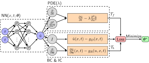
Figure 1: Schematic of a PINN for solving the diffusion equation $\frac{\partial u}{\partial t}=\lambda\frac{\partial^{2}u}{\partial x^{2}}$ with mixed boundary conditions (BC) $u(x,t)=g_{D}(x,t)$ on $\Gamma_{D}\subset\partial\Omega$ and $\frac{\partial u}{\partial\mathbf{n}}(x,t)=g_{R}(u,x,t)$ on $\Gamma_{R}\subset\partial\Omega$. The initial condition (IC) is treated as a special type of boundary conditions. $\mathcal{T}_{f}$ and $\mathcal{T}_{b}$ denote the two sets of residual points for the equation and BC/IC.

Procedure 1 The PINN algorithm for solving differential equations.

1. Construct a neural network $\hat{u}(\mathbf{x};\bm{\theta})$ with parameters $\bm{\theta}$.

2. Specify the two training sets $\mathcal{T}_{f}$ and $\mathcal{T}_{b}$ for the equation and boundary/initial conditions.

3. Specify a loss function by summing the weighted $L^{2}$ norm of both the PDE equation and boundary condition residuals.

4. Train the neural network to find the best parameters $\bm{\theta}^{*}$ by minimizing the loss function $\mathcal{L}(\bm{\theta};\mathcal{T}).$

The algorithm of PINN [31, 47] is shown in Procedure 1, and visually in the schematic of Fig. 1 solving a diffusion equation $\frac{\partial u}{\partial t}=\lambda\frac{\partial^{2}u}{\partial x^{2}}$ with mixed boundary conditions $u(x,t)=g_{D}(x,t)$ on $\Gamma_{D}\subset\partial\Omega$ and $\frac{\partial u}{\partial\mathbf{n}}(x,t)=g_{R}(u,x,t)$ on $\Gamma_{R}\subset\partial\Omega$. We explain each step as follows. In a PINN, we first construct a neural network $\hat{u}(\mathbf{x};\bm{\theta})$ as a surrogate of the solution $u(\mathbf{x})$, which takes the input $\mathbf{x}$ and outputs a vector with the same dimension as $u$. Here, $\bm{\theta}=\{\bm{W}^{\ell},\bm{b}^{\ell}\}_{1\leq\ell\leq L}$ is the set of all weight matrices and bias vectors in the neural network $\hat{u}$. One advantage of PINNs by choosing neural networks as the surrogate of $u$ is that we can take the derivatives of $\hat{u}$ with respect to its input $\mathbf{x}$ by applying the chain rule for differentiating compositions of functions using the automatic differentiation (AD), which is conveniently integrated in machine learning packages, such as TensorFlow [1] and PyTorch [43].

In the next step, we need to restrict the neural network $\hat{u}$ to satisfy the physics imposed by the PDE and boundary conditions. In practice, we restrict $\hat{u}$ on some scattered points (e.g., randomly distributed points, or clustered points in the domain [37]), i.e., the training data $\mathcal{T}=\{\mathbf{x}_{1},\mathbf{x}_{2},\dots,\mathbf{x}_{|\mathcal{T}|}\}$ of size $|\mathcal{T}|$. In addition, $\mathcal{T}$ is comprised of two sets $\mathcal{T}_{f}\subset\Omega$ and $\mathcal{T}_{b}\subset\partial\Omega$, which are the points in the domain and on the boundary, respectively. We refer $\mathcal{T}_{f}$ and $\mathcal{T}_{b}$ as the sets of “residual points”.

To measure the discrepancy between the neural network $\hat{u}$ and the constraints, we consider the loss function defined as the weighted summation of the $L^{2}$ norm of residuals for the equation and boundary conditions:

(2) $$\mathcal{L}(\bm{\theta};\mathcal{T})=w_{f}\mathcal{L}_{f}(\bm{\theta};\mathcal{T}_{f})+w_{b}\mathcal{L}_{b}(\bm{\theta};\mathcal{T}_{b}),$$

where

$$\mathcal{L}_{f}(\bm{\theta};\mathcal{T}_{f}) =\frac{1}{|\mathcal{T}_{f}|}\sum_{\mathbf{x}\in\mathcal{T}_{f}}\left\|f\left(\mathbf{x};\frac{\partial\hat{u}}{\partial x_{1}},\dots,\frac{\partial\hat{u}}{\partial x_{d}};\frac{\partial^{2}\hat{u}}{\partial x_{1}\partial x_{1}},\dots,\frac{\partial^{2}\hat{u}}{\partial x_{1}\partial x_{d}};\dots;\bm{\lambda}\right)\right\|_{2}^{2},$$

$$\mathcal{L}_{b}(\bm{\theta};\mathcal{T}_{b}) =\frac{1}{|\mathcal{T}_{b}|}\sum_{\mathbf{x}\in\mathcal{T}_{b}}\|\mathcal{B}(\hat{u},\mathbf{x})\|_{2}^{2},$$

and $w_{f}$ and $w_{b}$ are the weights. The loss involves derivatives, such as the partial derivative $\partial\hat{u}/\partial x_{1}$ or the normal derivative at the boundary $\partial\hat{u}/\partial\mathbf{n}=\nabla\hat{u}\cdot\mathbf{n}$, which are handled via AD.

In the last step, the procedure of searching for a good $\bm{\theta}$ by minimizing the loss $\mathcal{L}(\bm{\theta};\mathcal{T})$ is called “training”. Considering the fact that the loss is highly nonlinear and non-convex with respect to $\bm{\theta}$ [10], we usually minimize the loss function by gradient-based optimizers, such as gradient descent, Adam [29], and L-BFGS [12]. We remark that based on our experience, for smooth PDE solutions L-BFGS can find a good solution with less iterations than Adam, because L-BFGS uses second-order derivatives of the loss function, while Adam only relies on first-order derivatives. However, for stiff solutions L-BFGS is more likely to be stuck at a bad local minimum. The required number of iterations highly depends on the problem (e.g., the smoothness of the solution), and to check whether the network converges or not, we can monitor the loss function or the PDE residual using callback functions. We also note that acceleration of training can be achieved by using adaptive activation function that may remove bad local minima, see [24, 23].

Unlike traditional numerical methods, for PINNs there is no guarantee of unique solutions, because PINN solutions are obtained by solving non-convex optimization problems, which in general do not have a unique solution. In practice, to achieve a good level of accuracy, we need to tune all the hyperparameters, e.g., network size, learning rate, and the number of residual points. The required network size depends highly on the smoothness of the PDE solution. For example, a small network (e.g., a few layers and twenty neurons per layer) is sufficient for solving the 1D Poisson equation, but a deeper and wider network is required for the 1D Burgers equation to achieve a similar level of accuracy. We also note that PINNs may converge to different solutions from different network initial values [42, 51, 21], and thus a common strategy is that we train PINNs from random initialization for a few times (e.g., 10 independent runs) and choose the network with the smallest training loss as the final solution.

In the algorithm of PINN introduced above, we enforce soft constraints of boundary/initial conditions through the loss $\mathcal{L}_{b}$. This approach can be used for complex domains and any type of boundary conditions. On the other hand, it is possible to enforce hard constraints for simple cases [30]. For example, when the boundary condition is $u(0)=u(1)=0$ with $\Omega=[0,1]$, we can simply choose the surrogate model as $\hat{u}(x)=x(x-1)\mathcal{N}(x)$ to satisfy the boundary condition automatically, where $\mathcal{N}(x)$ is a neural network.

We note that we have great flexibility in choosing the residual points $\mathcal{T}$, and here we provide three possible strategies:

1. We can specify the residual points at the beginning of training, which could be grid points on a lattice or random points, and never change them during the training process.

2. In each optimization iteration, we could select randomly different residual points.

3. We could improve the location of the residual points adaptively during training, e.g., the method proposed in Section 2.8.

When the number of residual points required is very large, e.g., in multiscale problems, it is computationally expensive to calculate the loss and gradient in every iteration. Instead of using all residual points, we can split the residual points into small batches, and in each iteration we only use one batch to calculate the loss and update model parameters; this is the so-called “mini-batch” gradient descent. The aforementioned strategy (2), i.e., re-sampling in each step, is a special case of mini-batch gradient descent by choosing $\mathcal{T}=\Omega$ with $|\mathcal{T}|=\infty$.

Recent studies show that for function approximation, neural networks learn target functions from low to high frequencies [46, 54], but here we show that the learning mode of PINNs is different due to the existence of high-order derivatives. For example, when we approximate the function $f(x)=\sum_{k=1}^{5}\sin(2kx)/(2k)$ in $[-\pi,\pi]$ by a NN, the function is learned from low to high frequency (Fig. 2A). However, when we employ a PINN to solve the Poisson equation $-f_{xx}=\sum_{k=1}^{5}2k\sin(2kx)$ with zero boundary conditions in the same domain, all frequencies are learned almost simultaneously (Fig. 2B). Interestingly, by comparing Fig. 2A and Fig. 2B we can see that at least in this case solving the PDE using a PINN is faster than approximating a function using a NN. We can monitor this training process using the callback functions in our library DeepXDE as discussed later.

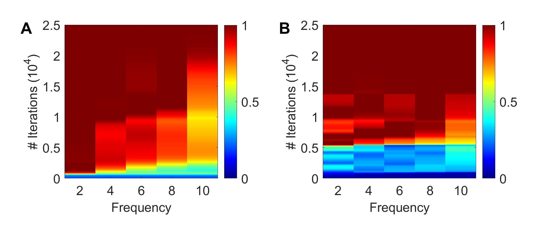
Figure 2: Convergence of the amplitude for each frequency during the training process. (A) A neural network is trained to approximate the function $f(x)=\sum_{k=1}^{5}\sin(2kx)/(2k)$. The color represents amplitude values with the maximum amplitude for each frequency normalized to 1. (B) A PINN is used to solve the Poisson equation $-f_{xx}=\sum_{k=1}^{5}2k\sin(2kx)$ with zero boundary conditions. We use a neural network of 4 hidden layers and 20 neurons per layer. The learning rate is chosen as $10^{-4}$, and 500 random points are sampled for training.

2.4 Approximation theory and error analysis for PINNs

One fundamental question related to PINNs is whether there exists a neural network satisfying both the PDE equation and the boundary conditions, i.e., whether there exists a neural network that can simultaneously and uniformly approximate a function and its partial derivatives. To address this question, we first introduce some notation. Let $\mathbb{Z}_{+}^{d}$ be the set of $d$-dimensional nonnegative integers. For $\mathbf{m}=(m_{1},\dots,m_{d})\in\mathbb{Z}_{+}^{d}$, we set $|\mathbf{m}|\coloneqq m_{1}+\dots+m_{d}$, and

$$D^{\mathbf{m}}\coloneqq\frac{\partial^{|\mathbf{m}|}}{\partial x_{1}^{m_{1}}\dots\partial x_{d}^{m_{d}}}.$$

We say $f\in C^{\mathbf{m}}(\mathbb{R}^{d})$ if $D^{\mathbf{k}}f\in C(\mathbb{R}^{d})$ for all $\mathbf{k}\leq\mathbf{m}$, $\mathbf{k}\in\mathbb{Z}_{+}^{d}$, where $C(\mathbb{R}^{d})=\{f:\mathbb{R}^{d}\to\mathbb{R}|f\text{ is continuous}\}$ is the space of continuous functions. Then, we recall the following theorem of derivative approximation using single hidden layer neural networks due to Pinkus [44].

Theorem 2.1.

Let $\mathbf{m}^{i}\in\mathbb{Z}_{+}^{d}$, $i=1,\dots,s$, and set $m=\max_{i=1,\dots,s}|\mathbf{m}^{i}|$. Assume $\sigma\in C^{m}(\mathbb{R})$ and $\sigma$ is not a polynomial. Then the space of single hidden layer neural nets

$$\mathcal{M}(\sigma)\coloneqq span\{\sigma(\mathbf{w}\cdot\mathbf{x}+b):\mathbf{w}\in\mathbb{R}^{d},b\in\mathbb{R}\}$$

is dense in

$$C^{\mathbf{m}^{1},\dots,\mathbf{m}^{s}}(\mathbb{R}^{d})\coloneqq\cap_{i=1}^{s}C^{\mathbf{m}^{i}}(\mathbb{R}^{d}),$$

i.e., for any $f\in C^{\mathbf{m}^{1},\dots,\mathbf{m}^{s}}(\mathbb{R}^{d})$, any compact $K\subset\mathbb{R}^{d}$, and any $\varepsilon>0$, there exists a $g\in\mathcal{M}(\sigma)$ satisfying

$$\max_{\mathbf{x}\in K}|D^{\mathbf{k}}f(\mathbf{x})-D^{\mathbf{k}}g(\mathbf{x})|<\varepsilon,$$

for all $\mathbf{k}\in\mathbb{Z}_{+}^{d}$ for which $\mathbf{k}\leq\mathbf{m}^{i}$ for some $i$.

Theorem 2.1 shows that feed-forward neural nets with enough neurons can simultaneously and uniformly approximate any function and its partial derivatives. However, neural networks in practice have limited size. Let $\mathcal{F}$ denote the family of all the functions that can be represented by our chosen neural network architecture. The solution $u$ is unlikely to belong to the family $\mathcal{F}$, and we define $u_{\mathcal{F}}=\arg\min_{f\in\mathcal{F}}\|f-u\|$ as the best function in $\mathcal{F}$ close to $u$ (Fig. 3). Because we only train the neural network on the training set $\mathcal{T}$, we define $u_{\mathcal{T}}=\arg\min_{f\in\mathcal{F}}\mathcal{L}(f;\mathcal{T})$ as the neural network whose loss is at global minimum. For simplicity, we assume that $u$, $u_{\mathcal{F}}$ and $u_{\mathcal{T}}$ are well defined and unique. Finding $u_{\mathcal{T}}$ by minimizing the loss is often computationally intractable [10], and our optimizer returns an approximate solution $\tilde{u}_{\mathcal{T}}$.

Figure 3: Illustration of errors of a PINN. The total error consists of the approximation error, the optimization error, and the generalization error. Here, $u$ is the PDE solution, $u_{\mathcal{F}}$ is the best function close to $u$ in the function space $\mathcal{F}$, $u_{\mathcal{T}}$ is the neural network whose loss is at a global minimum, and $\tilde{u}_{\mathcal{T}}$ is the function obtained by training a neural network.

We can then decompose the total error $\mathcal{E}$ as [11]

$$\mathcal{E}\coloneqq\|\tilde{u}_{\mathcal{T}}-u\|\leq\underbrace{\|\tilde{u}_{\mathcal{T}}-u_{\mathcal{T}}\|}_{\mathcal{E}_{\text{opt}}}+\underbrace{\|u_{\mathcal{T}}-u_{\mathcal{F}}\|}_{\mathcal{E}_{\text{gen}}}+\underbrace{\|u_{\mathcal{F}}-u\|}_{\mathcal{E}_{\text{app}}}.$$

The approximation error $\mathcal{E}_{\text{app}}$ measures how closely $u_{\mathcal{F}}$ can approximate $u$. The generalization error $\mathcal{E}_{\text{gen}}$ is determined by the number/locations of residual points in $\mathcal{T}$ and the capacity of the family $\mathcal{F}$. Neural networks of larger size have smaller approximation errors but could lead to higher generalization errors, which is called bias-variance tradeoff. Overfitting occurs when the generalization error dominates. In addition, the optimization error $\mathcal{E}_{\text{opt}}$ stems from the loss function complexity and the optimization setup, such as learning rate and number of iterations. However, currently there is no error estimation for PINNs yet, and even quantifying the three errors for supervised learning is still an open research problem [36, 35, 25].

2.5 Comparison between PINNs and FEM

To further explain the ideas of PINNs and to help those with the knowledge of FEM understand PINNs more easily, we make a comparison between PINNs and FEM point by point (Table 2):

• In FEM we approximate the solution $u$ by a piecewise polynomial with point values to be determined, while in PINNs we construct a neural network as the surrogate model parameterized by weights and biases.

• FEM typically requires a mesh generation, while PINN is totally mesh-free, and we can use either a grid or random points.

• FEM converts a PDE to an algebraic system, using the stiffness matrix and mass matrix, while PINN embeds the PDE and boundary conditions into the loss function.

• In the last step, the algebraic system in FEM is solved exactly by a linear solver, but the network in PINN is learned by a gradient-based optimizer.

At a more fundamental level, PINNs provide a nonlinear approximation to the function and its derivatives whereas FEM represent a linear approximation.

Table 2: Comparison between PINN and FEM.

	PINN	FEM
Basis function	Neural network (nonlinear)	Piecewise polynomial (linear)
Parameters	Weights and biases	Point values
Training points	Scattered points (mesh-free)	Mesh points
PDE embedding	Loss function	Algebraic system
Parameter solver	Gradient-based optimizer	Linear solver
Errors	$\mathcal{E}_{\text{app}}$, $\mathcal{E}_{\text{gen}}$ and $\mathcal{E}_{\text{opt}}$ (Section 2.4)	Approximation/quadrature errors
Error bounds	Not available yet	Partially available [14, 26]

2.6 PINNs for solving integro-differential equations

When solving integro-differential equations (IDEs), we still employ the automatic differentiation technique to analytically derive the integer-order derivatives, while we approximate integral operators numerically using classical methods (Fig. 4) [42], such as Gaussian quadrature. Therefore, we introduce a fourth error component, the discretization error $\mathcal{E}_{\text{dis}}$, due to the approximation of the integral by Gaussian quadrature.

For example, when solving

$$\frac{dy}{dx}+y(x)=\int_{0}^{x}e^{t-x}y(t)dt,$$

we first use Gaussian quadrature of degree $n$ to approximate the integral

$$\int_{0}^{x}e^{t-x}y(t)dt\approx\sum_{i=1}^{n}w_{i}e^{t_{i}(x)-x}y(t_{i}(x)),$$

and then we use a PINN to solve the following PDE instead of the original equation

$$\frac{dy}{dx}+y(x)\approx\sum_{i=1}^{n}w_{i}e^{t_{i}(x)-x}y(t_{i}(x)).$$

PINNs can also be easily extended to solve FDEs [42] and SDEs [57, 55, 41, 56], but we do not discuss here such cases due to the page limit.

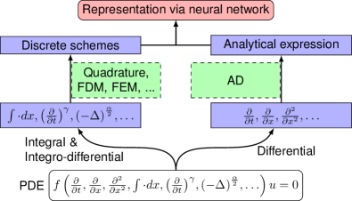
Figure 4: Schematic illustrating the modificaiton of the PINN algorithm for solving integro-differential equations. We employ the automatic differentiation technique to analytically derive the integer-order derivatives, and we approximate integral operators numerically using standard methods. (The figure is reproduced from [42].)

2.7 PINNs for solving inverse problems

In inverse problems, there are some unknown parameters $\bm{\lambda}$ in Eq. 1, but we have some extra information on some points $\mathcal{T}_{i}\subset\Omega$ besides the differential equation and boundary conditions:

$$\mathcal{I}(u,\mathbf{x})=0,\quad\text{for}\quad\mathbf{x}\in\mathcal{T}_{i}.$$

From the implementation point of view, PINNs solve inverse problems as easily as forward problems [47, 42]. The only difference between solving forward and inverse problems is that we add an extra loss term to Eq. 2:

$$\mathcal{L}(\bm{\theta},\bm{\lambda};\mathcal{T})=w_{f}\mathcal{L}_{f}(\bm{\theta},\bm{\lambda};\mathcal{T}_{f})+w_{b}\mathcal{L}_{b}(\bm{\theta},\bm{\lambda};\mathcal{T}_{b})+w_{i}\mathcal{L}_{i}(\bm{\theta},\bm{\lambda};\mathcal{T}_{i}),$$

where

$$\mathcal{L}_{i}(\bm{\theta},\bm{\lambda};\mathcal{T}_{i})=\frac{1}{|\mathcal{T}_{i}|}\sum_{\mathbf{x}\in\mathcal{T}_{i}}\|\mathcal{I}(\hat{u},\mathbf{x})\|_{2}^{2}.$$

We then optimize $\bm{\theta}$ and $\bm{\lambda}$ together, and our solution is $\bm{\theta}^{*},\bm{\lambda}^{*}=\arg\min_{\bm{\theta},\bm{\lambda}}\mathcal{L}(\bm{\theta},\bm{\lambda};\mathcal{T})$.

2.8 Residual-based adaptive refinement (RAR)

As we discussed in Section 2.3, the residual points $\mathcal{T}$ are usually randomly distributed in the domain. This works well for most cases, but it may not be efficient for certain PDEs that exhibit solutions with steep gradients. Take the Burgers equation as an example, intuitively we should put more points near the sharp front to capture the discontinuity well. However, it is challenging, in general, to design a good distribution of residual points for problems whose solution is unknown. To overcome this challenge, we propose a residual-based adaptive refinement (RAR) method to improve the distribution of residual points during training process (Procedure 2), conceptually similar to FEM refinement methods [2]. The idea of RAR is that we will add more residual points in the locations where the PDE residual $\left\|f\left(\mathbf{x};\frac{\partial\hat{u}}{\partial x_{1}},\dots,\frac{\partial\hat{u}}{\partial x_{d}};\frac{\partial^{2}\hat{u}}{\partial x_{1}\partial x_{1}},\dots,\frac{\partial^{2}\hat{u}}{\partial x_{1}\partial x_{d}};\dots;\bm{\lambda}\right)\right\|$ is large, and we repeat adding points until the mean residual

(3) $$\mathcal{E}_{r}=\frac{1}{V}\int_{\Omega}\left\|f\left(\mathbf{x};\frac{\partial\hat{u}}{\partial x_{1}},\dots,\frac{\partial\hat{u}}{\partial x_{d}};\frac{\partial^{2}\hat{u}}{\partial x_{1}\partial x_{1}},\dots,\frac{\partial^{2}\hat{u}}{\partial x_{1}\partial x_{d}};\dots;\bm{\lambda}\right)\right\|d\mathbf{x}$$

is smaller than a threshold $\mathcal{E}_{0}$, where $V$ is the volume of $\Omega$.

Procedure 2 RAR for improving the distribution of residual points for training.

1. Select the initial residual points $\mathcal{T}$, and train the neural network for a limited number of iterations.

2. Estimate the mean PDE residual $\mathcal{E}_{r}$ in Eq. 3 by Monte Carlo integration, i.e., by the average of values at a set of randomly sampled locations $\mathcal{S}=\{\mathbf{x}_{1},\mathbf{x}_{2},\dots,\mathbf{x}_{|\mathcal{S}|}\}$:

   $$\mathcal{E}_{r}\approx\frac{1}{|\mathcal{S}|}\sum_{\mathbf{x}\in\mathcal{S}}\left\|f\left(\mathbf{x};\frac{\partial\hat{u}}{\partial x_{1}},\dots,\frac{\partial\hat{u}}{\partial x_{d}};\frac{\partial^{2}\hat{u}}{\partial x_{1}\partial x_{1}},\dots,\frac{\partial^{2}\hat{u}}{\partial x_{1}\partial x_{d}};\dots;\bm{\lambda}\right)\right\|.$$

3. Stop if $\mathcal{E}_{r}<\mathcal{E}_{0}$. Otherwise, add $m$ new points with the largest residuals in $\mathcal{S}$ to $\mathcal{T}$, and go to Step 2.

3 DeepXDE usage and customization

In this section, we introduce the usage of DeepXDE and how to customize DeepXDE to meet new problem requirements.

3.1 Usage

Compared to traditional numerical methods, the code written with DeepXDE is much shorter and more comprehensive, resembling closely the mathematical formulation. Solving differential equations in DeepXDE is no more than specifying the problem using the build-in modules, including computational domain (geometry and time), PDE equations, boundary/initial conditions, constraints, training data, neural network architecture, and training hyperparameters. The workflow is shown in Procedure 3 and Fig. 5.

Procedure 3 Usage of DeepXDE for solving differential equations.

1. Specify the computational domain using the geometry module.

2. Specify the PDE using the grammar of TensorFlow.

3. Specify the boundary and initial conditions.

4. Combine the geometry, PDE and boundary/initial conditions together into data.PDE or data.TimePDE for time-independent problems or for time-dependent problems, respectively. To specify training data, we can either set the specific point locations, or only set the number of points and then DeepXDE will sample the required number of points on a grid or randomly.

5. Construct a neural network using the maps module.

6. Define a Model by combining the PDE problem in Step 4 and the neural net in Step 5.

7. Call Model.compile to set the optimization hyperparameters, such as optimizer and learning rate. The weights in Eq. 2 can be set here by loss_weights.

8. Call Model.train to train the network from random initialization or a pre-trained model using the argument model_restore_path. It is extremely flexible to monitor and modify the training behavior using callbacks.

9. Call Model.predict to predict the PDE solution at different locations.

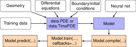
Figure 5: Flowchart of DeepXDE corresponding to Procedure 3. The white boxes define the PDE problem and the training hyperparameters. The blue boxes combine the PDE problem and training hyperparameters in the white boxes. The orange boxes are the three steps (from right to left) to solve the PDE.

In DeepXDE, the built-in primitive geometries include interval, triangle, rectangle, polygon, disk, cuboid and sphere. Other geometries can be constructed from these primitive geometries using three boolean operations: union (|), difference (-) and intersection (&). This technique is called constructive solid geometry (CSG), see Fig. 6 for examples. CSG supports both two-dimensional and three-dimensional geometries.

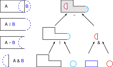
Figure 6: Examples of constructive solid geometry (CSG) in 2D. (left) A and B represent the rectangle and circle, respectively. The union $A|B$, difference $A-B$, and intersection $A\&B$ are constructed from A and B. (right) A complex geometry (top) is constructed from a polygon, a rectangle and two circles (bottom) through the union, difference, and intersection operations. This capability is included in the module geometry of DeepXDE.

DeepXDE supports four standard boundary conditions, including Dirichlet (DirichletBC), Neumann (NeumannBC), Robin (RobinBC), and periodic (PeriodicBC), and a more general BC can be defined using OperatorBC. The initial condition can be defined using IC. There are two types of neural networks available in DeepXDE: feed-forward neural network (maps.FNN) and residual neural network (maps.ResNet). It is also convenient to choose different training hyperparameters, such as loss types, metrics, optimizers, learning rate schedules, initializations and regularizations.

In addition to solving differential equations, DeepXDE can also be used to approximate functions from multi-fidelity data [40], and learn nonlinear operators [34].

3.2 Customizability

All the components of DeepXDE are loosely coupled, and thus DeepXDE is well-structured and highly configurable. In this subsection, we discuss how to customize DeepXDE to address new problem requirements, e.g., new geometry or network architecture.

3.2.1 Geometry

As we introduced above, DeepXDE has already supported 7 basic geometries and the CSG technique. However, it is still possible that the user needs a new geometry, which cannot be constructed in DeepXDE. In this situation, a new geometry can be defined as shown in Procedure 4. Currently DeepXDE does not support accurately descriptions of complex curvilinear boundaries; however, a future extension could be incorporation of the non-uniform rational basis spline (NURBS) [22] for such representations.

Procedure 4 Customization of the new geometry module MyGeometry. The class methods should only be implemented as needed.

⬇

class MyGeometry(Geometry):

def inside(self, x):

”””Check if x is inside the geometry.”””

def on_boundary(self, x):

”””Check if x is on the geometry boundary.”””

def boundary_normal(self, x):

”””Compute the unit normal at x for Neumann or Robin boundary conditions.”””

def periodic_point(self, x, component):

”””Compute the periodic image of x for periodic boundary condition.”””

def uniform_points(self, n, boundary=True):

”””Compute the equispaced point locations in the geometry.”””

def random_points(self, n, random=”pseudo”):

”””Compute the random point locations in the geometry.”””

def uniform_boundary_points(self, n):

”””Compute the equispaced point locations on the boundary.”””

def random_boundary_points(self, n, random=”pseudo”):

”””Compute the random point locations on the boundary.”””

3.2.2 Neural networks

DeepXDE currently supports two neural networks: feed-forward neural network (maps.FNN) and residual neural network (maps.ResNet). A new network can be added as shown in Procedure 5.

Procedure 5 Customization of the neural network MyNet.

⬇

class MyNet(Map):

@property

def inputs(self):

”””Return the net inputs.”””

@property

def outputs(self):

”””Return the net outputs.”””

@property

def targets(self):

”””Return the targets of the net outputs.”””

def build(self):

”””Construct the network.”””

3.2.3 Callbacks

It is usually a good strategy to monitor the training process of the neural network, and then make modifications in real time, e.g., change the learning rate. In DeepXDE, this can be implemented by adding a callback function, and here we only list a few commonly used ones already implemented in DeepXDE:

• ModelCheckpoint, which saves the model after certain epochs or when a better model is found.

• OperatorPredictor, which calculates the values of the operator applying on the outputs.

• FirstDerivative, which calculates the first derivative of the outpus with respect to the inputs. This is a special case of OperatorPredictor with the operator being the first derivative.

• MovieDumper, which dumps the movie of the function during the training progress, and/or the movie of the spectrum of its Fourier transform.

It is very convenient to add other callback functions, which will be called at different stages of the training process, see Procedure 6.

Procedure 6 Customization of the callback MyCallback. Here, we only show how to add functions to be called at the beginning/end of every epoch. Similarly, we can call functions at the other training stages, such as at the beginning of training.

⬇

class MyCallback(Callback):

def on_epoch_begin(self):

”””Called at the beginning of every epoch.”””

def on_epoch_end(self):

”””Called at the end of every epoch.”””

4 Demonstration examples

In this section, we use PINNs and DeepXDE to solve different problems. In all examples, we use the $\tanh$ as the activation function, and the other hyperparameters are listed in Table 3. The weights $w_{f}$, $w_{b}$ and $w_{i}$ in the loss function are set as 1. The codes of all examples are published in GitHub.

Table 3: Hyperparameters used for the following 5 examples. “Adam, L-BFGS” represents that we first use Adam for a certain number of iterations, and then switch to L-BFGS. The optimizer L-BFGS does not require learning rate, and the neural network is trained until convergence, so the number of iterations is also ignored for L-BFGS.

Example	NN Depth	NN Width	Optimizer	Learning rate	# Iterations
1	4	50	Adam, L-BFGS	0.001	50000
2	3	20	Adam, L-BFGS	0.001	15000
3	3	40	Adam	0.001	60000
4	3	20	Adam	0.001	80000
5	4	20	L-BFGS	-	-

4.1 Poisson equation over an L-shaped domain

Consider the following two-dimensional Poisson equation over an L-shaped domain $\Omega=[-1,1]^{2}\setminus[0,1]^{2}$:

$$-\Delta u(x,y) =1,\quad(x,y)\in\Omega,$$

$$u(x,y) =0,\quad(x,y)\in\partial\Omega.$$

We choose 1200 and 120 random points drawn from a uniform distribution as $\mathcal{T}_{f}$ and $\mathcal{T}_{b}$, respectively. The PINN solution is given in Fig. 7B. For comparison, we also present the numerical solution obtained by using the spectral element method (SEM) [27] (Fig. 7A). The result of the absolute error is shown in Fig. 7C.

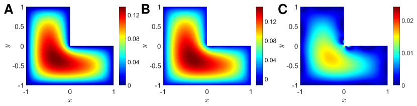
Figure 7: Example 4.1. Comparison of the PINN solution with the solution obtained by using spectral element method (SEM). (A) the SEM solution $u_{SEM}$, (B) the PINN solution $u_{NN}$, (C) the absolute error $|u_{SEM}-u_{NN}|$.

4.2 RAR for Burgers equation

We first consider the 1D Burgers equation:

$$\frac{\partial u}{\partial t}+u\frac{\partial u}{\partial x}=\nu\frac{\partial^{2}u}{\partial x^{2}},\quad x\in[-1,1],~{}t\in[0,1],$$

$$u(x,0)=-\sin(\pi x),\quad u(-1,t)=u(1,t)=0.$$

Let $\nu=0.01/\pi$. Initially, we randomly select 2500 points (spatio-temporal domain) as the residual points, and then 40 more residual points are added adaptively via RAR developed in Section 2.8 with $m=1$ and $\mathcal{E}_{0}=0.005$. We compare the PINN solution with RAR and the PINN solution based on 2540 randomly selected training data (Fig. 8 A and B), and demonstrate that PINN with RAR can capture the discontinuity much better. For a comparison, the finite difference solutions using central difference scheme for space discretization and forward Euler scheme for time discretization for the Burgers equation in the conservative form are also shown in Fig. 8A. Here, we also present two examples for the residual points added via the RAR method. As shown in Fig. 8 C and D, the added points (green crosses) are quite close to the sharp interface, which indicates the effectiveness of RAR.

We further solve the following two-dimensional Burgers equation using the RAR:

$$\partial_{t}u+u\partial_{x}u+v\partial_{y}u=\frac{1}{\mbox{Re}}(\partial^{2}_{x}u+\partial^{2}_{y}u),$$

$$\partial_{t}v+u\partial_{x}v+v\partial_{y}v=\frac{1}{\mbox{Re}}(\partial^{2}_{x}v+\partial^{2}_{y}v),$$

$$x,y\in[0,1],~{}\mbox{and}~{}t\in[0,1],$$

where $u$ and $v$ are the velocities along the $x$ and $y$ directions, respectively. In addition, Re is a non-dimensional number (Reynolds number) defined as Re $=UL/\nu$, in which $U$ and $L$ are respectively the characteristic velocity and length, and $\nu$ is the kinematic viscosity of fluid. The exact solution can be obtained [3] as

$$u(x,y,t)=\frac{3}{4}-\frac{1}{4\left[1+\exp((-4x+4y-t)\mbox{Re}/32)\right]},$$

$$v(x,y,t)=\frac{3}{4}+\frac{1}{4\left[1+\exp((-4x+4y-t)\mbox{Re}/32)\right]},$$

using the Dirichlet boundary conditions on all boundaries. In the present study, Re is set to be 5000, which is quite challenging due to the fact that the high Reynolds number leads to steep gradient in the solution. Initially, 200 residual points are randomly sampled in the spatio-temporal domain, and 5000 and 1000 random points are used for each initial and boundary conditions, respectively. We only add 10 extra residual points using RAR, and the total number of the residual points is 210 after convergence. For comparison, we also test the case without the RAR using 210 randomly sampled residual points. The results are displayed in Fig. 8 E and F, demonstrating the effectiveness of RAR.

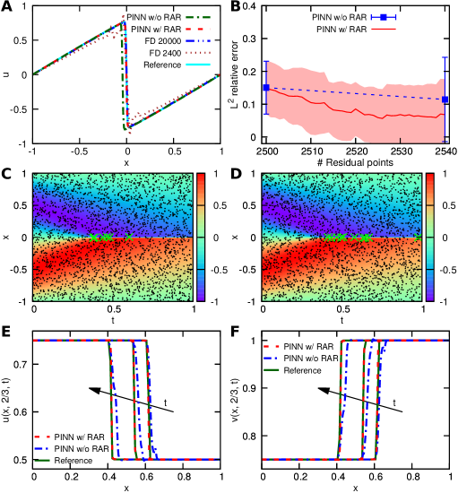
Figure 8: Example 4.2. Comparisons of the PINN solutions of (A, B, C and D) 1D and (E and F) 2D Burgers equations with and without RAR. (A) The cyan, green and red lines represent the reference solution of $u$ from [47], PINN solution without RAR, PINN solution with RAR at $t=0.9$, respectively. For the finite difference (FD) method, $200\times 100=20000$ spatial-temporal grid points are used to achieve a good solution (blue line). If only $60\times 40=2400$ points are used, the FD solution has large oscillations around the discontinuity (brown line). (B) $L^{2}$ relative error versus the number of residual points. The red solid line and shaded region correspond to the mean and one-standard-deviation band for the $L^{2}$ relative error of PINN with RAR, respectively. The blue dashed line is the mean and one-standard-deviation for the error of PINN using 2540 random residual points. The mean and standard deviation are obtained from 10 runs with random initial residual points. (C and D) Two representative examples for the residual points added via RAR. Black dots: initial residual points; green cross: added residual points; 6 and 11 residual points are added in C and D, respectively. (E and F) Comparison of the velocity profiles at $y=\frac{2}{3}$ from the PINNs with and without RAR for the 2D Burgers equation. The profiles at three different times ($t=0.2$, 0.5 and 1) are presented with $t$ increasing along the direction of the arrow.

4.3 Inverse problem for the Lorenz system

Consider the parameter identification problem of the following Lorenz system

$$\frac{dx}{dt}=\rho(y-x),\quad\frac{dy}{dt}=x(\sigma-z)-y,\quad\frac{dz}{dt}=xy-\beta z,$$

with the initial condition $(x(0),y(0),z(0))=(-8,7,27)$, where $\rho$, $\sigma$ and $\beta$ are the three parameters to be identified from the observations at certain times. The observations are produced by solving the above system to $t=3$ using Runge-Kutta (4,5) with the underlying true parameters $(\rho,\sigma,\beta)=(10,15,8/3)$. We choose 400 uniformly distributed random points and 25 equispaced points as the residual points $\mathcal{T}_{f}$ and $\mathcal{T}_{i}$, respectively. The evolution trajectories of $\rho$, $\sigma$ and $\beta$ are presented in Fig. 9A, with the final identified values of $(\rho,\sigma,\beta)=(10.002,14.999,2.668)$.

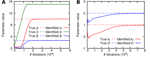
Figure 9: Examples 4.3 and 4.4. The identified values of (A) the Lorenz system and (B) diffusion-reaction system converge to the true values during the training process. The parameter values are scaled for plotting.

4.4 Inverse problem for diffusion-reaction systems

A diffusion-reaction system in porous media for the solute concentrations $C_{A}$, $C_{B}$ and $C_{C}$ ($A+2B\rightarrow C$) is described by

$$\frac{\partial C_{A}}{\partial t}=D\frac{\partial^{2}C_{A}}{\partial x^{2}}-k_{f}C_{A}C^{2}_{B},\quad\frac{\partial C_{B}}{\partial t}=D\frac{\partial^{2}C_{B}}{\partial x^{2}}-2k_{f}C_{A}C^{2}_{B},\quad x\in[0,1],t\in[0,10],$$

$$C_{A}(x,0)=C_{B}(x,0)=e^{-20x},\quad C_{A}(0,t)=C_{B}(0,t)=1,\quad C_{A}(1,t)=C_{B}(1,t)=0,$$

where $D=2\times 10^{-3}$ is the effective diffusion coefficient, and $k_{f}=0.1$ is the effective reaction rate. Because $D$ and $k_{f}$ depend on the pore structure and are difficult to measure directly, we estimate $D$ and $k_{f}$ based on 40000 observations of the concentrations $C_{A}$ and $C_{B}$ in the spatio-temporal domain. The identified $D$ ($1.98\times 10^{-3}$) and $k_{f}$ (0.0971) are displayed in Fig. 9B, which agree well with their true values.

4.5 Volterra IDE

Here, we consider the first-order integro-differential equation of the Volterra type in the domain $[0,5]$:

$$\frac{dy}{dx}+y(x)=\int_{0}^{x}e^{t-x}y(t)dt,\quad y(0)=1,$$

with the exact solution $y(x)=e^{-x}\cosh x.$ We solve this IDE using the method in Section 2.6, and approximate the integral using Gaussian-Legendre quadrature of degree 20. The $L^{2}$ relative error is $2\times 10^{-3}$, and the solution is shown in Fig. 10.

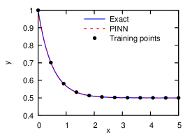
Figure 10: Example 4.5. The PINN algorithm for solving Volterra IDE. The blue solid line is the exact solution, and the red dash line is the numerical solution from PINN. 12 equispaced residual points (black dots) are used.

5 Concluding Remarks

In this paper, we present the algorithm, approximation theory, and error analysis of the physics-informed neural networks (PINNs) for solving different types of partial differential equations (PDEs). Compared to the traditional numerical methods, PINNs employ automatic differentiation to handle differential operators, and thus they are mesh-free. Unlike numerical differentiation, automatic differentiation does not differentiate the data and hence it can tolerate noisy data for training. We also discuss how to extend PINNs to solve other types of differential equations, such as integro-differential equations, and also how to solve inverse problems. In addition, we propose a residual-based adaptive refinement (RAR) method to improve the distribution of residual points during the training process, and thus increase the training efficiency.

To benefit both the education and the computational science communities, we have developed the Python library DeepXDE, an implementation of PINNs. By introducing the usage of DeepXDE, we show that DeepXDE enables user codes to be compact and follow closely the mathematical formulation. We also demonstrate how to customize DeepXDE to meet new problem requirements. Our numerical examples for forward and inverse problems verify the effectiveness of PINNs and the capability of DeepXDE. Scientific machine learning is emerging as a new and potentially powerful alternative to classical scientific computing, so we hope that libraries such as DeepXDE will accelerate this development and will make it accessible to the classroom but also to other researchers who may find the need to adopt PINN-like methods in their research, which can be very effective especially for inverse problems.

Despite the aforementioned advantages, PINNs still have some limitations. For forward problems, PINNs are currently slower than finite elements but this can be alleviated via offline training [58, 53]. For long time integration, one can also use time-parallel methods to simultaneously compute on multiple GPUs for shorter time domains. Another limitation is the search for effective neural network architectures, which is currently done empirically by users; however, emerging meta-learning techniques can be used to automate this search, see [59, 17]. Moreover, while here we enforce the strong form of PDEs, which is easy to be implemented by automatic differentiation, alternative weak/variational forms may also be effective, although they require the use of quadrature grids. Many other extensions for multi-physics and multi-scale problems are possible across different scientific disciplines by creatively designing the loss function and introducing suitable solution spaces. For instance, in the five examples we present here, we only assume data on scattered points, however, in geophysics or biomedicine we may have mixed data in the form of images and point measurements. In this case, we can design a composite neural network consisting of one convolutional neural network and one PINN sharing the same set of parameters, and minimize the total loss which could be a weighted summation of multiple losses from each neural network.

References

- [1] M. Abadi, P. Barham, J. Chen, Z. Chen, A. Davis, J. Dean, M. Devin, S. Ghemawat, G. Irving, M. Isard, et al., Tensorflow: A system for large-scale machine learning, in 12th USENIX Symposium on Operating Systems Design and Implementation, 2016, pp. 265–283.
- [2] M. Ainsworth and J. T. Oden, A posteriori error estimation in finite element analysis, vol. 37, John Wiley & Sons, 2011.
- [3] A. Baeza and P. Mulet, Adaptive mesh refinement techniques for high-order shock capturing schemes for multi-dimensional hydrodynamic simulations, International Journal for Numerical Methods in Fluids, 52 (2006), pp. 455–471.
- [4] N. Baker, F. Alexander, T. Bremer, A. Hagberg, Y. Kevrekidis, H. Najm, M. Parashar, A. Patra, J. Sethian, S. Wild, et al., Workshop report on basic research needs for scientific machine learning: Core technologies for artificial intelligence, tech. report, US DOE Office of Science, Washington, DC (United States), 2019.
- [5] A. G. Baydin, B. A. Pearlmutter, A. A. Radul, and J. M. Siskind, Automatic differentiation in machine learning: a survey, The Journal of Machine Learning Research, 18 (2017), pp. 5595–5637.
- [6] C. Beck, W. E, and A. Jentzen, Machine learning approximation algorithms for high-dimensional fully nonlinear partial differential equations and second-order backward stochastic differential equations, Journal of Nonlinear Science, (2017), pp. 1–57.
- [7] J. Berg and K. Nyström, A unified deep artificial neural network approach to partial differential equations in complex geometries, Neurocomputing, 317 (2018), pp. 28–41.
- [8] M. Betancourt, A geometric theory of higher-order automatic differentiation, arXiv preprint arXiv:1812.11592, (2018).
- [9] J. Bettencourt, M. J. Johnson, and D. Duvenaud, Taylor-mode automatic differentiation for higher-order derivatives in jax, (2019).
- [10] A. Blum and R. L. Rivest, Training a 3-node neural network is np-complete, in Advances in Neural Information Processing Systems, 1989, pp. 494–501.
- [11] L. Bottou and O. Bousquet, The tradeoffs of large scale learning, in Advances in Neural Information Processing Systems, 2008, pp. 161–168.
- [12] R. H. Byrd, P. Lu, J. Nocedal, and C. Zhu, A limited memory algorithm for bound constrained optimization, SIAM Journal on Scientific Computing, 16 (1995), pp. 1190–1208.
- [13] Y. Chen, L. Lu, G. E. Karniadakis, and L. D. Negro, Physics-informed neural networks for inverse problems in nano-optics and metamaterials, arXiv preprint arXiv:1912.01085, (2019).
- [14] P. G. Ciarlet, The finite element method for elliptic problems, vol. 40, Siam, 2002.
- [15] M. Dissanayake and N. Phan-Thien, Neural-network-based approximations for solving partial differential equations, Communications in Numerical Methods in Engineering, 10 (1994), pp. 195–201.
- [16] W. E and B. Yu, The deep Ritz method: A deep learning-based numerical algorithm for solving variational problems, Communications in Mathematics and Statistics, 6 (2018), pp. 1–12.
- [17] C. Finn, P. Abbeel, and S. Levine, Model-agnostic meta-learning for fast adaptation of deep networks, in Proceedings of the 34th International Conference on Machine Learning, 2017, pp. 1126–1135.
- [18] P. Grohs, F. Hornung, A. Jentzen, and P. Von Wurstemberger, A proof that artificial neural networks overcome the curse of dimensionality in the numerical approximation of black-scholes partial differential equations, arXiv preprint arXiv:1809.02362, (2018).
- [19] J. Han, A. Jentzen, and W. E, Solving high-dimensional partial differential equations using deep learning, Proceedings of the National Academy of Sciences, 115 (2018), pp. 8505–8510.
- [20] J. He, L. Li, J. Xu, and C. Zheng, ReLU deep neural networks and linear finite elements, arXiv preprint arXiv:1807.03973, (2018).
- [21] Q. He, D. Brajas-Solano, G. Tartakovsky, and A. M. Tartakovsky, Physics-informed neural networks for multiphysics data assimilation with application to subsurface transport, arXiv preprint arXiv:1912.02968, (2019).
- [22] T. J. Hughes, J. A. Cottrell, and Y. Bazilevs, Isogeometric analysis: Cad, finite elements, nurbs, exact geometry and mesh refinement, Computer methods in applied mechanics and engineering, 194 (2005), pp. 4135–4195.
- [23] A. D. Jagtap, K. Kawaguchi, and G. E. Karniadakis, Locally adaptive activation functions with slope recovery term for deep and physics-informed neural networks, arXiv preprint arXiv:1909.12228, (2019).
- [24] A. D. Jagtap, K. Kawaguchi, and G. E. Karniadakis, Adaptive activation functions accelerate convergence in deep and physics-informed neural networks, Journal of Computational Physics, 404 (2020), p. 109136.
- [25] P. Jin, L. Lu, Y. Tang, and G. E. Karniadakis, Quantifying the generalization error in deep learning in terms of data distribution and neural network smoothness, arXiv preprint arXiv:1905.11427, (2019).
- [26] C. Johnson, Numerical solution of partial differential equations by the finite element method, Courier Corporation, 2012.
- [27] G. E. Karniadakis and S. J. Sherwin, Spectral/hp element methods for computational fluid dynamics, Oxford University Press, second ed., 2013.
- [28] Y. Khoo, J. Lu, and L. Ying, Solving parametric PDE problems with artificial neural networks, arXiv preprint arXiv:1707.03351, (2017).
- [29] D. P. Kingma and J. Ba, Adam: A method for stochastic optimization, in International Conference on Learning Representations, 2015.
- [30] I. E. Lagaris, A. Likas, and D. I. Fotiadis, Artificial neural networks for solving ordinary and partial differential equations, IEEE Transactions on Neural Networks, 9 (1998), pp. 987–1000.
- [31] I. E. Lagaris, A. C. Likas, and D. G. Papageorgiou, Neural-network methods for boundary value problems with irregular boundaries, IEEE Transactions on Neural Networks, 11 (2000), pp. 1041–1049.
- [32] Y. LeCun, Y. Bengio, and G. Hinton, Deep learning, Nature, 521 (2015), p. 436.
- [33] Z. Long, Y. Lu, X. Ma, and B. Dong, PDE-net: Learning PDEs from data, in International Conference on Machine Learning, 2018, pp. 3214–3222.
- [34] L. Lu, P. Jin, and G. E. Karniadakis, DeepONet: Learning nonlinear operators for identifying differential equations based on the universal approximation theorem of operators, arXiv preprint arXiv:1910.03193, (2019).
- [35] L. Lu, Y. Shin, Y. Su, and G. E. Karniadakis, Dying ReLU and initialization: Theory and numerical examples, arXiv preprint arXiv:1903.06733, (2019).
- [36] L. Lu, Y. Su, and G. E. Karniadakis, Collapse of deep and narrow neural nets, arXiv preprint arXiv:1808.04947, (2018).
- [37] Z. Mao, A. D. Jagtap, and G. E. Karniadakis, Physics-informed neural networks for high-speed flows, Computer Methods in Applied Mechanics and Engineering, 360 (2020), p. 112789.
- [38] C. C. Margossian, A review of automatic differentiation and its efficient implementation, Wiley Interdisciplinary Reviews: Data Mining and Knowledge Discovery, 9 (2019), p. e1305.
- [39] A. J. Meade Jr and A. A. Fernandez, The numerical solution of linear ordinary differential equations by feedforward neural networks, Mathematical and Computer Modelling, 19 (1994), pp. 1–25.
- [40] X. Meng and G. E. Karniadakis, A composite neural network that learns from multi-fidelity data: Application to function approximation and inverse PDE problems, arXiv preprint arXiv:1903.00104, (2019).
- [41] M. A. Nabian and H. Meidani, A deep neural network surrogate for high-dimensional random partial differential equations, arXiv preprint arXiv:1806.02957, (2018).
- [42] G. Pang, L. Lu, and G. E. Karniadakis, fPINNs: Fractional physics-informed neural networks, SIAM Journal on Scientific Computing, 41 (2019), pp. A2603–A2626.
- [43] A. Paszke, S. Gross, S. Chintala, G. Chanan, E. Yang, Z. DeVito, Z. Lin, A. Desmaison, L. Antiga, and A. Lerer, Automatic differentiation in PyTorch, (2017).
- [44] A. Pinkus, Approximation theory of the MLP model in neural networks, Acta Numerica, 8 (1999), pp. 143–195.
- [45] T. Poggio, H. Mhaskar, L. Rosasco, B. Miranda, and Q. Liao, Why and when can deep-but not shallow-networks avoid the curse of dimensionality: a review, International Journal of Automation and Computing, 14 (2017), pp. 503–519.
- [46] N. Rahaman, A. Baratin, D. Arpit, F. Draxler, M. Lin, F. Hamprecht, Y. Bengio, and A. Courville, On the spectral bias of neural networks, in Proceedings of the 36th International Conference on Machine Learning, 2019, pp. 5301–5310.
- [47] M. Raissi, P. Perdikaris, and G. E. Karniadakis, Physics-informed neural networks: A deep learning framework for solving forward and inverse problems involving nonlinear partial differential equations, Journal of Computational Physics, 378 (2019), pp. 686–707.
- [48] M. Raissi, A. Yazdani, and G. E. Karniadakis, Hidden fluid mechanics: Learning velocity and pressure fields from flow visualizations, Science, (2020).
- [49] D. E. Rumelhart, G. E. Hinton, and R. J. Williams, Learning representations by back-propagating errors, Nature, 323 (1986), pp. 533–536.
- [50] J. Sirignano and K. Spiliopoulos, DGM: A deep learning algorithm for solving partial differential equations, Journal of Computational Physics, 375 (2018), pp. 1339–1364.
- [51] A. M. Tartakovsky, C. O. Marrero, P. Perdikaris, G. D. Tartakovsky, and D. Barajas-Solano, Learning parameters and constitutive relationships with physics informed deep neural networks, arXiv preprint arXiv:1808.03398, (2018).
- [52] B. P. van Milligen, V. Tribaldos, and J. Jiménez, Neural network differential equation and plasma equilibrium solver, Physical Review Letters, 75 (1995), p. 3594.
- [53] N. Winovich, K. Ramani, and G. Lin, ConvPDE-UQ: Convolutional neural networks with quantified uncertainty for heterogeneous elliptic partial differential equations on varied domains, Journal of Computational Physics, 394 (2019), pp. 263–279.
- [54] Z.-Q. J. Xu, Y. Zhang, T. Luo, Y. Xiao, and Z. Ma, Frequency principle: Fourier analysis sheds light on deep neural networks, arXiv preprint arXiv:1901.06523, (2019).
- [55] L. Yang, D. Zhang, and G. E. Karniadakis, Physics-informed generative adversarial networks for stochastic differential equations, arXiv preprint arXiv:1811.02033, (2018).
- [56] D. Zhang, L. Guo, and G. E. Karniadakis, Learning in modal space: Solving time-dependent stochastic PDEs using physics-informed neural networks, arXiv preprint arXiv:1905.01205, (2019).
- [57] D. Zhang, L. Lu, L. Guo, and G. E. Karniadakis, Quantifying total uncertainty in physics-informed neural networks for solving forward and inverse stochastic problems, Journal of Computational Physics, 397 (2019), p. 108850.
- [58] Y. Zhu, N. Zabaras, P.-S. Koutsourelakis, and P. Perdikaris, Physics-constrained deep learning for high-dimensional surrogate modeling and uncertainty quantification without labeled data, arXiv preprint arXiv:1901.06314, (2019).
- [59] B. Zoph and Q. V. Le, Neural architecture search with reinforcement learning, arXiv preprint arXiv:1611.01578, (2016).