Bayesian Inference for Regression Copulas

$\mbox{}^{\star}$Correspondence should be directed to Nadja Klein at Humboldt Universität zu Berlin, Unter den Linden 6, 10099 Berlin. Email: nadja.klein@hu-berlin.de. Michael Stanley Smith is Professor of Management (Econometrics) at Melbourne Business School, University of Melbourne. Nadja Klein is an Assistant Professor of Applied Statistics at Humboldt Universität zu Berlin. Nadja Klein gratefully acknowledges funding from the Alexander von Humboldt foundation and the German research foundation (DFG) through the Emmy Noether grant KL 3037/1-1. The authors thank the Editor, Associate Editor and three referees whose comments improved the paper.

We propose a new semi-parametric distributional regression smoother that is based on a copula decomposition of the joint distribution of the vector of response values. The copula is high-dimensional and constructed by inversion of a pseudo regression, where the conditional mean and variance are semi-parametric functions of covariates modeled using regularized basis functions. By integrating out the basis coefficients, an implicit copula process on the covariate space is obtained, which we call a ‘regression copula’. We combine this with a non-parametric margin to define a copula model, where the entire distribution—including the mean and variance—of the response is a smooth semi-parametric function of the covariates. The copula is estimated using both Hamiltonian Monte Carlo and variational Bayes; the latter of which is scalable to high dimensions. Using real data examples and a simulation study we illustrate the efficacy of these estimators and the copula model. In a substantive example, we estimate the distribution of half-hourly electricity spot prices as a function of demand and two time covariates using radial bases and horseshoe regularization. The copula model produces distributional estimates that are locally adaptive with respect to the covariates, and predictions that are more accurate than those from benchmark models.

Keywords: Distributional regression; Hamiltonian Monte Carlo; Implicit copula, P-splines; Radial basis functions, Variational Bayes.

1 Introduction

Non- or semi-parametric regression methods typically estimate only the mean of a response variable as an unknown smooth function of covariates. Yet in many applications, other features of the response distributions—such as higher moments and quantiles—also vary with the covariates. For example, to address this Rigby and Stasinopoulos (2005) and Klein et al. (2015) make all the parameters of a response distribution unknown smooth functions of the covariates. However, these authors assume a specific parametric distribution for the response, conditional on the functions. In this paper, we propose a novel class of semi-parametric distributional regression models for continuous data that avoids such an assumption. It uses a copula decomposition of the joint distribution of a vector of values from a single response variable. To do so, we employ a new copula with a dependence structure that is an unknown smooth function of the covariate values, and model the marginal distribution of the response variable non-parametrically. The distributional regression is therefore flexible in two ways: non-parametric in a distributional sense with respect to the margin of the response, and semi-parametric in a functional sense with respect to the covariates via the copula. It allows the entire distribution of the response to be a smooth unknown function of the covariates.

Copula models (McNeil et al., 2005; Nelsen, 2006) are popular because the marginal distributions can be modeled arbitrarily and separately from the dependence structure. In this paper, the copula has dimension equal to the length of the vector of response values, which can be high ($87,648$ in one of our examples). Few existing copulas can be used in such a situation, although copulas constructed by the inversion of a parametric distribution (Nelsen, 2006, Sec. 3.1) can. Such copulas are called either ‘inversion’ or ‘implicit’ copulas, and those constructed by the inversion of Gaussian (Song, 2000), t (Demarta and McNeil, 2005) and skew t (Smith et al., 2012) distributions are popular. More flexible implicit copulas can be constructed by inverting the distribution of values of one or more response variables from parametric statistical models. We label these response variables ‘pseudo-responses’ because they are not observed directly. Examples include implicit copulas constructed from factor models (Murray et al., 2013; Oh and Patton, 2017), vector autoregressions (Smith and Vahey, 2016), nonlinear state space models (Smith and Maneesoonthorn, 2018), Gaussian processes (Wauthier and Jordan, 2010; Wilson and Ghahramani, 2010) and regularized regression (Klein and Smith, 2018). These implicit copulas reproduce the dependence structure of the pseudo-response variables, and combining them with arbitrary margins produces a more flexible model that allows for a wide range of data distributions.

In this paper we show how to construct an implicit copula from a heteroscedastic semi-parametric regression. Both the mean and variance of the pseudo-response are unknown smooth functions of covariates, each modeled using function bases with regularized coefficients. Because implicit copulas do not retain any information about the marginal (i.e. unconditional on the covariates) location and scale of the pseudo-response, we normalize the pseudo-response to have zero mean and unit variance marginally. By integrating out the basis coefficients of the functions, we derive a copula that is a smooth function of the covariate values and regularization parameters only. We call this a ‘regression copula’, because when used in a copula model for the vector of response values, it captures the effect of the covariates. The regularization parameters become the copula parameters, and these require estimation.

There are two main challenges when estimating the copula parameters: (i) the copula function and density are unavailable in closed form, and (ii) the copula has dimension equal to the sample size, which may be high. We outline two Bayesian approaches to overcome these challenges. The first is a Markov chain Monte Carlo (MCMC) sampler with a Hamiltonian Monte Carlo step (Neal, 2011; Hoffman and Gelman, 2014) to evaluate the posterior distribution exactly. The second is a variational Bayes (VB) estimator (Jordan et al., 1999; Ormerod and Wand, 2010) to compute approximate posterior inference quickly when the sample size and dimension are high. The VB estimator is based on a Gaussian approximation with a sparse factor representation of its covariance matrix (Ong et al., 2018). We calibrate this using stochastic gradient ascent (Honkela et al., 2010; Salimans and Knowles, 2013) with gradient estimates computed efficiently (Kingma and Welling, 2014). The result is a VB estimator for the regression copula that is applicable to large datasets and is accurate in our empirical work.

We derive properties of the regression copula, including dependence metrics, and show that the independence copula is a limiting case. The entire (Bayesian posterior) predictive distribution of the observed response variable can be computed from the copula model. This distribution is a smooth function of the covariates, and its first and second moments are estimates of the regression and variance functions. The inclusion of a heteroscedastic term for the pseudo-response produces a regression copula that is a more flexible function of the covariates than the implicit copula of a homoscedastic regression discussed by Klein and Smith (2018). This results in predictive density and regression mean and variance function estimates for the observed response with levels of smoothing that are ‘locally adaptive’ with respect to the covariates. Such local adaptivity is difficult to achieve in alternative approaches to distributional regression.

We first demonstrate the efficacy of our approach using four real univariate datasets. Each has a response with a margin that is non-Gaussian that we estimate non-parametrically. The unknown smooth functions are modeled using B-spline bases and autoregressive priors for the coefficients. The estimated regression and variance functions of the response from the copula model are nonlinearly related to the covariates. Their estimates using the exact and approximate posteriors prove very similar, yet the latter are faster to evaluate using VB. A simulation study based on fitting distributional regressions to these four datasets, shows that the proposed regression copula model produces more accurate density forecasts than that proposed by Klein and Smith (2018), a P-spline regression with Gaussian disturbances, a heteroscedastic P-spline regression, and the most likely transformation estimator of Hothorn et al. (2017).

Distributional regression can be used to estimate the relationship between intraday electricity prices and exogenous drivers (Gianfreda and Bunn, 2018). We apply our approach to a distributional regression for $n=87,648$ half-hourly electricity spot prices in the Australian National Electricity Market (NEM) between 2014 and 2018. There are three covariates (demand, time of day and day) and the unknown smooth functions are modeled using trivariate radial bases, along with horseshoe priors to regularize the coefficients. The resulting regression copula model links the entire distribution of prices to the three covariates. By adjusting the radial bases so that they are periodic in the time of day covariate (only), the price distribution is also periodic in this covariate. The fitted regression copula model captures the changing impact of demand on the price distribution at different times of the day and over the four year period. Using cross-validated density forecasting metrics and the quantile score (Gneiting and Ranjan, 2011), we show the copula model is more accurate than two benchmark distributional regression methods.

Finally, we note here that copulas have been used extensively in multivariate regression frameworks, although our approach is very different in two ways. First, previous approaches use a low-dimensional copula to capture the dependence between multiple response variables with regression margins, which is often called a ‘copula regression’ (Pitt et al., 2006), whereas we use a copula to capture the dependence between different observations on a single response variable. Second, most previous methods employ elliptical or vine (Aas et al., 2009) copulas with closed form densities. In contrast, while our copula does not have a closed form density, it is tractable and scalable to higher dimensions, as illustrated in our empirical work.

The paper is structured as follows. Sec. 2.1 shows how to construct a distributional regression model using a regression copula and an arbitrary margin. Our regression copula is outlined in Sec. 2.2, along with some of its properties in Sec. 2.3. Sec. 3 outlines exact and approximate Bayesian posterior estimators, along with distribution and functional prediction. Sec. 4 discusses the four univariate real data examples and the comparison with benchmark alternatives via simulation. Sec. 5 contains the application to electricity prices, and Sec. 6 concludes.

2 Distributional Regression using Implicit Copulas

In this section we first introduce the copula model used for distributional regression. Then we outline our proposed implicit copula, along with some of its key properties.

2.1 Copula model

Consider $N$ realizations $\bm{Y}_{(N)}=(Y_{1},\ldots,Y_{N})^{\prime}$ of a continuous-valued response, with corresponding covariate values $\tilde{\text{\boldmath$x$}}_{(N)}=\{\tilde{\text{\boldmath$x$}}_{1},\ldots,\tilde{\text{\boldmath$x$}}_{N}\}$. Following Sklar’s Theorem, the joint density of $\bm{Y}_{(N)}|\tilde{\text{\boldmath$x$}}_{(N)}$ can always be written as

$$p(\text{\boldmath$y$}_{(N)}|\tilde{\text{\boldmath$x$}}_{(N)})=c^{\dagger}(F(y_{1}|\tilde{\text{\boldmath$x$}}_{1}),\ldots,F(y_{N}|\tilde{\text{\boldmath$x$}}_{N})|\tilde{\text{\boldmath$x$}}_{(N)})\prod_{i=1}^{N}p(y_{i}|\tilde{\text{\boldmath$x$}}_{i})\,,\;\;\mbox{ for }N\geq 2\,.$$

Here, $c^{\dagger}$ is the density of an $N$-dimensional copula process, and $F(y_{i}|\tilde{\text{\boldmath$x$}}_{i})$ is the distribution function of $Y_{i}|\tilde{\text{\boldmath$x$}}_{i}$; both of which are unknown. In this paper we approximate this joint distribution, also conditional on copula parameters $\theta$, with the copula model

$$p(\text{\boldmath$y$}_{(N)}|\tilde{\text{\boldmath$x$}}_{(N)},\text{\boldmath$\theta$})=c_{H}\left(F_{Y}(y_{1}),\ldots,F_{Y}(y_{N})|\tilde{\text{\boldmath$x$}}_{(N)},\text{\boldmath$\theta$}\right)\prod_{i=1}^{N}p_{Y}(y_{i})\,.$$ (1)

The distribution $Y_{i}|\tilde{\text{\boldmath$x$}}_{i}$ is assumed to be invariant with respect to $\tilde{\text{\boldmath$x$}}_{i}$, and has density $p_{Y}$ and distribution function $F_{Y}$. However, the impact of the covariate values on $\bm{Y}_{(N)}$ is captured by the copula with density $c_{H}(\text{\boldmath$u$}_{(N)}|\tilde{\text{\boldmath$x$}}_{(N)},\text{\boldmath$\theta$})$, where $\text{\boldmath$u$}_{(N)}=(u_{1},\ldots,u_{N})^{\prime}$ and $u_{i}=F_{Y}(y_{i})$. We call this a ‘regression copula’ because it is a function of $\tilde{\text{\boldmath$x$}}_{(N)}$. It is a copula process on the covariate space with parameters $\theta$ that do not vary with $N$. We use the implicit copula proposed in the sub-section below for $c_{H}$, and a major aim of this paper is to show that by doing so, adopting Eq. (1) provides a very flexible, but tractable, approach to distributional regression.

Before specifying $c_{H}$, we stress that even though $Y_{i}|\tilde{\text{\boldmath$x$}}_{i}$ is assumed invariant with respect to $\tilde{\text{\boldmath$x$}}_{i}$, $Y_{i}$ is not marginally independent of $\tilde{\text{\boldmath$x$}}_{i}$ when also conditioning on the unknown mean and variance functions of the pseudo-response, as shown in Part A.1 of the Web Appendix. Moreover, to see how the response is affected by the covariates in the distributional regression at Eq.(1), consider a sample of size $n$ with $\text{\boldmath$y$}=(y_{1},\ldots,y_{n})^{\prime}$, covariate values $\tilde{\text{\boldmath$x$}}=\{\tilde{\text{\boldmath$x$}}_{1},\ldots,\tilde{\text{\boldmath$x$}}_{n}\}$ and $\text{\boldmath$u$}=(u_{1},\ldots,u_{n})^{\prime}$. Then a new response $Y_{n+1}$ with corresponding covariate values $\tilde{\text{\boldmath$x$}}_{n+1}$ has predictive density

$$p(y_{n+1}|\tilde{\text{\boldmath$x$}}_{(n+1)},\text{\boldmath$\theta$})=\int p(\text{\boldmath$y$},y_{n+1}|\tilde{\text{\boldmath$x$}}_{(n+1)},\text{\boldmath$\theta$})\mbox{d}\text{\boldmath$y$}=\int c_{H}(\text{\boldmath$u$}_{(n+1)}|\tilde{\text{\boldmath$x$}}_{(n+1)},\text{\boldmath$\theta$})\mbox{d}\text{\boldmath$u$}\,p_{Y}(y_{n+1})\,.$$ (2)

This density is a function of all the covariate values $\tilde{\text{\boldmath$x$}}_{(n+1)}=\{\tilde{\text{\boldmath$x$}},\tilde{\text{\boldmath$x$}}_{n+1}\}$, which includes $\tilde{\text{\boldmath$x$}}_{n+1}$. Moreover, integrating over the posterior of $\theta$ gives the posterior predictive density of $Y_{n+1}$ from the regression model as

$$p(y_{n+1}|\tilde{\text{\boldmath$x$}}_{(n+1)},\bm{y})=\int p(y_{n+1}|\tilde{\text{\boldmath$x$}}_{(n+1)},\text{\boldmath$\theta$})p(\text{\boldmath$\theta$}|\text{\boldmath$y$})\mbox{d}\text{\boldmath$\theta$}\,.$$ (3)

Eq. (3) forms the basis for our distributional regression predictions as a function of $\tilde{\text{\boldmath$x$}}_{n+1}$, and its first two moments are estimates of the regression mean and variance functions. In Sec. 3.4 we show how to compute Eq. (2) and Eq. (3) efficiently for our proposed copula.

2.2 Implicit regression copula

Key to our approach is the regression copula with density $c_{H}$, which is derived from a semi-parametric heteroscedastic regression model for a pseudo-response. To do so, we first outline the regression and then construct its implicit copula with only the basis coefficients of the mean function integrated out, which is a Gaussian copula. Next, to derive the copula with the basis coefficients of the variance function also integrated out, it is represented as an integral of the Gaussian copula. We show that such a representation is computationally efficient.

2.2.1 Pseudo-response regression model

Consider a regression model for a pseudo-response $\tilde{Z}_{i}$ with covariates $\tilde{\text{\boldmath$x$}}_{i}=\{\bm{x}_{i},\bm{w}_{i}\}$ given by

$$\tilde{Z}_{i} = \tilde{m}(\bm{x}_{i})+\varepsilon_{i}\,,\;\;\varepsilon_{i}\sim N(0,\sigma^{2}\sigma^{2}_{i})\,,$$

$$\sigma^{2}_{i} = \exp(g(\bm{w}_{i}))\,,\mbox{ for }i=1,\ldots,n\,,$$ (4)

where the first and second moments are smooth unknown functions $\tilde{m}$ and $g$ of the two covariate vectors. We model these using linear combinations of basis functions $b_{1},\ldots,b_{p_{1}}$ and $v_{1},\ldots,v_{p_{2}}$, such that $\tilde{m}(\bm{x})=\sum_{j=1}^{p_{1}}\beta_{j}b_{j}(\bm{x})$ and $g(\bm{w})=\sum_{j=1}^{p_{2}}\alpha_{j}v_{j}(\bm{w})$. Typical choices for the bases include polynomial or B-spline bases for a scalar covariate, and additive or radial bases for multiple covariates. With these approximations, the regression model is usually called semi-parametric.

For $n$ pseudo-response values $\tilde{\bm{Z}}=(\tilde{Z}_{1},\ldots,\tilde{Z}_{n})^{\prime}$ the regression at Eq. (2.2.1) can be written as

$$\tilde{\bm{Z}} =B\text{\boldmath$\beta$}+\text{\boldmath$\varepsilon$}\,,\;\;\text{\boldmath$\varepsilon$}=(\varepsilon_{1},\ldots,\varepsilon_{n})^{\prime}\sim N(0,\sigma^{2}\Sigma)\,,$$ (5)

$$\Sigma =\operatorname{diag}(\sigma_{1}^{2},\ldots,\sigma_{n}^{2})\,,\mbox{ }\sigma_{i}^{2}=\exp(\text{\boldmath$v$}_{i}^{\prime}\text{\boldmath$\alpha$}),\mbox{ for }i=1,\ldots,n\,,$$

where $\text{\boldmath$\beta$}=(\beta_{1},\ldots,\beta_{p_{1}})^{\prime}$, $\text{\boldmath$\alpha$}=(\alpha_{1},\ldots,\alpha_{p_{2}})^{\prime}$, and the design matrices $B\in\text{$\mathds{R}$}^{n\times p_{1}}$ and $V\in\text{$\mathds{R}$}^{n\times p_{2}}$ have $i$th rows $\text{\boldmath$b$}_{i}^{\prime}=(b_{1}(\bm{x}_{i}),\ldots,b_{p_{1}}(\bm{x}_{i}))$ and $\text{\boldmath$v$}_{i}^{\prime}=(v_{1}(\bm{w}_{i}),\ldots,v_{p_{2}}(\bm{w}_{i}))$, respectively. To produce smooth and efficient function estimates it is usual to regularize the basis coefficients $\beta$ and $\alpha$. In a conjugate Bayesian context, this corresponds to adopting the conditionally Gaussian priors

$$\text{\boldmath$\beta$}|\text{\boldmath$\theta$}_{\beta},\sigma^{2}\sim N\left(\mathbf{0},\sigma^{2}P_{\beta}(\text{\boldmath$\theta$}_{\beta})^{-1}\right)\,,\;\;\;\text{\boldmath$\alpha$}|\text{\boldmath$\theta$}_{\alpha}\sim N\left(\mathbf{0},P_{\alpha}(\text{\boldmath$\theta$}_{\alpha})^{-1}\right)\,,$$ (6)

with smoothing (or ‘hyper’) parameters $\text{\boldmath$\theta$}_{\beta}$ and $\text{\boldmath$\theta$}_{\alpha}$. The forms of the precision matrices $P_{\beta},P_{\alpha}$ are typically matched with the choice of bases for $\tilde{m}$ and $g$, for which we give two examples later.

2.2.2 Regression copula construction

We extract two copulas from the regression model defined at Eq. (2.2.1)–(6). They are called ‘implicit’ (McNeil et al., 2005, p.190) or ‘inversion’ (Nelsen, 2006, p.51) copulas because they are constructed by inverting Sklar’s theorem. The copulas are $n$-dimensional with dependence structures that are (smooth) functions of $\tilde{\text{\boldmath$x$}}=\{\text{\boldmath$x$},\text{\boldmath$w$}\}$, with $\text{\boldmath$x$}=(\bm{x}_{1}^{\prime},\ldots,\bm{x}_{n}^{\prime})^{\prime}$ and $\text{\boldmath$w$}=(\bm{w}_{1}^{\prime},\ldots,\bm{w}_{n}^{\prime})^{\prime}$.

The first regression copula derived is the implicit copula of the distribution $\tilde{\bm{Z}}|\text{\boldmath$x$},\text{\boldmath$w$},\sigma^{2},\text{\boldmath$\alpha$},\text{\boldmath$\theta$}_{\beta},\text{\boldmath$\theta$}_{\alpha}$, which we label $C_{1}$. To construct $C_{1}$, note that the prior for $\beta$ is conjugate and can be integrated out of the distribution for $\tilde{\bm{Z}}$ analytically, giving

$$\tilde{\text{\boldmath$Z$}}|\text{\boldmath$x$},\text{\boldmath$w$},\sigma^{2},\text{\boldmath$\alpha$},\text{\boldmath$\theta$}_{\beta},\text{\boldmath$\theta$}_{\alpha}\sim\operatorname{N}(\mathbf{0},\sigma^{2}[\Sigma^{-1}-\Sigma^{-1}B\Omega B^{\prime}\Sigma^{-1}]^{-1})\,,$$ (7)

where $\Omega=\left(B^{\prime}\Sigma^{-1}B+P_{\beta}(\text{\boldmath$\theta$}_{\beta})\right)^{-1}$, and by applying the Woodbury formula

$$[\Sigma^{-1}-\Sigma^{-1}B\Omega B^{\prime}\Sigma^{-1}]^{-1}=\Sigma+BP_{\beta}(\text{\boldmath$\theta$}_{\beta})^{-1}B^{\prime}.$$

It is straightforward to show that the copula of a normal distribution is the widely employed Gaussian copula (Song, 2000). It is obtained by standardizing the marginal means to zero and the variances to one. The margin in $\tilde{Z}_{i}$ at Eq. (7) is $\operatorname{N}(0,\sigma^{2}[\exp(\text{\boldmath$v$}^{\prime}_{i}\text{\boldmath$\alpha$})+\text{\boldmath$b$}^{\prime}_{i}P_{\beta}(\text{\boldmath$\theta$}_{\beta})^{-1}\text{\boldmath$b$}_{i}])$, so that we normalize $\tilde{\text{\boldmath$Z$}}$ by the diagonal matrix $\sigma^{-1}S(\text{\boldmath$x$},\text{\boldmath$w$},\text{\boldmath$\alpha$},\text{\boldmath$\theta$}_{\beta})=\sigma^{-1}\operatorname{diag}(s_{1},\ldots,s_{n})$ with $s_{i}=[\exp(\text{\boldmath$v$}^{\prime}_{i}\text{\boldmath$\alpha$})+\text{\boldmath$b$}^{\prime}_{i}P_{\beta}(\text{\boldmath$\theta$}_{\beta})^{-1}\text{\boldmath$b$}_{i}]^{-1/2}$, to get $\text{\boldmath$Z$}=\sigma^{-1}S(\text{\boldmath$x$},\text{\boldmath$w$},\text{\boldmath$\alpha$},\text{\boldmath$\theta$}_{\beta})\tilde{\text{\boldmath$Z$}}$ . With this, the regression at Eq. (2.2.1) can be re-written for the standardized pseudo-response as

$$Z_{i}=m(\bm{x}_{i},\bm{w}_{i})+\frac{s_{i}}{\sigma}\varepsilon_{i}\,,\;\;\varepsilon_{i}\sim N(0,\sigma^{2}\sigma_{i}^{2})\,,$$ (8)

where $m(\bm{x}_{i},\bm{w}_{i})=(s_{i}/\sigma)\tilde{m}(\bm{x}_{i})=(s_{i}/\sigma)\bm{b}_{i}^{\prime}\text{\boldmath$\beta$}$ is a function of both $\bm{x}_{i}$ and $\bm{w}_{i}$, because $s_{i}$ is also.

Denoting $S\equiv S(\text{\boldmath$x$},\text{\boldmath$w$},\text{\boldmath$\alpha$},\text{\boldmath$\theta$}_{\beta})$ for conciseness, the distribution of the normalized vector with $\beta$ integrated out is

$$\text{\boldmath$Z$}|\text{\boldmath$x$},\text{\boldmath$w$},\sigma^{2},\text{\boldmath$\alpha$},\text{\boldmath$\theta$}_{\beta},\text{\boldmath$\theta$}_{\alpha} \sim N(\bm{0},R)\,,\mbox{ with}$$

$$R\equiv R(\text{\boldmath$x$},\text{\boldmath$w$},\text{\boldmath$\alpha$},\text{\boldmath$\theta$}_{\beta}) = S(\Sigma+BP_{\beta}(\text{\boldmath$\theta$}_{\beta})^{-1}B^{\prime})S\,,$$ (9)

and $N(0,1)$ margins for all elements $Z_{1},\ldots,Z_{n}$. It is straightforward to show (Song, 2000) that the random vectors $\tilde{\bm{Z}}$ and $\bm{Z}$ (conditional on $\text{\boldmath$x$},\text{\boldmath$w$},\text{\boldmath$\alpha$},\text{\boldmath$\theta$}_{\beta}$) have the same Gaussian copula function

$$C_{1}(\bm{u}|\bm{x},\text{\boldmath$w$},\text{\boldmath$\alpha$},\text{\boldmath$\theta$}_{\beta})=\Phi\left(\Phi_{1}^{-1}(u_{1}),\ldots,\Phi_{1}^{-1}(u_{n});\bm{0},R\right)\,,$$

where $\bm{u}=(u_{1},\ldots,u_{n})^{\prime}$, and $\Phi(\cdot;\bm{0},R)$ and $\Phi_{1}$ are the distribution functions of $N(\bm{0},R)$ and $N(0,1)$ distributions, respectively. This is a regression copula because $R$ is a function of $\tilde{\text{\boldmath$x$}}$.

We make a number of observations on $C_{1}$. First, the parameter $\sigma^{2}$ does not feature in the expression for $R$, and is unidentified in the copula, so that we set $\sigma^{2}=1$ throughout the paper. Second, if the density of the distribution for $Z$ at Eq. (9) is denoted as $p_{Z}$, with marginal densities $p_{Z_{i}}$ for $i=1,\ldots,n$, then the copula density $c_{1}=\frac{\partial^{n}}{\partial u_{1}\ldots\partial u_{n}}C_{1}$ is

$$c_{1}(\bm{u}|\bm{x},\text{\boldmath$w$},\text{\boldmath$\alpha$},\text{\boldmath$\theta$}_{\beta})=\frac{p_{Z}(\text{\boldmath$z$}|\text{\boldmath$x$},\text{\boldmath$w$},\text{\boldmath$\alpha$},\text{\boldmath$\theta$}_{\beta})}{\prod_{i=1}^{n}p_{Z_{i}}(z_{i}|\text{\boldmath$x$},\text{\boldmath$w$},\text{\boldmath$\alpha$},\text{\boldmath$\theta$}_{\beta})}=\frac{\phi(\text{\boldmath$z$};\bm{0},R)}{\prod_{i=1}^{n}\phi_{1}(z_{i})},$$ (10)

where $z_{i}=\Phi^{-1}_{1}(u_{i})$, $\text{\boldmath$z$}=(z_{1},\ldots,z_{n})^{\prime}$, and $\phi(\cdot;\bm{0},R)$ and $\phi_{1}$ are the densities of $N(\bm{0},R)$ and $N(0,1)$ distributions, respectively. Third, if a non-conjugate prior is used for $\bm{\beta}$, then $C_{1}$ is not a Gaussian copula (something we do not consider in this paper). Last, because $R$ is a function of $\alpha$, so is the dependence structure of $C_{1}$. If $\text{\boldmath$\alpha$}=\bm{0}$, then $C_{1}$ corresponds to the copula of a homoscedastic regression, as discussed by Klein and Smith (2018).

The second regression copula derived is the implicit copula of $\bm{Z}$ with both $\beta$ and $\alpha$ integrated out. We label this $C_{H}$ (for heteroscedastic regression copula), and it is this copula with density $c_{H}$ that is used to model the observed data at Eq. (1).

Theorem 1 (Definition of $C_{H}$ and $c_{H}$).

If $\tilde{Z}_{i}$ follows the heteroscedastic regression for the pseudo-response at Eq. (2.2.1)–(6), $Z_{i}=s_{i}\tilde{Z}_{i}$ is the normalized response at Eq. (8) with $\sigma=1$, $\tilde{\text{\boldmath$x$}}=\{\text{\boldmath$x$},\text{\boldmath$w$}\}$ are the covariate values and $\text{\boldmath$\theta$}=\{\text{\boldmath$\theta$}_{\beta},\text{\boldmath$\theta$}_{\alpha}\}$, then the $n$-dimensional implicit copula of the distribution $\bm{Z}|\tilde{\text{\boldmath$x$}},\text{\boldmath$\theta$}$ has density

$$c_{H}(\bm{u}|\tilde{\text{\boldmath$x$}},\text{\boldmath$\theta$})=\int c_{1}(\bm{u}|\bm{x},\bm{w},\text{\boldmath$\alpha$},\bm{\theta}_{\beta})p(\text{\boldmath$\alpha$}|\text{\boldmath$\theta$}_{\alpha})\mathrm{d}\text{\boldmath$\alpha$}=\frac{\int\phi(\text{\boldmath$z$};\bm{0},R)p(\text{\boldmath$\alpha$}|\text{\boldmath$\theta$}_{\alpha})\mathrm{d}\text{\boldmath$\alpha$}}{\prod_{i=1}^{n}\phi_{1}(z_{i})}\,,$$

and copula function

$$C_{H}(\bm{u}|\tilde{\text{\boldmath$x$}},\text{\boldmath$\theta$})=\int C_{1}(\bm{u}|\bm{x},\bm{w},\text{\boldmath$\alpha$},\bm{\theta}_{\beta})p(\text{\boldmath$\alpha$}|\text{\boldmath$\theta$}_{\alpha})\mathrm{d}\text{\boldmath$\alpha$}=\int\Phi(\bm{z};0,R)p(\text{\boldmath$\alpha$}|\text{\boldmath$\theta$}_{\alpha})\mathrm{d}\text{\boldmath$\alpha$}\,,$$

where $\text{\boldmath$u$}=(u_{1},\ldots,u_{n})^{\prime}$, the marginal $u_{i}=F(z_{i}|\tilde{\text{\boldmath$x$}},\text{\boldmath$\theta$})=\Phi_{1}(z_{i})$, so that $z_{i}=\Phi_{1}^{-1}(u_{i})$.
Proof: See Part A of the Web Appendix.

We make three observations on $C_{H}$ defined in Theorem 1. First, integration over $\alpha$ is required to compute $C_{H}$ and $c_{H}$. In Sec. 3 we show how to do this integration exactly using Hamiltonian Monte Carlo (HMC), and approximately using variational Bayes (VB) methods, when computing posterior inference. Second, the dependence parameters of $C_{H}$ are the the smoothing parameters $\text{\boldmath$\theta$}=\{\text{\boldmath$\theta$}_{\alpha},\text{\boldmath$\theta$}_{\beta}\}$ of $\tilde{m},g$ in the regression for the pseudo-response at Eq. (2.2.1). Last, it is much simpler to construct the implicit copula of $\bm{Z}$, rather than $\tilde{\bm{Z}}$ here. This is because constructing the latter copula would involve evaluating (and inverting) the $n$ marginal distribution functions

$$\tilde{F}_{i}(\tilde{z}_{i}|\tilde{\text{\boldmath$x$}},\text{\boldmath$\theta$})=\int\Phi_{1}(\tilde{z}_{i}/s_{i})p(\text{\boldmath$\alpha$}|\text{\boldmath$\theta$}_{\alpha})\mbox{d}\text{\boldmath$\alpha$}\,,\;i=1,\ldots,n\,.$$

Each of these involves computing a $p_{2}$-dimensional integral using numerical methods. In contrast, the margin of $Z_{i}|\tilde{\text{\boldmath$x$}},\text{\boldmath$\theta$}$ is simply a standard normal, which greatly simplifies evaluation of $C_{H}$.

2.3 Properties of $C_{H}$

Here, we state some properties of the regression copula $C_{H}$. First, the independence copula is a limiting case of this copula, as outlined in Theorem 2 below:

Theorem 2.

Let $\Pi(\text{\boldmath$u$})=\prod_{i=1}^{n}u_{i}$ be the independence copula function (Nelsen, 2006, p.11), and $\gamma_{\beta}(\text{\boldmath$\theta$}_{\beta})<\infty$ be the maximum marginal variance of the prior for $\beta$ at Eq. (6), then

$$\lim\limits_{\gamma_{\beta}\rightarrow 0}C_{H}(\text{\boldmath$u$}|\tilde{\text{\boldmath$x$}},\text{\boldmath$\theta$})=\Pi(\text{\boldmath$u$})\,.$$

Proof: See Part A of the Web Appendix.

An implication of Theorem 2 is that the relationship between the response and covariates is weak when the posterior of $\gamma_{\beta}$ is close to zero.

Below we give expressions for some common dependence metrics of the bivariate sub-copula $C_{H}^{ij}$ of $C_{H}$ in elements $1\leq i<j\leq n$. The derivations are given in Part A of the Web Appendix.

• For $q\in(0,1)$, if $(U_{i},U_{j})\sim C^{ij}_{H}$, the lower and upper quantile dependence are

  $$\lambda^{L}_{ij}(q|\tilde{\text{\boldmath$x$}},\text{\boldmath$\theta$}) \equiv \mbox{Pr}(U_{i}<q|U_{j}<q)=\int\lambda^{L}_{1,ij}(q|\text{\boldmath$x$},\text{\boldmath$w$},\text{\boldmath$\alpha$},\text{\boldmath$\theta$}_{\beta})p(\text{\boldmath$\alpha$}|\text{\boldmath$\theta$}_{\alpha})\mbox{d}\text{\boldmath$\alpha$}\,,\mbox{ and}$$

  $$\lambda^{U}_{ij}(q|\tilde{\text{\boldmath$x$}},\text{\boldmath$\theta$}) \equiv \mbox{Pr}(U_{i}>q|U_{j}>q)=\int\lambda^{U}_{1,ij}(q|\text{\boldmath$x$},\text{\boldmath$w$},\text{\boldmath$\alpha$},\text{\boldmath$\theta$}_{\beta})p(\text{\boldmath$\alpha$}|\text{\boldmath$\theta$}_{\alpha})\mbox{d}\text{\boldmath$\alpha$}\,,$$

  where $\lambda^{L}_{1,ij}$ and $\lambda^{U}_{1,ij}$ are the lower and upper pairwise quantile dependences of a bivariate Gaussian copula with correlation parameter $r_{ij}$ given by the $(i,j)$th element of $R$ in Eq. (9).

• The lower and upper extremal tail dependence

  $$\lambda_{ij}^{L}=\lim_{q\downarrow 0}\lambda^{L}_{ij}(q|\tilde{\text{\boldmath$x$}},\text{\boldmath$\theta$})=0\,,\mbox{ and }\lambda_{ij}^{U}=\lim_{q\uparrow 1}\lambda^{U}_{ij}(q|\tilde{\text{\boldmath$x$}},\text{\boldmath$\theta$})=0\,.$$

• Spearman’s rho and Kendall’s tau are

  $$\rho^{S}_{ij}(\tilde{\text{\boldmath$x$}},\text{\boldmath$\theta$})=\frac{6}{\pi}\int\arcsin(r_{ij}/2)p(\text{\boldmath$\alpha$}|\text{\boldmath$\theta$}_{\alpha})\mbox{d}\text{\boldmath$\alpha$}\,,\;\;\tau^{K}_{ij}(\tilde{\text{\boldmath$x$}},\text{\boldmath$\theta$})=\frac{2}{\pi}\int\arcsin(r_{ij})p(\text{\boldmath$\alpha$}|\text{\boldmath$\theta$}_{\alpha})\mbox{d}\text{\boldmath$\alpha$}\,,$$

  where $r_{ij}$ is as defined above and is a function of $\text{\boldmath$x$},\text{\boldmath$w$},\text{\boldmath$\alpha$},\text{\boldmath$\theta$}_{\beta}$.

These metrics are functions of the copula parameters $\theta$, and also all $n$ covariate values $\tilde{\text{\boldmath$x$}}=\{\text{\boldmath$x$},\text{\boldmath$w$}\}$, rather than just $\bm{x}_{i},\bm{x}_{j},\bm{w}_{i},\bm{w}_{j}$. (We return to this feature in Sec. 4, where we show it corresponds to local adaptivity of the distributional estimates from the copula model). The metrics are computed with respect to the posterior of $\theta$ for the examples in Sec. 4.

3 Estimation

Estimation of the copula model at Eq. (1) requires estimation of both the marginal $F_{Y}$ and parameters $\theta$. It is popular to use two stage estimators, where $F_{Y}$ is estimated first, followed by $\theta$, because they are simpler to implement and only involve a minor loss of efficiency (Joe, 2005). For $F_{Y}$ we use the adaptive kernel density estimator (labeled ‘KDE’) of Shimazaki and Shinomoto (2010) and a Dirichlet process mixture estimator (Neal, 2000) (labeled ‘DPhat’). For the latter, when estimating $\theta$ using MCMC, uncertainty with respect to the estimate of $F_{Y}$ can also be integrated out by following Grazian and Liseo (2017) and using the draws of $F_{Y}$ at each sweep, instead of conditioning on its posterior point estimate. We find in our empirical work that this has only a minor effect on the copula and distributional estimates. Last, in some examples we transform the response variable—e.g. by taking its logarithm—before applying the KDE. In this case the marginal density of the response on the original scale is easily obtained by multiplying the KDE and Jacobean of the transformation in the usual fashion, although we present results on the logarithmic scale for clarity.

3.1 Likelihood

Estimation of $\theta$ based on Eq. (1) with $N=n$ observations is difficult because $c_{H}$ at Theorem 1 is expressed as an integral over $\alpha$. Nevertheless, the likelihood can be evaluated by expressing it conditional on the coefficients $\beta$ and $\alpha$, and then integrating them out using Bayesian methods, which is the approach we employ. The Jacobian of the transformation from $\bm{Z}$ to $\bm{Y}$ is $J_{Z\rightarrow Y}=\prod_{i=1}^{n}p_{Y}(y_{i})/\phi_{1}(z_{i})$, and by a change of variables and Eq. (8), the conditional likelihood is

$$p(\text{\boldmath$y$}|\text{\boldmath$x$},\text{\boldmath$w$},\text{\boldmath$\beta$},\text{\boldmath$\alpha$},\text{\boldmath$\theta$}_{\beta},\text{\boldmath$\theta$}_{\alpha})=p(\text{\boldmath$z$}|\text{\boldmath$x$},\text{\boldmath$w$},\text{\boldmath$\beta$},\text{\boldmath$\alpha$},\text{\boldmath$\theta$}_{\beta},\text{\boldmath$\theta$}_{\alpha})J_{Z\rightarrow Y}=\phi(\text{\boldmath$z$};SB\text{\boldmath$\beta$},S\Sigma S)\prod_{i=1}^{n}\frac{p_{Y}(y_{i})}{\phi_{1}(z_{i})}\,,$$ (11)

which can be evaluated in $O(n)$ operations because $S$ and $\Sigma$ are diagonal. Below we show how to evaluate the posterior of $\theta$ exactly by generating $\alpha$ using a Hamiltonian Monte Carlo (HMC) step within a MCMC scheme. However, for large $n$ and some choices of $P_{\beta},P_{\alpha}$ exact samplers can be sticky and/or slow, so that we also develop a variational Bayes (VB) estimator for approximate inference requiring less computation. Both approaches estimate the posterior of the parameters augmented with the basis coefficients, denoted as $\text{\boldmath$\vartheta$}=\{\text{\boldmath$\beta$},\text{\boldmath$\alpha$},\text{\boldmath$\theta$}_{\beta},\text{\boldmath$\theta$}_{\alpha}\}$ with dimension $p_{\vartheta}$.

3.2 Exact estimation using MCMC

Each scalar element of $\theta$ (or of a re-parameterization) is generated using a normal approximation based on analytical derivatives of the logarithm of its conditional posterior. The coefficients $\beta$ are generated from a multivariate normal. Details on these two steps are given in Part B.1 of the Web Appendix for the copulas in Sec. 4.

The most challenging aspect of this sampler is generating from the conditional posterior of $\alpha$. We found Gaussian or random walk proposals result in poor mixing of the Markov chain, so that a HMC (Neal, 2011) step is employed instead. This augments $\alpha$ by momentum variables, and draws from an extended target distribution that is proportional to the exponential of the Hamiltonian function. Dynamics specify how the Hamiltonian function evolves, and its volume-conserving property results in high acceptance rates of the proposed iterates.

We use the leapfrog integrator (Neal, 2011), which employs the logarithm of the target density

$$l_{\alpha}\equiv\log(p(\text{\boldmath$\alpha$}|\text{\boldmath$x$},\text{\boldmath$z$},\{\text{\boldmath$\vartheta$}\setminus\text{\boldmath$\alpha$}\})) \propto-\frac{1}{2}\sum_{i=1}^{n}\left(\log(s_{i}^{2})+\log(\sigma_{i}^{2})\right)-\frac{1}{2}\left(\text{\boldmath$z$}^{\prime}(S\Sigma S)^{-1}\text{\boldmath$z$}-2\text{\boldmath$\beta$}^{\prime}B^{\prime}\Sigma^{-1}S^{-1}\text{\boldmath$z$}\right)$$

$$-\frac{1}{2}\text{\boldmath$\beta$}^{\prime}\Sigma^{-1}\text{\boldmath$\beta$}-\frac{1}{2}\text{\boldmath$\alpha$}^{\prime}P_{\alpha}(\text{\boldmath$\theta$}_{\alpha})\text{\boldmath$\alpha$}$$

and its gradient

$$\nabla_{\alpha}l_{\alpha}=-P_{\alpha}(\text{\boldmath$\theta$}_{\alpha})\text{\boldmath$\alpha$}-\frac{1}{2}V^{\prime}\left[\left(\frac{\partial s_{1}^{2}}{\partial\text{\boldmath$\eta$}_{\alpha}}s_{1}^{-2},\ldots,\frac{\partial s_{n}^{2}}{\partial\text{\boldmath$\eta$}_{\alpha}}s_{n}^{-2}\right)^{\prime}+\left(\frac{\partial\sigma_{1}^{2}}{\partial\text{\boldmath$\eta$}_{\alpha}}\sigma_{1}^{-2},\ldots,\frac{\partial\sigma_{n}^{2}}{\partial\text{\boldmath$\eta$}_{\alpha}}\sigma_{n}^{-2}\right)^{\prime}\right]$$

$$+\frac{1}{2}V^{\prime}\left[(B\text{\boldmath$\beta$})\circ(B\text{\boldmath$\beta$})\circ\left(\frac{1}{\sigma_{1}^{2}},\ldots,\frac{1}{\sigma_{n}^{2}}\right)^{\prime}-\left(\frac{\partial\kappa_{1,1}^{2}}{\partial\text{\boldmath$\eta$}_{\alpha}}z_{1}^{2},\ldots,\frac{\partial\kappa_{1,n}^{2}}{\partial\text{\boldmath$\eta$}_{\alpha}}z_{n}^{2}\right)^{\prime}\right]$$

$$+V^{\prime}\left[\text{\boldmath$z$}\circ\left(\frac{\partial\kappa_{2,1}^{2}}{\partial\text{\boldmath$\eta$}_{\alpha}},\ldots,\frac{\partial\kappa_{2,n}^{2}}{\partial\text{\boldmath$\eta$}_{\alpha}}\right)^{\prime}\circ(B\text{\boldmath$\beta$})\right],$$

where $\circ$ is the Hadamard product, $\text{\boldmath$\eta$}_{\alpha}=V\text{\boldmath$\alpha$}$, $\kappa_{1,i}=(\sigma_{i}^{2}s_{i}^{2})^{-1}$, $(\kappa_{2,i}=\sigma_{i}^{2}s_{i})^{-1}$, a closed form expression for $\frac{\partial s_{i}^{2}}{\partial\text{\boldmath$\eta$}_{\alpha}}$ is given in the Web Appendix and $\frac{\partial\sigma_{i}^{2}}{\partial\text{\boldmath$\eta$}_{\alpha}}\sigma_{i}^{-2}=1$. The step size $\epsilon$ and the number of leapfrog steps $L$ at each sweep are set using the dual averaging approach of Hoffman and Gelman (2014) as follows. A trajectory length $\iota=\epsilon L=1$ is obtained by preliminary runs of the sampler with small $\epsilon$ (to ensure a small discretization error) and large $L$ (to move far). The dual averaging algorithm uses this trajectory length and adaptively changes $\epsilon,L$ during $M_{\mbox{\scriptsize adapt}}\leq M$ iterations of the complete sampler with $M$ sweeps, in order to achieve a desired rate of acceptance $\delta$. In our examples $\delta=0.75$, while the starting value for $\epsilon$ is given by Algorithm 4 of (Hoffman and Gelman, 2014). Algorithm 1 gives the HMC step at sweep $m$ of the sampler.

Algorithm 1 Hamiltonian Monte Carlo with Dual Averaging

Given $\text{\boldmath$\vartheta$}^{(m-1)},\bar{\epsilon}_{m-1},\epsilon_{m-1},\delta,\iota,\mu=\log(\epsilon_{0}),\bar{H}_{m-1},M,M_{\mbox{\scriptsize adapt}}$:

1:Set $\gamma=0.05$, $t_{0}=10$, $\kappa=0.75$ as in Hoffman and Gelman (2014).

2:Sample $\text{\boldmath$r$}\sim\operatorname{N}_{p_{2}}(\mathbf{0},I)$.

3:Set $\text{\boldmath$\alpha$}^{(m)}\leftarrow\text{\boldmath$\alpha$}^{(m-1)}$,$\tilde{\text{\boldmath$\alpha$}}\leftarrow\text{\boldmath$\alpha$}^{(m-1)}$,$\tilde{\text{\boldmath$r$}}\leftarrow\text{\boldmath$r$}$,$L_{m}\leftarrow\max\{1,\mbox{round}(\iota/\epsilon_{(m-1)}\}$.

4:for $j=1,\ldots,L_{m}$ do$\triangleright$ $L_{m}$ steps of the leapfrog integrator

5:     Set $\tilde{\text{\boldmath$r$}}=\text{\boldmath$r$}+(\epsilon_{m-1}/2)\nabla_{\alpha}l_{\alpha}|_{\alpha=\tilde{\text{\boldmath$\alpha$}}}$.

6:     Set $\tilde{\text{\boldmath$\alpha$}}=\tilde{\text{\boldmath$\alpha$}}+\epsilon_{m-1}\tilde{\text{\boldmath$r$}}$.

7:     Set $\tilde{\text{\boldmath$r$}}=\tilde{\text{\boldmath$r$}}+(\epsilon_{m-1}/2)\nabla_{\alpha}l_{\alpha}|_{\text{\boldmath$\alpha$}=\tilde{\text{\boldmath$\alpha$}}}$.

8:With probability $\bar{\alpha}=\min\{1,\tfrac{\exp[l_{\alpha}(\tilde{\text{\boldmath$\alpha$}})-0.5\tilde{\text{\boldmath$r$}}^{\prime}\tilde{\text{\boldmath$r$}}]}{\exp[l_{\alpha}(\text{\boldmath$\alpha$}^{(m-1)})-0.5\text{\boldmath$r$}^{\prime}\text{\boldmath$r$}]}\}$, set $\text{\boldmath$\alpha$}^{(m)}\leftarrow\tilde{\text{\boldmath$\alpha$}}$.

9:if $m\leq M_{\mbox{\scriptsize{adapt}}}\ \textbf{then}$ $\triangleright$ dual averaging step

10:     Set $\bar{H}_{m}=(1-1/(m+t_{0}))\bar{H}_{m-1}+(1/(m+t_{0}))(\delta-\bar{\alpha})$.

11:     Set $\log(\epsilon_{m})=\mu-\sqrt{(}m)\bar{H}_{m}/(\gamma),\log(\bar{\epsilon}_{m})=m^{-\iota}\log(\epsilon_{m})+(1-m^{-\iota})\log(\bar{\epsilon}_{m-1}).$

12:else

13:     Set $\epsilon_{m}=\bar{\epsilon}_{M_{\mbox{\scriptsize adapt}}}$.

In our empirical work, a burn-in of 40,000 iterates was employed, after which a Monte Carlo sample of size $J=50,000$ was collected.

3.3 Approximate estimation using VB

The VB estimator approximates the augmented posterior $p(\text{\boldmath$\vartheta$}|\text{\boldmath$y$})\propto p(\text{\boldmath$y$}|\text{\boldmath$\vartheta$})p(\text{\boldmath$\vartheta$})\equiv h(\text{\boldmath$\vartheta$})$ with a tractable density $q_{\lambda}(\text{\boldmath$\vartheta$})$. Here, $p(\text{\boldmath$y$}|\text{\boldmath$\vartheta$})$ is the conditional likelihood at Eq. (11), and $\lambda$ is a vector of ‘variational parameters’ which are calibrated by minimizing the Kullback-Leibler divergence between $q_{\lambda}(\text{\boldmath$\vartheta$})$ and $p(\text{\boldmath$\vartheta$}|\text{\boldmath$y$})$. It is straightforward to show (Ormerod and Wand, 2010) that this is equivalent to maximizing the variational lower bound

$$\mathcal{L}(\text{\boldmath$\lambda$})=\int q_{\lambda}(\text{\boldmath$\vartheta$})\log\left\{\frac{p(\text{\boldmath$y$},\text{\boldmath$\vartheta$})}{q_{\lambda}(\text{\boldmath$\vartheta$})}\right\}d\text{\boldmath$\vartheta$}=\text{$\mathds{E}$}_{q}\left\{\log(h(\text{\boldmath$\vartheta$}))-\log(q_{\lambda}(\text{\boldmath$\vartheta$}))\right\}\,,$$ (12)

with respect to $\lambda$. The expectation in Eq. (12) is with respect to the variational approximation (VA) with density $q_{\lambda}$, and cannot be computed in closed form. Therefore, a stochastic gradient ascent (SGA) algorithm (Honkela et al., 2010; Salimans and Knowles, 2013) is used to maximize ${\mathcal{L}}$. This employs an unbiased estimate $\savestack{\tmpbox}{\stretchto{\scaleto{\scalerel*[\widthof{\nabla_{\lambda}\mathcal{L}(\text{\boldmath$\lambda$})}]{\kern-0.6pt\bigwedge\kern-0.6pt}{\rule[-725.54527pt]{4.30554pt}{725.54527pt}}}{}}{0.5ex}}\stackon[1pt]{\nabla_{\lambda}\mathcal{L}(\text{\boldmath$\lambda$})}{\tmpbox}$ of the gradient of ${\mathcal{L}}$ to compute the update

$$\text{\boldmath$\lambda$}^{(t+1)}=\text{\boldmath$\lambda$}^{(t)}+\text{\boldmath$\rho$}^{(t)}\circ\savestack{\tmpbox}{\stretchto{\scaleto{\scalerel*[\widthof{\nabla_{\lambda}\mathcal{L}(\text{\boldmath$\lambda$}^{(t)})}]{\kern-0.6pt\bigwedge\kern-0.6pt}{\rule[-725.54527pt]{4.30554pt}{725.54527pt}}}{}}{0.5ex}}\stackon[1pt]{\nabla_{\lambda}\mathcal{L}(\text{\boldmath$\lambda$}^{(t)})}{\tmpbox}\,,$$

recursively. If $\{\text{\boldmath$\rho$}^{(t)}\}_{t\geq 0}$ is a sequence of vector-valued learning rates that fulfil the Robbins-Monro conditions, then the sequence $\{\text{\boldmath$\lambda$}^{(t)}\}_{t\geq 0}$ converges to a local optimum (Bottou, 2010). The learning rates are set adaptively using the ADADELTA method as in Ong et al. (2018).

For the SGA algorithm to be efficient, the estimate $\savestack{\tmpbox}{\stretchto{\scaleto{\scalerel*[\widthof{\nabla_{\lambda}\mathcal{L}(\text{\boldmath$\lambda$})}]{\kern-0.6pt\bigwedge\kern-0.6pt}{\rule[-725.54527pt]{4.30554pt}{725.54527pt}}}{}}{0.5ex}}\stackon[1pt]{\nabla_{\lambda}\mathcal{L}(\text{\boldmath$\lambda$})}{\tmpbox}$ should exhibit low variance. To achieve this we use the so-called ‘re-parameterization trick’ (Kingma and Welling, 2014; Rezende et al., 2014). This expresses $\vartheta$ as a function $\text{\boldmath$\vartheta$}=a(\text{\boldmath$\zeta$},\text{\boldmath$\lambda$})$ of another random variable $\zeta$ that has a density $p_{\zeta}(\text{\boldmath$\zeta$})$ that does not depend on $\lambda$. In this case, the lower bound is

$$\mathcal{L}(\text{\boldmath$\lambda$}) =\text{$\mathds{E}$}_{p_{\zeta}}\left\{\log h(a(\text{\boldmath$\zeta$},\text{\boldmath$\lambda$}))-\log q_{\lambda}(a(\text{\boldmath$\zeta$},\text{\boldmath$\lambda$}))\right\},$$ (13)

where $\text{$\mathds{E}$}_{p_{\zeta}}$ is an expectation with respect to $p_{\zeta}$. Note that when differentiating Eq. (13) with respect to $\lambda$, information from the posterior density is used, whereas it is not when differentiating Eq. (12). Differentiating inside the expectation in Eq. (13) gives

$$\nabla_{\lambda}\mathcal{L}(\text{\boldmath$\lambda$}) = \text{$\mathds{E}$}_{p_{\zeta}}\left(\frac{\partial a(\text{\boldmath$\zeta$},\text{\boldmath$\lambda$})^{\prime}}{\partial\text{\boldmath$\lambda$}}\nabla_{\text{\boldmath$\vartheta$}}\{\log h(a(\text{\boldmath$\zeta$},\text{\boldmath$\lambda$}))-\log q_{\lambda}(a(\text{\boldmath$\zeta$},\text{\boldmath$\lambda$}))\}-\nabla_{\lambda}\log q_{\lambda}(a(\text{\boldmath$\zeta$},\text{\boldmath$\lambda$}))\right)$$ (14)

$$= \text{$\mathds{E}$}_{p_{\zeta}}\left(\frac{\partial a(\text{\boldmath$\zeta$},\text{\boldmath$\lambda$})^{\prime}}{\partial\text{\boldmath$\lambda$}}\nabla_{\text{\boldmath$\vartheta$}}\{\log h(a(\text{\boldmath$\zeta$},\text{\boldmath$\lambda$}))-\log q_{\lambda}(a(\text{\boldmath$\zeta$},\text{\boldmath$\lambda$}))\}\right)\,,$$

which follows from the ‘log-derivative trick’ ($\text{$\mathds{E}$}_{q}(\nabla_{\lambda}\log q_{\lambda}(\text{\boldmath$\vartheta$}))=0$). An unbiased estimate of the expectation at Eq. (14) can be computed by simulating from $p_{\zeta}$, and efficient implementations typically use just a single iterate of $\zeta$.

Successful application of variational methods requires $q_{\lambda}$ to be tractable and a suitable transformation for the re-parameterization trick. We follow Ong et al. (2018), who use the Gaussian VA $q_{\lambda}(\text{\boldmath$\vartheta$})=\phi(\text{\boldmath$\vartheta$};\text{\boldmath$\mu$},\Upsilon)$ with a parsimonious factor covariance structure, which meets both conditions. Here, $\Upsilon=\Psi\Psi^{\prime}+\Delta^{2}$, where $\Psi$ is a full rank $p_{\vartheta}\times K$ matrix with $K\ll p_{\vartheta}$, $\text{\boldmath$d$}=(d_{1},\ldots,d_{p_{\vartheta}})^{\prime}$ and $\Delta=\operatorname{diag}(\text{\boldmath$d$})$. If $\Psi=\{\Psi_{i,j}\}$, then the elements $\Psi_{i,j}=0$ for $j>i$. For uniqueness, it is common to also assume $\Psi_{i,i}=1$, although we do not because the lack of uniqueness does not hinder the optimization, and the unconstrained parametrization is more convenient. To apply the re-parameterization trick, set $\text{\boldmath$\vartheta$}=\text{\boldmath$\mu$}+\Psi\text{\boldmath$\xi$}+\text{\boldmath$d$}\circ\text{\boldmath$\delta$}$, where $\text{\boldmath$\zeta$}=(\text{\boldmath$\xi$}^{\prime},\text{\boldmath$\delta$}^{\prime})^{\prime}$, $\text{\boldmath$\xi$}\in\text{$\mathds{R}$}^{K}$, $\text{\boldmath$\delta$}\in\text{$\mathds{R}$}^{p_{\vartheta}}$ and $p_{\zeta}(\text{\boldmath$\zeta$})$ is the density of a $N(\mathbf{0},I)$ distribution. In this case, $\text{\boldmath$\lambda$}=(\text{\boldmath$\mu$}^{\prime},\mbox{vech}(\Psi)^{\prime},\text{\boldmath$d$}^{\prime})^{\prime}$, which has gradient $\nabla_{\lambda}\mathcal{L}(\text{\boldmath$\lambda$})=(\nabla_{\mu}\mathcal{L}(\text{\boldmath$\lambda$})^{\prime},\nabla_{\mbox{\scriptsize{vech}}(\Psi)}\mathcal{L}(\text{\boldmath$\lambda$})^{\prime},\nabla_{d}\mathcal{L}(\text{\boldmath$\lambda$})^{\prime})^{\prime}$, which can be computed analytically and efficiently; see Part B.2 of the Web Appendix. An unbiased estimate $\savestack{\tmpbox}{\stretchto{\scaleto{\scalerel*[\widthof{\nabla_{\lambda}\mathcal{L}(\text{\boldmath$\lambda$})}]{\kern-0.6pt\bigwedge\kern-0.6pt}{\rule[-725.54527pt]{4.30554pt}{725.54527pt}}}{}}{0.5ex}}\stackon[1pt]{\nabla_{\lambda}\mathcal{L}(\text{\boldmath$\lambda$})}{\tmpbox}$ is then computed using a sample from $p_{\zeta}$. Algorithm 2 computes the VB estimates.

Algorithm 2 SGA for a Gaussian VA with a factor covariance structure.

Given $\text{\boldmath$\lambda$}^{(0)}=\{\text{\boldmath$\mu$}^{(0)},\Psi^{(0)},\text{\boldmath$d$}^{(0)}\}$, $t=0$:

1:while Stopping rule is not satisfied do

2:     Generate $(\text{\boldmath$\xi$}^{\prime},\text{\boldmath$\delta$}^{\prime})^{\prime}\sim\operatorname{N}(\mathbf{0},I)$.

3:     Construct the unbiased estimates $\savestack{\tmpbox}{\stretchto{\scaleto{\scalerel*[\widthof{\nabla_{\mu}\mathcal{L}(\text{\boldmath$\lambda$}^{(t)})}]{\kern-0.6pt\bigwedge\kern-0.6pt}{\rule[-725.54527pt]{4.30554pt}{725.54527pt}}}{}}{0.5ex}}\stackon[1pt]{\nabla_{\mu}\mathcal{L}(\text{\boldmath$\lambda$}^{(t)})}{\tmpbox}$, $\savestack{\tmpbox}{\stretchto{\scaleto{\scalerel*[\widthof{\nabla_{\mbox{\scriptsize{vech}}(\Psi)}\mathcal{L}(\text{\boldmath$\lambda$}^{(t)})}]{\kern-0.6pt\bigwedge\kern-0.6pt}{\rule[-725.54527pt]{4.30554pt}{725.54527pt}}}{}}{0.5ex}}\stackon[1pt]{\nabla_{\mbox{\scriptsize{vech}}(\Psi)}\mathcal{L}(\text{\boldmath$\lambda$}^{(t)})}{\tmpbox}$ and $\savestack{\tmpbox}{\stretchto{\scaleto{\scalerel*[\widthof{\nabla_{d}\mathcal{L}(\text{\boldmath$\lambda$}^{(t)})}]{\kern-0.6pt\bigwedge\kern-0.6pt}{\rule[-725.54527pt]{4.30554pt}{725.54527pt}}}{}}{0.5ex}}\stackon[1pt]{\nabla_{d}\mathcal{L}(\text{\boldmath$\lambda$}^{(t)})}{\tmpbox}$ using the single sample $(\text{\boldmath$\xi$}^{\prime},\text{\boldmath$\delta$}^{\prime})^{\prime}$.

4:     Compute the adaptive learning rate vector $\text{\boldmath$\rho$}^{(t)}=\{\text{\boldmath$\rho$}_{\mu}^{(t)},\text{\boldmath$\rho$}_{\mbox{\scriptsize{vech}}(\Psi)}^{(t)},\text{\boldmath$\rho$}_{\delta}^{(t)}\}$ using ADADELTA.

5:     Set $\text{\boldmath$\mu$}^{(t+1)}=\text{\boldmath$\mu$}^{(t)}+\text{\boldmath$\rho$}_{\mu}^{(t)}\circ\savestack{\tmpbox}{\stretchto{\scaleto{\scalerel*[\widthof{\nabla_{\mu}\mathcal{L}(\text{\boldmath$\lambda$}^{(t)})}]{\kern-0.6pt\bigwedge\kern-0.6pt}{\rule[-725.54527pt]{4.30554pt}{725.54527pt}}}{}}{0.5ex}}\stackon[1pt]{\nabla_{\mu}\mathcal{L}(\text{\boldmath$\lambda$}^{(t)})}{\tmpbox}$.

6:     Set $\mbox{vech}(\Psi^{(t+1)})=\mbox{vech}(\Psi^{(t)})+\text{\boldmath$\rho$}_{\mbox{\scriptsize{vech}}(\Psi)^{(t)}}\circ\savestack{\tmpbox}{\stretchto{\scaleto{\scalerel*[\widthof{\nabla_{\mbox{\scriptsize{vech}}(\Psi)}\mathcal{L}(\text{\boldmath$\lambda$}^{(t)})}]{\kern-0.6pt\bigwedge\kern-0.6pt}{\rule[-725.54527pt]{4.30554pt}{725.54527pt}}}{}}{0.5ex}}\stackon[1pt]{\nabla_{\mbox{\scriptsize{vech}}(\Psi)}\mathcal{L}(\text{\boldmath$\lambda$}^{(t)})}{\tmpbox}$ and set $\Psi^{(t+1)}_{ij}=0$ for $i\geq j$.

7:     Set $\text{\boldmath$d$}^{(t+1)}=\text{\boldmath$d$}^{(t)}+\text{\boldmath$\rho$}_{d}^{(t)}\circ\savestack{\tmpbox}{\stretchto{\scaleto{\scalerel*[\widthof{\nabla_{d}\mathcal{L}(\text{\boldmath$\lambda$}^{(t)})}]{\kern-0.6pt\bigwedge\kern-0.6pt}{\rule[-725.54527pt]{4.30554pt}{725.54527pt}}}{}}{0.5ex}}\stackon[1pt]{\nabla_{d}\mathcal{L}(\text{\boldmath$\lambda$}^{(t)})}{\tmpbox}$.

8:     Set $\text{\boldmath$\lambda$}^{(t+1)}\leftarrow\{\text{\boldmath$\mu$}^{(t+1)},\Psi^{(t+1)},\text{\boldmath$d$}^{(t+1)}\}$ and $t\leftarrow t+1$.

In our empirical work, the calibrated value $\hat{\text{\boldmath$\lambda$}}$ is set to the average value over the last 10% of steps. A point estimate of the parameters is simply $\hat{\text{\boldmath$\vartheta$}}_{{\mbox{\tiny VB}}}=\text{$\mathds{E}$}_{q_{\hat{\lambda}}}(\text{\boldmath$\vartheta$})=\hat{\text{\boldmath$\mu$}}$.

3.4 Distributional and functional prediction

For a new observation $Y_{n+1}$ of the response with covariate values $\tilde{\text{\boldmath$x$}}_{n+1}=(\text{\boldmath$x$}_{n+1},\text{\boldmath$w$}_{n+1})$, the posterior predictive density at Eq. (3) is used as a distributional prediction. This can be evaluated by considering a change of variables from $Y_{n+1}$ to $Z_{n+1}=\Phi_{1}^{-1}(F_{Y}(Y_{n+1}))$ as follows:

$$p(y_{n+1}|\tilde{\text{\boldmath$x$}}_{(n+1)},\text{\boldmath$y$})=\int p(y_{n+1}|\tilde{\text{\boldmath$x$}}_{(n+1)},\text{\boldmath$\vartheta$})p(\text{\boldmath$\vartheta$}|\text{\boldmath$y$})\mbox{d}\text{\boldmath$\vartheta$}=\frac{p_{Y}(y_{n+1})}{\phi_{1}(z_{n+1})}\int p(z_{n+1}|\tilde{\text{\boldmath$x$}}_{(n+1)},\text{\boldmath$\vartheta$})p(\text{\boldmath$\vartheta$}|\text{\boldmath$y$})\mbox{d}\text{\boldmath$\vartheta$}\,.$$

From Eq. (8) the standardized pseudo-response has a conditional distribution $Z_{n+1}|\tilde{\text{\boldmath$x$}}_{(n+1)},\text{\boldmath$\vartheta$}\sim N(m(\text{\boldmath$x$}_{n+1},\text{\boldmath$w$}_{n+1}),s_{n+1}^{2}\sigma^{2}_{n+1})$, which is independent of the $(n+1)$ elements of $\tilde{\text{\boldmath$x$}}_{(n+1)}$, except for $\tilde{\text{\boldmath$x$}}_{n+1}$. Thus, a Monte Carlo estimator of the posterior predictive density is

$$\hat{p}(y_{n+1}|\tilde{\text{\boldmath$x$}}_{(n+1)})\equiv\frac{\hat{p}_{Y}(y_{n+1})}{\phi_{1}(\Phi_{1}^{-1}(\hat{F}_{Y}(y_{n+1})))}\left\{\frac{1}{J}\sum_{j=1}^{J}\frac{1}{s_{n+1}^{[j]}\sigma_{n+1}^{[j]}}\phi_{1}\left(\frac{\Phi_{1}^{-1}(\hat{F}_{Y}(y_{n+1}))-m^{[j]}(\text{\boldmath$x$}_{n+1},\text{\boldmath$w$}_{n+1})}{s_{n+1}^{[j]}\sigma_{n+1}^{[j]}}\right)\right\}\,.$$ (15)

Here, $m^{[j]},s_{n+1}^{[j]},\sigma_{n+1}^{[j]}$ are $m,s_{n+1},\sigma_{n+1}$ computed from draw $j$ of $\vartheta$ from the posterior using the exact sampler in Sec. 3.2, or a draw from $q_{\hat{\lambda}}(\text{\boldmath$\vartheta$})$ for the VB estimator in Sec. 3.3. Because Eq. (15) is only a function of the element $\tilde{\text{\boldmath$x$}}_{n+1}$ of $\tilde{\text{\boldmath$x$}}_{(n+1)}$, we write it henceforth as $\hat{p}(y_{n+1}|\tilde{\text{\boldmath$x$}}_{n+1})$.

A second estimate that is based on a point estimate $\hat{\text{\boldmath$\vartheta$}}$ is

$$\hat{p}_{{\mbox{\tiny PE}}}(y_{n+1}|\tilde{\text{\boldmath$x$}}_{n+1})\equiv\frac{\hat{p}_{Y}(y_{n+1})}{\phi_{1}(\Phi_{1}^{-1}(\hat{F}_{Y}(y_{n+1})))}\left\{\frac{1}{\hat{s}_{n+1}\hat{\sigma}_{n+1}}\phi_{1}\left(\frac{\Phi_{1}^{-1}(\hat{F}_{Y}(y_{n+1}))-\hat{m}(\text{\boldmath$x$}_{n+1},\text{\boldmath$w$}_{n+1})}{\hat{s}_{n+1}\hat{\sigma}_{n+1}}\right)\right\}\,,$$

with $\hat{m},\hat{s}_{n+1},\hat{\sigma}_{n+1}$ computed from $\hat{\text{\boldmath$\vartheta$}}$. This second estimate will typically be much faster to evaluate, and can be used with the VB estimate $\hat{\text{\boldmath$\vartheta$}}_{{\mbox{\tiny VB}}}$ or the exact posterior mean.

We denote the regression and variance functions as $f(\text{\boldmath$x$}_{n+1},\text{\boldmath$w$}_{n+1})\equiv\text{$\mathds{E}$}(Y_{n+1}|\text{\boldmath$x$}_{n+1},\text{\boldmath$w$}_{n+1})$ and $v(\text{\boldmath$x$}_{n+1},\text{\boldmath$w$}_{n+1})\equiv\mbox{Var}(Y_{n+1}|\text{\boldmath$x$}_{n+1},\text{\boldmath$w$}_{n+1})$, respectively. We stress that these are different than $\tilde{m}$ and $g$ in Eq. (2.2.1), which are the mean and variance functions for the pseudo-response. Estimates of $f$ and $v$ can be computed from the posterior predictive distribution at Eq. (3) as follows. Let $\bm{b}_{n+1}$ and $\text{\boldmath$v$}_{n+1}$ be the vectors of function basis terms evaluated at $\text{\boldmath$x$}_{n+1}$ and $\text{\boldmath$w$}_{n+1}$, respectively. Then the Bayesian posterior predictive function estimators are:

$$\hat{f}(\text{\boldmath$x$}_{n+1},\text{\boldmath$w$}_{n+1}) \equiv\text{$\mathds{E}$}(Y_{n+1}|\tilde{\text{\boldmath$x$}}_{n+1},\text{\boldmath$y$})=\int\text{$\mathds{E}$}\left(Y_{n+1}|\tilde{\text{\boldmath$x$}}_{n+1},\text{\boldmath$\vartheta$}\right)p(\text{\boldmath$\vartheta$}|\text{\boldmath$y$})\mbox{d}\text{\boldmath$\vartheta$}\,$$ (16)

$$\hat{v}(\text{\boldmath$x$}_{n+1},\text{\boldmath$w$}_{n+1}) \equiv\mbox{Var}(Y_{n+1}|\tilde{\text{\boldmath$x$}}_{n+1},\text{\boldmath$y$})=\int\mbox{Var}(Y_{n+1}|\tilde{\text{\boldmath$x$}}_{n+1},\text{\boldmath$\vartheta$})p(\text{\boldmath$\vartheta$}|\text{\boldmath$y$})\mbox{d}\text{\boldmath$\vartheta$}\,,$$

where (by a change of variables from $Y_{n+1}$ to $Z_{n+1}$) the terms in the integrands are

$$\text{$\mathds{E}$}(Y_{n+1}|\tilde{\text{\boldmath$x$}}_{n+1},\text{\boldmath$\vartheta$})=\int F_{Y}^{-1}(\phi_{1}(z_{n+1}))p(z_{n+1}|\tilde{\text{\boldmath$x$}}_{n+1},\text{\boldmath$\vartheta$})\mbox{d}z_{n+1}$$

$$=\int F_{Y}^{-1}(\phi_{1}(z_{n+1}))\frac{1}{s_{n+1}\sigma_{n+1}}\phi_{1}\left(\frac{z_{n+1}-s_{n+1}\bm{b}_{n+1}^{\prime}\bm{\beta}}{s_{n+1}\sigma_{n+1}}\right)\mbox{d}z_{n+1}\equiv\hat{f}_{\vartheta}(\text{\boldmath$x$}_{n+1},\text{\boldmath$w$}_{n+1})\,,$$

$$\mbox{Var}(Y_{n+1}|\tilde{\text{\boldmath$x$}}_{n+)},\text{\boldmath$\vartheta$})=\int\left(F_{Y}^{-1}(\phi_{1}(z_{n+1}))\right)^{2}p(z_{n+1}|\tilde{\text{\boldmath$x$}}_{n+1},\text{\boldmath$\vartheta$})\mbox{d}z_{n+1}-\hat{f}_{\vartheta}(\text{\boldmath$x$}_{n+1},\text{\boldmath$w$}_{n+1})^{2}$$

$$=\int\left(F_{Y}^{-1}(\phi_{1}(z_{n+1}))\right)^{2}\frac{1}{s_{n+1}\sigma_{n+1}}\phi_{1}\left(\frac{z_{n+1}-s_{n+1}\bm{b}_{n+1}^{\prime}\bm{\beta}}{s_{n+1}\sigma_{n+1}}\right)\mbox{d}z_{n+1}-\hat{f}_{\vartheta}(\text{\boldmath$x$}_{n+1},\text{\boldmath$w$}_{n+1})^{2}\,,$$

$\sigma_{n+1}=\exp(\text{\boldmath$v$}_{n+1}^{\prime}\text{\boldmath$\alpha$})$ and $s_{n+1}=[\exp(\text{\boldmath$v$}_{n+1}^{\prime}\text{\boldmath$\alpha$})+\bm{b}_{n+1}^{\prime}P_{\beta}(\bm{\text{\boldmath$\theta$}_{\beta}})^{-1}\bm{b}_{n+1}]^{-1/2}$. The integrals with respect to $z_{n+1}$ above are computed using standard univariate numerical methods. The integrals at Eq. (16) can be computed with draws from either the posterior using the exact estimator or the calibrated VA when using the VB estimator. Estimators that are faster to compute can be obtained by simply conditioning on either the posterior mean or $\hat{\text{\boldmath$\vartheta$}}_{{\mbox{\tiny VB}}}$, in a similar fashion as with the density estimator.

Last, other distributional summaries—for example, quantiles, higher order moments or Gini coefficients—can be computed similarly.

4 P-Spline Copulas

In this section we construct regression copulas for a single covariate using cubic B-spline bases for $\tilde{m},g$. The knots are equally-spaced over the range of the covariate, selected so that $\dim(\text{\boldmath$\beta$})=22$, and $\dim(\text{\boldmath$\alpha$})=12$. The matrices $P_{\beta},P_{\alpha}$ are the precisions of stationary AR(2) models, each parameterized in terms of the disturbance variance $\tau_{j}^{2}$ and two partial autocorrelations $-1<\psi_{j,1},\psi_{j,2}<1$, for $j=\alpha,\beta$; see Barndorff-Nielsen and Schou (1973). Thus, $P_{\beta},P_{\alpha}$ are of full rank, and $\text{\boldmath$\theta$}_{\beta}=\{\tau^{2}_{\beta},\psi_{\beta,1},\psi_{\beta,2}\}$, $\text{\boldmath$\theta$}_{\alpha}=\{\tau^{2}_{\alpha},\psi_{\alpha,1},\psi_{\alpha,2}\}$. This combination of basis and type of prior for the basis coefficients is widely called a ‘P-spline’, although random walk priors are more popular. However, the precision matrix of a random walk is of reduced rank, in which case the distribution of $\tilde{\bm{Z}}$ with $\text{\boldmath$\beta$},\text{\boldmath$\alpha$}$ integrated out is improper, and it does not have a proper copula density, so that such a prior cannot be used. An alternative is to employ the proper prior suggested by Chib and Jeliazkov (2006), although we do not do so here.

4.1 Real data examples

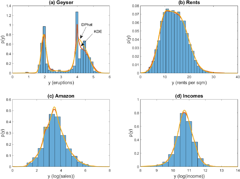
Figure 1: Marginal distributions of the response variables in the four test datasets.

We illustrate our approach using the four real datasets listed in Table 1. Each has one covariate (although we consider multiple covariates in the next section), and we set $x_{i}=w_{i}$ throughout. Fig. 1 plots histograms of the four response variables, along with KDE and Dirichlet process mixture (DPhat) non-parametric density estimates. These are very similar, and we employ the KDE for $F_{Y}$, except where mentioned otherwise. Note that the response in the Geyser dataset in Fig. 1(a) is bimodal, with which most existing distributional regression methods would struggle. In contrast, it is straightforward to account for this feature in our copula approach through the use of a bimodal margin $F_{Y}$. With the Amazon and Incomes datasets, we consider the responses on the logarithmic scale for clarity of illustration, although our regression copula is invariant to monotonic transformations of the response because the copula data $\bm{u}$ is unaffected.

We fit two variants of the copula model. The first employs the copula function $C_{H}$, and is labelled ‘HPSC’ for ‘heteroscedastic P-spline copula’. The second employs $C_{1}$ with the constraint $\text{\boldmath$\alpha$}=\bm{0}$ and is labelled ‘PSC’ for (homoscedastic) ‘P-spline copula’, and is one of the regression copulas proposed by Klein and Smith (2018). Table 2 lists key quantities of the two copulas. Three benchmark models are also considered: the first is labeled PS and is the P-spline smoother with Gaussian errors of Lang and Brezger (2004), the second is labeled ‘HPS’ and is the heteroscedastic P-spline smoother of Klein et al. (2015), while the third is labeled ‘MLT’ and is the ‘most likely transformation’ model of Hothorn et al. (2017). For the latter we use Bernstein polynomials as suggested by the authors, and the method is known to be flexible and robust.

4.1.1 Exact versus approximate estimation

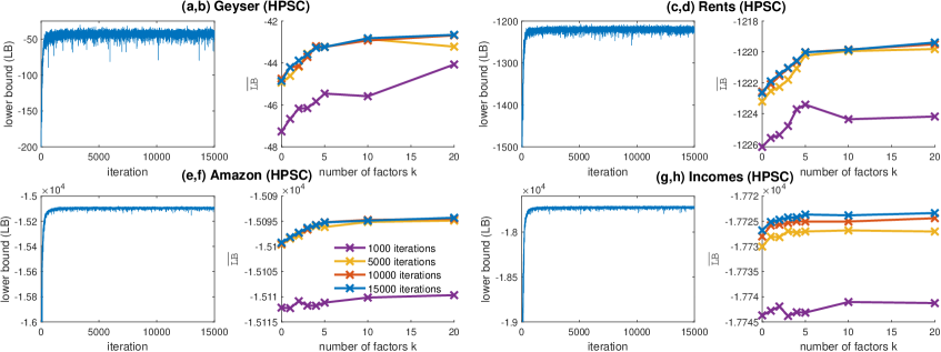
Figure 2: Summaries of the variational lower bound ${\cal L}(\bm{\lambda})$ in the SGA.

We first compare the VB approximate and the HMC exact posterior estimators for the HPSC copula model. The VB estimator was fit using $K=0,1,2,3,4,5,10$ and $20$ factors, and for 1,5,10 and 15 thousand steps. Fig. 2(b,d,f,h) plots the mean lower bound value over the last 10% of steps ($\overline{\mbox{LB}}$) against $K$ for each of the four step sizes and each of the datasets. Increasing $K$ up to 5 improves the accuracy of the VA, but further increases have little impact. Fig. 2(a,c,e,g) plots ${\cal L}(\text{\boldmath$\lambda$})$ against the step number for a VA with $K=20$ factors, and in each case the SGA algorithm converges rapidly. Figs. A and B in the Web Appendix plot the mean and standard deviation of the coefficients $(\text{\boldmath$\beta$},\text{\boldmath$\alpha$})$ from the VA, against their exact posterior means and standard deviations. These show that the variational estimates of the posterior means are highly accurate, but—as is usual in VB inference—the posterior standard deviations are underestimated. Computation times are reported in Table A in the Web Appendix and show that the VB estimator is much faster than the exact method and practical to implement, even for a copula of dimension $n=40,981$.

4.1.2 Predictive accuracy

To compare the accuracy of the five models (PSC, HPSC, PS, HPS and MLT) we compute the predictive logarithmic score by ten-fold cross-validation. For a given dataset, we partition the data into 10 (approximately) equally-sized sub-samples, denoted as $\{(y_{i,k},x_{i,k},w_{i,k});i=1,\ldots,n_{k}\}$ for $k=1,\ldots,10$. For sub-sample $k$, we compute the density estimator using the remaining 9 sub-samples as the training data, and denote these as $\hat{p}_{k}(y|x,w)$. For our copula model we use the density estimator $\hat{p}_{\tiny{PE}}$ in Sec. 3.4. The ten-fold mean logarithmic score is then $\overline{\mbox{LS}}_{CV}=\frac{1}{10}\sum_{k=1}^{10}\frac{1}{n_{k}}\sum_{i=1}^{n_{k}}\log\hat{p}_{k}(y_{i,k}|x_{i,k},w_{i,k})\,.$

Table 3 reports the $\overline{\mbox{LS}}_{CV}$ values, where the posterior of the copulas is computed either exactly using MCMC or HMC, or approximately using VB, with scores given for both cases; we make four observations. First, in all examples both copula models—which account fully for the non-Gaussian distribution of the responses—outperform the two benchmark PS and HPS models. Second, the performance of the copula models estimated using VB is very similar to that of the copula models estimated by exact methods. Third, in every case the HPSC outperforms the PSC, showing that the added flexibility of the heteroscedastic copula translates into improved distributional predictions – something that we demonstrate further below. Last, in all examples HPSC is competitive with the benchmark MLT model, which also allows the entire predictive distribution to vary with the covariates.

4.1.3 Mean and variance function estimates

To compare the distributional regression estimates, Fig. 3 plots the posteriors of $f,v$, computed as in Sec.  3.4 for the Rents dataset. Posterior mean and 95% intervals are given for $f$ in the left-hand panels, and for $v$ in the right-hand panels. Panels (a,b) compare the posteriors from the HPSC model computed exactly using HMC, and approximately using VB, and they are very similar, further illustrating the high accuracy of the VB estimator. Panels (c,d) compare the posteriors from the HPSC model using the three different approaches to estimating $F_{Y}$. These are the kernel estimator (KDE), the Dirichlet process mixture (DPhat), and integrating out $F_{Y}$ using its draws (DP) as in Grazian and Liseo (2017). The posteriors are similar, and the approach used to estimate the margin has little effect on the distributional regression estimates for this example. Panels (e,f) compare the function estimates from the HPSC model against those of the benchmark MLT model, and they differ substantially – particularly for the variance function $v$.

Finally, panels (g,h) compare the function estimates from the two different regression copulas HPSC and PSC. While the estimates of $f$ are similar, those for $v$ are very different. This is because the regression model for the pseudo-response of the PSC is homoscedastic with respect to the covariate, whereas that for the HPSC is heteroscedastic. Fig.C in the Web Appendix plots the posterior estimates of $f,v$ for the other three datasets. Similar results to the Rents dataset are found, where estimates of $f$ from the two regression copula models are similar, but those of $v$ differ substantially.

4.1.4 Dependence metrics and prediction

The improved fit of the HPSC over PSC is because the dependence structure of $C_{H}$ is a much more flexible function of the covariates than $C_{1}$ is with $\text{\boldmath$\alpha$}=\bm{0}$. To illustrate this we construct pairwise dependence metrics as follows. Set $\text{\boldmath$x$}^{+}=\text{\boldmath$w$}^{+}=(\text{\boldmath$x$}^{\prime},x_{n+1},x_{n+2})^{\prime}$, and $\tilde{\text{\boldmath$x$}}^{+}=\{\text{\boldmath$x$}^{+},\text{\boldmath$x$}^{+}\}$, then compute Spearman’s rho for the bivariate sub-copula $C_{H}^{n+1,n+2}$ with $\theta$ integrated out with respect to its posterior; ie:

$$\hat{\rho}^{S}(x_{n+1},x_{n+2})\equiv\int\rho^{S}_{n+1,n+2}(\tilde{\text{\boldmath$x$}}^{+},\text{\boldmath$\theta$})p(\text{\boldmath$\theta$}|\text{\boldmath$y$})\mbox{d}\text{\boldmath$\theta$}\,,$$

where $\rho^{S}_{n+1,n+2}$ is given in Sec. 2.3 part (iii). The integration is computed using draws from the posterior. For the PSC, the coefficients $\bm{\alpha}=\bm{0}$, and integration is only with respect to $\text{\boldmath$\theta$}_{\beta}$. The metric $\hat{\rho}^{S}$ is evaluated on a bivariate grid for $(x_{n+1},x_{n+2})$ over the range of the covariate, and its values plotted as a surface. The process can be replicated for the other dependence metrics.

Fig. N plots the surfaces of $\hat{\rho}^{S}$ for the Rents dataset and both regression copulas. For both copulas, $\hat{\rho}^{S}(x_{n+1},x_{n+2})$ declines as $|x_{n+1}-x_{n+2}|$ increases, which is to be expected from any effective regression smoothing method. However, correlation is locally varying for the HPSC only. For example, correlation is higher for values of the covariate (area) around 20 and 80. Equivalent surfaces for the other three datesets, along with the upper quantile dependence and Kendall’s tau, are given in Part C of the Web Appendix, and the same features can be seen. This local variation in the dependence structure of the HPSC ensures the level of smoothing in the regression and variance functions in Fig. 3 (and Fig.C of the Web Appendix) are ‘locally adaptive’ with respect to the covariate.

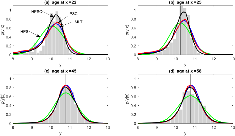
Figure 5: Predictive densities for the Incomes dataset for four different values of age.

In fact, the entire distributional regression fit is locally adaptive to the value of the covariate. To illustrate this, we compute predictive densities for the Incomes dataset from both copula models. Fig. 5 plots these for four values of the covariate (age), along with those from the benchmark HPS and MLT models. Because age is measured discretely, we also provide histograms of the salaries of all individuals of these ages. First, because the HPS model is conditionally Gaussian, the predictive distributions are also, and are inconsistent with the histograms. Second, even though the two copula models share the same margin $F_{Y}$, their predictive densities differ. Those from the HPSC copula model are more consistent with the histograms, which accords with the increased accuracy measured by the scores in Table 3. The MLT densities are similar to those of the PSC copula model, and are also dominated by those from the HPSC copula model.

4.2 Simulation study

We undertake a simulation study to illustrate the efficacy of our copula-based approach to semi-parametric distributional regression. Constructing a simulation design is challenging because all aspects of the distribution are unknown functions of the covariates. Therefore, we base our designs on the five distributional regression methods fitted to the four real datasets in the previous subsection, giving 20 data generating processes (DGPs). From each DGP we simulate 100 datasets (called ‘replicates’ here), and then refit all five methods to every replicate. Accuracy of a method for each fitted replicate is assessed by using it to predict the densities of the observations in an additional 101${}^{\mbox{\small st}}$ replicate. Thus, we are assessing the accuracy of out-of-sample density forecasting. Full details on the simulation study are given in Part D of the Web Appendix.

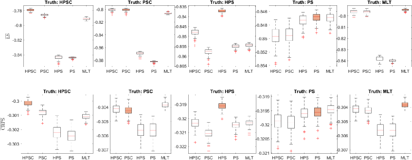
Figure 6: Simulation results for the DGPs constructed from fits to the Incomes dataset.

Fig. 6 gives boxplots of the mean logarithmic score ($\overline{\mbox{LS}}$) and mean continuous ranked probability score ($\overline{\mbox{CRPS}}$) (Gneiting and Raftery, 2007) of predictions for the DGPs based on the Incomes dataset (the other 15 DGPs are given in Part D of the Web Appendix). The shaded boxplots are for the method that matches the DGP in each panel, and these are (unsurprisingly) either the best, or equal best, at recapturing the DGP. Our focus is therefore on the next best performers, and we make three observations. First, when the DGP is either copula model, the HPSC either equals or out-performs the PSC, highlighting its superiority as a regression copula. Second, when the DGP is the HPS, then the regression copula HPSC is best at recapturing this DGP. Last, the HPSC either equals or out-performs the MLT benchmark method for all DGPs and metrics, except for the PS DGP. Results for the other 15 DGPs are similar.

5 Radial Basis Copula for Electricity Prices

The relationship between intra-day electricity spot price and demand is used by participants in wholesale markets to formulate optimal bidding strategies (Kirschen and Strbac, 2004, pp.53–72). However, its estimation using regression methods is difficult because prices have a very heavy right tail, and all aspects of their distribution vary extensively with demand, day and time of day (Bunn et al., 2016). To account for this, we construct a regression copula from trivariate radial bases for $\tilde{m},g$, combined with horseshoe priors for regularization. We apply it to high-frequency Australian electricity price and demand data, and compare our approach to other distributional regression methods.

5.1 Electricity data and regression copula model

The Australian national electricity market (NEM) is a wholesale market where generators, distributors and third party participants bid for the sale and purchase of electricity one day ahead of transmission; see Ignatieva and Trück (2016) and Smith and Shively (2018) for current descriptions of the market. We consider half-hourly market-wide price $P_{i}$ and total market demand $D_{i}$ from 1 Jan 2014 to 31 Dec 2018, so that $n=87,648$. Total market demand is the sum of demand across the five regions in the NEM, while the market-wide price is the demand-weighted average price across the five regions, constructed from data available at www.aemo.com.au. The three covariates are demand, time of day ($\mbox{TOD}_{i}$) and day number ($\mbox{Day}_{i}$), and set $\text{\boldmath$x$}_{i}=\text{\boldmath$w$}_{i}=(D_{i},\mbox{TOD}_{i},\mbox{Day}_{i})^{\prime}$, with each covariate scaled to the unit interval. For $\tilde{m}$ and $g$ we employ thin plate spline radial basis functions (RBF) of the form $b_{j}(\text{\boldmath$x$})=\delta(\text{\boldmath$x$}-\text{\boldmath$k$}_{j})^{2}\log(\delta(\text{\boldmath$x$}-\text{\boldmath$k$}_{j}))$ for knot $\text{\boldmath$k$}_{j}$. The distance function $\delta(x_{1},x_{2},x_{3})=||(x_{1},\sin(\pi x_{2}),x_{3})||$ is the Euclidean distance with a sine transformation on the second element to ensure the basis is periodic on $[0,1)$ for $\mbox{TOD}_{i}$. The knots are set equal to a random sample (stratified by time of day) of 240 and 96 covariate values for $\tilde{m}$ and $g$, respectively. We follow Klein and Smith (2018) and use the horseshoe prior for the regularization at Eq. (6), and provide details in Part E of the Web Appendix.

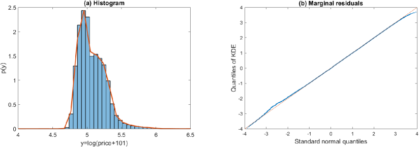
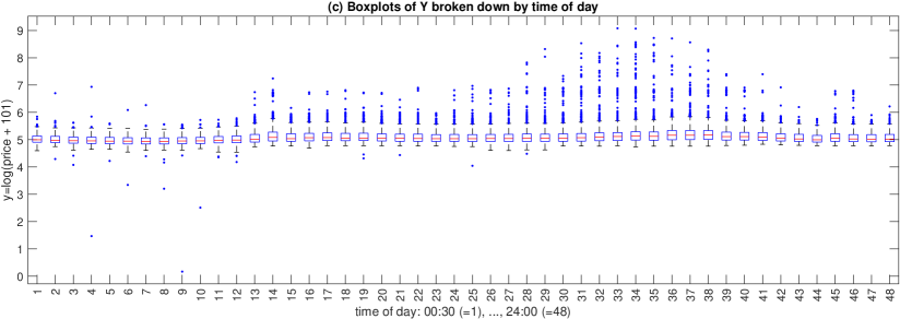
Figure 7: Marginal distribution summaries of the logarithm of half-hourly electricity prices.

Due to the extreme skew in electricity prices we set $Y_{i}=\log(P_{i}+101)$, where we add 101 before taking the logarithm because the minimum observed price in our data is $-\$99.82$ (prices can be negative in the NEM). Fig. 7(a) plots a histogram of the response and KDE $\hat{F}_{Y}$, showing that even on the logarithmic scale the distribution of prices is positively skewed and heavy-tailed. Panel (b) gives a quantile-quantile plot highlighting the accuracy of the KDE estimator for $F_{Y}$. Panel (c) contains boxplots of the response broken down by the time of day, and reveals the strong diurnal variation in the entire distribution of prices.

5.2 Empirical results

We estimate our regression copula (labeled ‘HRBFC’) using VB with $K=20$ factors for the approximation. A plot of ${\cal L}(\text{\boldmath$\lambda$})$ against step number (see Web Appendix) indicates reliable convergence of the SGA algorithm. There is a strong (non-additive) effect of the three covariates on price. For example, Fig. 8 plots a ‘slice’ of the trivariate mean $f$ and variance $v$ functions against demand $D_{i}$ for 12 May 2018 at 19:00, which is the time of day with the highest mean price. They are the variational posteriors, computed as at Eq. (16), and show the positive relationship between the first two moments of price and demand.

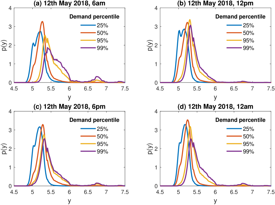
Figure 10: Predictive distributions of the logarithm of electricity prices from the regression copula model (HRBFC).

To illustrate the impact of demand on the entire distribution, Fig. 10 plots the predictive densities of $Y$ on 12 May 2018 at (a) 06:00, (b) 12:00, (c) 18:00 and (d) 24:00. In each panel, densities are constructed at four levels of demand that correspond to the 0.25, 0.5, 0.95 and 0.99 percentiles of demand at each time of day. Increases in demand accentuate the upper tail, consistent with the nonlinear impact of demand shocks on price spikes documented previously (Higgs and Worthington, 2008; Smith and Shively, 2018). Further plots of predictive densities over the four years (see Part F of the Web Appendix) show the upper tail is increasingly sensitive to demand, matching the increasing frequency of price spikes during the period.

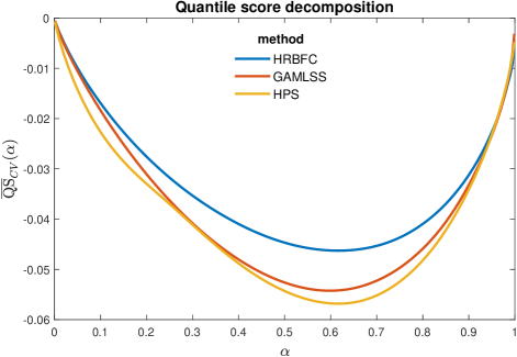
Figure 9: Mean quantile score for the electricity price example.

Last, we compare our regression copula to two benchmarks models. The first is the approach of Rigby and Stasinopoulos (2005) (labeled ‘GAMLSS’) where we tried several distributions and found the ST2 to give the best fit. We found convergence problems when specifying all parameters as additive splines of the three covariates, and were restricted to only allow the mean and variance to do so. The second benchmark is a heteroscedastic regression model with additive P-spline terms for the three covariates (labeled ‘HPS’). To measure the accuracy of the distributional forecasts for the three models, Table 4 reports the cross-validated mean score metric $\overline{\mbox{LS}}_{CV}$ defined in Sec. 4.1.2, plus a 10-fold cross-validated mean CRPS metric ($\overline{\mbox{CRPS}}_{CV}$). The radial basis regression copula model clearly dominates the GAMLSS and HPS benchmarks. Fig. 9 plots the (cross-validated) mean quantile score $\overline{QS}_{CV}(\alpha)=\frac{1}{10}\sum_{k=1}^{10}\frac{1}{n_{k}}\sum_{i=1}^{n_{k}}\widehat{\mbox{QS}}_{k}(y_{i,k};\alpha|x_{i,k},w_{i,k})$ for each method and $\alpha\in(0,1)$, where $\widehat{\mbox{QS}}_{k}(y;\alpha|\text{\boldmath$x$},\text{\boldmath$w$})\equiv-\mbox{QS}_{\alpha}(\hat{F}_{k}^{-1}(\alpha),y)$ is defined in Gneiting and Ranjan (2011). All scores are orientated so that higher values indicate greater accuracy. The figure reveals the greater accuracy of the HRBFC model at all quantiles, except for the extreme tails where the three models are similar. Predictive density forecasts from GAMLSS and HPS are provided in Part F of the Web Appendix, and show they (unlike those from the HRBFC model) are only weakly effected by increases in demand, which is inconsistent with previous analyses (Higgs and Worthington, 2008; Ignatieva and Trück, 2016; Smith and Shively, 2018).

6 Discussion

This paper proposes modeling the entire distribution of a vector of regression response values, conditional on covariates, using a copula decomposition. To do so, a new copula $C_{H}$ is constructed from a heteroscedastic semi-parametric regression for a pseudo-response. When combined with non-parametric or other margins, the resulting regression model is flexible in both the distributional shape and the functional relationship between the covariates and response. Our approach is very general, scalable and numerically stable. We show in our empirical work that it improves predictive accuracy for non-Gaussian data, relative to a number of leading benchmark regression approaches.

A number of authors construct the $n$-dimensional implicit Gaussian copulas of Gaussian processes (Wauthier and Jordan, 2010; Wilson and Ghahramani, 2010). However, these are very different copulas than those constructed here. Klein and Smith (2018) propose constructing the copula of Bayesian regularized smoothers, which is equivalent to our implicit copula when $\text{\boldmath$\alpha$}=\bm{0}$. This paper extends their work by allowing for heteroscedasticity in the pseudo-response, which yields a copula with a much richer dependence structure as shown in Fig. N. This makes the distributional regression locally adaptive, as can be seen in the mean and variance function estimates in Fig. 3, and increases predictive accuracy. However, our proposed copula is more difficult to estimate, and the MCMC schemes discussed by Klein and Smith (2018)—who do not consider alternatives—are infeasible. To address this, we develop efficient exact estimation with a HMC step for generating $\alpha$, and approximate estimation using VB. The empirical work demonstrates the efficacy these methods using five diverse real datasets. In every case, our fitted copula model is more accurate than both the simpler regression copula $C_{1}$ with $\text{\boldmath$\alpha$}=\bm{0}$ and the benchmark models. Moreover, estimation and prediction is fast, allowing the application of the distributional regression methodology to large datasets.

Table 1: Details and source of the four univariate datasets.

Dataset	$n$	Covariate	Response	Source
Geyser	299	waiting time (min)	eruption time (min)	Venables and Ripley (2002)
Rents	3,082	apartment area (m2)	residential rent (EUR/m2)	Fahrmeir et al. (2013)
Amazon	31,925	website visit duration (min)	$\log$(sales) ($\log(\mbox{USD})$)	Panagiotelis et al. (2014)
Incomes	40,981	worker age (years)	$\log$(income) (EUR)	Klein et al. (2015)

The columns give (in order) the dataset name, number of observations, covariate, response variable, and published source of the data.

Table 2: Key quantities of the two P-spline regression copulas PSC and HPSC.

Quantity	PSC	HPSC
$\vartheta$	$\text{\boldmath$\vartheta$}=\{\text{\boldmath$\beta$},\text{\boldmath$\theta$}_{\beta}\}$	$\text{\boldmath$\vartheta$}=\{\text{\boldmath$\beta$},\text{\boldmath$\alpha$},\text{\boldmath$\theta$}_{\beta},\text{\boldmath$\theta$}_{\alpha}\}$
$s_{i}$	$s_{i}=(1+\text{\boldmath$b$}_{i}^{\prime}P_{\beta}(\text{\boldmath$\theta$}_{\beta}^{-1})\text{\boldmath$b$}_{i})^{-1/2}$	$s_{i}=(\exp(\text{\boldmath$v$}_{i}^{\prime}\text{\boldmath$\alpha$})+\text{\boldmath$b$}_{i}^{\prime}P_{\beta}(\text{\boldmath$\theta$}_{\beta}^{-1})\text{\boldmath$b$}_{i})^{-1/2}$
$S$	$S(\text{\boldmath$x$},\text{\boldmath$\theta$}_{\beta})$	$S(\text{\boldmath$x$},\text{\boldmath$w$},\text{\boldmath$\alpha$},\text{\boldmath$\theta$}_{\beta})$
$R$	$R(\text{\boldmath$x$},\text{\boldmath$\theta$}_{\beta})=S(I+BP_{\beta}(\text{\boldmath$\theta$}_{\beta}^{-1})B^{\prime})S^{\prime}$	$R(\tilde{\text{\boldmath$x$}},\text{\boldmath$\alpha$},\text{\boldmath$\theta$}_{\beta})=S(\exp(V\text{\boldmath$\alpha$})+BP_{\beta}(\text{\boldmath$\theta$}_{\beta}^{-1})B^{\prime})S^{\prime}$

Reported from the top to bottom rows are: augmented parameters, normalizing factor, normalizing matrix, and parameter matrix of the Gaussian copula $C_{1}$.

Table 3: Predictive accuracy of distributional regression methods for four test datasets.

	Model / Estimation Method
	PSC/		HPSC/		PS/	HPS/	MLT/
Dataset	VB	MCMC	VB	HMC	MCMC	MCMC	MLE
Geyser	-189.80	-190.08	-187.52	-188.19	-409.86	-349.56	-259.38
Rents	-89,105	-89,015	-88,949	-88,959	-89,285	-89,277	-88,973
Amazon	-42,328	-42,253	-42,207	-42,213	-43,064	-42,898	-42,409
Incomes	-33,339	-32,722	-32,396	-32.530	-35,259	-35,102	-32,840

The 10-fold cross-validated mean predictive logarithmic scores ($\overline{\mbox{LS}}_{CV}$) multiplied by $n$ for presentation. Higher values indicate greater accuracy. The models are the two regression copula models (PSC and HPSC), and the benchmark Gaussian P-spline (PS), its heteroscedastic version (HPS) and the ‘most likely transformation’ method (MLT). The Bayesian posterior of the copulas are computed either exactly using MCMC or HMC, or approximately using VB, with scores given for both cases.

Table 4: Two measures of predictive accuracy for the Australian electricty spot price data.

Metric	HRBFC	HPS	GAMLSS
$\overline{\mbox{LS}}_{CV}$	0.8416	0.4351	0.6926
$\overline{\mbox{CRPS}}_{CV}$	-0.0677	-0.0809	-0.0772

The 10-fold cross-validated mean predictive logarithmic score ($\overline{\mbox{LS}}_{CV}$) and continuous ranked probability score ($\overline{\mbox{CRPS}}_{CV}$), for density forecasts from the three distributional regressions. Higher values indicate greater predictive accuracy. The models are the radial basis regression copula (HRBFC), heteroscedastic P-spline (HPS) and GAMLSS with family ST2.

Normalized histograms of the response ($Y$) of the four datasets in Section 4, along with kernel (KDE) and Bayesian (DPhat) non-parametric density estimates of $p_{Y}$. The datasets are (a) Geyser, (b) Rents, (c) Amazon and (d) Incomes.

The datasets are (a,b) Geyser, (c,d) Rents, (e,f) Amazon, and (g,h) Incomes. Panels (b,d,f,h) plot the average lower bound ($\overline{\mbox{LB}}$) over the last 10% of steps, against the number of factors $K$ in the Gaussian factor variational approximation. Panels (a,c,e,g) plot the variational lower bound against step number for the approximation with $K=20$ factors.

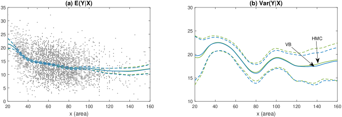
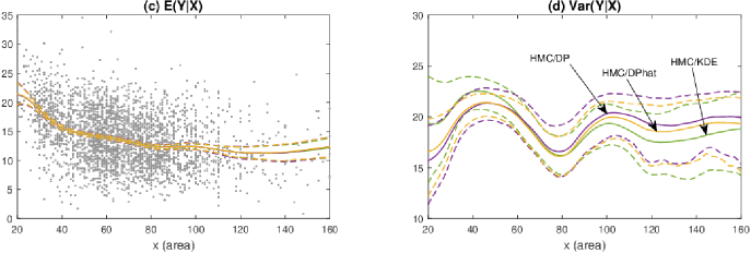
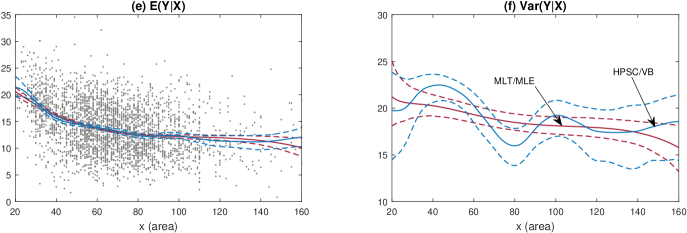
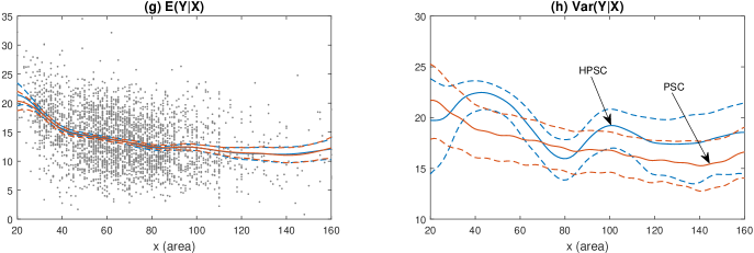
Figure 3: Comparison of different posterior estimates of the regression function $f$ (left-hand side) and variance function $v$ (right-hand side) for the Rents data.

The posterior means of $f$ and $v$ are given as solid lines, and 95% posterior intervals by dashed lines. Scatterplots of the data are included on the left-hand panels. Panels (a,b) compare function estimates from the HPSC model computed using HMC and VB. Panels (c,d) compare function estimates computed using HMC from the HPSC model using three different marginal estimators discussed in the text: KDE, DPhat and DP. Panels (e,f) compare function estimates from the HPSC model (computed using HMC) with those from the benchmark MLT model. Panels (g,h) show estimates of the regression function $f$ (left-hand side) and variance function $v$ (right-hand side) from the HPSC model, compared to those from the PSC model.

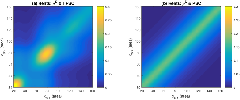
Figure 4: Spearman’s rho from the regression copulas for the Rents dataset.

Each panel plots estimates of Spearman’s rho $\hat{\rho}^{S}(x_{n+1},x_{n+2})$ as bivariate functions of $(x_{n+1},x_{n+2})$ over the range of the covariate (area). Panel (a) gives values for the HPSC, and panel (b) for the PSC. The localized variation in $\hat{\rho}^{S}$ in panel (a) corresponds to local adaptivity in the distributional regression from the copula model. Analogous plots for the other three datasets, and other dependence metrics (Kendall’s tau, upper and lower quantile dependence) are given in the Web Appendix.

The different ages are (a) 22 years old, (b) 24 years old, (c) 45 years old, and (d) 58 years old. Densities are from the PSC (red), HPSC (black), HPS (green) and MLT (blue) regression models. Also plotted are histograms of the sub-samples of individuals with these four ages in the Incomes dataset.

The top panels report the mean logarithmic score ($\overline{\mbox{LS}}$), and the bottom panels the mean CRPS ($\overline{\mbox{CRPS}}$). These are out-of-sample density forecasting metrics averaged over observations in a 101st replicate. Results are orientated so that higher values correspond to greater accuracy. The columns give results for replicates simulated from each of the DGPs obtained from fitting the five distributional regression models to the original data. In each panel boxplots of the metrics for each the 100 replicates are given, with one boxplot for each of the five methods. The shaded boxplots are for the cases where the method matches the DGP used to generate the data, which will typically be most accurate.

Summaries are for $Y=\log(\mbox{Price}+101)$. Panel (a) plots a histogram and the KDE $\hat{F}_{Y}$ over the range $4<Y<6.5$, although the tails of the marginal distribution extend further. Panel (b) provides a quantile-quantile plot of the residuals from the marginal fit $\hat{F}_{Y}$. Panel (c) provides boxplots of $Y$ broken down by time of day, revealing the diurnal variation in the distribution.

Figure 8: The mean and variance of the logarithm of price as a function of demand from the regression copula model.

Panel (a) plots the mean function $f$ and panel (b) the variance function $v$ against demand (in GW/h) for 12 May 2018 at 19:00 (the peak demand time of day). The (variational) posterior mean estimates of the functions are given in bold, while the approximate 95% posterior intervals are given in dashed lines.

The 10-fold cross-validated mean quantile score function ($\overline{\mbox{QS}}_{CV}(\alpha)$) orientated so that higher values correspond to greater accuracy, and plotted against quantile $0<\alpha<1$ for the regression copula model (HRBFC), and GAMLSS, HPS benchmarks.

The four panels provide predictions for 12 May 2018 at (a) 06:00, (b) 12:00, (c) 18:00 and (d) 24:00. In each panel, the predictive densities are constructed at four levels of demand corresponding to the 0.25, 0.5, 0.95 and 0.99 percentiles of demand at each time of day.

Web Appendix for
‘Bayesian Inference for Regression Copulas’

Contents

• Part A: Proofs and derivations.

• Part B: Derivation of the derivatives required to implement the exact and approximate inferential schemes for the HPSC and PSC in Section 4, and pseudo code for the exact sampler of Section 3.

• Part C: Additional figures and tables referred to in Section 4.1 of the manuscript.

• Part D: Details and additional figures on the simulation in Section 4.2 of the manuscript and additional results.

• Part E: Details and derivatives required to implement the approximate inferential scheme for the HRBFC in Section 5.

• Part F: Additional figures referred to in Section 5 of the manuscript.

Appendix Part A Proofs and Derivations

Part A.1 Margin of $Y_{i}$

Regression models are usually specified conditional on parameters for the mean, variance and possibly other moments. In contrast, the definition of the regression copula model at Eq. (1) is unconditional on such parameters, and the margin $F_{Y}$ of $Y_{i}$ is assumed to be invariant with respect to the covariates $\tilde{\text{\boldmath$x$}}_{i}$. However, $Y_{i}$ is dependent on $\tilde{\text{\boldmath$x$}}_{i}$ when also conditioning on the mean and variance functions $\tilde{m},g$ of the pseudo-response, as we now show. First, from Eq. (8) the normalized response has distribution $Z_{i}|\tilde{\text{\boldmath$x$}}_{i},\tilde{m},g\sim N(m(\text{\boldmath$x$}_{i},\text{\boldmath$w$}_{i}),s_{i}^{2}\sigma_{i}^{2})$. From Theorem 1, $U_{i}=\Phi_{1}(Z_{i})$, so that $Y_{i}=F_{Y}^{-1}(\Phi_{1}(Z_{i}))$, and the Jacobean of the transformation is $p_{Y}(y_{i})/\phi_{1}(z_{i})$. Then the density of the conditional distribution is:

$$p(y_{i}|\tilde{\text{\boldmath$x$}}_{i},\tilde{m},g)=p(z_{i}|\tilde{\text{\boldmath$x$}}_{i},\tilde{m},g)\frac{p_{Y}(y_{i})}{\phi_{1}(z_{i})}=\frac{1}{s_{i}\sigma_{i}}\phi_{1}\left(\frac{z_{i}-m(\text{\boldmath$x$}_{i},\text{\boldmath$w$}_{i})}{s_{i}\sigma_{i}}\right)\frac{p_{Y}(y_{i})}{\phi_{1}(z_{i})}\,.$$

Thus, the distribution of $Y_{i}$ is a function of $\tilde{\text{\boldmath$x$}}_{i}=\{\text{\boldmath$x$}_{i},\text{\boldmath$w$}_{i}\}$ when also conditioning on $\tilde{m},g$.

Part A.2 Proof of Theorem 1

Recall that $\tilde{\text{\boldmath$x$}}=\{\text{\boldmath$x$},\text{\boldmath$w$}\}$ and $\text{\boldmath$\theta$}=\{\text{\boldmath$\theta$}_{\alpha},\text{\boldmath$\theta$}_{\beta}\}$, and note that the distribution $Z_{i}|\tilde{\text{\boldmath$x$}},\text{\boldmath$\theta$}$ is standard normal because

$$p(z_{i}|\tilde{\text{\boldmath$x$}},\text{\boldmath$\theta$}) =\int p_{Z_{i}}(z_{i}|\tilde{\text{\boldmath$x$}},\text{\boldmath$\alpha$},\text{\boldmath$\theta$}_{\beta})\,p(\text{\boldmath$\alpha$}|\text{\boldmath$\theta$}_{\alpha})\mathrm{d}\text{\boldmath$\alpha$}=\int\phi_{1}(z_{i})\,p(\text{\boldmath$\alpha$}|\text{\boldmath$\theta$}_{\alpha})\mathrm{d}\text{\boldmath$\alpha$}=\phi_{1}(z_{i})\,,$$

while $p_{Z}(\text{\boldmath$z$}|\tilde{\text{\boldmath$x$}},\text{\boldmath$\alpha$},\text{\boldmath$\theta$}_{\beta})=c_{1}(\text{\boldmath$u$}|\bm{x},\bm{w},\text{\boldmath$\alpha$},\text{\boldmath$\theta$}_{\beta})\prod_{i=1}^{n}\phi_{1}(z_{i})$. Then, the implicit copula density (Nelsen, 2006, Sec 3.1) of $\bm{Z}|\tilde{\text{\boldmath$x$}},\text{\boldmath$\theta$}$ is given by

$$c_{H}(\text{\boldmath$u$}|\tilde{\text{\boldmath$x$}},\text{\boldmath$\theta$}) =\frac{p(\text{\boldmath$z$}|\tilde{\text{\boldmath$x$}},\text{\boldmath$\theta$})}{\prod_{i=1}^{n}\phi_{1}(z_{i})}=\frac{\int p_{Z}(\text{\boldmath$z$}|\tilde{\text{\boldmath$x$}},\text{\boldmath$\alpha$},\text{\boldmath$\theta$}_{\beta})\,p(\text{\boldmath$\alpha$}|\text{\boldmath$\theta$}_{\alpha})\mathrm{d}\text{\boldmath$\alpha$}}{\prod_{i=1}^{n}\phi_{1}(z_{i})}$$

$$=\frac{\int c_{1}(\text{\boldmath$u$}|\bm{x},\bm{w},\text{\boldmath$\alpha$},\text{\boldmath$\theta$}_{\beta})\prod_{i=1}^{n}\phi_{1}(z_{i})p(\text{\boldmath$\alpha$}|\text{\boldmath$\theta$}_{\alpha})\mathrm{d}\text{\boldmath$\alpha$}}{\prod_{i=1}^{n}\phi_{1}(z_{i})}=\int c_{1}(\text{\boldmath$u$}|\bm{x},\bm{w},\text{\boldmath$\alpha$},\text{\boldmath$\theta$}_{\beta})p(\text{\boldmath$\alpha$}|\text{\boldmath$\theta$}_{\alpha})\mathrm{d}\text{\boldmath$\alpha$}\,,$$

which is the required expression for $c_{H}$ in Theorem 1. Similarly, if $F_{Z}(\text{\boldmath$u$}|\tilde{\text{\boldmath$x$}},\text{\boldmath$\theta$})$ denotes the joint distribution function of $\bm{Z}|\tilde{\text{\boldmath$x$}},\text{\boldmath$\theta$}$, then its implicit copula function (Nelsen, 2006, Sec.3.1) is

$$C_{H}(\text{\boldmath$u$}|\tilde{\text{\boldmath$x$}},\text{\boldmath$\theta$}) = F(\text{\boldmath$z$}|\tilde{\text{\boldmath$x$}},\text{\boldmath$\theta$})=\int\int p_{Z}(\text{\boldmath$z$}|\tilde{\text{\boldmath$x$}},\text{\boldmath$\alpha$},\text{\boldmath$\theta$}_{\beta})p(\text{\boldmath$\alpha$}|\text{\boldmath$\theta$}_{\alpha})\mbox{d}\text{\boldmath$\alpha$}\mbox{d}\text{\boldmath$z$}$$

$$= \int\int\phi(\text{\boldmath$z$};\bm{0},R)\mbox{d}\text{\boldmath$z$}\,p(\text{\boldmath$\alpha$}|\text{\boldmath$\theta$}_{\alpha})\mbox{d}\text{\boldmath$\alpha$}=\int\Phi(\text{\boldmath$z$};\bm{0},R)p(\text{\boldmath$\alpha$}|\text{\boldmath$\theta$}_{\alpha})\mbox{d}\text{\boldmath$\alpha$}$$

$$= \int C_{1}(\text{\boldmath$u$}|\text{\boldmath$x$},\text{\boldmath$w$},\text{\boldmath$\alpha$},\text{\boldmath$\theta$}_{\beta})p(\text{\boldmath$\alpha$}|\text{\boldmath$\theta$}_{\alpha})\mbox{d}\text{\boldmath$\alpha$}\,.$$

Part A.3 Proof of Theorem 2

First, note that $|C_{1}(\text{\boldmath$u$}|\text{\boldmath$x$},\text{\boldmath$w$},\text{\boldmath$\alpha$},\text{\boldmath$\theta$}_{\beta})\,p(\text{\boldmath$\alpha$}|\text{\boldmath$\theta$}_{\alpha})|\leq M(\text{\boldmath$u$})\,p(\text{\boldmath$\alpha$}|\text{\boldmath$\theta$}_{\alpha})$, where $M(\text{\boldmath$u$})$ is the upper Fréchet-Hoeffding bound. Also note that from the definition of $R$,

$$\lim\limits_{\gamma_{\beta}\rightarrow 0}R=S^{\star}\Sigma S^{\star}=I_{n}\,,$$

where $S^{\star}=\mbox{diag}(\exp(-\text{\boldmath$v$}_{1}^{\prime}\text{\boldmath$\alpha$}/2),\ldots,\exp(-\text{\boldmath$v$}_{n}^{\prime}\text{\boldmath$\alpha$}/2))$ . Then, by Theorem 1 and Lebesgue’s dominated convergence theorem,

$$\lim\limits_{\gamma_{\beta}\rightarrow 0}C_{H}(\text{\boldmath$u$}|\tilde{\text{\boldmath$x$}},\text{\boldmath$\theta$}) = \int\lim\limits_{\gamma_{\beta}\rightarrow 0}C_{1}(\text{\boldmath$u$}|\text{\boldmath$x$},\text{\boldmath$w$},\text{\boldmath$\theta$}_{\beta},\text{\boldmath$\alpha$})\,p(\text{\boldmath$\alpha$}|\text{\boldmath$\theta$}_{\alpha})\mbox{d}\text{\boldmath$\alpha$}$$

$$= \int\lim\limits_{\gamma_{\beta}\rightarrow 0}\Phi(\text{\boldmath$z$};\bm{0},R)\,p(\text{\boldmath$\alpha$}|\text{\boldmath$\theta$}_{\alpha})\mbox{d}\text{\boldmath$\alpha$}=\int\Phi(\text{\boldmath$z$};\bm{0},I)\,p(\text{\boldmath$\alpha$}|\text{\boldmath$\theta$}_{\alpha})\mbox{d}\text{\boldmath$\alpha$}$$

$$= \Phi(\text{\boldmath$z$};\bm{0},I)=\Phi((\Phi_{1}^{-1}(u_{1}),...,\Phi_{1}^{-1}(u_{n}))^{\prime};0,I)$$

$$= \prod_{i=1}^{n}\Phi_{1}(\Phi_{1}^{-1}(u_{i}))=\Pi(\text{\boldmath$u$})\,.$$

Part A.4 Derivation of Dependence Metrics for $C_{H}^{ij}$

To derive the lower quantile dependence metric at part (i),

$$\lambda^{L}_{ij}(q|\tilde{\text{\boldmath$x$}},\text{\boldmath$\theta$}) = \frac{C_{H}^{ij}(q,q)}{q}=\int\frac{C_{1}^{ij}(q,q)\,p(\text{\boldmath$\alpha$}|\text{\boldmath$\theta$}_{\alpha})}{q}\mbox{d}\text{\boldmath$\alpha$}=\int\lambda^{L}_{1}(q|\text{\boldmath$x$},\text{\boldmath$w$},\text{\boldmath$\alpha$},\text{\boldmath$\theta$}_{\beta})\,p(\text{\boldmath$\alpha$}|\text{\boldmath$\theta$}_{\alpha})\mbox{d}\text{\boldmath$\alpha$}\,.$$

The derivation of the upper quantile dependence is similar.

To derive the metrics at part (ii), first note that for any bivariate copula function $C$, if $M(u,v)=\min(u,v)$ is the upper Fréchet-Hoeffding bound, then $|C(q,q)/q|\leq M(q,q)/q=1$. Denote the $(i,j)$th element of $R$ as $r_{ij}$, and the sub-copulas of $C_{1}$ and $C_{H}$ in these elements as $C_{1}^{ij}$ and $C_{H}^{ij}$. Then, by Theorem 1 and Lebesgue’s dominated convergence theorem,

$$\lambda^{L}_{ij}=\lim\limits_{q\downarrow 0}\frac{C_{H}^{ij}(q,q)}{q}=\int\lim\limits_{q\downarrow 0}\frac{C_{1}^{ij}(q,q)}{q}p(\text{\boldmath$\alpha$}|\text{\boldmath$\theta$}_{\alpha})\mbox{d}\text{\boldmath$\alpha$}=0$$

because $C_{1}^{ij}$ is a Gaussian copula with zero tail dependence, so that $\lim\limits_{q\downarrow 0}\frac{C_{1}^{ij}(q,q)}{q}=0$. The derivation of $\lambda^{U}$ is similar.

The derivation of $\rho^{S}_{ij}$ in part (iii) follows from the definition of Spearman’s correlation, and its expression for a Gaussian copula, as follows:

$$\rho^{S}_{ij}(\tilde{\text{\boldmath$x$}},\text{\boldmath$\theta$}) = 12\int C_{H}^{ij}(u,v)\mbox{d}(u,v)-3=12\int\int C_{1}^{ij}(u,v)\,p(\text{\boldmath$\alpha$}|\text{\boldmath$\theta$}_{\alpha})\mbox{d}(u,v)\mbox{d}\text{\boldmath$\alpha$}-3$$

$$= \int\left(12\int C_{1}^{ij}(u,v)\mbox{d}(u,v)-3+3\right)\,p(\text{\boldmath$\alpha$}|\text{\boldmath$\theta$}_{\alpha})\mbox{d}\text{\boldmath$\alpha$}-3$$

$$= \frac{6}{\pi}\int\arcsin(r_{ij}/2)\,p(\text{\boldmath$\alpha$}|\text{\boldmath$\theta$}_{\alpha})\mbox{d}\text{\boldmath$\alpha$}\,.$$

The derivation of $\tau^{K}_{ij}$ is similar.

Appendix Part B Details on Estimation

Part B.1 Exact Estimation

We now review the implemented steps for exact inference for the HPSC. Recall that for this copula $\text{\boldmath$\theta$}_{\beta}=\{\tau^{2}_{\beta},\psi_{\beta,1},\psi_{\beta,2}\}$ and $\text{\boldmath$\theta$}_{\alpha}=\{\tau^{2}_{\alpha},\psi_{\alpha,1},\psi_{\alpha,2}\}$, and the precision matrices can be factorized as $P_{\beta}(\text{\boldmath$\theta$}_{\beta})=\frac{1}{\tau^{2}_{\beta}}P(\text{\boldmath$\psi$}_{\beta})$ and $P_{\alpha}(\text{\boldmath$\theta$}_{\alpha})=\frac{1}{\tau^{2}_{\alpha}}P(\text{\boldmath$\psi$}_{\alpha})$, where $P(\text{\boldmath$\psi$})$ is the usual band two scaled precision matrix of an AR(2) process with partial autoregressive coefficients $\psi$. The complete algorithm is provided at the end of this Section in Algorithm 3. The sampler for the PSC is obtained by simply skipping the generation steps of $\alpha$ and $\text{\boldmath$\theta$}_{\alpha}.$

Part B.1.1 Gibbs update for $\beta$

We generate from the conditional posterior $p(\text{\boldmath$\beta$}|\text{\boldmath$x$},\text{\boldmath$w$},\text{\boldmath$y$},\{\text{\boldmath$\theta$}\setminus\text{\boldmath$\beta$}\})=p(\text{\boldmath$\beta$}|\text{\boldmath$x$},\text{\boldmath$z$},\{\text{\boldmath$\theta$}\setminus\text{\boldmath$\beta$}\})$ which is Gaussian with mean $\text{\boldmath$\mu$}_{\beta}=\Sigma_{\beta}B^{\prime}\Sigma^{-1}S^{-1}\text{\boldmath$z$}$ and covariance matrix $\Sigma_{\beta}=(B^{\prime}\Sigma^{-1}B+P_{\beta}(\text{\boldmath$\theta$}_{\beta}))^{-1}$.

Part B.1.2 MH step for $\text{\boldmath$\theta$}_{\beta}$

We generate each element of $\text{\boldmath$\theta$}_{\beta}$ separately, relying on analytical derivatives for the proposal densities and by making the algorithm extremely efficient as we only store the unique rows of the design matrices $B$.

A Metropolis-Hastings step is used to generate $\tilde{\tau}_{\beta}^{2}=\log(\tau_{\beta}^{2})$, where a normal distribution matching the mode and curvature is used to approximate its conditional. Note that

$$l_{{\tilde{\tau}_{\beta}^{2}}}\equiv\log(p({\tilde{\tau}_{\beta}^{2}}|\text{\boldmath$x$},\text{\boldmath$w$},\text{\boldmath$y$},\{\text{\boldmath$\theta$}\setminus\tau_{\beta}^{2}\}))\propto-\frac{{\tilde{\tau}_{\beta}^{2}}}{2}\left(p_{1}-1\right)-\frac{1}{2\exp({\tilde{\tau}_{\beta}^{2}})}\text{\boldmath$\beta$}^{\prime}P(\text{\boldmath$\psi$}_{\beta})\text{\boldmath$\beta$}-\left(\frac{\exp({\tilde{\tau}_{\beta}^{2}})}{b_{\tau_{\beta}^{2}}}\right)^{\tfrac{1}{2}}$$

$$\quad\quad\quad\qquad\qquad\qquad\quad\;\,-\frac{1}{2}\sum_{i=1}^{n}\log(s_{i}^{2})-\frac{1}{2}\left(\text{\boldmath$z$}^{\prime}(S\Sigma S^{\prime})^{-1}\text{\boldmath$z$}-2\text{\boldmath$\beta$}^{\prime}B^{\prime}\Sigma^{-1}S^{-1}\text{\boldmath$z$}\right).$$

Approximating $l_{{\tilde{\tau}_{\beta}^{2}}}$ by a second order Taylor expansion around the current state ${{\tilde{\tau_{\beta}^{2}}}}^{(m)}$, and taking the exponent yields a Gaussian proposal density involving the score function and the second derivative of the conditional posterior above. Analytical expressions for these are given in Appendix B.1 of Klein and Smith (2018) after replacing $P((\psi_{\beta,1},\psi_{\beta,2})^{\prime})$ by $P(\psi_{\beta})$, $S^{2}$ by $S\Sigma S^{\prime}$, and $\text{\boldmath$\beta$}^{\prime}B^{\prime}\Sigma^{-1}S^{-1}\text{\boldmath$z$}$ by $\text{\boldmath$\beta$}^{\prime}B^{\prime}S^{-1}\text{\boldmath$z$}$.

To improve sampling behaviour, we transform $\psi_{\beta,j}\in[-1+\epsilon,1-\epsilon]$ component-wise for $j=1,2$ onto the real line via $\tilde{g}:[-1+\epsilon,1-\epsilon]\to\text{$\mathds{R}$}$, $\tilde{\psi}_{\beta,j}\equiv\tilde{g}(\psi_{\beta,j})=\log\left((\psi_{\beta,j}+(1-\epsilon))/(1-\epsilon-\psi_{\beta,j})\right)$, and set $\epsilon=0.05$. The conditional log-posterior is

$$l_{\tilde{\psi}_{\beta,j}}\equiv\log(p(\tilde{\psi}_{\beta,j}|\text{\boldmath$x$},\text{\boldmath$w$},\text{\boldmath$y$},\{\text{\boldmath$\theta$}\setminus\psi_{\beta,j}\})) \propto\log\left(\frac{\partial\psi_{\beta,j}}{\partial\tilde{\psi}_{\beta,j}}\right)-\frac{1}{2}\left(\text{\boldmath$z$}^{\prime}(S\Sigma S^{\prime})^{-1}\text{\boldmath$z$}-2\text{\boldmath$\beta$}^{\prime}B^{\prime}\Sigma^{-1}S^{-1}\text{\boldmath$z$}\right)$$

$$\quad-\frac{1}{2}\sum_{i=1}^{n}\log(s_{i}^{2})-\frac{\text{\boldmath$\beta$}^{\prime}P(\text{\boldmath$\psi$}_{\beta})\text{\boldmath$\beta$}}{2\tau_{\beta}^{2}}.$$

For $j=1,2$ separately we then perform MH-steps with Gaussian proposal computed from the gradient and Hessian of $l_{\tilde{\psi}_{\beta,j}}.$ First and second derivatives with respect to $\tilde{\psi}_{\beta,j}$ are

$$\frac{\partial l_{\tilde{\psi}_{\beta,j}^{2}}}{\partial\tilde{\psi}_{\beta,j}} =\frac{\partial}{\partial{\tilde{\psi}_{\beta,j}}}\log\left(\frac{\partial{\psi_{\beta,j}}}{\partial{\tilde{\psi}_{\beta,j}}}\right)-\frac{1}{2}\sum_{i=1}^{n}\left(s_{i}^{-2}\frac{\partial}{\partial{\tilde{\psi}_{\beta,j}}}s_{i}^{2}-\frac{z_{i}^{2}\sigma_{i}^{2}}{(s_{i}^{2})^{2}}\frac{\partial}{\partial{\tilde{\psi}_{\beta,j}}}s_{i}^{2}\right)+\text{\boldmath$\beta$}^{\prime}B^{\prime}\Sigma^{-1}\frac{\partial}{\partial{\tilde{\psi}_{\beta,j}}}S^{-1}\text{\boldmath$z$}$$ (Part B.1)

$$\quad-\frac{1}{2}\text{\boldmath$\beta$}^{\prime}\frac{\partial}{\partial{\tilde{\psi}_{\beta,j}}}P_{\beta}(\text{\boldmath$\theta$}_{\beta})\text{\boldmath$\beta$}+\frac{1}{2}\frac{\partial}{\partial{\tilde{\psi}_{\beta,j}}}\log(\det(\Delta_{\beta}))$$

$$\frac{\partial^{2}l_{\tilde{\psi}_{\beta,j}^{2}}}{\partial\tilde{\psi}_{\beta,j}^{2}} =\frac{\partial^{2}}{\partial{\tilde{\psi}_{\beta,j}^{2}}}\log\left(\frac{\partial{\psi_{\beta,j}}}{\partial{\tilde{\psi}_{\beta,j}}}\right)-\frac{1}{2}\sum_{i=1}^{n}\frac{\partial}{\partial{\tilde{\psi}_{\beta,j}}}\left(s_{i}^{-2}\frac{\partial}{\partial{\tilde{\psi}_{\beta,j}}}s_{i}^{2}-\frac{z_{i}^{2}\sigma_{i}^{2}}{(s_{i}^{2})^{2}}\frac{\partial}{\partial{\tilde{\psi}_{\beta,j}}}s_{i}^{2}\right)+\text{\boldmath$\beta$}^{\prime}B^{\prime}\Sigma^{-1}\frac{\partial^{2}}{\partial{\tilde{\psi}_{\beta,j}^{2}}}S^{-1}\text{\boldmath$z$}$$

$$\quad-\frac{1}{2}\text{\boldmath$\beta$}^{\prime}\frac{\partial^{2}}{\partial{\tilde{\psi}_{\beta,j}^{2}}}P_{\beta}(\text{\boldmath$\theta$}_{\beta})\text{\boldmath$\beta$}+\frac{1}{2}\frac{\partial^{2}}{\partial{\tilde{\psi}_{\beta,j}^{2}}}\log(\det(\Delta_{\beta})),$$

for which we computed the following derivatives:

$$\frac{\partial{s_{i}^{2}}}{\partial{\tilde{\psi}_{\beta,j}}} =-(s_{i}^{2})^{2}\frac{\partial}{\partial{\tilde{\psi}_{\beta,j}}}\text{\boldmath$b$}_{i}^{\prime}P_{\beta}(\text{\boldmath$\theta$}_{\beta})^{-1}\text{\boldmath$b$}_{i}$$

$$\frac{\partial^{2}{s_{i}^{2}}}{\partial{\tilde{\psi}_{\beta,j}^{2}}} =2(s_{i}^{2})^{3}\left(\frac{\partial}{\partial{\tilde{\psi}_{\beta,1}}}\text{\boldmath$b$}_{i}^{\prime}P_{\beta}(\text{\boldmath$\theta$}_{\beta})^{-1}\text{\boldmath$b$}_{i}\right)^{2}-(s_{i}^{2})^{2}\frac{\partial^{2}}{\partial{\tilde{\psi}_{\beta,j}}^{2}}\text{\boldmath$b$}_{i}^{\prime}P_{\beta}(\text{\boldmath$\theta$}_{\beta})^{-1}\text{\boldmath$b$}_{i},$$

and where

$$(\Delta_{\beta})_{ij} =\begin{cases}1&\mbox{if }i=j\mbox{ and }i\neq 1,2\\ -\psi_{\beta,2}&\mbox{if }i=j+2\\ -\psi_{\beta,1}(1-\psi_{\beta,2})&\mbox{if }i=j+1\mbox{ and }i\neq 1,2\\ \sqrt{1-\psi_{\beta,1}^{2}}\sqrt{1-\psi_{\beta,2}^{2}}&\mbox{if }i=j=1\\ (1-\psi_{\beta,2}^{2})&\mbox{if }i=j=2\\ -\psi_{\beta,1}\sqrt{1-\psi_{\beta,2}^{2}}&\mbox{if }i=2\mbox{ and }j=1.\end{cases}$$

Then, we use that $\frac{\partial}{\partial{\tilde{\psi}_{\beta,j}}}(\Delta_{\beta})_{ij}=\frac{\partial\psi_{\beta,j}}{\partial{\tilde{\psi}_{\beta,j}}}\frac{\partial}{\partial{\psi_{\beta,j}}}(\Delta_{\beta})_{ij}$, with

$$\frac{\partial\psi_{\beta,j}}{\partial{\tilde{\psi}_{\beta,j}}} =\frac{2\exp(\tilde{\psi}_{\beta,j})(1-\epsilon)}{(1+\exp(\tilde{\psi}_{\beta,j}))^{2}}$$

$$\frac{\partial}{\partial{\tilde{\psi}_{\beta,j}}}\log\left(\frac{\partial\psi_{\beta,j}}{\partial{\tilde{\psi}_{\beta,j}}}\right) =1-\frac{2\exp(\tilde{\psi}_{\beta,j})}{1+\exp(\tilde{\psi}_{\beta,j})}.$$

Then,

$$\frac{\partial}{\partial{\psi_{\beta,j}}}P(\text{\boldmath$\psi$}_{\beta}) =\left(\frac{\partial}{\partial{\psi_{\beta,j}}}\Delta_{\beta}^{\prime}\right)\Delta_{\beta}+\Delta_{\beta}^{\prime}\frac{\partial}{\partial{\psi_{\beta,j}}}\Delta_{\beta}$$

$$\frac{\partial}{\partial{\psi_{\beta,1}}}\delta_{11} =-\frac{\psi_{\beta,1}^{2}\sqrt{(1-\psi_{\beta,2}^{2})}}{\sqrt{1-\psi_{\beta,1}^{2}}}$$

$$\frac{\partial}{\partial{\psi_{\beta,2}}}\delta_{11} =-\frac{\psi_{\beta,2}^{2}\sqrt{1-\psi_{\beta,1}^{2}}}{\sqrt{1-\psi_{\beta,2}^{2}}}$$

$$\frac{\partial}{\partial{\psi_{\beta,1}}}\delta_{21} =-\sqrt{1-\psi_{\beta,2}^{2}}\hskip 28.45274pt\frac{\partial}{\partial{\psi_{\beta,2}}}\delta_{21}=\frac{\psi_{\beta,1}\psi_{\beta,2}}{\sqrt{1-\psi_{\beta,2}^{2}}}$$

$$\frac{\partial}{\partial{\psi_{\beta,1}}}\delta_{22} =0\hskip 83.93553pt\frac{\partial}{\partial{\psi_{\beta,2}}}\delta_{22}=-\frac{\psi_{\beta,2}}{\sqrt{1-\psi_{\beta,2}^{2}}}$$

$$\frac{\partial}{\partial{\psi_{\beta,1}}}\delta_{31} =0\hskip 83.93553pt\frac{\partial}{\partial{\psi_{\beta,2}}}\delta_{31}=-1$$

$$\frac{\partial}{\partial{\psi_{\beta,1}}}\delta_{32} =-(1-\psi_{\beta,2})\hskip 31.2982pt\frac{\partial}{\partial{\psi_{\beta,2}}}\delta_{32}=\psi_{\beta,1},$$

$$\frac{\partial}{\partial{\psi_{\beta,1}}}\log(\det(P(\text{\boldmath$\psi$}_{\beta}))^{\frac{1}{2}}) =-\frac{1}{1-\psi_{\beta,1}^{2}}$$

$$\frac{\partial}{\partial{\psi_{\beta,2}}}\log(\det(P(\text{\boldmath$\psi$}_{\beta}))^{\frac{1}{2}}) =-\frac{2\psi_{\beta,2}^{2}}{(1-\psi_{\beta,2}^{2})^{2}}.$$

Part B.1.3 HMC for $\alpha$

See the main paper for further details. Here we just derive the analytical expression of derivatives of $s_{i}^{2}$, $\kappa_{1,i}$ and $\kappa_{2,i}$ with respect to $\text{\boldmath$\eta$}_{\alpha}$. These are

$$\frac{\partial{s_{i}^{2}}}{\partial{\text{\boldmath$\eta$}_{\alpha}}} =\frac{\partial{}}{\partial{\text{\boldmath$\eta$}_{\alpha}}}(\exp(\text{\boldmath$\eta$}_{i,\alpha})+b_{i}^{\prime}P_{\beta}(\text{\boldmath$\theta$}_{\beta})^{-1}b_{i})^{-1}=-\exp(\text{\boldmath$\eta$}_{i,\alpha})(s_{i}^{2})^{2}$$

$$\frac{\partial{\kappa_{1,i}}}{\partial{\text{\boldmath$\eta$}_{\alpha}}} =-\kappa_{1,i}+1,\qquad\quad\frac{\partial{\kappa_{2,i}}}{\partial{\text{\boldmath$\eta$}_{\alpha}}}=-\kappa_{2,i}+\frac{1}{2}(s_{i}^{2})^{1/2}.$$

Part B.1.4 MH step for $\text{\boldmath$\theta$}_{\alpha}$

Generation of the components of $\text{\boldmath$\theta$}_{\text{\boldmath$\alpha$}}$ are done with the equivalent approach as we described already for $\text{\boldmath$\theta$}_{\beta}$. The conditional log posterior

$$l_{{\tilde{\tau}_{\alpha}^{2}}}\equiv\log(p({\tilde{\tau}_{\alpha}^{2}}|\text{\boldmath$x$},\text{\boldmath$w$},\text{\boldmath$y$},\{\text{\boldmath$\theta$}\setminus\tau_{\alpha}^{2}\}))\propto-\frac{{\tilde{\tau}_{\alpha}^{2}}}{2}\left(p_{2}-1\right)-\frac{1}{2\exp({\tilde{\tau}_{\alpha}^{2}})}\text{\boldmath$\alpha$}^{\prime}P(\text{\boldmath$\psi$}_{\alpha})\text{\boldmath$\alpha$}-\left(\frac{\exp({\tilde{\tau}_{\alpha}^{2}})}{b_{\tau_{\alpha}^{2}}}\right)^{\tfrac{1}{2}}.$$ (Part B.2)

Then, we have that

$$l_{\tilde{\psi}_{\alpha,j}}\equiv\log(p(\tilde{\psi}_{\alpha,j}|\text{\boldmath$x$},\text{\boldmath$w$},\text{\boldmath$y$},\{\text{\boldmath$\theta$}\setminus\psi_{\alpha,j}\})) \propto\log\left(\frac{\partial\psi_{\alpha,j}}{\partial\tilde{\psi}_{\alpha,j}}\right)-\frac{\text{\boldmath$\alpha$}^{\prime}P(\text{\boldmath$\psi$}_{\alpha})\text{\boldmath$\alpha$}}{2\tau_{\alpha}^{2}}.$$ (Part B.3)

First and second derivatives of (Part B.2) with respect to $\tilde{\tau}^{2}_{\alpha}$ are

$$\frac{\partial l_{\tilde{\tau}_{\alpha}^{2}}}{\partial\tilde{\tau}_{\alpha}^{2}} =-\frac{1}{2}(p_{\alpha}-1)-\frac{1}{2}\left(\frac{\exp(\tilde{\tau}_{\alpha}^{2})}{b_{0}}\right)^{\frac{1}{2}}+\frac{1}{2\exp(\nu)}\text{\boldmath$\alpha$}^{\prime}P_{\alpha}(\text{\boldmath$\theta$}_{\alpha})\text{\boldmath$\alpha$}$$

$$\frac{\partial^{2}l_{\tilde{\tau}_{\alpha}^{2}}}{\partial(\tilde{\tau}_{\alpha}^{2})^{2}} =-\frac{1}{4}\left(\frac{\exp(\tilde{\tau}_{\alpha}^{2})}{b_{0}}\right)^{\frac{1}{2}}-\frac{1}{2\exp(\tilde{\tau}_{\alpha}^{2})}\text{\boldmath$\alpha$}^{\prime}P_{\alpha}(\text{\boldmath$\theta$}_{\alpha})\text{\boldmath$\alpha$}$$

Furthermore, derivatives of (Part B.3) with respect to $\tilde{\psi}_{\alpha,1}$ are

$$\frac{\partial{l_{\tilde{\psi}_{\alpha,j}}}}{\partial{\tilde{\psi}_{\alpha,j}}} \propto\frac{\partial}{\partial{\tilde{\psi}_{\alpha,j}}}\log(\det(\Delta_{\alpha}))-\text{\boldmath$\alpha$}^{\prime}\frac{1}{2\tau_{\alpha}^{2}}\frac{\partial}{\partial{\tilde{\psi}_{\alpha,j}}}P(\tilde{\psi}_{\alpha,j})\text{\boldmath$\alpha$}+\frac{\partial}{\partial{\tilde{\psi}_{\alpha,j}}}\left(\log\left(\frac{\partial{\psi_{\alpha,j}}}{\partial{\tilde{\psi}_{\alpha,j}}}\right)\right)$$

$$\frac{\partial^{2}{l_{\tilde{\psi}_{\alpha,j}}}}{\partial{\tilde{\psi}_{\alpha,j}^{2}}} \propto\frac{\partial^{2}}{\partial{\tilde{\psi}_{\alpha,j}^{2}}}\log(\det(\Delta_{\alpha}))-\text{\boldmath$\alpha$}^{\prime}\frac{1}{2\tau_{\alpha}^{2}}\frac{\partial^{2}}{\partial{\tilde{\psi}_{\alpha,j}^{2}}}P(\text{\boldmath$\psi$}_{\alpha})\text{\boldmath$\alpha$}+\frac{\partial^{2}}{\partial{\tilde{\psi}_{\alpha,j}^{2}}}\left(\log\left(\frac{\partial{\psi_{\alpha,j}}}{\partial{\text{\boldmath$\psi$}_{\alpha}}}\right)\right),$$

and where the derivatives of $\log(\det(\Delta_{\alpha}))$ and $P_{\alpha}(\text{\boldmath$\theta$}_{\alpha})$ with respect to $\tilde{\psi}_{\alpha,j}$ follow the formulas given in Subsection Part B.1.2.

Part B.1.5 Exact Sampler

Algorithm 3 Exact Sampler for the HPSC

Given $\text{\boldmath$\theta$}^{(0)},\delta,\iota,M,M_{\mbox{\scriptsize adapt}}$:

1:Set $\gamma=0.05$, $t_{0}=10$, $\kappa=0.75$ as in Hoffman and Gelman (2014).

2:Set $\epsilon_{0}$ using Algorithm 4 of Hoffman and Gelman (2014) and $\bar{\epsilon}_{0}=1$.

3:for $j=1,\ldots,M$ do

4:     Sample $\text{\boldmath$\beta$}^{(m)}\sim\operatorname{N}(\text{\boldmath$\mu$},\Sigma_{\beta})$.

5:     Perform MH step for $\tau_{\beta}^{2}$ to get $(\tau_{\beta}^{2})^{(m)}$.

6:     Perform MH step for $\psi_{\beta,1}$ to get $\psi_{\beta,1}^{(m)}$.

7:     Perform MH step for $\psi_{\beta,2}$ to get $\psi_{\beta,2}^{(m)}$.

8:     Perform one step of Algorithm 1 of the main paper to get $\text{\boldmath$\alpha$}^{(m)}$.

9:     Perform MH step for $\tau_{\alpha}^{2}$ to get $(\tau_{\alpha}^{2})^{(m)}$.

10:     Perform MH step for $\psi_{\alpha,1}$ to get $\psi_{\alpha,1}^{(m)}$.

11:     Perform MH step for $\psi_{\alpha,2}$ to get $\psi_{\alpha,2}^{(m)}$.

Part B.2 Variational Inference

To implement Algorithm 2 for variational inference, the following derivatives need to be evaluated, which we do analytically.

$$\nabla_{\mu}\mathcal{L}(\text{\boldmath$\lambda$}) =\text{$\mathds{E}$}_{p_{\zeta}}\left(\nabla_{\text{\boldmath$\vartheta$}}\log(h(\text{\boldmath$\mu$}+\Psi\text{\boldmath$\xi$}+\text{\boldmath$d$}\circ\text{\boldmath$\delta$}))-(\Psi\Psi^{\prime}+\Delta^{2})^{-1}(\Psi\text{\boldmath$\xi$}+\text{\boldmath$d$}\circ\text{\boldmath$\delta$})\right),$$

$$\nabla_{\mbox{vech}(\Psi)}\mathcal{L}(\text{\boldmath$\lambda$}) =\text{$\mathds{E}$}_{p_{\zeta}}\left(\nabla_{\text{\boldmath$\vartheta$}}\log(h(\text{\boldmath$\mu$}+\Psi\text{\boldmath$\xi$}+\text{\boldmath$d$}\circ\text{\boldmath$\delta$}))-(\Psi\Psi^{\prime}+\Delta^{2})^{-1}(\Psi\text{\boldmath$\xi$}+\text{\boldmath$d$}\circ\text{\boldmath$\delta$})\text{\boldmath$\xi$}^{\prime}\right),$$

$$\nabla_{d}\mathcal{L}(\text{\boldmath$\lambda$}) =\text{$\mathds{E}$}_{p_{\zeta}}\left(\nabla_{\text{\boldmath$\vartheta$}}\log(h(\text{\boldmath$\mu$}+\Psi\text{\boldmath$\xi$}+\text{\boldmath$d$}\circ\text{\boldmath$\delta$}))-(\Psi\Psi^{\prime}+\Delta^{2})^{-1}(\Psi\text{\boldmath$\xi$}+\text{\boldmath$d$}\circ\text{\boldmath$\delta$})\text{\boldmath$\delta$}^{\prime}\right).$$

The inverse of $(\Psi\Psi^{\prime}+\Delta^{2})$ is computed efficiently using the Woodbury formula. The derivatives of $\log(h(\text{\boldmath$\vartheta$}))=l_{\text{\boldmath$\vartheta$}}$ with respect to the transformations of $\{\text{\boldmath$\theta$}_{\beta},\text{\boldmath$\theta$}_{\alpha}\}$ are given above in Sections Part B.1.2 and Part B.1.4, respectively, the one for $\alpha$ is given in the main paper, Section 3.2. Finally, the gradient of $\beta$ is

$$\nabla_{\beta}l_{\text{\boldmath$\vartheta$}}=B^{\prime}\Sigma^{-1}S^{-1}\text{\boldmath$z$}-(B^{\prime}\Sigma^{-1}B+P_{\beta}(\text{\boldmath$\theta$}_{\beta}))\text{\boldmath$\beta$}.$$

Appendix Part C Additional Figures and Tables in Section 4.1

	Regression Copula / Estimation Method
Dataset	PSC/VB	PSC/MCMC	HPSC/VB	HPSC/HMC
Geyser	3.8	12.1	3.9	16.87
Rents	11.1	37.3	10.1	43.5
Amazon	86.5	171.8	81.2	167.3
Incomes	118.7	188.0	101.7	208.9

Table E: Computing times (in seconds) to undertake 1,000 sweeps or steps for all methods, three regression copulas and the four datasets. The regression copulas are PSC and HPSC, plus the additive HPSC. The Bayesian posteriors are computed either exactly using MCMC or HMC, or approximately using VB. All computations were done in Matlab and exploited the many replicated value of the covariates where possible.

	Geysesr	Rents	Amazon	Incomes
predIF${}_{\mbox{\scriptsize MCMC}}$	[0.84 1.06 1.10]	[0.92 1.03 1.21]	[1.04 1.05 1.05]	[0.92 1.02 1.20]
predIF${}_{\mbox{\scriptsize HMC}}$	[0.82 1.13 2.71]	[0.68 1.21 2.43]	[0.90 1.19 3.45]	[0.91 1.02 1.32]

Table F: Inefficiency factors predIF $1+2\sum_{m=1}^{\infty}\rho_{m}$ of the exact methods MCMC and HMC, where $\rho_{m}$ are the autocorrelations of the predictions $\text{$\mathds{E}$}(Y|x)$. Computations have been conducted in the R-package coda. Reported are min/mean/max for each data set (columnwise) and for MCMC (first row) and HMC (second row) of 1,000 samples obtained from 50,000 samples and a thinning parameter of 50.

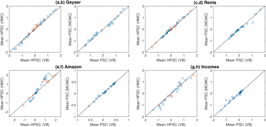
Figure K: Parameter estimates of $\beta$ (blue) and $\alpha$ (if $\neq\mathbf{0}$, red) of VB against HMC/MCMC. The datasets are (a,b) Geyser, (c,d) Rents, (e,f) Amazon, and (g,h) Incomes. HPSC is shown in panels (a,c,e,g) and PSC in panels (b,d,f,h). The close alignment shows the very high degree of accuracy of the location of the VA $q_{\lambda}$.

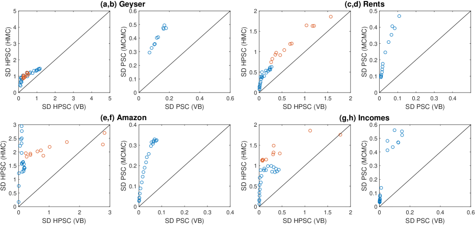
Figure L: Standard deviations of $\beta$ (blue) and $\alpha$ (if $\neq\mathbf{0}$, red) of VB against HMC/MCMC. The datasets are (a,b) Geyser, (c,d) Rents, (e,f) Amazon, and (g,h) Incomes. HPSC is shown in panels (a,c,e,g) and PSC in (b,d,f,h). Under-estimation of the posterior standard deviation of parameter values is common when using Gaussian variational approximations, although the posterior standard deviation of functionals can still be reasonably accurate; see the examples in Ong et al. (2018).

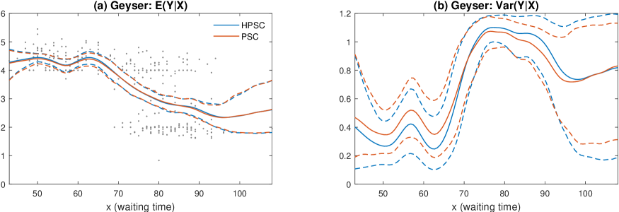
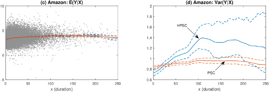
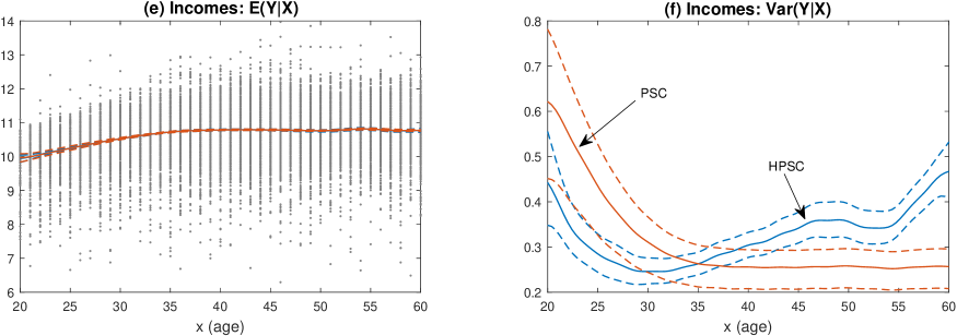
Figure M: Estimates of the regression function $f$ (left-hand side) and variance function $v$ (right-hand side) from the HPSC model, compared to those from the PSC model. The posterior means of each function are given as a solid lines, and 95% posterior intervals by dashed lines. Scatterplots of the data are included in the left-hand panels. All function estimates employ the same KDE estimator for the margins $F_{Y}$, and the datasets are (a–b) Geyser, (c–d) Amazon, (e–f) Incomes.

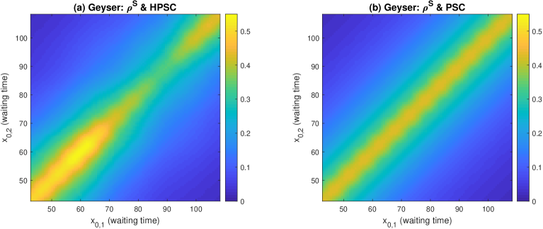
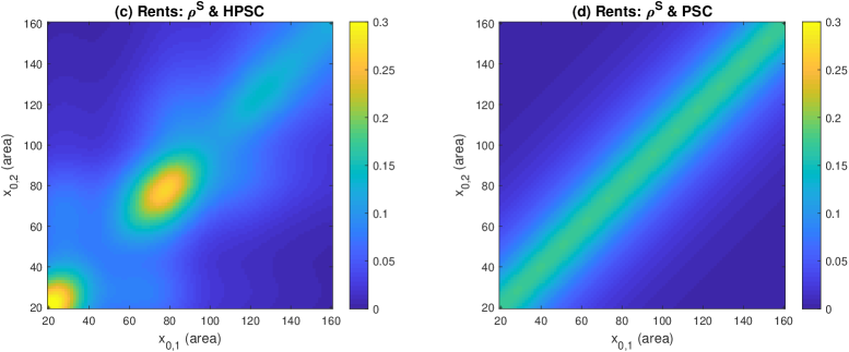
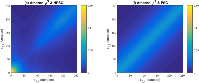
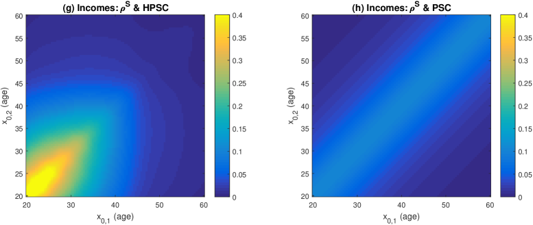
Figure N: Estimates of Spearman’s rho $\hat{\rho}^{S}(x_{0,1},x_{0,2})$. The lefthand panels give values for the HPSC, and the righthand panels for the PSC. The datasets are (a,b) Rents, (c,d) Nigeria, (e,f) Amazon, and (g,h) Incomes.

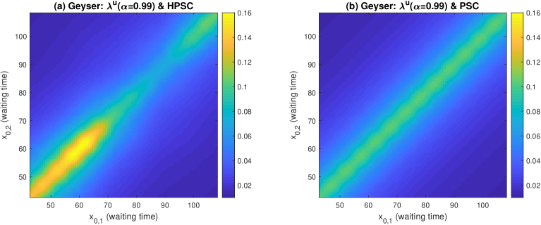
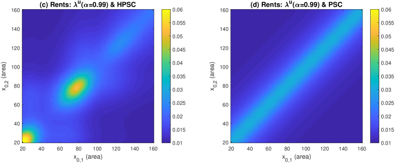
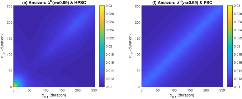
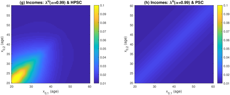
Figure O: Estimates of the upper quantile dependence $\lambda^{U}(0.99|x_{0,1},x_{0,2})$. The lefthand panels give values for the HPSC, and the righthand panels for the PSC. The datasets are (a,b) Geyser, (c,d) Rents, (e,f) Amazon, and (g,h) Incomes.

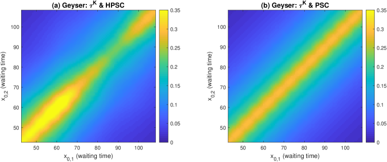
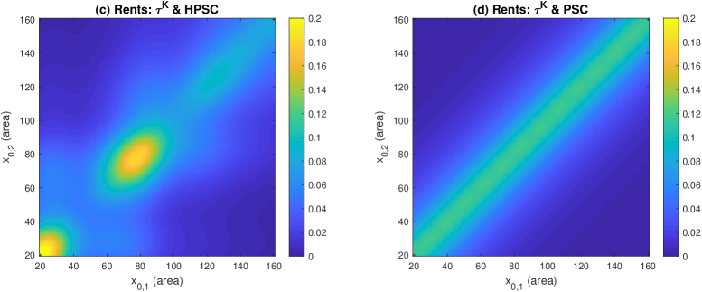
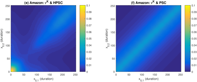
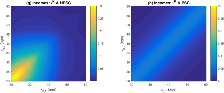
Figure P: Estimates of Kendall’s tau $\tau^{K}(x_{0,1},x_{0,2})$. The lefthand panels give values for the HPSC, and the righthand panels for the PSC. The datasets are (a,b) Geyser, (c,d) Rents, (e,f) Amazon, and (g,h) Incomes.

Appendix Part D Simulation Study Details

In this part of the appendix we provide further details for the simulation study in Section 4.2, along with additional results. The simulation designs are based on the five distributional regression methods each fitted to the four real datasets, giving a total of 20 data generating processes (DGPs) in the simulation study. Each DGP has covariate values given by those in the original dataset. For the DGPs based on the Amazon and Incomes datasets, to speed up the computations the replicates were based on sub-samples of $n=3,000$ and $n=5,000$ randomly selected covariate values from the original datasets. Similarly, we also use the faster distributional regression prediction $\hat{p}_{{\mbox{\tiny PE}}}$ defined in Section 3.4 for the regression copula models, where the point estimate used is $\text{\boldmath$\hat{\vartheta}$}_{{\mbox{\tiny VB}}}$ obtained by VB.

From each DGP we simulate 100 datasets (called ‘replicates’ here), where for each we generate $n$ observations of the response, but use the same covariate values as the original dataset. We then refit all five methods to every replicate. Accuracy of a method for each fitted replicate is assessed by using the fitted model to evaluate the predictive distributions of the observations in an additional 101${}^{\mbox{\small st}}$ replicate simulated from the DGP. Thus, we are assessing the accuracy of out-of-sample density forecasting from the same DGP. From these predictions we can construct two density forecasting measures of accuracy: the mean logarithmic score ($\overline{\mbox{LS}}$), and the mean continuous rank probability score ($\overline{\mbox{CRPS}}$) (Gneiting and Raftery, 2007), when the mean is over the density forecasts for the observations in the 101st replicate.

The results for the 5 DGPs constructed from the Incomes dataset are given in the main paper, while those for the 15 DGPs constructed from the Geyser, Rents and Amazon datasets are given in Figs. Q, R and S. The top panels of these figures give the $\overline{\mbox{LS}}$ results, and the bottom panels the corresponding $\overline{\mbox{CRPS}}$ results. Each panel corresponds to a different DGP and contains five boxplots, one for each method fit to the replicates. Each boxplot is constructed from the 100 density forecasting metrics arising from the 100 replicates. Generally speaking, one would expect refitting the same method to as used to construct the DGP, to provide the highest accuracy density forecasts. These boxplots are shaded. Therefore, our focus is on the ‘next best’ performing method. And here the HPSC method performs particularly well, being the ‘next best’ in more cases than the other approaches. In particular, HPSC either equals or out-performs the MLT benchmark method for all DGPs and metrics, except for the PS DGP.

Last, we note here how we simulate from the fitted models to construct the replicates. For the PS and HPS we extract the estimated mean (and variance) functions for the response $Y$, and simulate from the resulting normal distributions. For the MLT we extract the estimated transformation function, and use the simulate.mlt in the R package ‘mlt’. For the PSC and HPSC we extract the estimates of the mean function $\tilde{m}$ (and variance function $g$) for the pseudo-response $\tilde{Z}$, along with the estimated margin $\hat{F}_{Y}$. Simulation is then based on generating values from the conditionally Gaussian pseudo-response model, and applying the transformation $\hat{F}_{Y}^{-1}\circ\Phi$ to these values.

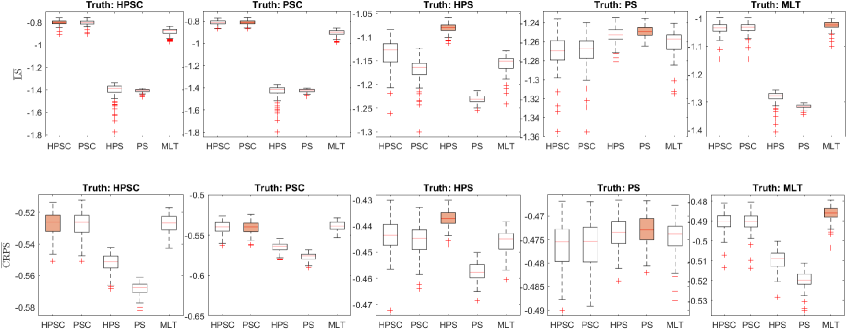
Figure Q: Simulation results for the DGPs constructed from fits to the Geyser dataset.

The top panels report the mean logarithmic score ($\overline{\mbox{LS}}$), and the bottom panels the mean CRPS ($\overline{\mbox{CRPS}}$). These are out-of-sample density forecasting metrics averaged over observations in a 101st replicate. Results are orientated so that higher values correspond to greater accuracy. The columns give results for replicates simulated from each of the DGPs obtained from fitting the five distributional regression models to the original data. In each panel boxplots of the metrics for each the 100 replicates are given, with one boxplot for each of the five methods. The shaded boxplots are for the cases where the method matches the DGP used to generate the data, which will typically be most accurate.

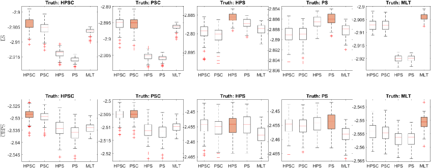
Figure R: Simulation results for the DGPs constructed from fits to the Rents dataset.

The top panels report the mean logarithmic score ($\overline{\mbox{LS}}$), and the bottom panels the mean CRPS ($\overline{\mbox{CRPS}}$). These are out-of-sample density forecasting metrics averaged over observations in a 101st replicate. Results are orientated so that higher values correspond to greater accuracy. The columns give results for replicates simulated from each of the DGPs obtained from fitting the five distributional regression models to the original data. In each panel boxplots of the metrics for each the 100 replicates are given, with one boxplot for each of the five methods. The shaded boxplots are for the cases where the method matches the DGP used to generate the data, which will typically be most accurate.

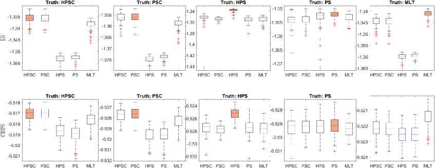
Figure S: Simulation results for the DGPs constructed from fits to the Amazon dataset.

The top panels report the mean logarithmic score ($\overline{\mbox{LS}}$), and the bottom panels the mean CRPS ($\overline{\mbox{CRPS}}$). These are out-of-sample density forecasting metrics averaged over observations in a 101st replicate. Results are orientated so that higher values correspond to greater accuracy. The columns give results for replicates simulated from each of the DGPs obtained from fitting the five distributional regression models to the original data. In each panel boxplots of the metrics for each the 100 replicates are given, with one boxplot for each of the five methods. The shaded boxplots are for the cases where the method matches the DGP used to generate the data, which will typically be most accurate.

Appendix Part E Details and Derivations for Section 5

To implement Algorithm 2 a similar strategy as described in Section Part B.2 can be used. In particular, the gradients for $\beta$ and $\alpha$ only change in the design matrices $B(\text{\boldmath$x$}),V(\text{\boldmath$w$})$ (see Section 5.1 of the main paper for the specification) and the prior precision matrices $P_{\beta},P_{\alpha}$. The latter depend on the prior choice which we discuss now.

Part E.1 Specification of the Horseshoe Prior for the Copula Parameters

For the parameters $\{\text{\boldmath$\theta$}_{\beta},\text{\boldmath$\theta$}_{\alpha}\}$ we employ the horseshoe prior such that

$$\text{\boldmath$\theta$}_{\beta}=\{\lambda_{\beta,1},\ldots,\lambda_{\beta,p_{1}},\tau_{\beta}\}\quad\text{\boldmath$\theta$}_{\alpha}=\{\lambda_{\alpha,1},\ldots,\lambda_{\alpha,p_{2}},\tau_{\alpha}\},$$

($p_{1}=240$, $p_{2}=96$ in our example), with prior distributions

$$\beta_{j}|\lambda_{j}\sim\operatorname{N}(0,\lambda_{\beta,j}^{2}),\quad\lambda_{\beta,j}|\tau_{\beta}\sim\mbox{C}^{+}(0,\tau_{\beta}),\quad\tau_{\beta}\sim\mbox{C}^{+}(0,1),\quad j=1,\ldots p_{1}$$

and similar for $\alpha$. Here, $\mbox{C}^{+}(\cdot)$ denotes a half Cauchy distribution. As a result, we obtain

$$P_{\beta}(\text{\boldmath$\theta$}_{\beta})=\operatorname{diag}(\lambda_{\beta,1}^{2},\ldots,\lambda_{\beta,p_{1}}^{2})^{-1},\quad P_{\alpha}(\text{\boldmath$\theta$}_{\alpha})=\operatorname{diag}(\lambda_{\alpha,1}^{2},\ldots,\lambda_{\alpha,p_{2}}^{2})^{-1},$$

such that $S(\text{\boldmath$x$},\text{\boldmath$w$},\text{\boldmath$\alpha$},\text{\boldmath$\lambda$}_{\beta})=\operatorname{diag}(s_{1},\ldots,s_{n})$ and

$$s_{i}=[\exp(\text{\boldmath$v$}_{i}^{\prime}\text{\boldmath$\alpha$}+\text{\boldmath$b$}_{i}^{\prime}\operatorname{diag}(\lambda_{\beta,1}^{2},\ldots,\lambda_{\beta,p_{1}}^{2})\text{\boldmath$b$}_{i})]^{-1/2}.$$

Part E.2 Log Posterior Distribution

The joint log-posterior distribution $\log(h(\text{\boldmath$\vartheta$}))=l_{\text{\boldmath$\vartheta$}}$ of

$$\text{\boldmath$\vartheta$}=\{\text{\boldmath$\beta$},\text{\boldmath$\alpha$},\log(\lambda_{\beta,1}^{2}),\ldots,\log(\lambda_{\beta,p_{1}}^{2}),\log(\tau_{\beta}),\log(\lambda_{\alpha,1}^{2}),\ldots,\log(\lambda_{\alpha,p_{2}}^{2}),\log(\tau_{\alpha})\}$$

is proportional to

$$l_{\text{\boldmath$\vartheta$}} \propto-\frac{1}{2}\sum_{i=1}^{n}(\log(s_{i}^{2}))-\frac{1}{2}\sum_{i=1}^{n}(\log(\sigma_{i}^{2}))-\frac{1}{2}(\text{\boldmath$z$}-SB\text{\boldmath$\beta$})^{\prime}(S\Sigma S)^{-1}(\text{\boldmath$z$}-SB\text{\boldmath$\beta$})$$

$$\quad+\frac{1}{2}\sum_{j=1}^{p_{1}}(\log(\lambda_{\beta,j}^{2}))-\frac{1}{2}\sum_{j=1}^{p_{1}}\frac{\beta_{j}^{2}}{\lambda_{\beta,j}^{2}}+\quad\frac{1}{2}\sum_{j=1}^{p_{2}}(\log(\lambda_{\alpha,j}^{2}))-\frac{1}{2}\sum_{j=1}^{p_{2}}\frac{\alpha_{j}^{2}}{\lambda_{\alpha,j}^{2}}$$

$$\quad-(p_{1}-1)\log(\tau_{\beta})-\sum_{j=1}^{p_{1}}\log\left(1+\frac{\lambda_{\beta,j}^{2}2}{\tau_{\beta}^{2}}\right)-(p_{2}-1)\log(\tau_{\alpha})-\sum_{j=1}^{p_{2}}\log\left(1+\frac{\lambda_{\alpha,j}^{2}2}{\tau_{\alpha}^{2}}\right)$$

$$\quad-\log(1+\tau_{\beta}^{2})-\log(1+\tau_{\alpha}^{2}),$$

and where we transform $\lambda_{\cdot,j}^{2}$ and $\tau_{\cdot}$ to the log-scale for convenience.

Part E.3 Gradients of $\log(\lambda_{\beta,j}^{2})$

$$\nabla_{\log(\lambda_{\beta,j}^{2})}l_{\text{\boldmath$\vartheta$}} =\frac{1}{2}\frac{\beta_{j}^{2}}{\lambda_{\beta,j}^{2}}-\frac{\lambda_{\beta,j}^{2}/\tau_{\beta}^{2}}{1+\lambda_{\beta,j}^{2}/\tau_{\beta}^{2}}+\frac{1}{2}+\frac{1}{2}\sum_{i=1}^{n}b_{ij}^{2}\lambda_{\beta,j}^{2}s_{i}^{2}-\frac{1}{2}\sum_{i=1}^{n}\frac{z_{i}^{2}b_{ij}^{2}\lambda_{\beta,j}^{2}}{\sigma_{i}^{2}}+\frac{1}{2}\text{\boldmath$\beta$}^{\prime}B^{\prime}(W\Sigma^{-1}S)\text{\boldmath$z$},$$

where $b_{ij}$ is the $j$-th element of $\text{\boldmath$b$}_{i}$ and $W=\operatorname{diag}(w_{1},\ldots,w_{n})$, $w_{i}=b_{ij}^{2}\lambda_{\beta,j}^{2}$.

Part E.4 Gradient of $\log(\tau_{\beta})$

$$\nabla_{\log(\tau_{\beta})}l_{\text{\boldmath$\vartheta$}} =-(p_{1}-1)+2\sum_{j=1}^{p_{1}}\frac{\lambda_{\beta,j}^{2}}{\tau_{\beta}^{2}}\left(1+\frac{\lambda_{\beta,j}^{2}}{\tau_{\beta}^{2}}\right)^{-1}-2\frac{\tau_{\beta}^{2}}{1+\tau_{\beta}^{2}}.$$

Part E.5 Gradients of $\log(\lambda_{\alpha,j}^{2})$

$$\nabla_{\log(\lambda_{\alpha,j}^{2})}l_{\text{\boldmath$\vartheta$}} =\frac{1}{2}\frac{\alpha^{2}}{\lambda_{\alpha,j}^{2}}-\frac{\lambda_{\alpha,j}^{2}/\tau_{\alpha}^{2}}{1+\lambda_{\alpha,j}^{2}/\tau_{\alpha}^{2}}+\frac{1}{2}.$$

Part E.6 Gradient of $\log(\tau_{\alpha})$

$$\nabla_{\log(\tau_{\alpha})}l_{\text{\boldmath$\vartheta$}} =-(p_{2}-1)+2\sum_{j=1}^{p_{2}}\frac{\lambda_{\alpha,j}^{2}}{\tau_{\alpha}^{2}}\left(1+\frac{\lambda_{\alpha,j}^{2}}{\tau_{\alpha}^{2}}\right)^{-1}-2\frac{\tau_{\alpha}^{2}}{1+\tau_{\alpha}^{2}}.$$

Appendix Part F Additional Figures for Section 5

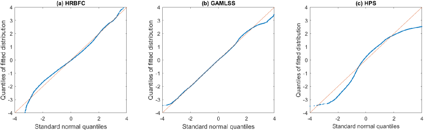
Figure T: Quantile-Quantile (QQ) plots of the residuals of three distributional regression models fit to the electricity price data

The residuals are obtained using the mean of $Y=\log(\mbox{Price}+101)$ for all $87,648$ observations, computed from the (a) HRBFC regression copula, (b) GAMLSS and (c) HPS models.

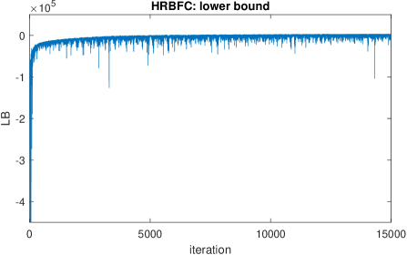
Figure U: Plot of lower bound ${\cal L}(\text{\boldmath$\lambda$})$ against step number in the SGA algorithm for the electricity price data

We note that due to the large sample size and large number of basis terms, this example is the slowest to compute. A total of 1000 steps of the SGA algorithm takes approximately 180 minutes to execute on a contemporary laptop, with code written in Matlab.

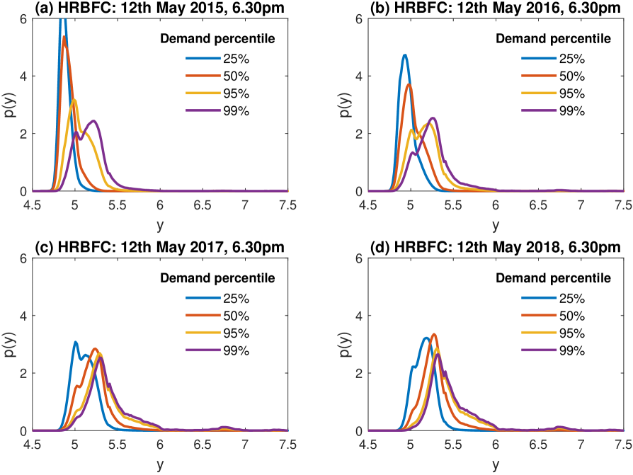
Figure V: Predictive distributions of the logarithm of electricity prices from the HRBFC regression copula model.

The four panels provide predictions for 18:30 on 12 May in the years (a) 2015 (b) 2016, (c) 2017 and (d) 2018. In each panel, the predictive densities are constructed at four levels of demand corresponding to the 0.25, 0.5, 0.95 and 0.99 percentiles of demand at 18:30. Note the accentuation of the upper tail of price from 2015 to 2018.

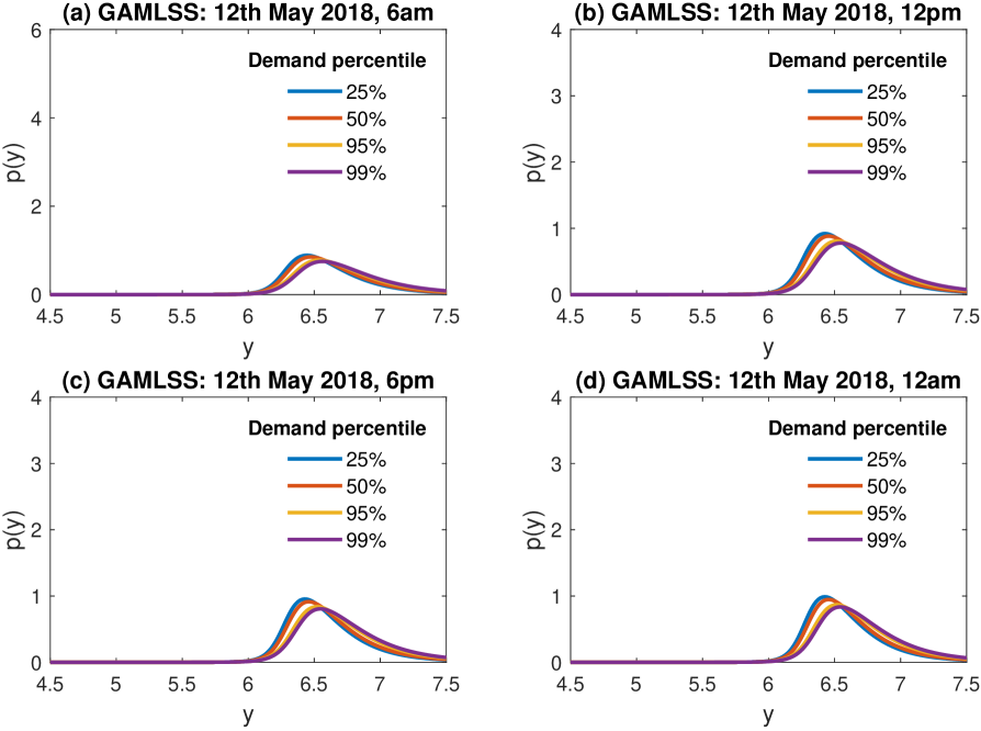
Figure W: Predictive distributions of the logarithm of electricity prices from the GAMLSS model.

The four panels provide predictions for 12 May 2018 at (a) 06:00, (b) 12:00, (c) 18:00 and (d) 24:00. In each panel, the predictive densities are constructed at four levels of demand corresponding to the 0.25, 0.5, 0.95 and 0.99 percentiles of demand at each time of day.

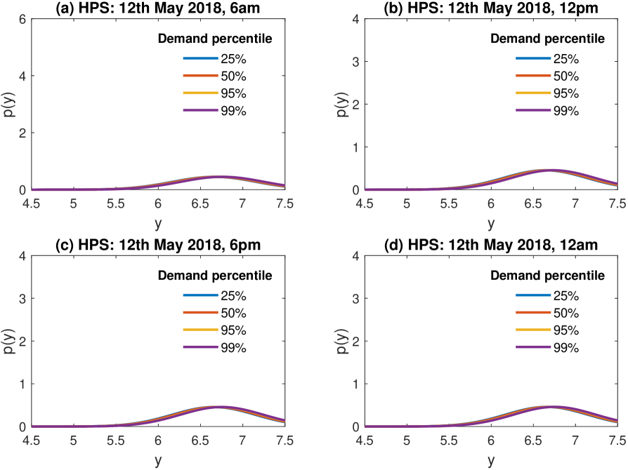
Figure X: Predictive distributions of the logarithm of electricity prices from the HPS model.

The four panels provide predictions for 12 May 2018 at (a) 06:00, (b) 12:00, (c) 18:00 and (d) 24:00. In each panel, the predictive densities are constructed at four levels of demand corresponding to the 0.25, 0.5, 0.95 and 0.99 percentiles of demand at each time of day.

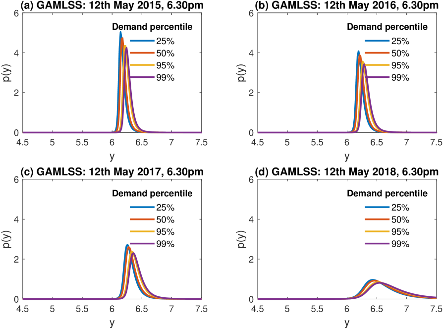
Figure Y: Predictive distributions of the logarithm of electricity prices from the GAMLSS model.

The four panels provide predictions for 18:30 on 12 May in the years (a) 2015 (b) 2016, (c) 2017 and (d) 2018. In each panel, the predictive densities are constructed at four levels of demand corresponding to the 0.25, 0.5, 0.95 and 0.99 percentiles of demand at 18:30. Note the accentuation of the upper tail of price from 2015 to 2018.

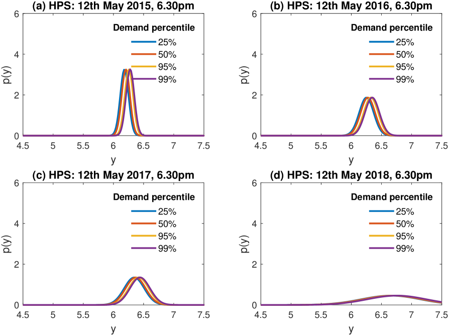
Figure Z: Predictive distributions of the logarithm of electricity prices from the HPS model.

The four panels provide predictions for 18:30 on 12 May in the years (a) 2015 (b) 2016, (c) 2017 and (d) 2018. In each panel, the predictive densities are constructed at four levels of demand corresponding to the 0.25, 0.5, 0.95 and 0.99 percentiles of demand at 18:30. Note the increase in variance from 2015 to 2018.

References

- (1)
- Aas et al. (2009) Aas, K., Czado, C., Frigessi, A. and Bakken, H. (2009). Pair-copula constructions of multiple dependence, Insurance: Mathematics and Economics 44: 182–198.
- Barndorff-Nielsen and Schou (1973) Barndorff-Nielsen, O. and Schou, G. (1973). On the parametrization of autoregressive models by partial autocorrelations, Journal of Multivariate Analysis 3(4): 408–419.
- Bottou (2010) Bottou, L. (2010). Large-scale machine learning with stochastic gradient descent, in Y. Lechevallier and G. Saporta (eds), Proceedings of the 19th International Conference on Computational Statistics (COMPSTAT2010), Springer, pp. 177–187.
- Bunn et al. (2016) Bunn, D., Andresen, A., Chen, D. and Westgaard, S. (2016). Analysis and forecasting of electricty price risks with quantile factor models, The Energy Journal 37(1).
- Chib and Jeliazkov (2006) Chib, S. and Jeliazkov, I. (2006). Inference in semiparametric dynamic models for binary longitudinal data, Journal of the American Statistical Association 101(474): 685–700.
- Demarta and McNeil (2005) Demarta, S. and McNeil, A. J. (2005). The t copula and related copulas, International Statistical Review 73(1): 111–129.
- Fahrmeir et al. (2013) Fahrmeir, L., Kneib, T., Lang, S. and Marx, B. (2013). Regression - Models, Methods and Applications, Springer, Berlin.
- Gianfreda and Bunn (2018) Gianfreda, A. and Bunn, D. (2018). A stochastic latent moment model for electricity price formation, Operations Research 66(5): 1189–1203.
- Gneiting and Raftery (2007) Gneiting, T. and Raftery, A. E. (2007). Strictly proper scoring rules, prediction, and estimation, Journal of the American Statistical Association 102: 359–378.
- Gneiting and Ranjan (2011) Gneiting, T. and Ranjan, R. (2011). Comparing density forecasts using threshold and quantile-weighted scoring rules, Journal of Business & Economic Statistics 29: 411–422.
- Grazian and Liseo (2017) Grazian, C. and Liseo, B. (2017). Approximate Bayesian inference in semiparametric copula models, Bayesian Analysis 12(4): 991–1016.
- Higgs and Worthington (2008) Higgs, H. and Worthington, A. (2008). Stochastic price modeling of high volatility, mean-reverting, spike-prone commodities: The Australian wholesale spot electricity market, Energy Economics 30(6): 3172–3185.
- Hoffman and Gelman (2014) Hoffman, M. D. and Gelman, A. (2014). The No-U-Turn sampler: Adaptively setting path lengths in Hamiltonian Monte Carlo, Journal of Machine Learning Research 15: 1351–1381.
- Honkela et al. (2010) Honkela, A., Raiko, T., Kuusela, M., Tornio, M. and Karhunen, J. (2010). Approximate riemannian conjugate gradient learning for fixed-form variational Bayes, Journal of Machine Learning Research 14: 1303–1347.
- Hothorn et al. (2017) Hothorn, T., Möst, L. and Bühlmann, P. (2017). Most likely transformations, Scandindavian Journal of Statistics 45(1): 110–134.
- Ignatieva and Trück (2016) Ignatieva, K. and Trück, S. (2016). Modeling spot price dependence in Australian electricity markets with applications to risk management, Computers & Operations Research 66: 415–433.
- Joe (2005) Joe, H. (2005). Asymptotic efficiency of the two-stage estimation method for copula-based models, Journal of Multivariate Analysis 94(2): 401–419.
- Jordan et al. (1999) Jordan, M. I., Ghahramani, Z., Jaakkola, T. S. and Saul, L. K. (1999). An introduction to variational methods for graphical models, Machine Learning 37(2): 183–233.
- Kingma and Welling (2014) Kingma, D. P. and Welling, M. (2014). Auto-encoding variational Bayes, Proceedings of the 2nd International Conference on Learning Representations (ICLR) 2014.
- Kirschen and Strbac (2004) Kirschen, D. and Strbac, G. (2004). Fundamentals of Power System Economics, first edn, Wiley, Chichester.
- Klein et al. (2015) Klein, N., Kneib, T., Lang, S. and Sohn, A. (2015). Bayesian structured additive distributional regression with an application to regional income inequality in Germany, The Annals of Applied Statistics 9: 1024–1052.
- Klein and Smith (2018) Klein, N. and Smith, M. S. (2018). Implicit copulas from Bayesian regularized regression smoothers, To appear in Bayesian Analysis .
- Lang and Brezger (2004) Lang, S. and Brezger, A. (2004). Bayesian P-splines, Journal of Computational and Graphical Statistics 13: 183–212.
- McNeil et al. (2005) McNeil, A. J., Frey, R. and Embrechts, R. (2005). Quantitative Risk Management: Concepts, Techniques and Tools, Princeton University Pres, Princton: NJ.
- Murray et al. (2013) Murray, J. S., Dunson, D. B., Carin, L. and Lucas, J. E. (2013). Bayesian Gaussian copula factor models for mixed data, Journal of the American Statistical Association 108(502): 656–665.
- Neal (2000) Neal, R. M. (2000). Markov Chain sampling methods for Dirichlet process mixture models, Journal of Computational and Graphical Statistics 9: 249–265.
- Neal (2011) Neal, R. M. (2011). MCMC using Hamiltonian dynamics, in S. Brooks, A. Gelman, G. Jones and X.-L. Meng (eds), Handbook of Markov Chain Monte Carlo, Chapman & Hall / CRC Press, pp. 113–162.
- Nelsen (2006) Nelsen, R. (2006). An Introduction to Copulas, 2nd edn, Springer.
- Oh and Patton (2017) Oh, D. H. and Patton, A. J. (2017). Modeling dependence in high dimensions with factor copulas, Journal of Business & Economic Statistics 35(1): 139–154.
- Ong et al. (2018) Ong, V. M., Nott, D. and Smith, M. (2018). Gaussian variational approximation with a factor covariance structure, Journal of Computational and Graphical Statistics 27(2): 465–478.
- Ormerod and Wand (2010) Ormerod, J. T. and Wand, M. P. (2010). Explaining variational approximations, The American Statistician 64(2): 140–153.
- Panagiotelis et al. (2014) Panagiotelis, A., Smith, M. S. and Danaher, P. J. (2014). From Amazon to Apple: Modeling online retail sales, purchase incidence, and visit behavior, Journal of Business & Economic Statistics 32: 14–29.
- Pitt et al. (2006) Pitt, M., Chan, D. and Kohn, R. (2006). Efficient Bayesian inference for Gaussian copula regression models, Biometrika 93: 537–554.
- Rezende et al. (2014) Rezende, D. J., Mohamed, S. and Wierstra, D. (2014). Stochastic backpropagation and approximate inference in deep generative models, in E. P. Xing and T. J. T. (eds), Proceedings of the 29th International Conference on Machine Learning, ICML 2014.
- Rigby and Stasinopoulos (2005) Rigby, R. A. and Stasinopoulos, D. M. (2005). Generalized additive models for location, scale and shape (with discussion), Journal of the Royal Statistical Society. Series C (Applied Statistics) 54: 507–554.
- Salimans and Knowles (2013) Salimans, T. and Knowles, D. A. (2013). Fixed-form variational posterior approximation through stochastic linear regression, Bayesian Analysis 8: 741–908.
- Shimazaki and Shinomoto (2010) Shimazaki, H. and Shinomoto, S. (2010). Kernel bandwidth optimization in spike rate estimation, Jorunal of Computational Neuroscience 29(1-2): 171–182.
- Smith et al. (2012) Smith, M. S., Gan, Q. and Kohn, R. (2012). Modeling dependence using skew t copulas: Bayesian inference and applications, Journal of Applied Econometrics 27(3): 500–522.
- Smith and Maneesoonthorn (2018) Smith, M. S. and Maneesoonthorn, W. (2018). Inversion copulas from nonlinear state space models with an application to inflation forecasting, International Journal of Forecasting 34(3): 389–407.
- Smith and Shively (2018) Smith, M. S. and Shively, T. S. (2018). Econometric modeling of regional electricity spot prices in the Australian market, Energy Economics 74: 886–903.
- Smith and Vahey (2016) Smith, M. S. and Vahey, S. (2016). Asymmetric forecast densities for U.S. macroeconomic variables from a Gaussian copula model of cross-sectional and serial dependence, Journal of Business and Economic Statistics 34(3): 416–434.
- Song (2000) Song, P. (2000). Multivariate dispersion models generated from Gaussian copula, Scandinavian Journal of Statistics 27(2): 305–320.
- Venables and Ripley (2002) Venables, W. N. and Ripley, B. D. (2002). Modern Applied Statistics with S, fourth edn, Springer, New York.
- Wauthier and Jordan (2010) Wauthier, F. L. and Jordan, M. I. (2010). Heavy-tailed process priors for selective shrinkage, Advances in Neural Information Processing Systems, pp. 2406–2414.
- Wilson and Ghahramani (2010) Wilson, A. G. and Ghahramani, Z. (2010). Copula processes, Advances in Neural Information Processing Systems, pp. 2460–2468.