How to Remove the Secrecy Constraints in Wireless Networks?

How to Break the Limits of Secrecy Constraints in Communication Networks?

Adding Common Randomness at the Transmitters Can Remove the Secrecy Constraints in Communication Networks

Adding Common Randomness Can Remove the Secrecy Constraints in Communication Networks

Abstract

In communication networks secrecy constraints usually incur an extra limit in capacity or generalized degrees-of-freedom (GDoF), in the sense that a penalty in capacity or GDoF is incurred due to the secrecy constraints. Over the past decades a significant amount of effort has been made by the researchers to understand the limits of secrecy constraints in communication networks. In this work, we focus on how to remove the secrecy constraints in communication networks, i.e., how to remove the GDoF penalty due to secrecy constraints. We begin with three basic settings: a two-user symmetric Gaussian interference channel with confidential messages, a symmetric Gaussian wiretap channel with a helper, and a two-user symmetric Gaussian multiple access wiretap channel. Interestingly, in this work we show that adding common randomness at the transmitters can totally remove the penalty in GDoF or GDoF region of the three settings considered here. The results reveal that adding common randomness at the transmitters is a powerful way to remove the secrecy constraints in communication networks in terms of GDoF performance. Common randomness can be generated offline. The role of the common randomness is to jam the information signal at the eavesdroppers, without causing too much interference at the legitimate receivers. To accomplish this role, a new method of Markov chain-based interference neutralization is proposed in the achievability schemes utilizing common randomness. From the practical point of view, we hope to use less common randomness to remove secrecy constraints in terms of GDoF performance. With this motivation, for most of the cases we characterize the minimal GDoF of common randomness to remove secrecy constraints, based on our derived converses and achievability.

I Introduction

For the secure communications with secrecy constraints, the confidential messages need to be transmitted reliably to the legitimate receiver(s), without leaking the confidential information to the eavesdroppers (cf. [1, 2]). In communication networks secrecy constraints usually impose an extra limit in capacity or generalized degrees-of-freedom (GDoF), in the sense that a penalty in capacity or GDoF is incurred due to secrecy constraints (cf. [2, 3, 4, 5, 6, 7, 8, 9, 10, 11, 12]). Since Shannon’s work of [1] in 1949, a significant amount of effort has been made by the researchers to understand the limits of secrecy constraints in communication networks (cf. [2, 13, 3, 4, 14, 5, 15, 6, 7, 8, 9, 16, 10, 11, 12, 17, 18, 19, 20, 21, 22, 23, 24] and the references therein). In this work, we focus on how to remove the secrecy constraints in communication networks, i.e., how to remove the GDoF penalty due to secrecy constraints.

In this work we consider three basic settings: a two-user symmetric Gaussian interference channel with secrecy constraints, a symmetric Gaussian wiretap channel with a helper, and a two-user symmetric Gaussian multiple access wiretap channel. Interestingly, we show that adding common randomness at the transmitters can remove the secrecy constraints in these three settings, i.e., it can totally remove the penalty in GDoF or GDoF region of the three settings. Let us take a two-user symmetric Gaussian interference channel as an example. For this interference channel without secrecy constraints, the GDoF is a “W” curve (see Fig. 1 and [25]). If secrecy constraints are imposed on this channel, then the secure GDoF is significantly reduced, compared to the original “W” curve (see Fig. 1 and [12]). It implies that a GDoF penalty is incurred due to secrecy constraints. Interestingly we show in this work that adding common randomness at the transmitters can totally remove the GDoF penalty due to secrecy constraints (see Fig. 1). The results reveal that adding common randomness at the transmitters is a constructive way to remove the secrecy constraints in terms of GDoF performance in communication networks.

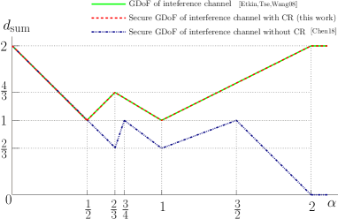
Figure 1: The optimal secure sum GDoF vs. $\alpha$, for two-user symmetric Gaussian interference channels without and with common randomness (CR), where $\alpha$ is a channel parameter indicating the interference-to-signal ratio.

The role of the common randomness is to jam the information signal at the eavesdroppers, without causing too much interference at the legitimate receivers. By jamming the information signal at the eavesdroppers with common randomness, we seek to remove the penalty in GDoF. However, the jamming signal generated from the common randomness needs to be designed carefully so that it must not create too much interference at the legitimate receivers. Otherwise, the interference will incur a new penalty in GDoF. To accomplish the role of the common randomness, a new method of Markov chain-based interference neutralization is proposed in the achievability schemes. The idea of the Markov chain-based interference neutralization method is given as follows: the common randomness is used to generate a certain number of signals with specific directions and powers; one signal is used to jam the information signal at an eavesdropper but it will create an interference at a legitimate receiver; this interference will be neutralized by another signal generated from the same common randomness; the added signal also creates another interference but will be neutralized by the next generated signal; this process repeats until the residual interference is under the noise level. Since one signal is used to neutralize the previous signal and will be neutralized by the next signal, it forms a Markov chain for this interference neutralization process.

Common randomness can be generated offline. From the practical point of view, we expect to use less common randomness to remove secrecy constraints, in terms of GDoF performance. With this motivation, we also characterize the minimal GDoF of the common randomness to remove the secrecy constraints for most of the cases, based on our derived converses and achievability.

In terms of the organization of this work, section II describes the system models and section III provides the main results. The converse is described in Section VIII. The achievability is provided in Sections V-VI and some of the appendices, while a scheme example is described in Section IV. The work is concluded in Section IX. Regarding the notations, $\mathbb{I}(\bullet)$, $\mathbb{H}(\bullet)$ and $\mathrm{h}(\bullet)$ denote the mutual information, entropy, and differential entropy, respectively. The notations of ${\mathcal{Z}}^{+}$, ${\mathcal{R}}$ and ${\mathcal{N}}$ denote the sets of positive integers, real numbers, and nonnegative integers, respectively. We define that $(\bullet)^{+}=\max\{\bullet,0\}$. We consider all the logarithms with base $2$. The notation of $f(a)=o(g(a))$ implies that $\lim_{a\to\infty}f(a)/g(a)=0$.

II The three system models

For this work we focus on three settings: a two-user interference channel with secrecy constraints, a wiretap channel with a helper, and a two-user multiple access wiretap channel. These three settings share a common channel input-output relationship, given as

$$y_{1}(t)=\sqrt{P^{\alpha_{11}}}h_{11}x_{1}(t)+\sqrt{P^{\alpha_{12}}}h_{12}x_{2}(t)+z_{1}(t),$$ (1)

$$y_{2}(t)=\sqrt{P^{\alpha_{21}}}h_{21}x_{1}(t)+\sqrt{P^{\alpha_{22}}}h_{22}x_{2}(t)+z_{2}(t),\quad t\in\{1,2,3,\cdots,n\}$$ (2)

where $x_{\ell}(t)$ represents the transmitted signal of transmitter $\ell$ at time $t$, with a normalized power constraint $\mathbb{E}|x_{\ell}(t)|^{2}\leq 1$; $y_{k}(t)$ is the signal received at receiver $k$; and $z_{k}(t)\sim\mathcal{N}(0,1)$ is the additive white Gaussian noise, for $k,\ell\in\{1,2\}$. The term $\sqrt{P^{\alpha_{k\ell}}}h_{k\ell}$ captures the channel gain between receiver $k$ and transmitter $\ell$, where $h_{k\ell}\in(1,2]$ denotes the channel coefficient. The exponent $\alpha_{k\ell}$ represents the link strength for the channel between receiver $k$ and transmitter $\ell$. The parameter $P\geq 1$ reflects the base of link strength of all the links. Note that $\sqrt{P^{\alpha_{k\ell}}}h_{k\ell}$ can represent any real channel gain bigger or equal to $1$. Thus, the above model in (1) and (2) is able to describe the general channels, in the sense of secure capacity approximation. The channel parameters $\{h_{k\ell},\alpha_{k\ell}\}_{k\ell}$ are assumed to be available at all the nodes. In this work we focus on the symmetric case such that

$$\alpha_{11}=\alpha_{22}=1,\ \alpha_{12}=\alpha_{21}=\alpha,\ \alpha>0.$$

The three settings considered here are different, mainly on the number of confidential messages, the intended receivers of the messages, and the secrecy constraints. In what follows, we will present the details of three settings.

II-A Interference channel with secrecy constraints (IC-SC)

In the setting of interference channel, transmitter $\ell$ intends to send the confidential message $w_{\ell}$ to receiver $\ell$ using $n$ channel uses, where the message $w_{\ell}$ is independently and uniformly chosen from a set $\mathcal{W}_{\ell}\operatorname*{\triangleq}\{1,2,3,\cdots,2^{nR_{\ell}}\}$, for $\ell\in\{1,2\}$. To transmit $w_{\ell}$, a function

$$f_{\ell}:\mathcal{W}_{\ell}\times\mathcal{W}_{c}\to\mathcal{R}^{n}$$

is used to map $w_{\ell}\in\mathcal{W}_{\ell}$ to the signal $x_{\ell}^{n}=f_{\ell}(w_{\ell},w_{c})\in\mathcal{R}^{n}$, where $w_{c}\in\mathcal{W}_{c}$ denotes the common randomness that is available at both transmitters but not at the receivers. We assume that $w_{c}$ is uniformly and independently chosen from a set $\mathcal{W}_{c}\operatorname*{\triangleq}\{1,2,\cdots,2^{nR_{c}}\}$. In our setting, $w_{1},w_{2}$ and $w_{c}$ are assumed to be mutually independent. The rate tuple $(R_{1}(P,\alpha),R_{2}(P,\alpha),R_{c}(P,\alpha))$ is said to be achievable if there exists a sequence of $n$-length codes such that each receiver can decode its desired message reliably, that is,

$$\text{Pr}[\hat{w_{k}}\neq w_{k}]\leq\epsilon,\quad\forall k\in\{1,2\}$$

for any $\epsilon>0$, and the transmission of the messages is secure, that is,

$$\mathbb{I}(w_{1};y_{2}^{n})\leq n\epsilon\quad\text{and}\quad\mathbb{I}(w_{2};y_{1}^{n})\leq n\epsilon$$

(known as weak secrecy constraints), as $n$ goes large. The secure capacity region $\bar{C}(P,\alpha)$ represents the collection of all the achievable rate tuples $(R_{1}(P,\alpha),R_{2}(P,\alpha),R_{c}(P,\alpha))$. The secure GDoF region $\bar{\mathcal{D}}(\alpha)$ is defined as

$$\bar{\mathcal{D}}(\alpha)\operatorname*{\triangleq} \Big{\{}(d_{1},d_{2},d_{c}):\exists\bigl{(}R_{1}(P,\alpha),R_{2}(P,\alpha),R_{c}(P,\alpha)\bigr{)}\in\bar{C}(P,\alpha)$$

$$\quad s.t.\quad d_{c}=\lim_{P\to\infty}\frac{R_{c}(P,\alpha)}{\frac{1}{2}\log P},\ d_{k}=\lim_{P\to\infty}\frac{R_{k}(P,\alpha)}{\frac{1}{2}\log P},\ \forall k\in\{1,2\}\Big{\}}.$$

The secure GDoF region $\mathcal{D}(d_{c},\alpha)$ is defined as

$$\mathcal{D}(d_{c},\alpha)\operatorname*{\triangleq}\{(d_{1},d_{2}):\exists(d_{1},d_{2},d_{c})\in\bar{\mathcal{D}}(\alpha)\}$$

which is a function of $d_{c}$ and $\alpha$. The secure sum GDoF is then defined as

$$d_{\text{sum}}(d_{c},\alpha)\operatorname*{\triangleq}\max_{d_{1},d_{2}:(d_{1},d_{2})\in\mathcal{D}(d_{c},\alpha)}d_{1}+d_{2}.$$

For this setting we are interested in the maximal (optimal) secure sum GDoF defined as

$$d^{*}_{\text{sum}}(\alpha)\operatorname*{\triangleq}\max_{d_{c}:d_{c}\geq 0}d_{\text{sum}}(d_{c},\alpha).$$

We are also interested in the minimal (optimal) GDoF of the common randomness to achieve the maximal secure sum GDoF, defined as

$$d_{c}^{*}(\alpha)\operatorname*{\triangleq}\min_{d_{c}:\ d_{\text{sum}}(d_{c},\alpha)=d^{*}_{\text{sum}}(\alpha)}d_{c}.$$

Note that degrees-of-freedom (DoF) can be treated as a specific point of GDoF by considering $\alpha_{12}=\alpha_{21}=\alpha_{22}=\alpha_{11}=1$.

II-B The wiretap channel with a helper (WTH)

In the setting of wiretap channel with a helper, transmitter 1 wishes to send the confidential message $w_{1}$ to receiver 1. This setting is slightly different from the previous interference channel setting, as transmitter 2 will just act as a helper without sending any message in this setting ($w_{2}$ can be set as empty). For transmitter 1, the mapping function $f_{1}$ is similar as that in the interference channel described in Section II-A. For transmitter 2 (helper), a function $f_{2}:\mathcal{W}_{c}\to\mathcal{R}^{n}$ maps $w_{c}\in\mathcal{W}_{c}$ to the signal $x_{2}^{n}=f_{2}(w_{c})\in\mathcal{R}^{n}$, where $w_{c}\in\mathcal{W}_{c}$ denotes the common randomness that is available at both transmitters but not at the receivers. As before, we assume that $w_{c}$ is uniformly and independently chosen from a set $\mathcal{W}_{c}=\{1,2,3,\cdots,2^{nR_{c}}\}$ and $w_{1}$ and $w_{c}$ are mutually independent. A rate pair $(R_{1}(P,\alpha),R_{c}(P,\alpha))$ is said to be achievable if there exists a sequence of $n$-length codes such that receiver 1 can reliably decode its desired message $w_{1}$ and the transmission of the message is secure such that $\mathbb{I}(w_{1};y_{2}^{n})\leq n\epsilon$, for any $\epsilon>0$ as $n$ goes large. The secure capacity region $\bar{C}(P,\alpha)$ denotes the collection of all achievable secure rate pairs $(R_{1}(P,\alpha),R_{c}(P,\alpha))$. A secure GDoF region is defined as

$$\bar{\mathcal{D}}(\alpha)\operatorname*{\triangleq}\Big{\{}(d,d_{c}):\exists\bigl{(}R_{1}(P,\alpha),R_{c}(P,\alpha)\bigr{)}\in\bar{C}(P,\alpha),\ s.t.\ d_{c}=\lim_{P\to\infty}\frac{R_{c}(P,\alpha)}{\frac{1}{2}\log P},d=\lim_{P\to\infty}\frac{R_{1}(P,\alpha)}{\frac{1}{2}\log P}\Big{\}}.$$

We are interested in the maximal (optimal) secure GDoF defined as

$$d^{*}(\alpha)\operatorname*{\triangleq}\max_{d,d_{c}:(d,d_{c})\in\bar{\mathcal{D}}(\alpha)}d.$$

We are also interested in the minimum (optimal) GDoF of the common randomness to achieve the maximal secure GDoF, defined as

$$d_{c}^{*}(\alpha)\operatorname*{\triangleq}\min_{d_{c}:(d^{*}(\alpha),d_{c})\in\bar{\mathcal{D}}(\alpha)}d_{c}.$$

II-C Multiple access wiretap channel (MAC-WT)

Let us now consider the two-user Gaussian multiple access wiretap channel. The system model of this channel is similar as that of the interference channel defined in Section II-A. One difference is that both messages $w_{1}$ and $w_{2}$ are intended to receiver 1 in this setting. Another difference is that receiver 2 now is the eavesdropper. Both messages need to be secure from receiver 2 and the secrecy constraint becomes $\mathbb{I}(w_{1},w_{2};y_{2}^{n})\leq n\epsilon$. The definitions of the rate tuple $(R_{1}(P,\alpha),R_{2}(P,\alpha),R_{c}(P,\alpha))$, secure capacity region $\bar{C}(P,\alpha)$, and secure GDoF regions $\bar{\mathcal{D}}(\alpha)$ and $\mathcal{D}(d_{c},\alpha)$ follow from that in Section II-A. In this setting, the secure GDoF region $\mathcal{D}(d_{c},\alpha)$ might not be symmetric due to the asymmetric links arriving at receiver 1. Therefore, instead of the maximal secure sum GDoF, we will focus on the maximal (optimal) secure GDoF region defined as

$$\mathcal{D}^{*}(\alpha)\operatorname*{\triangleq}\{(d_{1},d_{2}):\exists(d_{1},d_{2})\in\cup_{d_{c}}\mathcal{D}(d_{c},\alpha)\}.$$

We are also interested in the minimal (optimal) GDoF of the common randomness to achieve any given GDoF pair $(d_{1},d_{2})\in\mathcal{D}^{*}(\alpha)$, defined as

$$d_{c}^{*}(\alpha,d_{1},d_{2})\operatorname*{\triangleq}\min_{d_{c}:(d_{1},d_{2})\in\mathcal{D}(d_{c},\alpha)}d_{c}.$$

III The main results

We will provide here the main results of the channels defined in Section II. The detailed proofs are provided in Sections V-VIII, as well as the appendices.

III-A Removing the secrecy constraints

Theorem 1 (IC-SC).

For almost all the channel coefficients $\{h_{k\ell}\}\in(1,2]^{2\times 2}$ of the symmetric Gaussian IC-SC channel with common randomness (see Section II-A), the optimal characterization of the secure sum GDoF is

$$d^{*}_{\text{sum}}(\alpha)= 2(1-\alpha) 0\leq\alpha\leq\frac{1}{2}$$ for   (3a)

$$d^{*}_{\text{sum}}(\alpha)= 2\alpha \frac{1}{2}\leq\alpha\leq\frac{2}{3}$$ for   (3b)

$$d^{*}_{\text{sum}}(\alpha)= 2(1-\alpha/2) \frac{2}{3}\leq\alpha\leq 1$$ for   (3c)

$$d^{*}_{\text{sum}}(\alpha)= \alpha 1\leq\alpha\leq 2$$ for   (3d)

$$d^{*}_{\text{sum}}(\alpha)= 2 \alpha\geq 2$$ for   . (3e)

This optimal secure sum GDoF is the same as the optimal sum GDoF of the setting without any secrecy constraint.

Proof.

See Section V for the achievability proof. The optimal sum GDoF of the interference channel without secrecy constraint, which is characterized in [25], is serving as the upper bound of the secure sum GDoF of this IC-SC channel with common randomness. ∎

Note that, without secrecy constraints, the optimal sum GDoF of the interference channel is a “W” curve (see [25] and Fig. 1). With secrecy constraints, the secure sum GDoF of the interference channel is then reduced to a modified “W” curve (cf. [12]). It implies that there is a penalty in GDoF incurred by the secrecy constraints. Interestingly, Theorem 1 reveals that we can remove this penalty by adding common randomness, in terms of sum GDoF.

Theorem 2 (WTH).

Given the symmetric Gaussian WTH channel with common randomness (see Section II-B), the optimal secure GDoF is expressed by

$$d^{*}(\alpha)=1,\quad\forall\alpha\in[0,\infty),$$

which is the same as the maximal GDoF of the setting without secrecy constraint.

Proof.

See Section VI for the achievability proof. Without secrecy constraint, the WTH channel can be enhanced to a point-to-point channel, and the maximal GDoF of the point-to-point channel is $1$. ∎

For the symmetric Gaussian WTH channel without common randomness, the secure GDoF is another modified “W” curve (cf. [19]). Without secrecy constraint, the maximal GDoF of the setting is $1$. Thus, there is a penalty in GDoF due to secrecy constraint. Theorem 2 reveals that we can remove this GDoF penalty by adding common randomness.

Theorem 3 (MAC-WT).

Given the symmetric Gaussian MAC-WT channel with common randomness (see Section II-C), the optimal secure GDoF region $\mathcal{D}^{*}(\alpha)$ is the set of all pairs $(d_{1},d_{2})$ satisfying

$$d_{1}+d_{2} \leq\max\{1,\alpha\}$$ (4)

$$0\leq d_{1} \leq 1$$ (5)

$$0\leq d_{2} \leq\alpha,$$ (6)

which is the same as the optimal GDoF region of the symmetric Gaussian multiple access channel without eavesdropper, i.e., without secrecy constraint.

Proof.

The achievability proof is provided in Section VII. The optimal GDoF region of the multiple access channel without secrecy constraint is serving as the outer bound of the optimal secure GDoF region of the MAC-WT channel with common randomness. The optimal GDoF region of the symmetric Gaussian multiple access channel is characterized as in (4)-(6), which can be easily derived from the capacity region of the setting (cf. [26]). ∎

For the multiple access channel, there is a penalty in GDoF region due to secrecy constraint. For example, considering the case with $\alpha=1$, the optimal sum GDoF of the multiple access channel without secrecy constraint is $1$. With secrecy constraint, i.e., with an eavesdropper, the optimal secure sum GDoF of multiple access wiretap channel is reduced to $2/3$ (cf. [7]). Therefore, secrecy constraint incurs an extra limit on the GDoF region. Theorem 3 reveals that by adding common randomness we can achieve a secure GDoF region that is the same as the one without secrecy constraint. In other words, with common randomness, secrecy constraint will not incur any penalty in GDoF region of the symmetric multiple access wiretap channel.

III-B How much common randomness is required?

The results in Theorems 1-3 reveal that we can remove the secrecy constraints, i.e., remove the penalty in GDoF, by adding common randomness for each channel considered here. From the practical point of view, we hope to use less common randomness to remove the secrecy constraints. Therefore, it would be interesting to characterize the minimal GDoF of the common randomness to achieve this goal. The results on this perspective are given in the following theorems.

Theorem 4 (IC-SC).

For the two-user symmetric Gaussian IC-SC channel, the minimal GDoF of the common randomness to achieve the maximal secure sum GDoF $d^{*}_{\text{sum}}(\alpha)$ is

$$d_{c}^{*}(\alpha)=d^{*}_{\text{sum}}(\alpha)/2-(1-\alpha)^{+}\quad\quad\alpha\in[0,\infty).$$ (7)

Proof.

See Section V for the achievability proof and Section VIII-A for the converse proof. ∎

Theorem 5 (WTH).

For the symmetric Gaussian WTH channel, the minimal GDoF of the common randomness to achieve the maximal secure GDoF $d^{*}(\alpha)$ is

$$d_{c}^{*}(\alpha)=1-(1-\alpha)^{+}\quad\quad\alpha\in[0,\infty).$$ (8)

Proof.

See Section VI and Section VIII-B for the achievability and converse proofs, respectively. ∎

For the MAC-WT channel, we were able to characterize the minimal GDoF of the common randomness to achieve any given GDoF pair $(d_{1},d_{2})$ in the maximal secure GDoF region $\mathcal{D}^{*}(1)$ expressed in Theorem 3, for the case of $\alpha=1$.

Theorem 6 (MAC-WT).

Given the symmetric Gaussian MAC-WT channel, and for $\alpha=1$, the minimal GDoF of the common randomness to achieve any given GDoF pair $(d_{1},d_{2})$ in the maximal secure GDoF region $\mathcal{D}^{*}(1)$ is

$$d_{c}^{*}(1,d_{1},d_{2})=\max\{d_{1},d_{2}\}\quad\text{for}\quad(d_{1},d_{2})\in\mathcal{D}^{*}(1),\ \alpha=1.$$

Proof.

The achievability and converse proofs are provided in Section VII and Section VIII-C, respectively. ∎

When $\alpha=1$, Theorem 6 reveals that the minimal GDoF of the common randomness to achieve the secure GDoF pair $(d_{1}=1/2,d_{2}=1/2)\in\mathcal{D}^{*}(1)$ is 1/2. It implies that 1/2 GDoF of common randomness achieves the maximal secure sum GDoF 1. Without common randomness, the secure sum GDoF cannot be more than $2/3$ for the case with $\alpha=1$. Note that it is challenging to characterize $d_{c}^{*}(\alpha,d_{1},d_{2})$ for the general case of $\alpha$. For the general case, the optimal secure GDoF region is non-symmetric in $(d_{1},d_{2})$ as shown in Theorem 3. To achieve the GDoF pairs in the asymmetric secure GDoF region, it might require several converse bounds on the minimal GDoF of the common randomness, which will be studied in our future work.

IV Scheme example

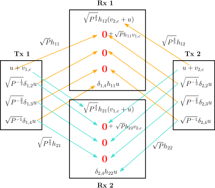
Figure 2: Markov chain-based interference neutralization at the receivers, for a two-user interference channel with $\alpha=4/3$.

We will here provide a scheme example, focusing on the IC-SC channel with $\alpha=4/3$ (see Section II-A). Note that for the case of $\alpha=4/3$, without the consideration of secrecy constraints the sum GDoF is $4/3$ (cf. [25]). With the consideration of secrecy constraints, the secure sum GDoF is reduced to $8/9$ (cf. [12]). In this example, we will show that by adding common randomness the secure sum GDoF can be improved to $4/3$, which matches the sum GDoF for the case without secrecy constraints. In our scheme, Markov chain-based interference neutralization will be used in the signal design. In this scheme, the transmitted signals are given as (without time index):

$$x_{k}=v_{k,c}+\sum_{\ell=1}^{4}\delta_{k,\ell}\sqrt{P^{-\beta_{u_{\ell}}}}\cdot u$$

for $k\in\{1,2\}$, where $\beta_{u_{\ell}}=\frac{1}{3}(\ell-1)$, for $\ell\in\{1,2,3,4\}$; and

$$\delta_{j,\ell}=\left\{\begin{array}[]{ll}-\frac{h_{ii}}{h_{ij}}\cdot\big{(}\frac{h_{11}h_{22}}{h_{12}h_{21}}\big{)}^{\frac{\ell}{2}-1}&\quad\textrm{$\ell\in\{2,4\}$}\\ \big{(}\frac{h_{11}h_{22}}{h_{12}h_{21}}\big{)}^{\frac{\ell-1}{2}}&\quad\textrm{$\ell\in\{1,3\}$}\end{array}\right.$$ (11)

for $i,j\in\{1,2\},i\not=j.$ $u$ is the common randomness. $v_{1,c}$ and $v_{2,c}$ carry the messages of transmitters 1 and 2, respectively. The random variables $v_{1,c}$, $v_{2,c}$ and $u$ are independently and uniformly drawn from a pulse amplitude modulation (PAM) set

$$v_{1,c},v_{2,c},u\in\Omega(\xi=\frac{\gamma}{Q},\quad Q=P^{\frac{2/3-\epsilon}{2}})$$

where $\gamma\in\bigl{(}0,1/64\bigr{]}$ is a constant, $\Omega(\xi,Q)\operatorname*{\triangleq}\{\xi a:\ a\in[-Q,Q]\cap{\mathcal{Z}}\}$, and $\epsilon>0$ is a parameter that can be made arbitrarily small. With this signal design, $v_{k,c}$ carries $2/3$ GDoF, i.e., $\mathbb{H}(v_{k,c})=\frac{2/3-\epsilon}{2}\log P+o(\log P)$, with $k\in\{1,2\}$. One can check that the average power constraints $\mathbb{E}|x_{1}|^{2}\leq 1$ and $\mathbb{E}|x_{2}|^{2}\leq 1$ are satisfied. Then, the received signals are given as (without time index)

$$y_{k} \!=\!\sqrt{P}h_{kk}v_{k,c}\!+\!\underbrace{\sqrt{P^{4/3}}h_{kj}v_{j,c}\!+\!\sqrt{P^{4/3}}\delta_{j,1}h_{kj}u}_{\rm{aligned}}\!+\!\sum_{\ell=1}^{3}\!\underbrace{(\sqrt{P^{(4\!-\!\ell)/3}}\delta_{k,\ell}h_{kk}\!+\!\sqrt{P^{(4\!-\!\ell)/3}}\delta_{j,\ell\!+\!1}h_{kj})u}_{\rm{interference~{}neutralization}}\!+\!\delta_{k,4}h_{kk}u\!+\!z_{k}$$

$$=\sqrt{P}h_{kk}v_{k,c}+\sqrt{P^{4/3}}h_{kj}(v_{j,c}+u)\!+\!\delta_{k,4}h_{kk}u\!+\!z_{k}$$

for $k\neq j$, $k,j\in\{1,2\}$. The idea of the Markov chain-based interference neutralization method is given as follows. As shown in Fig. 2, the common randomness $u$ is used to generate a certain number of signals with specific directions and powers, i.e., $\{\delta_{1,\ell}\sqrt{P^{-\beta_{u_{\ell}}}}u\}_{\ell=1}^{4}$ at transmitter 1 and $\{\delta_{2,\ell}\sqrt{P^{-\beta_{u_{\ell}}}}u\}_{\ell=1}^{4}$ at transmitter 2; the signal $\delta_{2,1}\sqrt{P^{-\beta_{u_{1}}}}u$ from transmitter 2 is used to jam the information signal $v_{2,c}$ at receiver 1 but it will create an interference at receiver 2; this interference will be neutralized by the signal $\delta_{1,2}\sqrt{P^{-\beta_{u_{2}}}}u$ from transmitter 1; the added signal $\delta_{1,2}\sqrt{P^{-\beta_{u_{2}}}}u$ also creates another interference at receiver 1 but will be neutralized by the next generated signal $\delta_{2,3}\sqrt{P^{-\beta_{u_{3}}}}u$; this process repeats until the residual interference is under the noise level. Since one signal is used to neutralize the previous signal and will be neutralized by the next signal, it forms a Markov chain for this interference neutralization process.

From our signal design, it can be proved that the secure rates $R_{k}=\mathbb{I}(v_{k,c};y_{k})-\mathbb{I}(v_{k,c};y_{j}|v_{j,c})\geq\frac{2/3-\epsilon}{2}\log P+o(\log P)$, $k\neq j$, $k,j\in\{1,2\}$, and the secure sum GDoF $d_{\text{sum}}=4/3$, are achievable for almost all the channel coefficients $\{h_{k\ell}\}\in(1,2]^{2\times 2}$, by using $d_{c}=2/3$ GDoF of common randomness. More details on the proposed scheme can be found in Section V.

V Achievability for interference channel

We will here provide the achievability scheme for the symmetric Gaussian IC-SC channel (see Section II-A). Our scheme uses PAM modulation, Markov chain-based interference neutralization and alignment technique in the signal design. For the case with $0\leq\alpha\leq 1/2$, the optimal secure sum GDoF is achievable without adding common randomness (cf. [25, 12]). Thus, here we will just focus on the case with $\alpha>1/2$. The scheme details are given in the following subsections.

V-1 Codebook generation

Transmitter $k$, $k=1,2$, at first generates a codebook as

$$\mathcal{B}_{k}\operatorname*{\triangleq}\Bigl{\{}v^{n}_{k}(w_{k},w^{\prime}_{k}):\ w_{k}\in\{1,2,\cdots,2^{nR_{k}}\},w^{\prime}_{k}\in\{1,2,\cdots,2^{nR^{\prime}_{k}}\}\Bigr{\}}$$ (12)

where $v^{n}_{k}$ denotes the corresponding codewords. The elements of the codewords are generated independently and identically based on a particular distribution. $w^{\prime}_{k}$ is an independent randomness that is used to protect the confidential message, and is uniformly distributed over $\{1,2,\cdots,2^{nR^{\prime}_{k}}\}$. $R_{k}$ and $R^{\prime}_{k}$ are the rates of $w_{k}$ and $w^{\prime}_{k}$, respectively. To transmit the confidential message $w_{k}$, transmitter $k$ randomly chooses a codeword $v^{n}_{k}$ from a sub-codebook $\mathcal{B}_{k}(w_{k})$ defined by

$$\mathcal{B}_{k}(w_{k})\operatorname*{\triangleq}\bigl{\{}v^{n}_{k}(w_{k},w^{\prime}_{k}):\ w^{\prime}_{k}\in\{1,2,\cdots,2^{nR^{\prime}_{k}}\}\bigr{\}},\quad k=1,2$$ (13)

according to a uniform distribution. Then, the selected codeword $v^{n}_{k}$ is mapped to the channel input based on the following signal design

$$x_{k}(t)=\varepsilon v_{k}(t)+\varepsilon\sum_{\ell=1}^{\tau}\delta_{k,\ell}\sqrt{P^{-\beta_{u_{\ell}}}}\cdot u(t)$$ (14)

for $k=1,2$, where $v_{k}(t)$ denotes the $t$th element of $v^{n}_{k}$; $\{\delta_{j,\ell}\}_{j,\ell}$ are parameters that will be designed specifically later on for different cases of $\alpha$, based on the Markov chain-based interference neutralization and alignment technique. $\varepsilon$ is a parameter designed as

$$\varepsilon\operatorname*{\triangleq}\begin{cases}1&\quad\rm{if~{}\alpha\neq 1}\\ \frac{h_{11}h_{22}-h_{12}h_{21}}{8}&\quad\rm{if~{}\alpha=1}\end{cases}$$ (15)

which is used to regularize the power of the transmitted signal. $\tau$ is a parameter designed as

$$\tau\operatorname*{\triangleq}\begin{cases}\lceil\frac{\alpha}{1-\alpha}\rceil&\quad\rm{if~{}\alpha<1}\\ \lceil\frac{\alpha}{\alpha-1}\rceil&\quad\rm{if~{}\alpha>1}\\ 1&\quad\rm{if~{}\alpha=1}.\end{cases}$$ (16)

$u$ is a random variable independently and uniformly drawn from a PAM constellation set, which will be specified later on. For the proposed scheme, the common randomness $w_{c}$ is mapped into three random variables, i.e., $w^{\prime}_{1},w^{\prime}_{2}$ and $u$, such that $\mathbb{H}(w_{c})=\mathbb{H}(w^{\prime}_{1})+\mathbb{H}(w^{\prime}_{2})+\mathbb{H}(u)$ and $w^{\prime}_{1},w^{\prime}_{2}$ and $u$ are mutually independent. Based on our definition, $w^{\prime}_{1},w^{\prime}_{2}$ and $u$ are available at the transmitters but not at the receivers.

V-2 Signal design

For transmitter $k$, $k=1,2$, each element of the codeword is designed to have the following form

$$v_{k}=v_{k,c}+\sqrt{P^{-\beta_{k,p}}}v_{k,p}.$$ (17)

With this, the input signal in (14) can be expressed as

$$x_{k}=\varepsilon v_{k,c}+\varepsilon\sqrt{P^{-\beta_{k,p}}}\cdot v_{k,p}+\varepsilon\sum_{\ell=1}^{\tau}\delta_{k,\ell}\sqrt{P^{-\beta_{u_{\ell}}}}\cdot u,\quad k=1,2$$ (18)

(without time index for simplicity), where random variables $\{v_{k,c},v_{k,p},u\}$ are independently and uniformly drawn from the following PAM constellation sets

$$v_{k,c},u \in\Omega(\xi=\frac{\gamma}{Q},\ Q=P^{\frac{\lambda_{k,c}}{2}})$$ (19)

$$v_{k,p} \in\Omega(\xi=\frac{\gamma}{2Q},\ Q=P^{\frac{\lambda_{k,p}}{2}})$$ (20)

where $\gamma$ is a parameter satisfying the constraint

$$\gamma\in\bigl{(}0,\ \frac{1}{\tau\cdot 2^{\tau}}].$$

In the proposed scheme, the designed parameters $\{\beta_{k,p},\beta_{u_{\ell}},\lambda_{k,c},\lambda_{k,p},\lambda_{u}\}_{k,\ell}$ are given in Table I for different regimes. Based on the signal design in (19) and (20), we have

$$\mathbb{E}|v_{k,c}|^{2} =\frac{2\times(\frac{\gamma}{Q})^{2}}{2Q+1}\sum_{i=1}^{Q}i^{2}=\frac{(\frac{\gamma}{Q})^{2}\cdot Q(Q+1)}{3}\leq\frac{2\gamma^{2}}{3}$$ (21)

$$\mathbb{E}|u|^{2} \leq\frac{2\gamma^{2}}{3}$$ (22)

$$\mathbb{E}|v_{k,p}|^{2} \leq\frac{\gamma^{2}}{6}.$$ (23)

From (15), (18) and (21)-(23), we can verify that the signal $x_{k}$ satisfies the power constraint, that is

$$\mathbb{E}|x_{k}|^{2}= \varepsilon^{2}\mathbb{E}|v_{k,c}|^{2}+\varepsilon^{2}P^{-\beta_{k,p}}\mathbb{E}|v_{k,p}|^{2}+\varepsilon^{2}\big{(}\sum_{\ell=1}^{\tau}\delta_{k,\ell}P^{-\beta_{u_{\ell}}}\big{)}^{2}\mathbb{E}|u|^{2}$$

$$\leq \varepsilon^{2}\times\frac{2\gamma^{2}}{3}+\varepsilon^{2}\times\frac{\gamma^{2}}{6}+\varepsilon^{2}\times\tau^{2}4^{\tau}\times\frac{2\gamma^{2}}{3}$$

$$\leq 1$$

for $k=1,2$, where $\gamma\in\bigl{(}0,\frac{1}{\tau\cdot 2^{\tau}}\bigr{]}$, $\varepsilon^{2}\leq 1$ and $\delta_{k,\ell}$ is designed specifically for different cases of $\alpha$ satisfying the inequality $\varepsilon^{2}\delta^{2}_{k,\ell}\leq 4^{\tau},\forall k,\ell$, which will be shown later on.

V-3 Secure rate analysis

We define the rates $R_{k}$ and $R_{k}^{\prime}$ as

$$R_{k} \operatorname*{\triangleq}\mathbb{I}(v_{k};y_{k})-\mathbb{I}(v_{k};y_{\ell}|v_{\ell})-\epsilon$$ (24)

$$R_{k}^{\prime} \operatorname*{\triangleq}\mathbb{I}(v_{k};y_{\ell}|v_{\ell})-\epsilon$$ (25)

for some $\epsilon>0$, and $\ell,k\in\{1,2\},\ell\neq k$. With our codebook and signal design, the result of [8, Theorem 2] (or [3, Theorem 2]) suggests that the rate pair $(R_{1},R_{2})$ defined above is achievable and the transmission of the messages is secure, i.e., $\mathbb{I}(w_{1};y_{2}^{n})\leq n\epsilon$ and $\mathbb{I}(w_{2};y_{1}^{n})\leq n\epsilon$. Remind that, based on our codebook design, $v_{1}$ and $v_{2}$ are independent, since $w_{1},w_{2},w^{\prime}_{1},w^{\prime}_{2}$ are mutually independent (cf. (12)).

In what follows we will show how to remove the secrecy constraints in terms of GDoF performance by adding common randomness, focusing on the regime of $\alpha>1/2$. Specifically, we will consider the following five cases: $\frac{2}{3}\leq\alpha<1$, $1<\alpha\leq 2$, $\alpha=1$, $\frac{1}{2}<\alpha\leq\frac{2}{3}$, and $2\leq\alpha$. In the achievability scheme, a Markov chain-based interference neutralization method is proposed to accomplish the role of common randomness.

TABLE I: Parameter design for the IC-SC channel.

	$\frac{1}{2}<\alpha\leq\frac{2}{3}$	$\frac{2}{3}\leq\alpha<1$	$\alpha=1$	$1<\alpha\leq 2$	$2\leq\alpha$
$\beta_{u_{\ell}},\ell\in\{\!1,\!2,\cdots\!,\!\tau\!\}$	$(1\!-\!\alpha)\ell$	$(1\!-\!\alpha)\ell$	$0$	$(\alpha\!-\!1)(\ell\!-\!1)$	$(\alpha\!-\!1)(\ell\!-\!1)$
$\beta_{1,p},\ \beta_{2,p}$	$\alpha$	$\alpha$	$\infty$	$\infty$	$\infty$
$\lambda_{1,c},\ \lambda_{2,c}$	$2\alpha-1-\epsilon$	$\alpha/2-\epsilon$	$1/2-\epsilon$	$\alpha/2-\epsilon$	$1-\epsilon$
$\lambda_{u}$	$2\alpha-1-\epsilon$	$\alpha/2-\epsilon$	$1/2-\epsilon$	$\alpha/2-\epsilon$	$1-\epsilon$
$\lambda_{1,p},\ \lambda_{2,p}$	$1-\alpha-\epsilon$	$1-\alpha-\epsilon$	$0$	$0$	0

V-A $2/3\leq\alpha<1$

In this case with $2/3\leq\alpha<1$, based on the parameters designed in Table I, the transmitted signals take the following forms

$$x_{1}= v_{1,c}+\sqrt{P^{-\alpha}}\cdot v_{1,p}+\sum_{\ell=1}^{\tau}\delta_{1,\ell}\sqrt{P^{-\beta_{u_{\ell}}}}\cdot u$$ (26)

$$x_{2}= v_{2,c}+\sqrt{P^{-\alpha}}\cdot v_{2,p}+\sum_{\ell=1}^{\tau}\delta_{2,\ell}\sqrt{P^{-\beta_{u_{\ell}}}}\cdot u$$ (27)

where the parameters $\{\delta_{j,\ell}\}_{j,\ell}$ are designed as

$$\delta_{j,\ell}=\left\{\begin{array}[]{ll}-\big{(}\frac{h_{12}h_{21}}{h_{11}h_{22}}\big{)}^{\frac{\ell}{2}}&\quad\textrm{$\ell\in\{2k:2k\leq\tau,k\in{\mathcal{Z}}^{+}\}$}\\ &\\ \frac{h_{ji}}{h_{jj}}\cdot\big{(}\frac{h_{12}h_{21}}{h_{11}h_{22}}\big{)}^{\frac{\ell-1}{2}}&\quad\textrm{$\ell\in\{2k-1:2k-1\leq\tau,k\in{\mathcal{Z}}^{+}\}$}\end{array}\right.$$ (31)

for $i,j\in\{1,2\},i\not=j.$ Note that the common randomness $u$ is used to generate a certain number of signals with specific directions and powers, i.e., $\{\delta_{1,\ell}\sqrt{P^{-\beta_{u_{\ell}}}}u\}_{\ell=1}^{\tau}$ at transmitter 1 and $\{\delta_{2,\ell}\sqrt{P^{-\beta_{u_{\ell}}}}u\}_{\ell=1}^{\tau}$ at transmitter 2. Then, the received signals are expressed as

$$y_{1} =\sqrt{P}h_{11}v_{1,c}+\sqrt{P^{1-\alpha}}h_{11}v_{1,p}+\underbrace{\sqrt{P^{\alpha}}h_{12}v_{2,c}+\sqrt{P^{1-\beta_{u_{1}}}}\delta_{1,1}h_{11}u}_{\rm{aligned}}$$

$$\quad+\sum_{\ell=1}^{\tau-1}\underbrace{(\sqrt{P^{1-\beta_{u_{\ell+1}}}}\delta_{1,\ell+1}h_{11}+\sqrt{P^{\alpha-\beta_{u_{\ell}}}}\delta_{2,\ell}h_{12})u}_{\rm{interference~{}neutralization}}+\underbrace{\sqrt{P^{(\tau+1)\alpha-\tau}}\delta_{2,\tau}h_{12}u+h_{12}v_{2,p}}_{\text{treated as noise}}+z_{1}$$

$$=\sqrt{P}h_{11}v_{1,c}+\sqrt{P^{1-\alpha}}h_{11}v_{1,p}+\sqrt{P^{\alpha}}h_{12}(v_{2,c}+u)+\sqrt{P^{(\tau+1)\alpha-\tau}}\delta_{2,\tau}h_{12}u+h_{12}v_{2,p}+z_{1}$$ (32)

$$y_{2} =\sqrt{P}h_{22}v_{2,c}+\sqrt{P^{1-\alpha}}h_{22}v_{2,p}+\underbrace{\sqrt{P^{\alpha}}h_{21}v_{1,c}+\sqrt{P^{1-\beta_{u_{1}}}}\delta_{2,1}h_{22}u}_{\rm{aligned}}$$

$$\quad+\sum_{\ell=1}^{\tau-1}\underbrace{(\sqrt{P^{1-\beta_{u_{\ell+1}}}}\delta_{2,\ell+1}h_{22}+\sqrt{P^{\alpha-\beta_{u_{\ell}}}}\delta_{1,\ell}h_{21})u}_{\rm{interference~{}neutralization}}+\underbrace{\sqrt{P^{(\tau+1)\alpha-\tau}}\delta_{1,\tau}h_{21}u+h_{21}v_{1,p}}_{\text{treated as noise}}+z_{2}$$

$$=\sqrt{P}h_{22}v_{2,c}+\sqrt{P^{1-\alpha}}h_{22}v_{2,p}+\sqrt{P^{\alpha}}h_{21}(v_{1,c}+u)+\sqrt{P^{(\tau+1)\alpha-\tau}}\delta_{1,\tau}h_{21}u+h_{21}v_{1,p}+z_{2}.$$ (33)

At the receivers, a Markov chain-based interference neutralization method is used to remove the interference. In the above expressions of $y_{1}$ and $y_{2}$, we can see that the signal $\delta_{1,1}\sqrt{P^{-\beta_{u_{1}}}}u$ from transmitter  1 is used to jam the information signal $v_{2,c}$ at receiver 1 but it will create an interference at receiver 2; this interference will be neutralized by the signal $\delta_{2,2}\sqrt{P^{-\beta_{u_{2}}}}u$ from transmitter 2; the added signal $\delta_{2,2}\sqrt{P^{-\beta_{u_{2}}}}u$ also creates another interference at receiver 1 but will be neutralized by the next generated signal $\delta_{1,3}\sqrt{P^{-\beta_{u_{3}}}}u$; this process repeats until the residual interference can be treated as noise, that is, both interference $\sqrt{P^{(\tau+1)\alpha-\tau}}\delta_{2,\tau}h_{12}u$ and $\sqrt{P^{(\tau+1)\alpha-\tau}}\delta_{1,\tau}h_{21}u$ can be treated as noise terms at receiver 1 and receiver 2, respectively.

Based on our signal design, we will prove that the secure rates satisfy $R_{k}=\mathbb{I}(v_{k};y_{k})-\mathbb{I}(v_{k};y_{\ell}|v_{\ell})\geq\frac{1-\alpha/2-2\epsilon}{2}\log P+o(\log P)$, for $k,\ell\in\{1,2\}$, $k\neq\ell$, and the secure sum GDoF $d_{\text{sum}}=2(1-\alpha/2)$ is achievable, for almost all the realizations of the channel coefficients $\{h_{k\ell}\}\in(1,2]^{2\times 2}$. For the secure rates described in (24), letting $\epsilon\to 0$ gives

$$R_{1} =\mathbb{I}(v_{1};y_{1})-\mathbb{I}(v_{1};y_{2}|v_{2})$$ (34)

$$R_{2} =\mathbb{I}(v_{2};y_{2})-\mathbb{I}(v_{2};y_{1}|v_{1}).$$ (35)

Due to the symmetry we will focus on bounding the secure rate $R_{1}$ (see (34)). We will use $\hat{v}_{1,c}$ and $\hat{v}_{1,p}$ to denote the estimates for $v_{1,c}$ and $v_{1,p}$ respectively from $y_{1}$, and use $\text{Pr}[\{v_{1,c}\neq\hat{v}_{1,c}\}\cup\{v_{1,p}\neq\hat{v}_{1,p}\}]$ to represent the error probability of this estimation. Then the term $\mathbb{I}(v_{1};y_{1})$ can be lower bounded by

$$\mathbb{I}(v_{1};y_{1})$$

$$\geq \mathbb{I}(v_{1};\hat{v}_{1,c},\hat{v}_{1,p})$$ (36)

$$= \mathbb{H}(v_{1})-\mathbb{H}(v_{1}|\hat{v}_{1,c},\hat{v}_{1,p})$$

$$\geq \mathbb{H}(v_{1})-\bigl{(}1+\text{Pr}[\{v_{1,c}\neq\hat{v}_{1,c}\}\cup\{v_{1,p}\neq\hat{v}_{1,p}\}]\cdot\mathbb{H}(v_{1})\bigr{)}$$ (37)

$$= \bigl{(}1-\text{Pr}[\{v_{1,c}\neq\hat{v}_{1,c}\}\cup\{v_{1,p}\neq\hat{v}_{1,p}\}]\bigr{)}\cdot\mathbb{H}(v_{1})-1$$ (38)

where (36) results from the Markov chain $v_{1}\to y_{1}\to\{\hat{v}_{1,c},\hat{v}_{1,p}\}$; (37) uses Fano’s inequality. The rates of $v_{1,c}$, $v_{1,p}$ and $v_{1}=v_{1,c}+\sqrt{P^{-\alpha}}\cdot v_{1,p}$ are computed as

$$\mathbb{H}(v_{1,c}) =\log(2\cdot P^{\frac{\alpha/2-\epsilon}{2}}+1)$$ (39)

$$\mathbb{H}(v_{1,p}) =\log(2\cdot P^{\frac{1-\alpha-\epsilon}{2}}+1)$$ (40)

$$\mathbb{H}(v_{1}) =\frac{1-\alpha/2-2\epsilon}{2}\log P+o(\log P)$$ (41)

where $v_{1,p}\in\Omega(\xi=\frac{\gamma}{2Q},\ Q=P^{\frac{1-\alpha-\epsilon}{2}})$ and $v_{1,c}\in\Omega(\xi=\frac{\gamma}{Q},\ Q=P^{\frac{\alpha/2-\epsilon}{2}})$. Based on our signal design, with $v_{k}$ we can reconstruct $\{v_{k,c},v_{k,p}\}$, and vice versa, for $k=1,2$. To derive the lower bound of $\mathbb{I}(v_{1};y_{1})$, we provide a result below.

Lemma 1.

Consider the signal design in (18)-(20) and (26)-(31) for the case with $2/3\leq\alpha<1$. For almost all the channel realizations, the error probability of decoding $\{v_{k,c},v_{k,p}\}$ from $y_{k}$ is vanishing when $P$ goes large, that is

$$\text{Pr}[\{v_{k,c}\neq\hat{v}_{k,c}\}\cup\{v_{k,p}\neq\hat{v}_{k,p}\}]\to 0\quad\text{as}\quad P\to\infty,\quad k=1,2.$$ (42)

Proof.

See Appendix A. ∎

By incorporating the results of (41) and Lemma 1 into (38), the term $\mathbb{I}(v_{1};y_{1})$ in (34) can be lower bounded by

$$\mathbb{I}(v_{1};y_{1})\geq\frac{1-\alpha/2-2\epsilon}{2}\log P+o(\log P)$$ (43)

for almost all the channel coefficients $\{h_{k\ell}\}\in(1,2]^{2\times 2}$. For the term $\mathbb{I}(v_{1};y_{2}|v_{2})$ in (34), we can treat it as a rate penalty. This penalty can be bounded by

$$\mathbb{I}(v_{1};y_{2}|v_{2})$$

$$\leq \mathbb{I}(v_{1};y_{2},v_{1,c}+u|v_{2})$$ (44)

$$= \mathbb{I}(v_{1};v_{1,c}+u)+\mathbb{I}(v_{1};\sqrt{P^{(\tau+1)\alpha-\tau}}\delta_{1,\tau}h_{21}u+h_{21}v_{1,p}+z_{2}|v_{2},v_{1,c}+u)$$ (45)

$$\leq \underbrace{\mathbb{H}(v_{1,c}+u)}_{\leq\log(4\cdot P^{\frac{\alpha/2-\epsilon}{2}}+1)}-\underbrace{\mathbb{H}(u)}_{=\log(2\cdot P^{\frac{\alpha/2-\epsilon}{2}}+1)}+\underbrace{\mathrm{h}(\sqrt{P^{(\tau+1)\alpha-\tau}}\delta_{1,\tau}h_{21}u+h_{21}v_{1,p}+z_{2})}_{\leq\frac{1}{2}\log(2\pi e(4^{\tau+1}+5))}$$

$$-\underbrace{\mathrm{h}(\sqrt{P^{(\tau+1)\alpha-\tau}}\delta_{1,\tau}h_{21}u+h_{21}v_{1,p}+z_{2}|v_{2},v_{1,c}+u,v_{1},u)}_{=\mathrm{h}(z_{2})}$$ (46)

$$\leq \underbrace{\log(4P^{\frac{\alpha/2-\epsilon}{2}}+1)-\log(2P^{\frac{\alpha/2-\epsilon}{2}}+1)}_{\leq 1}+\frac{1}{2}\log(2\pi e(4^{\tau+1}+5))-\frac{1}{2}\log(2\pi e)$$ (47)

$$\leq 1+\frac{1}{2}\log(4^{\tau+1}+5)$$

$$= \log(2\sqrt{4^{\tau+1}+5})$$ (48)

where (45) follows from the fact that $v_{1},v_{2},u$ are mutually independent; (46) stems from the fact that $\{v_{k,p},v_{k,c}\}$ can be reconstructed from $v_{k}$ for $k=1,2$, and the identity that adding a condition will not increase the differential entropy; (47) results from the derivations that $\mathbb{H}(v_{1,c}+u)\leq\log(4P^{\frac{\alpha/2-\epsilon}{2}}+1)$, and that $\mathrm{h}(\sqrt{P^{(\tau+1)\alpha-\tau}}\delta_{1,\tau}h_{21}u+h_{21}v_{1,p}+z_{2})\leq\frac{1}{2}\log(2\pi e(P^{(\tau+1)\alpha-\tau}\delta^{2}_{1,\tau}\cdot|h_{21}|^{2}\cdot\mathbb{E}|u|^{2}+|h_{21}|^{2}\cdot\mathbb{E}|v_{1,p}|^{2}+1))\leq\frac{1}{2}\log(2\pi e(4^{\tau}\times 4+4+1))$. In this case with $2/3\leq\alpha<1$, $P^{(\tau+1)\alpha-\tau}=P^{\lceil\frac{\alpha}{1-\alpha}\rceil(\alpha-1)+\alpha}\leq P^{\frac{\alpha}{1-\alpha}(\alpha-1)+\alpha}=1$, and $\delta^{2}_{k,\ell}\leq 4^{\tau},\forall k,\ell$. With (43) and (48), we have

$$R_{1}=\mathbb{I}(v_{1};y_{1})-\mathbb{I}(v_{1};y_{2}|v_{2})\geq\frac{1-\alpha/2-2\epsilon}{2}\log P+o(\log P)$$

and also $R_{2}\geq\frac{1-\alpha/2-2\epsilon}{2}\log P+o(\log P)$ resulting from symmetry, for almost all the channel realizations. It suggests that the proposed scheme achieves $d_{\text{sum}}=2(1-\alpha/2)$ for almost all the channel realizations by using $d_{c}=\alpha/2$ GDoF of common randomness. Note that in our scheme the common randomness is mapped into three random variables, i.e., $w^{\prime}_{1}$, $w^{\prime}_{2}$ and $u$. In this case, the rate of $w^{\prime}_{1}$ is $R^{\prime}_{1}=\mathbb{I}(v_{1};y_{2}|v_{2})-\epsilon\leq o(\log P)-\epsilon$ (see (25) and (48)); the rate of $w^{\prime}_{2}$ is $R^{\prime}_{2}=\mathbb{I}(v_{2};y_{1}|v_{1})-\epsilon\leq o(\log P)-\epsilon$; and the rate of $u$ is $\mathbb{H}(u)=\log(2\cdot P^{\frac{\lambda_{u}}{2}}+1)=\frac{\lambda_{u}}{2}\log P+o(\log P)$, which gives $d_{c}=\lambda_{u}=\alpha/2$ when $\epsilon\to 0$.

V-B $1<\alpha\leq 2$

In this case with $1<\alpha\leq 2$, based on the parameters designed in Table I, the transmitted signals take the forms as

$$x_{1}= v_{1,c}+\sum_{\ell=1}^{\tau}\delta_{1,\ell}\sqrt{P^{-\beta_{u_{\ell}}}}\cdot u$$ (49)

$$x_{2}= v_{2,c}+\sum_{\ell=1}^{\tau}\delta_{2,\ell}\sqrt{P^{-\beta_{u_{\ell}}}}\cdot u$$ (50)

where in this case the parameters $\{\delta_{j,\ell}\}_{j,\ell}$ are designed as

$$\delta_{j,\ell}=\left\{\begin{array}[]{ll}-\frac{h_{ii}}{h_{ij}}\cdot\big{(}\frac{h_{11}h_{22}}{h_{12}h_{21}}\big{)}^{\frac{\ell}{2}-1}&\quad\textrm{$\ell\in\{2k:2k\leq\tau,k\in{\mathcal{Z}}^{+}\}$}\\ &\\ \big{(}\frac{h_{11}h_{22}}{h_{12}h_{21}}\big{)}^{\frac{\ell-1}{2}}&\quad\textrm{$\ell\in\{2k-1:2k-1\leq\tau,k\in{\mathcal{Z}}^{+}\}$}\end{array}\right.$$ (54)

for $i,j\in\{1,2\},i\not=j$. Similarly to the previous case, the common randomness $u$ is used to generate a certain number of signals with specific directions and powers. Then, the received signals are given as

$$y_{1} =\sqrt{P}h_{11}v_{1,c}+\underbrace{\sqrt{P^{\alpha}}h_{12}v_{2,c}+\sqrt{P^{\alpha-\beta_{u_{1}}}}\delta_{2,1}h_{12}u}_{\rm{aligned}}$$

$$\quad+\sum_{\ell=1}^{\tau-1}\underbrace{(\sqrt{P^{1-\beta_{u_{\ell}}}}\delta_{1,\ell}h_{11}+\sqrt{P^{\alpha-\beta_{u_{\ell+1}}}}\delta_{2,\ell+1}h_{12})u}_{\rm{interference~{}neutralization}}+\underbrace{\sqrt{P^{\tau-(\tau-1)\alpha}}\delta_{1,\tau}h_{11}u}_{\text{treated as noise}}+z_{1}$$

$$=\sqrt{P}h_{11}v_{1,c}+\sqrt{P^{\alpha}}h_{12}(v_{2,c}+u)+\sqrt{P^{\tau-(\tau-1)\alpha}}\delta_{1,\tau}h_{11}u+z_{1}$$ (55)

$$y_{2} =\sqrt{P}h_{22}v_{2,c}++\underbrace{\sqrt{P^{\alpha}}h_{21}v_{1,c}+\sqrt{P^{\alpha-\beta_{u_{1}}}}\delta_{1,1}h_{21}u}_{\rm{aligned}}$$

$$\quad+\sum_{\ell=1}^{\tau-1}\underbrace{(\sqrt{P^{1-\beta_{u_{\ell}}}}\delta_{2,\ell}h_{22}+\sqrt{P^{\alpha-\beta_{u_{\ell+1}}}}\delta_{1,\ell+1}h_{21})u}_{\rm{interference~{}neutralization}}+\underbrace{\sqrt{P^{\tau-(\tau-1)\alpha}}\delta_{2,\tau}h_{22}u}_{\text{treated as noise}}+z_{2}$$

$$=\sqrt{P}h_{22}v_{2,c}+\sqrt{P^{\alpha}}h_{21}(v_{1,c}+u)+\sqrt{P^{\tau-(\tau-1)\alpha}}\delta_{2,\tau}h_{22}u+z_{2}.$$ (56)

As can be seen from the above expressions of $y_{1}$ and $y_{2}$, the interference can be removed by using the Markov chain-based interference neutralization method. In the end, the interference $\sqrt{P^{\tau-(\tau-1)\alpha}}\delta_{1,\tau}h_{11}u$ and the interference $\sqrt{P^{\tau-(\tau-1)\alpha}}\delta_{2,\tau}h_{22}u$ can be treated as the noise terms at receiver 1 and receiver 2, respectively. Based on our signal design, we will prove that the secure rates satisfy $R_{k}=\mathbb{I}(v_{k};y_{k})-\mathbb{I}(v_{k};y_{\ell}|v_{\ell})\geq\frac{\alpha/2-\epsilon}{2}\log P+o(\log P)$, $k\neq\ell$, $k,\ell\in\{1,2\}$, and the secure sum GDoF $d_{\text{sum}}=\alpha$ is achievable, for almost all the channel coefficients $\{h_{k\ell}\}\in(1,2]^{2\times 2}$.

Due to the symmetry we will focus on bounding the secure rate $R_{1}$ (see (34)). Let $\hat{v}_{1,c}$ be the estimate for $v_{1,c}$ from $y_{1}$, and let $\text{Pr}[\{v_{1,c}\neq\hat{v}_{1,c}\}]$ denote the corresponding error probability for this estimation. By following the proof steps of Lemma 1, in this case with $1<\alpha\leq 2$ one can prove that

$$\text{Pr}[v_{k,c}\neq\hat{v}_{k,c}]\to 0\quad\text{as}\quad P\to\infty$$ (57)

for almost all the realizations of the channel coefficients. With $v_{1,c}\in\Omega(\xi=\frac{\gamma}{Q},\ Q=P^{\frac{\alpha/2-\epsilon}{2}})$ and $v_{1}=v_{1,c}$, the rate of $v_{1}$ is computed as

$$\mathbb{H}(v_{1})=\mathbb{H}(v_{1,c}) =\log(2\cdot P^{\frac{\alpha/2-\epsilon}{2}}+1)$$ (58)

and then, $\mathbb{I}(v_{1};y_{1})$ can be bounded by

$$\mathbb{I}(v_{1};y_{1}) \geq\bigl{(}1-\text{Pr}[v_{1,c}\neq\hat{v}_{1,c}]\bigr{)}\mathbb{H}(v_{1})-1$$ (59)

$$=\frac{\alpha/2-\epsilon}{2}\log P+o(\log P)$$ (60)

for almost all the realizations of the channel coefficients, where (59) is derived by following the steps in (36)-(38); and (60) uses the results of (57) and (58). For the term $\mathbb{I}(v_{1};y_{2}|v_{2})$ in (34), by following the steps in (44)-(48) it can be bounded as

$$\mathbb{I}(v_{1};y_{2}|v_{2})\leq o(\log P).$$ (61)

From (60) and (61), we have

$$R_{1}=\mathbb{I}(v_{1};y_{1})-\mathbb{I}(v_{1};y_{2}|v_{2})\geq\frac{\alpha/2-\epsilon}{2}\log P+o(\log P)$$ (62)

and also $R_{2}\geq\frac{\alpha/2-\epsilon}{2}\log P+o(\log P)$ resulting from symmetry, for almost all the channel realizations. By letting $\epsilon\to 0$, the proposed scheme achieves $d_{\text{sum}}=\alpha$ for almost all channel realizations by using $d_{c}=\alpha/2$ GDoF of common randomness.

V-C $\alpha=1$

In this case with $\alpha=1$, based on the parameters designed in Table I, and by setting

$$\delta_{1,1}=\frac{h_{22}h_{12}-h_{12}h_{21}}{h_{11}h_{22}-h_{12}h_{21}},\quad\delta_{2,1}=\frac{h_{11}h_{21}-h_{21}h_{12}}{h_{22}h_{11}-h_{21}h_{12}},$$ (63)

the transmitted signals take the following forms

$$x_{1}= \varepsilon v_{1,c}+\varepsilon\frac{h_{22}h_{12}-h_{12}h_{21}}{h_{11}h_{22}-h_{12}h_{21}}\cdot u$$ (64)

$$x_{2}= \varepsilon v_{2,c}+\varepsilon\frac{h_{11}h_{21}-h_{21}h_{12}}{h_{22}h_{11}-h_{21}h_{12}}\cdot u.$$ (65)

Note that in this case, $\tau=1$ and $\varepsilon=\frac{h_{11}h_{22}-h_{12}h_{21}}{8}$. Then, the received signals are simplified as

$$y_{1} =\varepsilon\sqrt{P}h_{11}v_{1,c}+\varepsilon\sqrt{P}h_{12}\underbrace{(v_{2,c}+u)}_{\text{aligned}}+z_{1}$$ (66)

$$y_{2} =\varepsilon\sqrt{P}h_{22}v_{2,c}+\varepsilon\sqrt{P}h_{21}\underbrace{(v_{1,c}+u)}_{\text{aligned}}+z_{2}.$$ (67)

From the previous steps in (36)-(43), for almost all the realizations of the channel coefficients, the term $\mathbb{I}(v_{1};y_{1})$ in (34) can be lower bounded by

$$\mathbb{I}(v_{1};y_{1})\geq\frac{1/2-\epsilon}{2}\log P+o(\log P).$$ (68)

From the derivations in (44)-(48), the term $\mathbb{I}(v_{1};y_{2}|v_{2})$ in (34) can be upper bounded by

$$\mathbb{I}(v_{1};y_{2}|v_{2})\leq o(\log P).$$ (69)

With (68) and (69), we have the following bounds on the secure rates

$$R_{1}=\mathbb{I}(v_{1};y_{1})-\mathbb{I}(v_{1};y_{2}|v_{2})\geq\frac{1/2-\epsilon}{2}\log P+o(\log P)$$ (70)

and $R_{2}\geq\frac{1/2-\epsilon}{2}\log P+o(\log P)$ (due to the symmetry), for almost all channel realizations. By letting $\epsilon\to 0$, the proposed scheme achieves $d_{\text{sum}}=1$ for almost all channel realizations by using $d_{c}=1/2$ GDoF of common randomness.

V-D $1/2<\alpha\leq 2/3$

When $1/2<\alpha\leq 2/3$, the signals of the transmitters have the same forms as in (26) and (27), and the parameters $\{\delta_{j,\ell}\}_{j,\ell}$ are designed as in (31). Since $\tau=2$ for this case, the transmitted signals can be simplified as

$$x_{1}= v_{1,c}+\sqrt{P^{-\alpha}}\cdot v_{1,p}+\big{(}\sqrt{P^{\alpha-1}}\cdot\frac{h_{12}}{h_{11}}-\sqrt{P^{2\alpha-2}}\cdot\frac{h_{12}h_{21}}{h_{11}h_{22}}\big{)}u$$ (71)

$$x_{2}= v_{2,c}+\sqrt{P^{-\alpha}}\cdot v_{2,p}+\big{(}\sqrt{P^{\alpha-1}}\cdot\frac{h_{21}}{h_{22}}-\sqrt{P^{2\alpha-2}}\cdot\frac{h_{21}h_{12}}{h_{22}h_{11}}\big{)}u.$$ (72)

The received signals then take the following forms

$$y_{1} =\sqrt{P}h_{11}v_{1,c}+\sqrt{P^{1-\alpha}}h_{11}v_{1,p}+\sqrt{P^{\alpha}}h_{12}\underbrace{(v_{2,c}+u)}_{\text{aligned}}+\underbrace{h_{12}v_{2,p}-\sqrt{P^{3\alpha-2}}\cdot\frac{h^{2}_{12}h_{21}}{h_{11}h_{22}}u}_{\text{treated as noise}}+z_{1}$$ (73)

$$y_{2} =\sqrt{P}h_{22}v_{2,c}+\sqrt{P^{1-\alpha}}h_{22}v_{2,p}+\sqrt{P^{\alpha}}h_{21}\underbrace{(v_{1,c}+u)}_{\text{aligned}}+\underbrace{h_{21}v_{1,p}-\sqrt{P^{3\alpha-2}}\cdot\frac{h^{2}_{21}h_{12}}{h_{22}h_{11}}u}_{\text{treated as noise}}+z_{2}.$$ (74)

In the above expressions of $y_{1}$ and $y_{2}$, the interference is removed by using the Markov chain-based interference neutralization method.

We will focus on bounding the secure rate $R_{1}$. By following the derivations in (36)-(38), the term $\mathbb{I}(v_{1};y_{1})$ can be lower bounded by

$$\mathbb{I}(v_{1};y_{1})\geq\bigl{(}1-\text{Pr}[\{v_{1,c}\neq\hat{v}_{1,c}\}\cup\{v_{1,p}\neq\hat{v}_{1,p}\}]\bigr{)}\cdot\mathbb{H}(v_{1})-1$$ (75)

where the rate of $v_{1}$ in (75) is

$$\mathbb{H}(v_{1})=\mathbb{H}(v_{1,c})+\mathbb{H}(v_{1,p})=\frac{\alpha-2\epsilon}{2}\log P+o(\log P)$$ (76)

and the error probability in (75) is vanishing, stated below.

Lemma 2.

With (18)-(20) and (71)-(72) and for $1/2<\alpha\leq 2/3$, the error probability of decoding $\{v_{k,c},v_{k,p}\}$ from $y_{k}$ is vanishing when $P$ goes large, that is,

$$\text{Pr}[\{v_{k,c}\neq\hat{v}_{k,c}\}\cup\{v_{k,p}\neq\hat{v}_{k,p}\}]\to 0\quad\text{as}\quad P\to\infty,\quad k=1,2.$$ (77)

Proof.

See Appendix B. ∎

From (75), (76) and Lemma 2, the term $\mathbb{I}(v_{1};y_{1})$ can be lower bounded by

$$\mathbb{I}(v_{1};y_{1})\geq\frac{\alpha-2\epsilon}{2}\log P+o(\log P).$$ (78)

From the derivations in (44)-(48), the term $\mathbb{I}(v_{1};y_{2}|v_{2})$ in (34) is bounded by

$$\mathbb{I}(v_{1};y_{2}|v_{2})\leq o(\log P).$$ (79)

With (78) and (79), we conclude that

$$R_{1}=\mathbb{I}(v_{1};y_{1})-\mathbb{I}(v_{1};y_{2}|v_{2})\geq\frac{\alpha-2\epsilon}{2}\log P+o(\log P)$$ (80)

and also $R_{2}\geq\frac{\alpha-2\epsilon}{2}\log P+o(\log P)$, which imply that the proposed scheme achieves $d_{\text{sum}}=2\alpha$, by using $d_{c}=2\alpha-1$ GDoF of common randomness.

V-E $\alpha\geq 2$

When $\alpha\geq 2$, the signals of the transmitters have the same forms as in (49) and (50), and the parameters $\{\delta_{j,\ell}\}_{j,\ell}$ are designed as in (54). Since $\tau=2$ for this case, the transmitted signals can be simplified as

$$x_{1}= v_{1,c}+\big{(}1-\sqrt{P^{1-\alpha}}\cdot\frac{h_{22}}{h_{21}}\big{)}u$$ (81)

$$x_{2}= v_{2,c}+\big{(}1-\sqrt{P^{1-\alpha}}\cdot\frac{h_{11}}{h_{12}}\big{)}u$$ (82)

and the received signals can be simplified as

$$y_{1} =\sqrt{P}h_{11}v_{1,c}+\sqrt{P^{\alpha}}h_{12}\underbrace{(v_{2,c}+u)}_{\text{aligned}}-\underbrace{\sqrt{P^{2-\alpha}}\cdot\frac{h_{22}h_{11}}{h_{21}}u}_{\text{treated as noise}}+z_{1}$$ (83)

$$y_{2} =\sqrt{P}h_{22}v_{2,c}+\sqrt{P^{\alpha}}h_{21}\underbrace{(v_{1,c}+u)}_{\text{aligned}}-\underbrace{\sqrt{P^{2-\alpha}}\cdot\frac{h_{11}h_{22}}{h_{12}}u}_{\text{treated as noise}}+z_{2}.$$ (84)

By following the proof steps of Lemma 2, the error probability for the estimation of $v_{k,c}$ from $y_{k}$, $k=1,2$, is proved to be vanishing, that is, $\text{Pr}[v_{k,c}\neq\hat{v}_{k,c}]\to 0$ as $P\to\infty$. Given that $v_{1}=v_{1,c}$ and $v_{1,c}\in\Omega(\xi=\frac{\gamma}{Q},\ Q=P^{\frac{1-\epsilon}{2}})$, the rate of $v_{1}$ is $\mathbb{H}(v_{1})=\mathbb{H}(v_{1,c})=\log(2\cdot P^{\frac{1-\epsilon}{2}}+1)$. At this point, the term $\mathbb{I}(v_{1};y_{1})$ in (34) is bounded as

$$\mathbb{I}(v_{1};y_{1})\geq \bigl{(}1-\text{Pr}[v_{1,c}\neq\hat{v}_{1,c}]\bigr{)}\cdot\mathbb{H}(v_{1})-1$$

$$= \frac{1-\epsilon}{2}\log P+o(\log P).$$ (85)

Furthermore, from (44)-(48) we can derive the upper bound of $\mathbb{I}(v_{1};y_{2}|v_{2})$ in (34) as

$$\mathbb{I}(v_{1};y_{2}|v_{2})\leq o(\log P).$$ (86)

With (85) and (86), the following bounds hold true:

$$R_{1}=\mathbb{I}(v_{1};y_{1})-\mathbb{I}(v_{1};y_{2}|v_{2})\geq\frac{1-\epsilon}{2}\log P+o(\log P)$$

and $R_{2}\geq\frac{1-\epsilon}{2}\log P+o(\log P)$, which suggest that the proposed scheme achieves $d_{\text{sum}}=2$ by using $d_{c}=1$ GDoF of common randomness.

VI Achievability for wiretap channel with a helper

In this section, we provide the achievability scheme for a Gaussian WTH channel (see Section II-B). The proposed scheme uses PAM modulation, Markov chain-based interference neutralization and alignment technique in the signal design. For the case with $0\leq\alpha\leq 1/2$, the optimal secure sum GDoF $d^{*}(\alpha)=1$ is achievable without adding common randomness (cf. [19]). Therefore, here we will just focus on the case with $\alpha>1/2$ and prove that $d(\alpha)=1$ is achievable. The scheme details are given as follows.

VI-1 Codebook generation

The codebook generation is similar to the previous case for the interference channel with confidential messages, with one difference being that only transmitter $1$ is required to generate the codebook in this channel. Note that in this channel transmitter 2 will act as a helper without sending message. For transmitter $1$, it generates a codebook given by

$$\mathcal{B}\operatorname*{\triangleq}\Bigl{\{}v^{n}(w_{1},w^{\prime}_{1}):\ w_{1}\in\{1,2,3,\cdots,2^{nR_{1}}\},w^{\prime}_{1}\in\{1,2,3,\cdots,2^{nR^{\prime}_{1}}\}\Bigr{\}}$$ (87)

which is similar to that in (12). To transmit the confidential message $w_{1}$, transmitter $1$ chooses a codeword $v^{n}$ randomly from a sub-codebook $\mathcal{B}(w_{1})$ defined by

$$\mathcal{B}(w_{1})\operatorname*{\triangleq}\bigl{\{}v^{n}(w_{1},w^{\prime}_{1}):\ w^{\prime}_{1}\in\{1,2,\cdots,2^{nR^{\prime}_{1}}\}\bigr{\}}$$

according to a uniform distribution (similar to (13)). Then the selected codeword $v^{n}$ is mapped to the channel input under the following signal design

$$x_{1}(t)=\varepsilon v(t)+\varepsilon\sum_{\ell=0}^{\tau}\delta_{1,\ell}\sqrt{P^{-\beta_{u_{\ell}}}}\cdot u(t)$$ (88)

where $\{\delta_{k,\ell}\}_{k,\ell}$ are the parameters which will be specified later by using the Markov chain-based interference neutralization and alignment technique. $\varepsilon$ is a parameter designed as

$$\varepsilon\operatorname*{\triangleq}\begin{cases}1&\quad\rm{if~{}\alpha\neq 1}\\ \frac{h_{11}h_{22}-h_{12}h_{21}}{8}&\quad\rm{if~{}\alpha=1}.\end{cases}$$ (89)

$\tau$ is another parameter designed as

$$\tau\operatorname*{\triangleq}\begin{cases}1&\quad\rm{if~{}\alpha=1}\\ \big{\lceil}\frac{1}{2(1-\alpha)}\big{\rceil}&\quad\rm{if~{}\alpha<1}\\ \big{\lceil}\frac{1}{2(\alpha-1)}\big{\rceil}&\quad\rm{if~{}\alpha>1}.\\ \end{cases}$$ (90)

$u$ is a random variable independently and uniformly drawn from a PAM constellation set which will be specified later on. In this channel, the common randomness $w_{c}$ is mapped into two random variables, i.e., $w^{\prime}_{1}$ and $u$, such that $\mathbb{H}(w_{c})=\mathbb{H}(w^{\prime}_{1})+\mathbb{H}(u)$ and $w^{\prime}_{1}$ and $u$ are mutually independent. Based on our definition, $w^{\prime}_{1}$ and $u$ are available at the transmitters but not at the receivers.

VI-2 Signal design

In the scheme, each element of the codeword $v^{n}$ in (87) is designed to take the following form

$$v(t)=v_{c}(t)+\sqrt{P^{-\beta_{p}}}\cdot v_{p}(t)$$ (91)

which gives the channel input in (88) as

$$x_{1}=\varepsilon v_{c}+\varepsilon\sqrt{P^{-\beta_{p}}}\cdot v_{p}+\varepsilon\sum_{\ell=0}^{\tau}\delta_{1,\ell}\sqrt{P^{-\beta_{u_{\ell}}}}\cdot u$$ (92)

(removing the time index for simplicity). At transmitter 2, it sends the jamming signal designed as

$$x_{2}=\varepsilon\sum_{\ell=1}^{\tau}\delta_{2,\ell}\sqrt{P^{-\beta^{\prime}_{u_{\ell}}}}\cdot u$$ (93)

where the random variables $u$, $v_{c}$ and $v_{p}$ are independently and uniformly drawn from the corresponding PAM constellation sets

$$v_{c},u \in\Omega(\xi=\frac{\gamma}{Q},\ Q=P^{\frac{\lambda_{c}}{2}})$$ (94)

$$v_{p} \in\Omega(\xi=\frac{\gamma}{2Q},\ Q=P^{\frac{\lambda_{p}}{2}})$$ (95)

and $\gamma$ is a parameter satisfying the constraint

$$\gamma\in\bigl{(}0,\ \frac{1}{(\tau+2)\cdot 4^{\tau}}\big{]}.$$ (96)

Table II provides the designed parameters $\{\beta_{p},\beta_{u_{\ell}},\beta^{\prime}_{u_{\ell}},\lambda_{c},\lambda_{p},\lambda_{u}\}$ under different regimes. Based on our signal design (see (94)-(95)), and by following the steps in (21)-(23) we have

$$\mathbb{E}|v_{c}|^{2}=\mathbb{E}|u|^{2}\leq\frac{2\gamma^{2}}{3}\quad{\rm{and}}\quad\mathbb{E}|v_{p}|^{2}\leq\frac{\gamma^{2}}{6}.$$ (97)

By combining (92), (93) and (97), one can check that the power constraints $\mathbb{E}|x_{1}|^{2}\leq 1$ and $\mathbb{E}|x_{2}|^{2}\leq 1$ are satisfied.

VI-3 Secure rate analysis

We define the rates $R_{1}$ and $R^{\prime}_{1}$ as

$$R_{1} \operatorname*{\triangleq}\mathbb{I}(v;y_{1})-\mathbb{I}(v;y_{2})-\epsilon$$ (98)

$$R^{\prime}_{1} \operatorname*{\triangleq}\mathbb{I}(v;y_{2})-\epsilon.$$ (99)

With our codebook and signal design, the result of [8, Theorem 2] (or [3, Theorem 2]) suggests that the rate $R_{1}$ defined in (98) is achievable and the transmission of the message $w_{1}$ is secure, that is, $\mathbb{I}(w_{1};y_{2}^{n})\leq n\epsilon$. For this WTH channel, it can be treated as a particular case of the IC-SC channel if we remove the second transmitter’s message (or set it empty). Thus, the result of [8, Theorem 2] (or [3, Theorem 2]) derived for the IC-SC channel reveals that the secure rate $R_{1}$ defined in (98) is achievable in this WTH channel.

In what follows we will provide the rate analysis, focusing on the regime of $\alpha>1/2$. Specifically, we will consider the following three cases: $\frac{1}{2}<\alpha<1$, $\alpha>1$ and $\alpha=1$. In the achievability scheme, a Markov chain-based interference neutralization method is proposed.

TABLE II: Parameter design for the WTH channel.

	$1/2<\alpha<1$	$\alpha=1$	$\alpha>1$
$\beta_{u_{0}}$	$\infty$	$\infty$	$0$
$\beta_{u_{\ell}},\ \ell\in\{1,2,\cdots,\tau-1\}$	$2\ell(1-\alpha)$	$0$	$2\ell(\alpha-1)$
$\beta_{u_{\tau}}$	$\infty$	$0$	$2\tau(\alpha-1)$
$\beta^{\prime}_{u_{\ell}},\ \ell\in\{1,2,\cdots,\tau\}$	$(2\ell-1)(1-\alpha)$	$0$	$(2\ell-1)(\alpha-1)$
$\beta_{p}$	$\alpha$	$\infty$	$\infty$
$\lambda_{c}$	$\alpha-\epsilon$	$1-\epsilon$	$1-\epsilon$
$\lambda_{p}$	$1-\alpha-\epsilon$	$0$	$0$
$\lambda_{u}$	$\alpha-\epsilon$	$1-\epsilon$	$1-\epsilon$

VI-A $1/2<\alpha<1$

When $1/2<\alpha<1$, the parameters $\{\delta_{k,\ell}\}_{k,\ell}$ are designed as

$$\delta_{1,\ell} =-\big{(}\frac{h_{12}h_{21}}{h_{11}h_{22}}\big{)}^{\ell}\ \quad\quad\quad\quad\ell\in\{1,2,\cdots,\tau-1\}$$

$$\delta_{2,\ell} =\frac{h_{21}}{h_{22}}\cdot\big{(}\frac{h_{12}h_{21}}{h_{11}h_{22}}\big{)}^{\ell-1}\quad\quad\ell\in\{1,2,\cdots,\tau\}.$$

In this case, the transmitted signals take the forms as

$$x_{1}= v_{c}+\sqrt{P^{-\alpha}}\cdot v_{p}+\sum_{\ell=1}^{\tau-1}\delta_{1,\ell}\sqrt{P^{-\beta_{u_{\ell}}}}\cdot u$$ (100)

$$x_{2}= \sum_{\ell=1}^{\tau}\delta_{2,\ell}\sqrt{P^{-\beta^{\prime}_{u_{\ell}}}}\cdot u.$$ (101)

Note that the common randomness $u$ is used to generate a certain number of signals with specific directions and powers, i.e., $\{\delta_{1,\ell}\sqrt{P^{-\beta_{u_{\ell}}}}u\}_{\ell=0}^{\tau}$ at transmitter 1 and $\{\delta_{2,\ell}\sqrt{P^{-\beta^{\prime}_{u_{\ell}}}}u\}_{\ell=1}^{\tau}$ at transmitter 2. Then, the received signals are expressed as

$$y_{1} =\sqrt{P}h_{11}v_{c}+\sqrt{P^{1-\alpha}}h_{11}v_{p}+\sum_{\ell=1}^{\tau-1}\underbrace{(\sqrt{P^{1-\beta_{u_{\ell}}}}\delta_{1,\ell}h_{11}\!+\!\sqrt{P^{\alpha-\beta^{\prime}_{u_{\ell}}}}\delta_{2,\ell}h_{12})u}_{\rm{interference~{}neutralization}}+\underbrace{\sqrt{P^{2\tau\alpha+1-2\tau}}\delta_{2,\tau}h_{12}u}_{\text{treated as noise}}\!+\!z_{1}$$

$$=\sqrt{P}h_{11}v_{c}+\sqrt{P^{1-\alpha}}h_{11}v_{p}+\sqrt{P^{2\tau\alpha+1-2\tau}}\delta_{2,\tau}h_{12}u+z_{1}$$ (102)

$$y_{2} =\underbrace{\sqrt{P^{\alpha}}h_{21}v_{c}+\sqrt{P^{1-\beta^{\prime}_{u_{1}}}}\delta_{2,1}h_{22}u}_{\rm{aligned}}+h_{21}v_{p}+\sum_{\ell=1}^{\tau-1}\underbrace{(\sqrt{P^{\alpha-\beta_{u_{\ell}}}}\delta_{1,\ell}h_{21}+\sqrt{P^{1-\beta^{\prime}_{u_{\ell+1}}}}\delta_{2,\ell+1}h_{22})u}_{\rm{interference~{}neutralization}}+z_{2}$$

$$=\sqrt{P^{\alpha}}h_{21}(v_{c}+u)+h_{21}v_{p}+z_{2}.$$ (103)

At the receivers, a Markov chain-based interference neutralization method is used to remove the interference. In the above expressions of $y_{1}$ and $y_{2}$, we can see that the signal $\delta_{2,1}\sqrt{P^{-\beta^{\prime}_{u_{1}}}}u$ from transmitter 2 is used to jam the information signal $v_{c}$ at receiver 2 but it will create an interference at receiver 1; this interference will be neutralized by the signal $\delta_{1,1}\sqrt{P^{-\beta_{u_{1}}}}u$ from transmitter 1; the added signal $\delta_{1,1}\sqrt{P^{-\beta_{u_{1}}}}u$ also creates another signal at receiver 2 but will be neutralized by the next generated signal $\delta_{2,2}\sqrt{P^{-\beta^{\prime}_{u_{2}}}}u$; this process repeats until the residual interference can be treated as noise.

For the proposed scheme, the rate $R_{1}$ defined in (98) can be achieved, which can be expressed as

$$R_{1} =\mathbb{I}(v;y_{1})-\mathbb{I}(v;y_{2})$$ (104)

for $\epsilon\to 0$. In the following we will bound the secure rate $R_{1}$. Let $\hat{v}_{c}$ and $\hat{v}_{p}$ be the estimates of $v_{c}$ and $v_{p}$ respectively from $y_{1}$, and let $\text{Pr}[\{v_{c}\neq\hat{v}_{c}\}\cup\{v_{p}\neq\hat{v}_{p}\}]$ denote the corresponding error probability of this estimation. With this, the term $\mathbb{I}(v;y_{1})$ in (104) has the following bound

$$\mathbb{I}(v;y_{1}) \geq\mathbb{I}(v;\hat{v}_{c},\hat{v}_{p})$$ (105)

$$=\mathbb{H}(v)-\mathbb{H}(v|\hat{v}_{c},\hat{v}_{p})$$

$$\geq\mathbb{H}(v)-\bigl{(}1+\text{Pr}[\{v_{c}\neq\hat{v}_{c}\}\cup\{v_{p}\neq\hat{v}_{p}\}]\cdot\mathbb{H}(v)\bigr{)}$$ (106)

$$=\bigl{(}1-\text{Pr}[\{v_{c}\neq\hat{v}_{c}\}\cup\{v_{p}\neq\hat{v}_{p}\}]\bigr{)}\cdot\mathbb{H}(v)-1$$ (107)

where (105) stems from the Markov property of $v\to y_{1}\to\{\hat{v}_{c},\hat{v}_{p}\}$; and (106) stems from Fano’s inequality. Given that $v_{c}\in\Omega(\xi=\frac{\gamma}{Q},\ Q=P^{\frac{\alpha-\epsilon}{2}})$ and $v_{p}\in\Omega(\xi=\frac{\gamma}{2Q},\ Q=P^{\frac{1-\alpha-\epsilon}{2}})$, we have

$$\mathbb{H}(v) =\mathbb{H}(v_{c})+\mathbb{H}(v_{p})$$

$$=\log(2\cdot P^{\frac{\alpha-\epsilon}{2}}+1)+\log(2\cdot P^{\frac{1-\alpha-\epsilon}{2}}+1)$$

$$=\frac{1-2\epsilon}{2}\log P+o(\log P).$$ (108)

Note that, with our signal design, we can construct $\{v_{c},v_{p}\}$ based on $v$, and vice versa. Below we have a result on the error probability appeared in (107).

Lemma 3.

With design in (92)-(95) and Table II, for $1/2<\alpha<1$, the error probability of decoding $\{v_{c},v_{p}\}$ based on $y_{1}$ is vanishing when $P$ is large, i.e.,

$$\text{Pr}[\{v_{c}\neq\hat{v}_{c}\}\cup\{v_{p}\neq\hat{v}_{p}\}]\to 0\quad\text{as}\quad P\to\infty.$$ (109)

Proof.

See Appendix C. ∎

By incorporating the results of Lemma 3 and (108) into (107), it gives

$$\mathbb{I}(v;y_{1}) \geq\frac{1-2\epsilon}{2}\log P+o(\log P).$$ (110)

For the last term appeared in (104), we can treat it as a rate penalty. This penalty can be bounded by

$$\mathbb{I}(v;y_{2})\leq \mathbb{I}(v;y_{2},v_{c}+u)$$

$$= \mathbb{I}(v;v_{c}+u)+\mathbb{I}(v;h_{21}v_{p}+z_{2}|v_{c}+u)$$ (111)

$$= \mathbb{H}(v_{c}+u)-\mathbb{H}(u)+\mathrm{h}(h_{21}v_{p}+z_{2})-\mathrm{h}(z_{2})$$

$$\leq \underbrace{\log(4\cdot P^{\frac{\alpha-\epsilon}{2}}+1)-\log(2\cdot P^{\frac{\alpha-\epsilon}{2}}+1)}_{\leq 1}+\frac{1}{2}\log(2\pi e(\underbrace{|h_{21}|^{2}+1}_{\leq 5}))-\frac{1}{2}\log(2\pi e)$$ (112)

$$\leq \log(2\sqrt{5})$$ (113)

where (112) uses an identity that $v_{c}+u\in\Omega(\xi=\gamma\cdot P^{-\frac{\alpha-\epsilon}{2}},\ Q=2\cdot P^{\frac{\alpha-\epsilon}{2}})$. Finally, by incorporating the results of (110) and (113) into (104), we have

$$R_{1}\geq\frac{1-2\epsilon}{2}\log P+o(\log P)$$ (114)

which suggests that when $1/2<\alpha<1$ the proposed scheme achieves $d(\alpha)=1$ by using $d_{c}=\alpha$ GDoF of common randomness (mainly due to $u$, and $d_{c}=\lambda_{u}=\alpha-\epsilon$ with $\epsilon\to 0$).

VI-B $\alpha>1$

In this case with $\alpha>1$, the parameters $\{\delta_{k,\ell}\}_{k,\ell}$ are designed as

$$\delta_{1,\ell} =\big{(}\frac{h_{11}h_{22}}{h_{12}h_{21}}\big{)}^{\ell}\quad\quad\quad\quad\quad\quad\quad\quad\ell\in\{0,1,2,\cdots,\tau\}$$ (115)

$$\delta_{2,\ell} =-\frac{h_{11}}{h_{12}}\cdot\big{(}\frac{h_{11}h_{22}}{h_{12}h_{21}}\big{)}^{\ell-1}\quad\quad\quad\quad\ell\in\{1,2,\cdots,\tau\}.$$ (116)

The transmitted signals in this case have the following expressions

$$x_{1}= v_{c}+\sum_{\ell=0}^{\tau}\delta_{1,\ell}\sqrt{P^{-\beta_{u_{\ell}}}}\cdot u$$ (117)

$$x_{2}= \sum_{\ell=1}^{\tau}\delta_{2,\ell}\sqrt{P^{-\beta^{\prime}_{u_{\ell}}}}\cdot u.$$ (118)

Similarly to the previous case, the common randomness $u$ is used to generate a certain number of signals with specific directions and powers. Then, the received signals are expressed as

$$y_{1} =\sqrt{P}h_{11}v_{c}+\sum_{\ell=0}^{\tau-1}\underbrace{(\sqrt{P^{1-\beta_{u_{\ell}}}}\delta_{1,\ell}h_{11}+\sqrt{P^{\alpha-\beta^{\prime}_{u_{\ell+1}}}}\delta_{2,\ell+1}h_{12})u}_{\rm{interference~{}neutralization}}+\underbrace{\sqrt{P^{-2\tau\alpha+2\tau+1}}\delta_{1,\tau}h_{11}u}_{\text{treated as noise}}+z_{1}$$

$$=\sqrt{P}h_{11}v_{c}+\sqrt{P^{-2\tau\alpha+2\tau+1}}\delta_{1,\tau}h_{11}u+z_{1}$$ (119)

$$y_{2} =\underbrace{\sqrt{P^{\alpha}}h_{21}v_{c}+\sqrt{P^{\alpha-\beta_{u_{0}}}}\delta_{1,0}h_{21}u}_{\rm{aligned}}+\sum_{\ell=1}^{\tau}\underbrace{(\sqrt{P^{\alpha-\beta_{u_{\ell}}}}\delta_{1,\ell}h_{21}+\sqrt{P^{1-\beta^{\prime}_{u_{\ell}}}}\delta_{2,\ell}h_{22})u}_{\rm{interference~{}neutralization}}+z_{2}$$

$$=\sqrt{P^{\alpha}}h_{21}(v_{c}+u)+z_{2}.$$ (120)

At the receivers, a Markov chain-based interference neutralization method is used to remove the interference. From the expression of (119), we can estimate $v_{c}$ from $y_{1}$ by treating the other signal as noise. Note that in this case $v_{c}\in\Omega(\xi=\frac{\gamma}{Q},\ Q=P^{\frac{1-\epsilon}{2}})$, and the term $\sqrt{P^{-2\tau\alpha+2\tau+1}}\delta_{1,\tau}h_{11}u$ in (119) can be treated as noise because $|\sqrt{P^{-2\tau\alpha+2\tau+1}}\delta_{1,\tau}h_{11}u|\leq 4^{\tau}\times 2\times\gamma\leq\frac{4\alpha-4}{4\alpha-3}$, recalling that $|u|\leq\gamma$ (cf. (94)), $\gamma\in\bigl{(}0,\frac{1}{(\tau+2)4^{\tau}}]$ (cf. (96)) and $|\delta_{1,\tau}|\leq 4^{\tau}$ (cf. (115)). Therefore, by treating the other signal as noise, one can easily prove that the error probability of decoding $v_{c}$ from $y_{1}$ is vanishing when $P$ is large, that is,

$$\text{Pr}[v_{c}\neq\hat{v}_{c}]\to 0\quad\text{as}\quad P\to\infty$$ (121)

where $\hat{v}_{c}$ is the estimate of $v_{c}$.

Note that the rate of $v$ is computed as $\mathbb{H}(v)=\mathbb{H}(v_{c})=\frac{1-\epsilon}{2}\log P+o(\log P)$. From (105)-(107), we can bound $\mathbb{I}(v;y_{1})$ appeared in (104) as

$$\mathbb{I}(v;y_{1}) \geq\bigl{(}1-\text{Pr}[\{v_{c}\neq\hat{v}_{c}\}]\bigr{)}\cdot\mathbb{H}(v)-1$$

$$=\bigl{(}1-\text{Pr}[\{v_{c}\neq\hat{v}_{c}\}]\bigr{)}\cdot\frac{1-\epsilon}{2}\log P+o(\log P).$$ (122)

With (121) and (122), it gives

$$\mathbb{I}(v;y_{1})\geq\frac{1-\epsilon}{2}\log P+o(\log P).$$ (123)

From (111)-(113), we can also bound $\mathbb{I}(v;y_{2})$ in (104) as

$$\mathbb{I}(v;y_{2})\leq o(\log P).$$ (124)

Given (123) and (124), we have

$$R_{1}\geq\frac{1-\epsilon}{2}\log P+o(\log P).$$

This suggests that, when $\alpha>1$, the proposed scheme achieves $d(\alpha)=1$ by using $d_{c}=1$ GDoF of common randomness.

VI-C $\alpha=1$

When $\alpha=1$, by setting

$$\delta_{1,1}=-\frac{h_{12}h_{21}}{h_{11}h_{22}-h_{12}h_{21}},\quad\delta_{2,1}=\frac{h_{11}h_{21}}{h_{11}h_{22}-h_{12}h_{21}},$$

the transmitted signals take the following forms

$$x_{1}= \varepsilon v_{c}-\varepsilon\frac{h_{12}h_{21}}{h_{11}h_{22}-h_{12}h_{21}}\cdot u$$ (125)

$$x_{2}= \varepsilon\frac{h_{11}h_{21}}{h_{11}h_{22}-h_{12}h_{21}}\cdot u.$$ (126)

Note that in this case, $\tau=1$ and $\varepsilon=\frac{h_{11}h_{22}-h_{12}h_{21}}{8}$. Then, the received signals are expressed as

$$y_{1} =\varepsilon\sqrt{P}h_{11}v_{c}+z_{1}$$ (127)

$$y_{2} =\varepsilon\sqrt{P}h_{21}(v_{c}+u)+z_{2}.$$ (128)

Let us consider the bound of the secure rate $R_{1}$ expressed in (104). In this case, the rate of $v$ is computed as $\mathbb{H}(v)=\mathbb{H}(v_{c})=\frac{1-\epsilon}{2}\log P+o(\log P)$. By following the steps in (105)-(110), $\mathbb{I}(v;y_{1})$ in (104) is bounded by

$$\mathbb{I}(v;y_{1})\geq\frac{1-\epsilon}{2}\log P+o(\log P).$$ (129)

From (111)-(113), we can also bound $\mathbb{I}(v;y_{2})$ in (104) as

$$\mathbb{I}(v;y_{2})\leq 1.$$ (130)

At this point, given (129) and (130), we have $R_{1}\geq\frac{1-\epsilon}{2}\log P+o(\log P)$. This bound suggests that, when $\alpha=1$, the proposed scheme achieves $d(\alpha)=1$ by using $d_{c}=1$ GDoF of common randomness.

VII Achievability for multiple access wiretap channel

In this section, we will provide the achievability proof of Theorem 3 for MAC-WT channel defined in Section II-C. The following lemma will be used in the proof.

Lemma 4.

Given the symmetric Gaussian MAC-WT channel defined in Section II-C, for any tuple $(d^{{}^{\prime}}_{1},d^{{}^{\prime}}_{2},d^{{}^{\prime}}_{c})$ such that $(d^{{}^{\prime}}_{1},d^{{}^{\prime}}_{2},d^{{}^{\prime}}_{c})\in\bar{\mathcal{D}}(\alpha)$, then

$$(\frac{1}{\alpha}d^{{}^{\prime}}_{2},\frac{1}{\alpha}d^{{}^{\prime}}_{1},\frac{1}{\alpha}d^{{}^{\prime}}_{c})\in\bar{\mathcal{D}}(\frac{1}{\alpha}).$$ (131)

Proof.

See Appendix D. ∎

In what follows, we will first focus on the case of $0\leq\alpha\leq 1$ and prove that the optimal secure GDoF region ${\mathcal{D}}^{*}(\alpha)=\{(d_{1},d_{2})|d_{1}+d_{2}\leq\max\{1,\alpha\},0\leq d_{1}\leq 1,0\leq d_{2}\leq\alpha\}$ is achievable for the $0\leq\alpha\leq 1$ case. In Section VII-C, we will prove that ${\mathcal{D}}^{*}(\alpha)$ is achievable for $\alpha>1$ by using the result of Lemma 4. In the proposed scheme, pulse amplitude modulation, Markov chain-based interference neutralization and alignment technique will be used in the signal design. The details of the proposed scheme are given as follows.

VII-1 Codebook

The codebook generation is the same as that of the interference channel in Section V (see (12) and (13)). In this setting, the channel input takes the following form

$$x_{k}(t)=\varepsilon v_{k}(t)+\varepsilon\sum_{{\ell}=1}^{\tau/2}\delta_{k,{\ell}}\sqrt{P^{-\beta_{1,k,{\ell}}}}\cdot u_{1}(t)+\varepsilon\sum_{{\ell}=1}^{\tau/2}\delta_{k,{\ell}}\sqrt{P^{-\beta_{2,k,{\ell}}}}\cdot u_{2}(t)$$ (132)

for $k=1,2$, where $v_{k}(t)$ denotes the $t$th element of codeword; $\{\delta_{k,{\ell}}\}_{k,\ell}$ and $\tau$ are parameters that will be designed specifically later on for different cases of $\alpha$; $\varepsilon$ is a parameter designed as

$$\varepsilon\operatorname*{\triangleq}\begin{cases}1&\quad\rm{if~{}\alpha\neq 1}\\ \frac{h_{11}h_{22}-h_{12}h_{21}}{8}&\quad\rm{if~{}\alpha=1}.\end{cases}$$ (133)

VII-2 PAM constellation and signal alignment

In this setting, all the elements of the codewords are designed to take the following forms (without time index) for transmitter 1 and transmitter 2, respectively,

$$v_{1} =v_{1,c}+\sqrt{P^{-\beta_{1,p}}}v_{1,p}$$ (134)

$$v_{2} =\sqrt{P^{-\beta_{2,c}}}\frac{h_{21}}{h_{22}}v_{2,c}+\sqrt{P^{-\beta_{2,m}}}\frac{h_{21}}{h_{22}}v_{2,m}.$$ (135)

Then, we can rewrite the channel input in (132) as

$$x_{1}= \varepsilon v_{1,c}+\varepsilon\sqrt{P^{-\beta_{1,p}}}v_{1,p}+\varepsilon\sum_{{\ell}=1}^{\tau/2}\delta_{1,{\ell}}\sqrt{P^{-\beta_{1,1,{\ell}}}}\cdot u_{1}+\varepsilon\sum_{{\ell}=1}^{\tau/2}\delta_{1,{\ell}}\sqrt{P^{-\beta_{2,1,{\ell}}}}\cdot u_{2}$$ (136)

$$x_{2}= \varepsilon\sqrt{P^{-\beta_{2,c}}}\frac{h_{21}}{h_{22}}v_{2,c}+\varepsilon\sqrt{P^{-\beta_{2,m}}}\frac{h_{21}}{h_{22}}v_{2,m}+\varepsilon\sum_{{\ell}=1}^{\tau/2}\delta_{2,{\ell}}\sqrt{P^{-\beta_{1,2,{\ell}}}}\cdot u_{1}+\varepsilon\sum_{{\ell}=1}^{\tau/2}\delta_{2,{\ell}}\sqrt{P^{-\beta_{2,2,{\ell}}}}\cdot u_{2}$$ (137)

where the random variables $\{v_{k,c},v_{1,p},v_{2,m},u_{k}\}_{k=1,2}$ are independent and uniformly drawn from the PAM constellation sets

$$v_{1,c} \in\Omega(\xi=\frac{\eta_{1,c}\gamma}{Q},\ Q=P^{\frac{\lambda_{1,c}}{2}})$$ (138)

$$v_{1,p} \in\Omega(\xi=\frac{\gamma}{2Q},\ Q=P^{\frac{\lambda_{1,p}}{2}})$$ (139)

$$v_{2,c} \in\Omega(\xi=\frac{\eta_{2,c}\gamma}{Q},\ Q=P^{\frac{\lambda_{2,c}}{2}})$$ (140)

$$u_{1} \in\Omega(\xi=\frac{\gamma}{Q},\ Q=P^{\frac{\max\{\lambda_{1,c},\lambda_{2,c}\}}{2}})$$ (141)

$$v_{2,m},u_{2} \in\Omega(\xi=\frac{\gamma}{2Q},\ Q=P^{\frac{\lambda_{2,m}}{2}})\$$ (142)

respectively, where $\gamma\in\bigl{(}0,\frac{1}{\tau\cdot 2^{\tau}}]$. The parameters $\{\lambda_{k,c},\lambda_{1,p},\lambda_{2,m},\beta_{2,c},\beta_{1,p},\beta_{2,m},\beta_{1,k,{\ell}},\beta_{2,k,{\ell}}\}_{k,\ell}$ are designed as in Table III. Note that $B$ is a parameter within a specific range, which will be specified later on for different cases of $\alpha$. The parameters $\eta_{1,c}$ and $\eta_{2,c}$ are designed to ensure that $v_{1,c}$ and $v_{2,c}$ have a certain integer relationship on the minimum distances of their PAM constellation sets. Specifically, $\eta_{1,c}$ and $\eta_{2,c}$ are designed as

$$\eta_{i_{m},c} =1,\quad\quad\quad\eta_{i_{n},c}=\Big{\lceil}\sqrt{P^{\lambda_{i_{m},c}-\lambda_{i_{n},c}}}\Big{\rceil}\Big{/}\sqrt{P^{\lambda_{i_{m},c}-\lambda_{i_{n},c}}}$$ (143)

$$\text{where}\quad i_{m} =\operatorname*{arg\,max}_{i\in\{1,2\}}\lambda_{i,c},\quad\quad i_{n}\neq i_{m},\quad i_{m},i_{n}\in\{1,2\}.$$ (144)

With this design, the ratio of the minimum distance of the constellation for $v_{i_{n},c}$ and the minimum distance of the constellation for $v_{i_{m},c}$, i.e., $\frac{\eta_{i_{n},c}\gamma}{P^{\frac{\lambda_{i_{n},c}}{2}}}\big{/}\frac{\eta_{i_{m},c}\gamma}{P^{\frac{\lambda_{i_{m},c}}{2}}}$, is an integer, where $1\leq\eta_{i_{n},c}<2$. By following the steps in (21)-(23), it is easy to check that the average power constraints $\mathbb{E}|x_{1}|^{2}\leq 1$ and $\mathbb{E}|x_{2}|^{2}\leq 1$ are satisfied. In our scheme, the parameter $\tau$ is designed as

$$\tau\operatorname*{\triangleq}\begin{cases}2\Big{\lceil}{\max\big{\{}\big{\lceil}\frac{\alpha}{1-\alpha}\big{\rceil},\big{\lceil}\frac{1-\alpha+B}{1-\alpha}\big{\rceil}\big{\}}/2}\Big{\rceil}&\quad\rm{if~{}\alpha\neq 1}\\ 2&\quad\rm{if~{}\alpha=1}.\end{cases}$$ (145)

The parameters $\{\delta_{k,{\ell}}\}_{k,\ell}$ are designed as

$$\delta_{1,{\ell}}\operatorname*{\triangleq}\begin{cases}-\big{(}\frac{h_{12}h_{21}}{h_{11}h_{22}}\big{)}^{\ell}&\quad\rm{if~{}\alpha\neq 1}\\ -\frac{h_{12}h_{21}}{h_{11}h_{22}-h_{12}h_{21}}&\quad\rm{if~{}\alpha=1}\end{cases}$$ (146)

and

$$\delta_{2,{\ell}}\operatorname*{\triangleq}\begin{cases}\frac{h_{21}}{h_{22}}\cdot\big{(}\frac{h_{12}h_{21}}{h_{11}h_{22}}\big{)}^{{\ell}-1}&\quad\rm{if~{}\alpha\neq 1}\\ \frac{h_{11}h_{21}}{h_{11}h_{22}-h_{12}h_{21}}&\quad\rm{if~{}\alpha=1}\end{cases}$$ (147)

for $\ell\in\{1,2,\cdots\tau/2\}$.

TABLE III: Designed parameters for MAC-WT channel when $\alpha\leq 1$. The last two rows correspond to the design of the parameters $\beta_{1,k,\ell}$ and $\beta_{2,k,\ell}$, for $k\in\{1,2\}$ and $\ell\in\{1,2,\cdots,\frac{\tau}{2}\}$.

	$0\leq\alpha\leq\frac{2}{3}$		$\frac{2}{3}\leq\alpha<1$		$\alpha=1$
	$0\leq B\leq(2\alpha\!-\!1)^{+}$	$(2\alpha\!-\!1)^{+}<B\leq\alpha$	$0\leq B\leq 2\alpha-1$	$2\alpha\!-\!1<B\leq\alpha$	$(d^{{}^{\prime}}_{1},d^{{}^{\prime}}_{2})\!\in\!{\mathcal{D}}^{*}(1)$
$\beta_{2,c}$	$1-\alpha$	$1-\alpha$	$1-\alpha$	$1-\alpha$	0
$\beta_{2,m}$ ​	$\infty$	$\alpha-B$	$\infty$	$\alpha-B$	$\infty$
$\beta_{1,p}$	$\alpha$	$\alpha$	$\alpha$	$\infty$	$\infty$
$\lambda_{2,c}$	$B-\epsilon$	$(2\alpha-1)^{+}-\epsilon$	$B-\epsilon$	$2\alpha-1-\epsilon$	$d^{{}^{\prime}}_{2}-\epsilon$
$\lambda_{2,m}$	$0$	$B-(2\alpha-1)^{+}-\epsilon$	$0$	$B\!-\!2\alpha\!+\!1\!-\!\epsilon$	0
$\lambda_{1,p}$	$1\!-\!\alpha\!-\!B\!-\!\epsilon$	$(\max\{B,1\!-\!\alpha\}\!\!-\!\!B\!-\!\epsilon)^{+}$	$\min\{1\!-\!\alpha,2\alpha\!-\!1\!\!-\!\!B\}\!-\!\epsilon$	0	0
$\lambda_{1,c}$	$\alpha-\epsilon$	$(1-B-\lambda_{1,p})^{+}-2\epsilon$	$(1-B-\lambda_{1,p})^{+}-2\epsilon$	$1-B-\epsilon$	$d^{{}^{\prime}}_{1}-\epsilon$
$\beta_{2,k,{\ell}}$	$\infty$	$\beta_{1,k,{\ell}}\!-\!(1+B-2\alpha)$	$\infty$	$\beta_{1,k,{\ell}}\!-\!(\!1\!+\!B\!-\!2\alpha\!)$	$\infty$
$\beta_{1,k,{\ell}}$	$(2{\ell}-k+1)(1-\alpha)$				0

VII-3 Secure rate analysis

Given the codebook design and signal mapping, the result of [27, Theorem 1] implies that we can achieve the following secure rate region

$$\big{\{}(R_{1},R_{2}):\sum_{k=1}^{2}R_{k}\leq\big{(}\mathbb{I}(v_{1},v_{2};y_{1})-\mathbb{I}(v_{1},v_{2};y_{2})\big{)}^{+},\ R_{1}\leq\mathbb{I}(v_{1};y_{1}|v_{2}),\ R_{2}\leq\mathbb{I}(v_{2};y_{1}|v_{1})\big{\}}.$$ (148)

In the following subsections we will provide the analysis of the rate region under three different cases, i.e., $0\leq\alpha\leq\frac{2}{3}$, $\frac{2}{3}\leq\alpha<1$ and $\alpha=1$. In the proposed scheme, a Markov chain-based interference neutralization method is used.

VII-A $0\leq\alpha\leq\frac{2}{3}$

For this case of $0\leq\alpha\leq\frac{2}{3}$, we will divide the analysis into two cases and show that the secure GDoF region ${\mathcal{D}}^{*}(\alpha)$ is achievable.

VII-A1 $0\leq B\leq(2\alpha-1)^{+}$

In the case with $0\leq\alpha\leq\frac{2}{3}$ and $0\leq B\leq(2\alpha-1)^{+}$, based on the parameter design in (136)-(147) and Table III, the transmitted signals take the following forms

$$x_{1}= v_{1,c}+\sqrt{P^{-\alpha}}v_{1,p}+\sum_{{\ell}=1}^{\tau/2}\delta_{1,{\ell}}\sqrt{P^{-\beta_{1,1,{\ell}}}}\cdot u_{1}$$ (149)

$$x_{2}= \sqrt{P^{\alpha-1}}\frac{h_{21}}{h_{22}}v_{2,c}+\sum_{{\ell}=1}^{\tau/2}\delta_{2,{\ell}}\sqrt{P^{-\beta_{1,2,{\ell}}}}\cdot u_{1}.$$ (150)

Then the received signals take the forms as

$$y_{1} \!=\!\sqrt{P}h_{11}v_{1,c}\!+\!\sqrt{P^{2\alpha\!-\!1}}\frac{h_{12}h_{21}}{h_{22}}v_{2,c}\!+\!\sqrt{P^{1\!-\!\alpha}}h_{11}v_{1,p}\!+\!\sum_{{\ell}=1}^{\tau/2}\underbrace{(\sqrt{P^{1\!-\!\beta_{1,1,{\ell}}}}\delta_{1,{\ell}}h_{11}\!+\!\sqrt{P^{\alpha\!-\!\beta_{1,2,{\ell}}}}\delta_{2,{\ell}}h_{12})}_{\rm{interference~{}neutralization}}u_{1}\!+\!z_{1}$$

$$=\sqrt{P}h_{11}v_{1,c}+\sqrt{P^{2\alpha-1}}\frac{h_{12}h_{21}}{h_{22}}v_{2,c}+\sqrt{P^{1-\alpha}}h_{11}v_{1,p}+z_{1},$$ (151)

$$y_{2} =\underbrace{\sqrt{P^{\alpha}}h_{21}v_{1,c}+\sqrt{P^{\alpha}}h_{21}v_{2,c}+\sqrt{P^{1-\beta_{1,2,1}}}h_{22}\delta_{2,1}u_{1}}_{\rm{aligned}}$$

$$\quad+\sum_{{\ell}=1}^{\frac{\tau}{2}-1}\underbrace{(\sqrt{P^{\alpha-\beta_{1,1,{\ell}}}}\delta_{1,{\ell}}h_{21}+\sqrt{P^{1-\beta_{1,2,{\ell}+1}}}\delta_{2,{\ell}+1}h_{22})}_{\rm{interference~{}neutralization}}u_{1}+\sqrt{P^{\alpha-\beta_{1,1,\tau/2}}}\delta_{1,\tau/2}h_{21}u_{1}+h_{12}v_{1,p}+z_{2}$$

$$=\sqrt{P^{\alpha}}h_{21}(v_{1,c}+v_{2,c}+u_{1})+\sqrt{P^{\alpha-\beta_{1,1,\tau/2}}}\delta_{1,\tau/2}h_{21}u_{1}+h_{12}v_{1,p}+z_{2}.$$ (152)

In the above expressions of $y_{1}$ and $y_{2}$, the interference is removed by using the Markov chain-based interference neutralization method. For the secure rate region in (148), we will prove that $\mathbb{I}(v_{1},v_{2};y_{1})-\mathbb{I}(v_{1},v_{2};y_{2})\geq\frac{1-3\epsilon}{2}\log P+o(\log P)$, $\mathbb{I}(v_{1};y_{1}|v_{2})\geq\frac{1-B-2\epsilon}{2}\log P+o(\log P)$ and $\mathbb{I}(v_{2};y_{1}|v_{1})\geq\frac{B-\epsilon}{2}\log P+o(\log P)$, which will imply that the GDoF region $\{(d_{1},d_{2})|d_{1}+d_{2}\leq 1,0\leq d_{1}\leq 1-B,0\leq d_{2}\leq B\}$ is achievable, for almost all the channel coefficients $\{h_{k\ell}\}\in(1,2]^{2\times 2}$.

First we focus on the lower bound of $\mathbb{I}(v_{1},v_{2};y_{1})-\mathbb{I}(v_{1},v_{2};y_{2})$. Let $\hat{v}_{1,c},\hat{v}_{2,c}$ and $\hat{v}_{1,p}$ be the estimates of $v_{1,c},v_{2,c}$ and $v_{1,p}$ from $y_{1}$, respectively, Let $\text{Pr}[\{v_{1,c}\neq\hat{v}_{1,c}\}\cup\{v_{1,p}\neq\hat{v}_{1,p}\}\cup\{v_{2,c}\neq\hat{v}_{2,c}\}]$ denote the corresponding error probability of this estimation. Then the term $\mathbb{I}(v_{1},v_{2};y_{1})$ can be lower bounded by

$$\mathbb{I}(v_{1},v_{2};y_{1}) \geq\mathbb{I}(v_{1},v_{2};\hat{v}_{1,c},\hat{v}_{1,p},\hat{v}_{2,c})$$ (153)

$$=\mathbb{H}(v_{1},v_{2})-\mathbb{H}(v_{1},v_{2}|\hat{v}_{1,c},\hat{v}_{1,p},\hat{v}_{2,c})$$

$$\geq\mathbb{H}(v_{1},v_{2})-(1+\text{Pr}[\{v_{1,c}\neq\hat{v}_{1,c}\}\cup\{v_{1,p}\neq\hat{v}_{1,p}\}\cup\{v_{2,c}\neq\hat{v}_{2,c}\}])\cdot\mathbb{H}(v_{1},v_{2})$$ (154)

$$\geq\bigl{(}1-\text{Pr}[\{v_{1,c}\neq\hat{v}_{1,c}\}\cup\{v_{1,p}\neq\hat{v}_{1,p}\}\cup\{v_{2,c}\neq\hat{v}_{2,c}\}]\bigr{)}\cdot\mathbb{H}(v_{1},v_{2})-1$$ (155)

where (153) results from the Markov chain $\{v_{1},v_{2}\}\to y_{1}\to\{\hat{v}_{1,c},\hat{v}_{1,p},\hat{v}_{2,c}\}$; (154) uses Fano’s inequality. For the term $\mathbb{H}(v_{1},v_{2})$ appeared in (155) we have

$$\mathbb{H}(v_{1},v_{2})=\mathbb{H}(v_{1,c})+\mathbb{H}(v_{1,p})+\mathbb{H}(v_{2,c})=\frac{1-3\epsilon}{2}\log P+o(\log P).$$ (156)

Below we provide a result on the error probability appeared in (155).

Lemma 5.

When $0\leq\alpha\leq\frac{2}{3}$ and $0\leq B\leq(2\alpha-1)^{+}$, given the signal design in Table III, (138)-(142) and (149)-(150), for almost all the channel realizations the error probability of decoding $\{v_{1,c},v_{1,p},v_{2,c}\}$ from $y_{1}$ is vanishing when $P$ goes large, i.e.,

$$\text{Pr}[\{v_{1,c}\neq\hat{v}_{1,c}\}\cup\{v_{1,p}\neq\hat{v}_{1,p}\}\cup\{v_{2,c}\neq\hat{v}_{2,c}\}]\to 0\quad\text{as}\quad P\to\infty.$$ (157)

Proof.

See Appendix E. ∎

With the results of (155), (156) and Lemma 5, we can bound the term $\mathbb{I}(v_{1},v_{2};y_{1})$ as

$$\mathbb{I}(v_{1},v_{2};y_{1})\geq\frac{1-3\epsilon}{2}\log P+o(\log P)$$ (158)

for almost all the channel coefficients $\{h_{k\ell}\}\in(1,2]^{2\times 2}$. For the term $\mathbb{I}(v_{1},v_{2};y_{2})$, we can bound it as

$$\mathbb{I}(v_{1},v_{2};y_{2})$$

$$\leq\mathbb{I}(v_{1},v_{2};y_{2},v_{1,c}+v_{2,c}+u_{1})$$ (159)

$$=\mathbb{I}(v_{1},v_{2};v_{1,c}+v_{2,c}+u_{1})+\mathbb{I}(v_{1},v_{2};y_{2}|v_{1,c}+v_{2,c}+u_{1})$$

$$\leq\mathbb{H}(v_{1,c}+v_{2,c}+u_{1})-\mathbb{H}(u_{1})+\mathrm{h}(\sqrt{P^{\alpha-\beta_{1,1,\tau/2}}}\delta_{1,\tau/2}h_{21}u_{1}+h_{12}v_{1,p}+z_{2})-\mathrm{h}(z_{2})$$ (160)

$$\leq\underbrace{\log(6Q^{\prime}+1)-\log(2Q^{\prime}+1)}_{\leq\log 3}+\frac{1}{2}\log\big{(}2\pi e(\frac{8}{3\tau^{2}}+\frac{2}{3\tau^{2}\cdot 4^{\tau}}+1)\big{)}-\frac{1}{2}\log(2\pi e)$$ (161)

$$\leq\log\Bigg{(}3\sqrt{\frac{8}{3\tau^{2}}+\frac{2}{3\tau^{2}\cdot 4^{\tau}}+1}\Bigg{)}$$ (162)

where (160) follows from the fact that $\{v_{1,c},v_{2,c},u_{1}\}$ are mutually independent; (161) stems from the derivation that $\mathbb{H}(v_{1,c}+v_{2,c}+u_{1})\leq\log(6Q^{\prime}+1)$ and $\mathbb{H}(u_{1})=\log(2Q^{\prime}+1)$, where $Q^{\prime}\operatorname*{\triangleq}P^{\frac{\max\{\lambda_{1,c},\lambda_{2,c}\}}{2}}$. Due to our design in (143)-(144), the ratio between the minimum distance of the constellation for $v_{2,c}$ and the minimum distance of the constellation for $v_{1,c}$ is an integer. This integer relationship allows us to minimize the value of $\mathbb{H}(v_{1,c}+v_{2,c}+u_{1})$, which can be treated as a GDoF penalty.

Given the results of (158) and (162), it reveals that

$$\mathbb{I}(v_{1},v_{2};y_{1})-\mathbb{I}(v_{1},v_{2};y_{2})\geq\frac{1-3\epsilon}{2}\log P+o(\log P)$$ (163)

for almost all the channel realizations. Now we consider the bound of $\mathbb{I}(v_{1};y_{1}|v_{2})$. Let

$$y^{{}^{\prime}}_{1}=\sqrt{P}h_{11}v_{1,c}+\sqrt{P^{1-\alpha}}h_{11}v_{1,p}+z_{1}$$ (164)

and let $\{\hat{v}^{{}^{\prime}}_{1,c},\hat{v}^{{}^{\prime}}_{1,p}\}$ be the estimates of $\{v_{1,c},v_{1,p}\}$ from $y^{{}^{\prime}}_{1}$. Then we have

$$\mathbb{I}(v_{1};y_{1}|v_{2}) =\mathbb{I}(v_{1},y^{{}^{\prime}}_{1})$$ (165)

$$\geq\bigl{(}1-\text{Pr}[\{v_{1,c}\neq\hat{v}^{{}^{\prime}}_{1,c}\}\cup\{v_{1,p}\neq\hat{v}^{{}^{\prime}}_{1,p}\}]\bigr{)}\cdot\mathbb{H}(v_{1})-1$$ (166)

where (165) follows from the independence between $v_{2}$ and $v_{1}$; (166) follows from the steps in (153)-(155). For the term $\mathbb{H}(v_{1})$ appeared in (166), we have

$$\mathbb{H}(v_{1})=\frac{1-B-2\epsilon}{2}\log P+o(\log P).$$ (167)

By following the proof steps of Lemma 3, one can easily prove that error probability of estimating $v_{1,c}$ and $v_{1,p}$ based on $y^{\prime}_{1}$ is vanishing when $P$ goes large, that is,

$$\text{Pr}[\{v_{1,c}\neq\hat{v}^{{}^{\prime}}_{1,c}\}\cup\{v_{1,p}\neq\hat{v}^{{}^{\prime}}_{1,p}\}]\to 0\quad\text{as}\quad P\to\infty.$$ (168)

With (166), (167) and (168), it suggests that

$$\mathbb{I}(v_{1};y_{1}|v_{2})\geq\frac{1-B-2\epsilon}{2}\log P+o(\log P).$$ (169)

Similarly, $\mathbb{I}(v_{2};y_{1}|v_{1})$ can be bounded by

$$\mathbb{I}(v_{2};y_{1}|v_{1})\geq\frac{B-\epsilon}{2}\log P+o(\log P).$$ (170)

By combining the results of (148), (163), (169) and (170), it implies that the GDoF region $\{(d_{1},d_{2})|d_{1}+d_{2}\leq 1,0\leq d_{1}\leq 1-B,0\leq d_{2}\leq B\}$ is achievable for almost all the channel coefficients, for this case with $0\leq\alpha\leq\frac{2}{3}$ and $0\leq B\leq(2\alpha-1)^{+}$.

VII-A2 $(2\alpha-1)^{+}<B\leq\alpha$

In the case with $0\leq\alpha\leq\frac{2}{3}$ and $(2\alpha-1)^{+}<B\leq\alpha$, the transmitted signals now take the following forms

$$x_{1}= v_{1,c}+\sqrt{P^{-\alpha}}v_{1,p}+\sum_{{\ell}=1}^{\tau/2}\delta_{1,{\ell}}\sqrt{P^{-\beta_{1,1,{\ell}}}}\cdot\big{(}u_{1}+\sqrt{P^{1+B-2\alpha}}\cdot u_{2}\big{)}$$ (171)

$$x_{2}= \sqrt{P^{\alpha-1}}\frac{h_{21}}{h_{22}}v_{2,c}+\sqrt{P^{B-\alpha}}\frac{h_{21}}{h_{22}}v_{2,m}+\sum_{{\ell}=1}^{\tau/2}\delta_{2,{\ell}}\sqrt{P^{-\beta_{1,2,{\ell}}}}\cdot\big{(}u_{1}+\sqrt{P^{1+B-2\alpha}}\cdot u_{2}\big{)}$$ (172)

and the received signals take the following forms

$$y_{1} =\sqrt{P}h_{11}v_{1,c}+\sqrt{P^{2\alpha-1}}\frac{h_{12}h_{21}}{h_{22}}v_{2,c}+\sqrt{P^{B}}\frac{h_{12}h_{21}}{h_{22}}v_{2,m}+\sqrt{P^{1-\alpha}}h_{11}v_{1,p}+z_{1}$$ (173)

$$y_{2} =\sqrt{P^{\alpha}}h_{21}(v_{1,c}+v_{2,c}+u_{1})+\sqrt{P^{B+1-\alpha}}h_{21}(v_{2,m}+u_{2})$$

$$\quad+\sqrt{P^{\alpha-\beta_{1,1,\tau/2}}}\delta_{1,\tau/2}h_{21}u_{1}+\sqrt{P^{B+1-\alpha-\beta_{1,1,\tau/2}}}\delta_{1,\tau/2}h_{21}u_{2}+h_{12}v_{1,p}+z_{2}.$$ (174)

By following the derivations in (153)-(155), the term $\mathbb{I}(v_{1},v_{2};y_{1})$ can be lower bounded by

$$\mathbb{I}(v_{1},v_{2};y_{1}) \geq\bigl{(}1\!-\!\text{Pr}[\{v_{1,c}\neq\hat{v}_{1,c}\}\cup\{v_{1,p}\neq\hat{v}_{1,p}\}\cup\{v_{2,c}\neq\hat{v}_{2,c}\}\cup\{v_{2,m}\neq\hat{v}_{2,m}\}]\bigr{)}\!\cdot\!\mathbb{H}(v_{1},v_{2})\!-\!1$$ (175)

$$=\frac{1-4\epsilon}{2}\log P+o(\log P).$$ (176)

where the step in (175) derives from (153)-(155); and the last step follows from Lemma 6 (see below) and the fact that $\mathbb{H}(v_{1},v_{2})=\mathbb{H}(v_{1,c})+\mathbb{H}(v_{1,p})+\mathbb{H}(v_{2,c})+\mathbb{H}(v_{2,m})=\frac{1-4\epsilon}{2}\log P+o(\log P)$.

Lemma 6.

When $0\leq\alpha\leq\frac{2}{3}$ and $(2\alpha-1)^{+}<B\leq\alpha$, given the signal design in Table III, (138)-(142) and (171)-(172), the error probability of estimating $\{v_{1,c},v_{1,p},v_{2,c},v_{2,m}\}$ from $y_{1}$ is

$$\text{Pr}[\{v_{1,c}\neq\hat{v}_{1,c}\}\cup\{v_{1,p}\neq\hat{v}_{1,p}\}\cup\{v_{2,c}\neq\hat{v}_{2,c}\}\cup\{v_{2,m}\neq\hat{v}_{2,m}\}]\to 0\quad\text{as}\quad P\to\infty.$$ (177)

Proof.

See Appendix F. ∎

By following the steps in (159)-(162), the term $\mathbb{I}(v_{1},v_{2};y_{2})$ can be bounded by

$$\mathbb{I}(v_{1},v_{2};y_{2})\leq o(\log P).$$ (178)

The bounds in (176) and (178) then reveal that

$$\mathbb{I}(v_{1},v_{2};y_{1})-\mathbb{I}(v_{1},v_{2};y_{2})\geq\frac{1-4\epsilon}{2}\log P+o(\log P).$$ (179)

By following the steps in (164)-(170), we also have

$$\mathbb{I}(v_{1};y_{1}|v_{2}) \geq\frac{1-B-2\epsilon}{2}\log P+o(\log P)$$ (180)

$$\mathbb{I}(v_{2};y_{1}|v_{1}) \geq\frac{B-2\epsilon}{2}\log P+o(\log P).$$ (181)

Given the results of (148), (179), (180) and (181) it implies that the GDoF region $\{(d_{1},d_{2})|d_{1}+d_{2}\leq 1,0\leq d_{1}\leq 1-B,0\leq d_{2}\leq B\}$ is achievable for this case with $0\leq\alpha\leq\frac{2}{3}$ and $(2\alpha-1)^{+}<B\leq\alpha$.

Finally, by combining the results of the above two cases and by moving $B$ from 0 to $\alpha$, it reveals that for almost all the channel realizations the proposed scheme achieves ${\mathcal{D}}^{*}(\alpha)$ in this case of $0\leq\alpha\leq\frac{2}{3}$.

VII-B $\frac{2}{3}\leq\alpha<1$

When $\frac{2}{3}\leq\alpha<1$, we will also divide the analysis into two cases.

VII-B1 $0\leq B\leq 2\alpha-1$

In the case with $\frac{2}{3}\leq\alpha<1$ and $B\leq 2\alpha-1$, the signals of the transmitters have the same forms as in (149) and (150), and the signals of the receivers take the same forms as in (151) and (152). In this case, we have

$$\mathbb{I}(v_{1},v_{2};y_{1}) \geq\bigl{(}1-\text{Pr}[\{v_{1,c}\neq\hat{v}_{1,c}\}\cup\{v_{1,p}\neq\hat{v}_{1,p}\}\cup\{v_{2,c}\neq\hat{v}_{2,c}\}]\bigr{)}\cdot\mathbb{H}(v_{1},v_{2})-1$$ (182)

$$=\frac{1-3\epsilon}{2}\log P+o(\log P)$$ (183)

for almost all the channel coefficients, where (182) follows from the steps in (153)-(155); the last step stems from Lemma 7 (see below) and the derivation that $\mathbb{H}(v_{1},v_{2})=\mathbb{H}(v_{1,c})+\mathbb{H}(v_{1,p})+\mathbb{H}(v_{2,c})=\frac{1-3\epsilon}{2}\log P+o(\log P)$.

Lemma 7.

When $\frac{2}{3}\leq\alpha<1$ and $0\leq B\leq 2\alpha-1$, given the signal design in Table III, (138)-(142) and (149)-(150), for almost all the channel coefficients $\{h_{k\ell}\}\in(1,2]^{2\times 2}$, the error probability of decoding $\{v_{1,c},v_{1,p},v_{2,c}\}$ from $y_{1}$ is vanishing when $P$ is large, i.e.,

$$\text{Pr}[\{v_{1,c}\neq\hat{v}_{1,c}\}\cup\{v_{1,p}\neq\hat{v}_{1,p}\}\cup\{v_{2,c}\neq\hat{v}_{2,c}\}]\to 0\quad\text{as}\quad P\to\infty.$$ (184)

Proof.

See Appendix G. ∎

From the steps in (159)-(162), one can easily show that

$$\mathbb{I}(v_{1},v_{2};y_{2})\leq o(\log P).$$ (185)

With (183) and (185) we have the following inequality

$$\mathbb{I}(v_{1},v_{2};y_{1})-\mathbb{I}(v_{1},v_{2};y_{2})\geq\frac{1-3\epsilon}{2}\log P+o(\log P)$$ (186)

for almost all the channel coefficients. From the steps in (164)-(170), the following two inequalities can be easily derived

$$\mathbb{I}(v_{1};y_{1}|v_{2}) \geq\frac{1-B-2\epsilon}{2}\log P+o(\log P),$$ (187)

$$\mathbb{I}(v_{2};y_{1}|v_{1}) \geq\frac{B-\epsilon}{2}\log P+o(\log P).$$ (188)

From (148), (186), (187) and (188) we can conclude that the secure GDoF region $\{(d_{1},d_{2})|d_{1}+d_{2}\leq 1,0\leq d_{1}\leq 1-B,0\leq d_{2}\leq B\}$ is achievable for almost all the channel coefficients for this case with $0\leq\alpha\leq\frac{2}{3}$ and $0\leq B\leq 2\alpha-1$.

VII-B2 $2\alpha-1<B\leq\alpha$

In the case with $\frac{2}{3}\leq\alpha<1$ and $2\alpha-1<B\leq\alpha$, based on the parameter design in (136)-(147) and Table III, the transmitted signals are expressed as

$$x_{1}= v_{1,c}+\sum_{{\ell}=1}^{\tau/2}\delta_{1,{\ell}}\sqrt{P^{-\beta_{1,1,{\ell}}}}\cdot\big{(}u_{1}+\sqrt{P^{1+B-2\alpha}}\cdot u_{2}\big{)}$$ (189)

$$x_{2}= \sqrt{P^{\alpha-1}}\frac{h_{21}}{h_{22}}v_{2,c}+\sqrt{P^{B-\alpha}}\frac{h_{21}}{h_{22}}v_{2,m}+\sum_{{\ell}=1}^{\tau/2}\delta_{2,{\ell}}\sqrt{P^{-\beta_{1,2,{\ell}}}}\cdot\big{(}u_{1}+\sqrt{P^{1+B-2\alpha}}\cdot u_{2}\big{)}$$ (190)

and the received signals have the following forms

$$y_{1} =\sqrt{P}h_{11}v_{1,c}+\sqrt{P^{2\alpha-1}}\frac{h_{12}h_{21}}{h_{22}}v_{2,c}+\sqrt{P^{B}}\frac{h_{12}h_{21}}{h_{22}}v_{2,m}+z_{1}$$ (191)

$$y_{2} =\sqrt{P^{\alpha}}h_{21}(v_{1,c}+v_{2,c}+u_{1})+\sqrt{P^{B+1-\alpha}}h_{21}(v_{2,m}+u_{2})$$

$$\quad+\sqrt{P^{\alpha-\beta_{1,1,\tau/2}}}\delta_{1,\tau/2}h_{21}u_{1}+\sqrt{P^{B+1-\alpha-\beta_{1,1,\tau/2}}}\delta_{1,\tau/2}h_{21}u_{2}+z_{2}.$$ (192)

In this case, we have

$$\mathbb{I}(v_{1},v_{2};y_{1}) \geq\bigl{(}1-\text{Pr}[\{v_{1,c}\neq\hat{v}_{1,c}\}\cup\{v_{2,c}\neq\hat{v}_{2,c}\}\cup\{v_{2,m}\neq\hat{v}_{2,m}\}]\bigr{)}\cdot\mathbb{H}(v_{1},v_{2})-1$$ (193)

$$=\frac{1-3\epsilon}{2}\log P+o(\log P)$$ (194)

where (193) stems from the steps in (153)-(155); (194) uses the facts that $\mathbb{H}(v_{1},v_{2})=\mathbb{H}(v_{1,c})+\mathbb{H}(v_{2,c})+\mathbb{H}(v_{2,m})=\frac{1-3\epsilon}{2}\log P+o(\log P)$ and that $\text{Pr}[\{v_{1,c}\neq\hat{v}_{1,c}\}\cup\{v_{2,c}\neq\hat{v}_{2,c}\}\cup\{v_{2,m}\neq\hat{v}_{2,m}\}]\to 0$ as $P\to\infty$ by following the proof steps of Lemma 6, using a successive decoding method. From the steps in (159)-(162), we have

$$\mathbb{I}(v_{1},v_{2};y_{2})\leq o(\log P),$$ (195)

which, together with the result of (194), reveals that

$$\mathbb{I}(v_{1},v_{2};y_{1})-\mathbb{I}(v_{1},v_{2};y_{2})\geq\frac{1-3\epsilon}{2}\log P+o(\log P).$$ (196)

From the steps in (164)-(170), the following two inequalities can be easily derived

$$\mathbb{I}(v_{1};y_{1}|v_{2}) \geq\frac{1-B-\epsilon}{2}\log P+o(\log P),$$ (197)

$$\mathbb{I}(v_{2};y_{1}|v_{1}) \geq\frac{B-2\epsilon}{2}\log P+o(\log P).$$ (198)

With the results in (148), (196), (197) and (198), we can conclude that the GDoF region $\{(d_{1},d_{2})|d_{1}+d_{2}\leq 1,0\leq d_{1}\leq 1-B,0\leq d_{2}\leq B\}$ is achievable for this case with $\frac{2}{3}\leq\alpha<1$ and $2\alpha-1<B\leq\alpha$.

Finally, by combining the results of the above two cases and by moving $B$ from 0 to $\alpha$, it reveals that for almost all the channel realizations the proposed scheme achieves ${\mathcal{D}}^{*}(\alpha)$ in this case of $0\leq\alpha\leq\frac{2}{3}$.

VII-C $\alpha=1$

In the case with $\alpha=1$, for any GDoF pair $(d^{{}^{\prime}}_{1},d^{{}^{\prime}}_{2})$ such that $(d^{{}^{\prime}}_{1},d^{{}^{\prime}}_{2})\in\mathcal{D}^{*}(1)$, we will provide the following scheme and show that the GDoF pair $(d^{{}^{\prime}}_{1},d^{{}^{\prime}}_{2})$ is achievable with $d^{{}^{\prime}}_{c}=\max\{d^{{}^{\prime}}_{1},d^{{}^{\prime}}_{2}\}$ GDoF common randomness. Based on the parameter design in (136)-(147) and Table III, then the transmitted signals are designed as

$$x_{1}= \varepsilon v_{1,c}-\varepsilon\frac{h_{12}h_{21}}{h_{11}h_{22}-h_{12}h_{21}}\cdot u_{1}$$ (199)

$$x_{2}= \varepsilon\frac{h_{21}}{h_{22}}\cdot v_{2,c}+\varepsilon\frac{h_{11}h_{21}}{h_{11}h_{22}-h_{12}h_{21}}\cdot u_{1}.$$ (200)

The PAM constellation sets of the random variables $\{v_{1,c},v_{2,c},u_{1}\}$ are designed as

$$v_{1,c} \in\Omega(\xi=\frac{\eta_{1,c}\gamma}{Q},\ Q=P^{\frac{d^{{}^{\prime}}_{1}-\epsilon}{2}})$$ (201)

$$v_{2,c} \in\Omega(\xi=\frac{\eta_{2,c}\gamma}{Q},\ Q=P^{\frac{d^{{}^{\prime}}_{2}-\epsilon}{2}})$$ (202)

$$u_{1} \in\Omega(\xi=\frac{\gamma}{Q},\ Q=P^{\frac{\max\{d^{{}^{\prime}}_{1}-\epsilon,\ d^{{}^{\prime}}_{2}-\epsilon\}}{2}}).$$ (203)

In terms of the signals at the receivers, we have

$$y_{1} =\varepsilon\sqrt{P}h_{11}v_{1,c}+\varepsilon\sqrt{P}\frac{h_{12}h_{21}}{h_{22}}\cdot v_{2,c}+z_{1}$$ (204)

$$y_{2} =\varepsilon\sqrt{P}h_{21}(v_{1,c}+v_{2,c}+u_{1})+z_{2}.$$ (205)

We first focus on the bound of $\mathbb{I}(v_{1},v_{2};y_{1})-\mathbb{I}(v_{1},v_{2};y_{2})$ in (148). By following the derivations in (153)-(155), the term $\mathbb{I}(v_{1},v_{2};y_{1})$ can be lower bounded by

$$\mathbb{I}(v_{1},v_{2};y_{1})\geq\bigl{(}1-\text{Pr}[\{v_{1,c}\neq\hat{v}_{1,c}\}\cup\{v_{2,c}\neq\hat{v}_{2,c}\}]\bigr{)}\cdot\mathbb{H}(v_{1},v_{2})-1$$ (206)

where $v_{k}=v_{k,c}$ for $k\in\{1,2\}$, and the entropy $\mathbb{H}(v_{1},v_{2})$ in (206) is derived as

$$\mathbb{H}(v_{1},v_{2})=\mathbb{H}(v_{1,c})+\mathbb{H}(v_{2,c})=\frac{d^{{}^{\prime}}_{1}+d^{{}^{\prime}}_{2}-2\epsilon}{2}\log P+o(\log P).$$ (207)

The lemma below states a result on the error probability appeared in (206).

Lemma 8.

When $\alpha=1$, given the signal design in Table III and (199)-(203), for almost all the channel realizations, the error probability of decoding $\{v_{1,c},v_{2,c}\}$ from $y_{1}$ is vanishing, that is,

$$\text{Pr}[\{v_{1,c}\neq\hat{v}_{1,c}\}\cup\{v_{2,c}\neq\hat{v}_{2,c}\}]\to 0\quad\text{as}\quad P\to\infty.$$ (208)

Proof.

See Appendix H. ∎

By combining the results of (206), (207) and Lemma 8, $\mathbb{I}(v_{1},v_{2};y_{1})$ can be lower bounded by

$$\mathbb{I}(v_{1},v_{2};y_{1})\geq\frac{d^{{}^{\prime}}_{1}+d^{{}^{\prime}}_{2}-2\epsilon}{2}\log P+o(\log P)$$ (209)

for almost all the channel coefficients $\{h_{k\ell}\}\in(1,2]^{2\times 2}$. For the term $\mathbb{I}(v_{1},v_{2};y_{2})$, it can be upper bounded by

$$\mathbb{I}(v_{1},v_{2};y_{2}) \leq\mathbb{I}(v_{1},v_{2};y_{2},v_{1,c}+v_{2,c}+u_{1})$$

$$=\mathbb{I}(v_{1},v_{2};v_{1,c}+v_{2,c}+u_{1})+\mathbb{I}(v_{1},v_{2};y_{2}|v_{1,c}+v_{2,c}+u_{1})$$

$$\leq\mathbb{H}(v_{1,c}+v_{2,c}+u_{1})-\mathbb{H}(u_{1})+\mathrm{h}(y_{2}|v_{1,c}+v_{2,c}+u_{1})-\mathrm{h}(y_{2}|v_{1,c}+v_{2,c}+u_{1},v_{1},v_{2})$$ (210)

$$\leq\log(6P^{\frac{\max\{d^{{}^{\prime}}_{1},\ d^{{}^{\prime}}_{2}\}-\epsilon}{2}}+1)-\log(2P^{\frac{\max\{d^{{}^{\prime}}_{1},\ d^{{}^{\prime}}_{2}\}-\epsilon}{2}}+1)$$ (211)

$$\leq\log 3$$ (212)

where (211) follows from (161). Due to our design in (143)-(144), there is an integer relationship between the minimum distance of the constellation for $v_{1,c}$ and the minimum distance of the constellation for $v_{2,c}$. This integer relationship allows to minimize the value of $\mathbb{H}(v_{1,c}+v_{2,c}+u_{1})$ in (210), which can be treated as a GDoF penalty. Then the results of (209) and (212) give

$$\mathbb{I}(v_{1},v_{2};y_{1})-\mathbb{I}(v_{1},v_{2};y_{2})\geq\frac{d^{{}^{\prime}}_{1}+d^{{}^{\prime}}_{2}-2\epsilon}{2}\log P+o(\log P)$$ (213)

for almost all the channel coefficients. Let us now consider the term $\mathbb{I}(v_{1};y_{1}|v_{2})$ in (148) and find its bound. By following the steps in (165)-(169), the term $\mathbb{I}(v_{1};y_{1}|v_{2})$ can be lower bounded by

$$\mathbb{I}(v_{1};y_{1}|v_{2})\geq\frac{d^{{}^{\prime}}_{1}-\epsilon}{2}\log P+o(\log P).$$ (214)

Similarly, the term $\mathbb{I}(v_{2};y_{1}|v_{1})$ in (148) can be bounded by

$$\mathbb{I}(v_{2};y_{1}|v_{1})\geq\frac{d^{{}^{\prime}}_{2}-\epsilon}{2}\log P+o(\log P).$$ (215)

Finally, by incorporating the results of (213)-(215) into (148), it suggests that the secure GDoF pair $(d^{{}^{\prime}}_{1},d^{{}^{\prime}}_{2})$ is achievable by using $d^{{}^{\prime}}_{c}=\max\{d^{{}^{\prime}}_{1},d^{{}^{\prime}}_{2}\}$ GDoF of common randomness (mainly due to $u_{1}$), for almost all the channel coefficients $\{h_{k\ell}\}\in(1,2]^{2\times 2}$. By moving $d^{{}^{\prime}}_{1}$ from 0 to $1-d^{{}^{\prime}}_{2}$ and moving $d^{{}^{\prime}}_{2}$ from 0 to 1, then we can conclude that any GDoF pair $(d^{{}^{\prime}}_{1},d^{{}^{\prime}}_{2})\in\mathcal{D}^{*}(1)$ is achievable by using $d^{{}^{\prime}}_{c}=\max\{d^{{}^{\prime}}_{1},d^{{}^{\prime}}_{2}\}$ GDoF of common randomness, for almost all the channel coefficients, in this case with $\alpha=1$.

VII-D $\alpha>1$

We have proved in Sections VII-A-VII-C that the optimal secure GDoF region ${\mathcal{D}}^{*}(\alpha)$ is achievable by the proposed scheme when $\alpha\leq 1$, where ${\mathcal{D}}^{*}(\alpha)=\{(d_{1},d_{2})|d_{1}+d_{2}\leq\max\{1,\alpha\},0\leq d_{1}\leq 1,0\leq d_{2}\leq\alpha\}$.

Let us consider a secure GDoF pair $(d^{{}^{\prime}}_{1},d^{{}^{\prime}}_{2})$ such that $(d^{{}^{\prime}}_{1},d^{{}^{\prime}}_{2})\in{\mathcal{D}}^{*}(\alpha)$, with conditions $0\leq d^{{}^{\prime}}_{1}\leq 1-d^{{}^{\prime}}_{2}$ and $0\leq d^{{}^{\prime}}_{2}\leq\alpha$, for $\alpha\leq 1$. From Sections VII-A-VII-C, it reveals that the proposed scheme is able to achieve this secure GDoF pair $(d^{{}^{\prime}}_{1},d^{{}^{\prime}}_{2})$ with a certain amount of GDoF common randomness. For notationally convenience let us use $d^{{}^{\prime}}_{c}$ to denote that amount of GDoF common randomness for achieving the corresponding GDoF pair $(d^{{}^{\prime}}_{1},d^{{}^{\prime}}_{2})$ in the proposed scheme. For this secure GDoF tuple $(d^{{}^{\prime}}_{1},d^{{}^{\prime}}_{2},d^{{}^{\prime}}_{c})$, it holds true that

$$(d^{{}^{\prime}}_{1},d^{{}^{\prime}}_{2},d^{{}^{\prime}}_{c})\in\bar{\mathcal{D}}(\alpha)$$ (216)

since it is achievable by the proposed scheme, for $\alpha\leq 1$. From the result of Lemma 4, it also holds true that

$$\big{(}d^{{}^{\prime}}_{2}/\alpha,\ d^{{}^{\prime}}_{1}/\alpha,\ d^{{}^{\prime}}_{c}/\alpha\big{)}\in\bar{\mathcal{D}}(1/\alpha).$$ (217)

In other words, the secure GDoF tuple $(d^{{}^{\prime}}_{2}/\alpha,\ d^{{}^{\prime}}_{1}/\alpha,\ d^{{}^{\prime}}_{c}/\alpha)$ is included in the region $\bar{\mathcal{D}}(1/\alpha)$ and the secure GDoF pair $(d^{{}^{\prime}}_{2}/\alpha,\ d^{{}^{\prime}}_{1}/\alpha)$ is included in the region ${\mathcal{D}}^{*}(\frac{1}{\alpha})$, for $\alpha\leq 1$. Then, by moving $d^{{}^{\prime}}_{2}$ from $0$ to $\alpha$ and moving $d^{{}^{\prime}}_{1}$ from $0$ to $1-d^{{}^{\prime}}_{2}$, it implies that any point in ${\mathcal{D}}^{*}(\frac{1}{\alpha})=\{(d_{1},d_{2})|d_{1}+d_{2}\leq\frac{1}{\alpha},0\leq d_{1}\leq 1,0\leq d_{2}\leq\frac{1}{\alpha}\}$ is achievable for $\alpha\leq 1$. Let $\alpha^{{}^{\prime}}=1/\alpha$, we finally conclude that the optimal secure GDoF region ${\mathcal{D}}^{*}(\alpha^{{}^{\prime}})=\{(d_{1},d_{2})|d_{1}+d_{2}\leq\alpha^{{}^{\prime}},0\leq d_{1}\leq 1,0\leq d_{2}\leq\alpha^{{}^{\prime}}\}$ is achievable for $\alpha^{{}^{\prime}}>1$.

VIII Converse

In this section we provide the converse proofs for Theorems 4-6, regarding the minimal GDoF of the common randomness to achieve the maximal secure sum GDoF, secure GDoF, and the maximal secure GDoF region for interference channel, wiretap channel with a helper, and multiple access wiretap channel, respectively. Let us define that

$$s_{k{\ell}}(t)\operatorname*{\triangleq}\sqrt{P^{\alpha_{k{\ell}}}}h_{k{\ell}}x_{\ell}(t)+z_{k}(t)$$

for $k,{\ell}\in\{1,2\},k\neq{\ell}$. Let $s_{k{\ell}}^{n}\operatorname*{\triangleq}\{s_{k{\ell}}(t)\}_{t=1}^{n}$.

VIII-A Converse for two-user interference channel

We begin with the converse proof of Theorem 4, for the two-user interference channel defined in Section II-A. The following lemma reveals a bound on the minimal GDoF of common randomness $d_{c}^{*}(\alpha)$, for achieving the maximal secure sum GDoF $d^{*}_{\text{sum}}(\alpha)$.

Lemma 9.

Given the two-user symmetric Gaussian IC-SC channel (see Section II-A), the minimal GDoF of the common randomness $d_{c}^{*}(\alpha)$ for achieving the maximal secure sum GDoF $d^{*}_{\text{sum}}(\alpha)$ satisfies the following inequality

$$d_{c}^{*}(\alpha)\geq d^{*}_{\text{sum}}(\alpha)/2-(1-\alpha)^{+}\quad\quad\alpha\in[0,\infty).$$ (218)

In what follows, we will prove Lemma 9. This proof will use the secrecy constraints and Fano’s inequality. Starting with the secrecy constraint $\mathbb{I}(w_{1};y_{2}^{n})\leq n\epsilon$, and with the identity of $\mathbb{I}(w_{1};y_{2}^{n})=\mathbb{I}(w_{1};w_{c},w_{2},y_{2}^{n})-\mathbb{I}(w_{1};w_{c},w_{2}|y_{2}^{n})$, we have

$$\mathbb{I}(w_{1};w_{c},w_{2},y_{2}^{n})\leq\mathbb{I}(w_{1};w_{c},w_{2}|y_{2}^{n})+n\epsilon.$$ (219)

The first term in the right-hand side of (219) is bounded as

$$\mathbb{I}(w_{1};w_{c},w_{2}|y_{2}^{n}) =\mathbb{H}(w_{c},w_{2}|y_{2}^{n})-\mathbb{H}(w_{c},w_{2}|y_{2}^{n},w_{1})$$

$$\leq\mathbb{H}(w_{c})+\mathbb{H}(w_{2}|y_{2}^{n})$$ (220)

$$\leq\mathbb{H}(w_{c})+n{\epsilon_{n}}$$ (221)

where (220) uses the fact that conditioning reduces entropy; and (221) follows from Fano’s inequality. On the other hand, the term in the left-hand side of (219) can be rewritten as

$$\mathbb{I}(w_{1};w_{c},w_{2},y_{2}^{n}) =\mathbb{I}(w_{1};y_{2}^{n}|w_{c},w_{2})$$

$$=\mathbb{H}(w_{1})\!-\!\mathbb{H}(w_{1}|w_{c},w_{2},y_{2}^{n})$$ (222)

using the independence between $w_{1}$, $w_{c}$ and $w_{2}$. By incorporating (221) and (222) into (219), it gives

$$\mathbb{H}(w_{1})\leq\mathbb{H}(w_{c})+\mathbb{H}(w_{1}|w_{c},w_{2},y_{2}^{n})+n{\epsilon_{n}}+n\epsilon.$$ (223)

For the second term in the right-hand side of (223), we have

$$\mathbb{H}(w_{1}|w_{c},w_{2},y_{2}^{n})$$

$$= \mathbb{H}(w_{1}|w_{c},w_{2},y_{2}^{n},s_{21}^{n})$$ (224)

$$\leq \mathbb{H}(w_{1}|w_{c},w_{2},y_{2}^{n},s_{21}^{n})-\mathbb{H}(w_{1}|y_{1}^{n})+n{\epsilon}_{n}$$ (225)

$$\leq \mathbb{H}(w_{1}|w_{c},w_{2},s_{21}^{n})-\mathbb{H}(w_{1}|y_{1}^{n},w_{c},w_{2},s_{21}^{n})+n{\epsilon}_{n}$$

$$= \mathbb{I}(w_{1};y_{1}^{n}|w_{c},w_{2},s_{21}^{n})+n{\epsilon}_{n}$$

$$= \mathbb{I}(w_{1};\{y_{1}(t)-\sqrt{P^{1-\alpha}}\cdot\frac{h_{11}}{h_{21}}s_{21}(t)-\sqrt{P^{\alpha}}h_{12}x_{2}(t)\}_{t=1}^{n}|w_{c},w_{2},s_{21}^{n})+n{\epsilon}_{n}$$ (226)

$$= \mathbb{I}(w_{1};\{-\sqrt{P^{1-\alpha}}\cdot\frac{h_{11}}{h_{21}}z_{2}(t)+z_{1}(t)\}_{t=1}^{n}|w_{c},w_{2},s_{21}^{n})+n{\epsilon}_{n}$$

$$= \mathrm{h}(\{-\sqrt{P^{1-\alpha}}\cdot\frac{h_{11}}{h_{21}}z_{2}(t)+z_{1}(t)\}^{n}|w_{c},w_{2},s_{21}^{n})-\mathrm{h}(\{-\sqrt{P^{1-\alpha}}\frac{h_{11}}{h_{21}}z_{2}(t)+z_{1}(t)\}^{n}|w_{1},w_{c},w_{2},s_{21}^{n})+n{\epsilon}_{n}$$

$$= \mathrm{h}(\{-\sqrt{P^{1-\alpha}}\cdot\frac{h_{11}}{h_{21}}z_{2}(t)+z_{1}(t)\}^{n}|w_{c},w_{2},s_{21}^{n})-\mathrm{h}(z_{1}^{n})+n{\epsilon}_{n}$$ (227)

$$\leq \frac{n}{2}\log(1+P^{1-\alpha}\cdot\frac{|h_{11}|^{2}}{|h_{21}|^{2}})+n{\epsilon}_{n}$$ (228)

where (224) follows from the fact that $s_{21}^{n}$ can be reconstructed by $\{w_{c},w_{2},y_{2}^{n}\}$; (225) is from Fano’s inequality; (226) uses the fact that $x_{2}^{n}$ is a function of $(w_{c},w_{2})$; (227) results from the fact that $z_{2}^{n}$ can be reconstructed from $\{w_{1},w_{c},w_{2},s_{21}^{n}\}$; (228) follows from the identity that conditioning reduces differential entropy and the identity that $\mathrm{h}(z_{1}^{n})=\frac{n}{2}\log(2\pi e)$. Finally, given that $\mathbb{H}(w_{1})=nR_{1}$ and $\mathbb{H}(w_{c})=nR_{c}$, combining the results of (223) and (228) gives the following inequality

$$nR_{1}-\frac{n}{2}\log(1+P^{1-\alpha}\cdot\frac{|h_{11}|^{2}}{|h_{21}|^{2}})-n{\epsilon^{\prime}_{n}}\leq nR_{c}$$ (229)

for $\epsilon^{\prime}_{n}=2\epsilon_{n}+\epsilon$. Due to the symmetry, by exchanging the roles of user 1 and user 2, we also have

$$nR_{2}-\frac{n}{2}\log(1+P^{1-\alpha}\cdot\frac{|h_{22}|^{2}}{|h_{12}|^{2}})-n\epsilon^{\prime}_{n}\leq nR_{c}.$$ (230)

Based on the definitions of $d_{c}^{*}(\alpha)$ and $d^{*}_{\text{sum}}(\alpha)$ in Section II-A, combining the results of (229) and (230) produces the following bound

$$d^{*}_{\text{sum}}(\alpha)/2-(1-\alpha)^{+}\leq d_{c}^{*}(\alpha),\quad\quad\forall\alpha\in[0,\infty)$$ (231)

which completes the proof of Lemma 9.

VIII-B Converse for the wiretap channel with a helper

Let us now focus on the converse proof of Theorem 5 for the wiretap channel with a helper. The following lemma reveals a bound on the minimal GDoF of common randomness $d_{c}^{*}(\alpha)$, for achieving the maximal secure GDoF, i.e., $d^{*}(\alpha)=1$ for any $\alpha\in[0,\infty)$ (see Theorem 2).

Lemma 10.

Given the symmetric Gaussian WTH channel (see Section II-B), the minimal GDoF of the common randomness $d_{c}^{*}(\alpha)$ for achieving the maximal secure GDoF satisfies the following inequality

$$d_{c}^{*}(\alpha)\geq 1-(1-\alpha)^{+}\quad\quad\alpha\in[0,\infty).$$ (232)

The proof of Lemma 10 follows closely from that of Lemma 9. From the secrecy constraint $\mathbb{I}(w_{1};y_{2}^{n})\leq n\epsilon$, and the identity of $\mathbb{I}(w_{1};y_{2}^{n})=\mathbb{I}(w_{1};w_{c},y_{2}^{n})-\mathbb{I}(w_{1};w_{c}|y_{2}^{n})$, we have

$$\mathbb{I}(w_{1};w_{c},y_{2}^{n})\leq\mathbb{I}(w_{1};w_{c}|y_{2}^{n})+n\epsilon.$$ (233)

The first term in the right-hand side of (233) is bounded as

$$\mathbb{I}(w_{1};w_{c}|y_{2}^{n}) =\mathbb{H}(w_{c}|y_{2}^{n})-\mathbb{H}(w_{c}|y_{2}^{n},w_{1})\leq\mathbb{H}(w_{c})$$ (234)

On the other hand, the term in the left-hand side of (233) can be rewritten as

$$\mathbb{I}(w_{1};w_{c},y_{2}^{n}) =\mathbb{I}(w_{1};y_{2}^{n}|w_{c})$$

$$=\mathbb{H}(w_{1}|w_{c})\!-\!\mathbb{H}(w_{1}|w_{c},y_{2}^{n})$$

$$=\mathbb{H}(w_{1})\!-\!\mathbb{H}(w_{1}|w_{c},y_{2}^{n})$$ (235)

using the independence between $w_{1}$ and $w_{c}$. By incorporating (234) and (235) into (233), it gives

$$\mathbb{H}(w_{1})\leq\mathbb{H}(w_{c})+\mathbb{H}(w_{1}|w_{c},y_{2}^{n})+n\epsilon.$$ (236)

For the second term in the right-hand side of (236), by following the steps in (224)-(228) we have

$$\mathbb{H}(w_{1}|w_{c},y_{2}^{n})$$

$$= \mathbb{H}(w_{1}|w_{c},y_{2}^{n},s_{21}^{n})$$ (237)

$$\leq \mathbb{H}(w_{1}|w_{c},y_{2}^{n},s_{21}^{n})-\mathbb{H}(w_{1}|y_{1}^{n})+n{\epsilon}_{n}$$ (238)

$$\leq \mathbb{H}(w_{1}|w_{c},s_{21}^{n})-\mathbb{H}(w_{1}|y_{1}^{n},w_{c},s_{21}^{n})+n{\epsilon}_{n}$$

$$= \mathbb{I}(w_{1};y_{1}^{n}|w_{c},s_{21}^{n})+n{\epsilon}_{n}$$

$$= \mathbb{I}(w_{1};\{y_{1}(t)-\sqrt{P^{1-\alpha}}\cdot\frac{h_{11}}{h_{21}}s_{21}(t)-\sqrt{P^{\alpha}}h_{12}x_{2}(t)\}_{t=1}^{n}|w_{c},s_{21}^{n})+n{\epsilon}_{n}$$ (239)

$$= \mathbb{I}(w_{1};\{-\sqrt{P^{1-\alpha}}\cdot\frac{h_{11}}{h_{21}}z_{2}(t)+z_{1}(t)\}_{t=1}^{n}|w_{c},s_{21}^{n})+n{\epsilon}_{n}$$

$$\leq \frac{n}{2}\log(1+P^{1-\alpha}\cdot\frac{|h_{11}|^{2}}{|h_{21}|^{2}})+n{\epsilon}_{n}$$ (240)

where (237) follows from the fact that $s_{21}^{n}$ can be reconstructed by $\{w_{c},y_{2}^{n}\}$; (238) is from Fano’s inequality; (239) uses the fact that $x_{2}^{n}$ is a function of $w_{c}$; (240) follows from the identity that conditioning reduces differential entropy. Finally, given that $\mathbb{H}(w_{1})=nR_{1}$ and $\mathbb{H}(w_{c})=nR_{c}$, combining the results of (236) and (240) gives the following inequality

$$nR_{1}-\frac{n}{2}\log(1+P^{1-\alpha}\cdot\frac{|h_{11}|^{2}}{|h_{21}|^{2}})-n{\epsilon^{\prime}_{n}}\leq nR_{c}$$ (241)

for $\epsilon^{\prime}_{n}=\epsilon_{n}+\epsilon$. Based on the definitions of $d_{c}^{*}(\alpha)$ and $d^{*}(\alpha)$ in Section II-B, and given the result of Theorem 2, i.e., $d^{*}(\alpha)=1,\forall\alpha\in[0,\infty)$, the result of (241) gives the following bound

$$1-(1-\alpha)^{+}\leq d_{c}^{*}(\alpha),\quad\quad\forall\alpha\in[0,\infty)$$ (242)

which completes the proof of Lemma 10.

VIII-C Converse for two-user multiple access wiretap channel

Let us consider the converse proof of Theorem 6 for the two-user multiple access wiretap channel. The following lemma gives a bound on the minimal GDoF of common randomness $d_{c}^{*}(\alpha,d_{1},d_{2})$, for achieving any given GDoF pair $(d_{1},d_{2})$ in the maximal secure GDoF region $\mathcal{D}^{*}(\alpha)$.

Lemma 11.

For the symmetric Gaussian MAC-WT channel with common randomness (see Section II-C), the minimal GDoF of the common randomness $d_{c}^{*}(\alpha,d_{1},d_{2})$, for achieving any given GDoF pair $(d_{1},d_{2})$ in the maximal secure GDoF region $\mathcal{D}^{*}(\alpha)$, satisfies the following inequality

$$d_{c}^{*}(\alpha,d_{1},d_{2})\geq\max\{d_{1}-(1-\alpha)^{+},d_{2}-(\alpha-1)^{+}\}\quad\text{for}\quad(d_{1},d_{2})\in\mathcal{D}^{*}(\alpha).$$

The following corollary is directly from Lemma 11 by considering the specific case with $\alpha=1$.

Corollary 1.

For the symmetric Gaussian MAC-WT channel with common randomness defined in Section II-C, and for $\alpha=1$, the minimal GDoF of the common randomness $d_{c}^{*}(1,d_{1},d_{2})$, for achieving any given GDoF pair $(d_{1},d_{2})$ in the maximal secure GDoF region $\mathcal{D}^{*}(1)$, satisfies the following inequality

$$d_{c}^{*}(1,d_{1},d_{2})\geq\max\{d_{1},d_{2}\}\quad\text{for}\quad(d_{1},d_{2})\in\mathcal{D}^{*}(1),\ \alpha=1.$$

Let us now prove Lemma 11. This proof will also use the secrecy constraints and Fano’s inequality. Starting with the secrecy constraint $\mathbb{I}(w_{1},w_{2};y_{2}^{n})\leq n\epsilon$, and with the identity of $\mathbb{I}(w_{1},w_{2};y_{2}^{n})=\mathbb{I}(w_{1},w_{2};w_{c},y_{2}^{n})-\mathbb{I}(w_{1},w_{2};w_{c}|y_{2}^{n})$, we have

$$\mathbb{I}(w_{1},w_{2};w_{c},y_{2}^{n})\leq\mathbb{I}(w_{1},w_{2};w_{c}|y_{2}^{n})+n\epsilon.$$ (243)

The first term in the right-hand side of (243) is bounded as

$$\mathbb{I}(w_{1},w_{2};w_{c}|y_{2}^{n}) =\mathbb{H}(w_{c}|y_{2}^{n})-\mathbb{H}(w_{c}|y_{2}^{n},w_{1},w_{2})$$

$$\leq\mathbb{H}(w_{c}).$$ (244)

On the other hand, the term in the left-hand side of (243) can be rewritten as

$$\mathbb{I}(w_{1},w_{2};w_{c},y_{2}^{n}) =\mathbb{I}(w_{1},w_{2};y_{2}^{n}|w_{c})$$

$$=\mathbb{H}(w_{1},w_{2})\!-\!\mathbb{H}(w_{1},w_{2}|w_{c},y_{2}^{n})$$

$$=\mathbb{H}(w_{1})+\mathbb{H}(w_{2})\!-\!\mathbb{H}(w_{1},w_{2}|w_{c},y_{2}^{n})$$ (245)

using the independence between $w_{1}$, $w_{c}$ and $w_{2}$. By incorporating (244) and (245) into (243), it gives

$$\mathbb{H}(w_{2})\leq \mathbb{H}(w_{c})-\mathbb{H}(w_{1})+\mathbb{H}(w_{1},w_{2}|w_{c},y_{2}^{n})+n\epsilon$$

$$\leq \mathbb{H}(w_{c})-\mathbb{H}(w_{1})+\mathbb{H}(w_{1},w_{2}|w_{c},y_{2}^{n})-\mathbb{H}(w_{1},w_{2}|y_{1}^{n})+n{\epsilon}_{n}+n\epsilon$$ (246)

$$= \mathbb{H}(w_{c})\underbrace{-\mathbb{H}(w_{1})+\mathbb{H}(w_{1}|w_{c},y_{2}^{n})}_{\leq 0}+\mathbb{H}(w_{2}|w_{1},w_{c},y_{2}^{n})\underbrace{-\mathbb{H}(w_{1}|y_{1}^{n})}_{\leq 0}-\mathbb{H}(w_{2}|w_{1},y_{1}^{n})+n\epsilon^{\prime}_{n}$$

$$\leq \mathbb{H}(w_{c})+\mathbb{H}(w_{2}|w_{1},w_{c},y_{2}^{n})-\mathbb{H}(w_{2}|w_{1},y_{1}^{n})+n\epsilon^{\prime}_{n}$$ (247)

for $\epsilon^{\prime}_{n}\operatorname*{\triangleq}\epsilon_{n}+\epsilon$, where (246) stems from Fano’s equality. For the second and third terms in the right-hand side of (247), we have

$$\mathbb{H}(w_{2}|w_{1},w_{c},y_{2}^{n})-\mathbb{H}(w_{2}|w_{1},y_{1}^{n})$$

$$\leq \mathbb{H}(w_{2}|\{\sqrt{P}h_{22}x_{2}(t)+z_{2}(t)\}_{t=1}^{n},w_{1},w_{c},y_{2}^{n})-\mathbb{H}(w_{2}|\{\sqrt{P}h_{22}x_{2}(t)+z_{2}(t)\}_{t=1}^{n},w_{1},w_{c},y_{1}^{n})$$ (248)

$$\leq \mathbb{H}(w_{2}|\{\sqrt{P}h_{22}x_{2}(t)+z_{2}(t)\}_{t=1}^{n},w_{1},w_{c})-\mathbb{H}(w_{2}|\{\sqrt{P}h_{22}x_{2}(t)+z_{2}(t)\}_{t=1}^{n},w_{1},w_{c},y_{1}^{n})$$ (249)

$$= \mathbb{I}(w_{2};y_{1}^{n}|\{\sqrt{P}h_{22}x_{2}(t)+z_{2}(t)\}_{t=1}^{n},w_{1},w_{c})$$

$$= \mathbb{I}(w_{2};\{y_{1}(t)-\sqrt{P^{\alpha-1}}\cdot\frac{h_{12}}{h_{22}}(\sqrt{P}h_{22}x_{2}(t)+z_{2}(t))-\sqrt{P}h_{11}x_{1}(t)\}_{t=1}^{n}|w_{c},w_{1},\{\sqrt{P}h_{22}x_{2}(t)+z_{2}(t)\}_{t=1}^{n})$$ (250)

$$= \mathbb{I}(w_{2};\{-\sqrt{P^{\alpha-1}}\cdot\frac{h_{12}}{h_{22}}z_{2}(t)+z_{1}(t)\}_{t=1}^{n}|w_{c},w_{1},\{\sqrt{P}h_{22}x_{2}(t)+z_{2}(t)\}_{t=1}^{n})$$

$$\leq \frac{n}{2}\log(1+P^{\alpha-1}\cdot\frac{|h_{12}|^{2}}{|h_{22}|^{2}})$$ (251)

where (248) follows from the fact that $\{\sqrt{P}h_{22}x_{2}(t)+z_{2}(t)\}_{t=1}^{n}$ can be reconstructed by $\{w_{1},w_{c},y_{2}^{n}\}$ and the fact that conditioning reduces entropy; (249) results from the fact that conditioning reduces entropy; (250) uses the fact that $x_{1}^{n}$ is a function of $(w_{c},w_{1})$; (251) follows from the identity that conditioning reduces differential entropy. Combining the results of (247) and (251), it gives the following inequality

$$\mathbb{H}(w_{2})-\frac{n}{2}\log(1+P^{\alpha-1}\cdot\frac{|h_{12}|^{2}}{|h_{22}|^{2}})-n\epsilon^{\prime}_{n}\leq\mathbb{H}(w_{c}).$$ (252)

Finally, given that $\mathbb{H}(w_{2})=nR_{2}$ and $\mathbb{H}(w_{c})=nR_{c}$, (252) implies the following inequality

$$nR_{2}-\frac{n}{2}\log(1+P^{\alpha-1}\cdot\frac{|h_{12}|^{2}}{|h_{22}|^{2}})-n{\epsilon^{\prime}_{n}}\leq nR_{c}.$$ (253)

On the other hand, by interchanging the roles of transmitter 1 and transmitter 2, we also have

$$nR_{1}-\frac{n}{2}\log(1+P^{1-\alpha}\cdot\frac{|h_{11}|^{2}}{|h_{21}|^{2}})-n{\epsilon^{\prime}_{n}}\leq nR_{c}.$$ (254)

Based on the definition of $d_{c}^{*}(\alpha,d_{1},d_{2})$ in Section II-C, the results of (253) and (254) give the following bound

$$\max\{d_{1}-(1-\alpha)^{+},d_{2}-(\alpha-1)^{+}\}\leq d_{c}^{*}(\alpha,d_{1},d_{2}),\quad\text{for}\quad(d_{1},d_{2})\in\mathcal{D}^{*}(\alpha)$$ (255)

which completes the proof of Lemma 11.

IX Conclusion

In this work we showed that adding common randomness at the transmitters totally removes the penalty in sum GDoF or GDoF region of three basic channels. The results reveal that adding common randomness at the transmitters is a constructive way to remove the secrecy constraints in communication networks in terms of GDoF performance. Another contribution of this work is the characterization on the minimal GDoF of the common randomness to remove the secrecy constraints. In the future work, we will focus on how to remove the secrecy constraints in the other communication networks.

Appendix A Proof of Lemma 1

We now prove Lemma 1. Let us first provide [12, Lemma 1] that will be used in the proof.

Lemma 12.

[12, Lemma 1] Consider a specific channel model $y^{\prime}=\sqrt{P^{\alpha_{1}}}h^{\prime}x^{\prime}+\sqrt{P^{\alpha_{2}}}g^{\prime}+z^{\prime}$, where $x^{\prime}\in\Omega(\xi,Q)$, and $z^{\prime}\sim\mathcal{N}(0,\sigma^{2})$. $g^{\prime}\in{\mathcal{S}}_{g^{\prime}}$ is a discrete random variable with a condition

$$|g^{\prime}|\leq g_{\max},\quad\forall g^{\prime}\in{\mathcal{S}}_{g^{\prime}}$$

for ${\mathcal{S}}_{g^{\prime}}\subset{\mathcal{R}}$. $h^{\prime}$, $g_{\max}$, $\sigma$, $\alpha_{2}$ and $\alpha_{1}$ are finite and positive constants that are independent of $P$. Also consider the condition $\alpha_{1}-\alpha_{2}>0$. Let $\gamma^{\prime}>0$ be a finite parameter. If we set $Q$ and $\xi$ by

$$Q=\frac{P^{\frac{\alpha^{\prime}}{2}}h^{\prime}\gamma^{\prime}}{2g_{\max}},\quad\quad\xi=\frac{\gamma^{\prime}}{Q},\quad\quad\forall\alpha^{\prime}\in(0,\alpha_{1}-\alpha_{2})$$ (256)

then the probability of error for decoding $x^{\prime}$ from $y^{\prime}$ satisfies

$$\text{Pr}(e)\to 0\quad\text{as}\quad P\to\infty.$$

In this proof we will first estimate $v_{1,c}$ and $v_{2,c}+u$ from the observation $y_{1}$ expressed in (32) with noise removal and signal separation methods, and then estimate $v_{1,p}$. Note that $v_{1,c}\in\Omega(\xi=\frac{\gamma}{Q},\ Q=P^{\frac{\alpha/2-\epsilon}{2}})$, $v_{2,c}+u\in 2\Omega(\xi=\frac{\gamma}{Q},\ Q=P^{\frac{\alpha/2-\epsilon}{2}})$, and $v_{1,p},v_{2,p}\in\Omega(\xi=\frac{\gamma}{2Q},\ Q=P^{\frac{1-\alpha-\epsilon}{2}})$, where $2\cdot\Omega(\xi,Q)\operatorname*{\triangleq}\{\xi\cdot a:\ a\in{\mathcal{Z}}\cap[-2Q,2Q]\}$. For the observation $y_{1}$ in (32), it can be expressed as

$$y_{1} =\sqrt{P}h_{11}v_{1,c}+\sqrt{P^{\alpha}}h_{12}(v_{2,c}+u)+\tilde{z}_{1}$$

$$=P^{{\frac{\alpha/2+\epsilon}{2}}}\cdot\gamma\cdot(\sqrt{P^{1-\alpha}}g_{0}q_{0}+g_{1}q_{1})+\tilde{z}_{1}$$ (257)

where $\tilde{z}_{1}\operatorname*{\triangleq}\sqrt{P^{1-\alpha}}h_{11}v_{1,p}+\sqrt{P^{(\tau+1)\alpha-\tau}}\delta_{2,\tau}h_{12}u+h_{12}v_{2,p}+z_{1}$ and

$$g_{0}\operatorname*{\triangleq}h_{11},\quad g_{1}\operatorname*{\triangleq}h_{12},\quad q_{0}\operatorname*{\triangleq}\frac{Q_{\max}}{\gamma}\cdot v_{1,c},\quad q_{1}\operatorname*{\triangleq}\frac{Q_{\max}}{\gamma}\cdot(v_{2,c}+u),\quad Q_{\max}\operatorname*{\triangleq}P^{\frac{\alpha/2-\epsilon}{2}}$$

for $\gamma\in\bigl{(}0,\frac{1}{\tau\cdot 2^{\tau}}\bigr{]}$. It is true that $q_{0},q_{1}\in{\mathcal{Z}}$, $|q_{1}|\leq 2Q_{\max}$ and $|q_{0}|\leq Q_{\max}$.

Let us consider $\hat{q}_{1}$ and $\hat{q}_{0}$ as the corresponding estimates of $q_{1}$ and $q_{0}$ from $y_{1}$ (see (257)). For this estimation we specifically consider an estimator that seeks to minimize

$$|y_{1}-P^{{\frac{\alpha/2+\epsilon}{2}}}\cdot\gamma\cdot(\sqrt{P^{1-\alpha}}g_{0}\hat{q}_{0}+g_{1}\hat{q}_{1})|.$$

The minimum distance defined below will be used in the error probability analysis for this estimation

$$d_{\min}(g_{0},g_{1})\operatorname*{\triangleq}\min_{\begin{subarray}{c}q_{0},q_{0}^{\prime}\in{\mathcal{Z}}\cap[-Q_{\max},Q_{\max}]\\ q_{1},q_{1}^{\prime}\in{\mathcal{Z}}\cap[-2Q_{\max},2Q_{\max}]\\ (q_{0},q_{1})\neq(q_{0}^{\prime},q_{1}^{\prime})\end{subarray}}|\sqrt{P^{1-\alpha}}g_{0}(q_{0}-q_{0}^{\prime})+g_{1}(q_{1}-q_{1}^{\prime})|.$$ (258)

Lemma 14 (see below) will reveal that, for almost all channel realizations, this minimum distance is sufficiently large when $P$ is large. The result of [28, Lemma 1] shown below will be used in the proof.

Lemma 13.

[28, Lemma 1] Let us consider a parameter $\eta$ such that $\eta>1$ and $\eta\in{\mathcal{Z}}^{+}$, and consider $\beta\in(0,1]$ and $Q_{0},A_{0},Q_{1},A_{1}\in{\mathcal{Z}}^{+}$. Also define two events as

$$\tilde{B}(q_{0},q_{1})\operatorname*{\triangleq}\{(g_{0},g_{1})\in(1,\eta]^{2}:|A_{1}g_{1}q_{1}+A_{0}g_{0}q_{0}|<\beta\}$$ (259)

and

$$\tilde{B}\operatorname*{\triangleq}\bigcup_{\begin{subarray}{c}q_{0},q_{1}\in{\mathcal{Z}}:\\ (q_{0},q_{1})\neq 0,\\ |q_{k}|\leq Q_{k}\ \forall k\end{subarray}}\tilde{B}(q_{0},q_{1}).$$ (260)

For ${\mathcal{L}}(\tilde{B})$ denoting the Lebesgue measure of $\tilde{B}$, then this measure is bounded as

$${\mathcal{L}}(\tilde{B})\leq 8\beta(\eta-1)\min\Bigl{\{}\frac{Q_{0}Q_{1}}{A_{1}},\frac{Q_{1}Q_{0}}{A_{0}},\frac{Q_{0}\eta}{A_{1}},\frac{Q_{1}\eta}{A_{0}}\Bigr{\}}.$$

Lemma 14.

For $\epsilon>0$ and $\kappa\in(0,1]$ and consider the design in (18)-(20) and (26)-(27) when $\alpha\in[2/3,1)$. Then the following inequality holds true for the minimum distance $d_{\min}$ defined in (258)

$$d_{\min}\geq\kappa P^{-\frac{3\alpha/2-1}{2}}$$ (261)

for all channel realizations $\{h_{k\ell}\}\in(1,2]^{2\times 2}\setminus\mathcal{H}_{\text{out}}$, where the Lebesgue measure of $\mathcal{H}_{\text{out}}\subseteq(1,2]^{2\times 2}$ satisfies

$$\mathcal{L}(\mathcal{H}_{\text{out}})\leq 64\kappa\cdot P^{-\frac{\epsilon}{2}}.$$ (262)

Proof.

For this case we set $\eta\operatorname*{\triangleq}2$ and define

$$\beta\operatorname*{\triangleq}\kappa P^{-\frac{3\alpha/2-1}{2}},\quad A_{0}\operatorname*{\triangleq}\sqrt{P^{1-\alpha}},\quad A_{1}\operatorname*{\triangleq}1,\quad Q_{0}\operatorname*{\triangleq}2Q_{\max},\quad Q_{1}\operatorname*{\triangleq}4Q_{\max},\quad Q_{\max}\operatorname*{\triangleq}P^{\frac{\alpha/2-\epsilon}{2}}.$$

From the previous definitions, $g_{0}=h_{11}$ and $g_{1}=h_{12}$. Without loss of generality (WLOG) we will consider the case that $A_{0},Q_{0},A_{1},Q_{1}\in{\mathcal{Z}}^{+}$. Let us define

$$\tilde{B}(q_{0},q_{1})\operatorname*{\triangleq}\{(g_{0},g_{1})\in(1,\eta]^{2}:|A_{1}g_{1}q_{1}+A_{0}g_{0}q_{0}|<\beta\}$$ (263)

and

$$\tilde{B}\operatorname*{\triangleq}\bigcup_{\begin{subarray}{c}q_{0},q_{1}\in{\mathcal{Z}}:\\ (q_{0},q_{1})\neq 0,\\ |q_{k}|\leq Q_{k}\ \forall k\end{subarray}}\tilde{B}(q_{0},q_{1}).$$ (264)

From Lemma 13, the Lebesgue measure of $\tilde{B}$ can be bounded by

$${\mathcal{L}}(\tilde{B}) \leq 8\beta(\eta-1)\min\{\frac{8{Q^{2}}_{\max}}{1},\frac{8{Q^{2}}_{\max}}{\sqrt{P^{1-\alpha}}},\frac{2Q_{\max}\eta}{1},\frac{4Q_{\max}\eta}{\sqrt{P^{1-\alpha}}}\}$$ (265)

$$=8\beta(\eta-1)\cdot Q_{\max}\cdot\min\{8Q_{\max},\frac{8Q_{\max}}{\sqrt{P^{1-\alpha}}},2\eta,\frac{4\eta}{\sqrt{P^{1-\alpha}}}\}$$

$$\leq 8\beta(\eta-1)\cdot Q_{\max}\cdot P^{\frac{\alpha-1}{2}}\cdot\min\{8Q_{\max},4\eta\}$$

$$\leq 8\beta(\eta-1)\cdot Q_{\max}\cdot P^{\frac{\alpha-1}{2}}\cdot 4\eta$$

$$=32\beta\eta(\eta-1)\cdot P^{\frac{3\alpha/2-1-\epsilon}{2}}$$

$$=32\eta(\eta-1)\kappa P^{-\frac{\epsilon}{2}}$$

$$=64\kappa P^{-\frac{\epsilon}{2}}.$$ (266)

Based on the definition in (264), $\tilde{B}$ is a set of $(g_{0},g_{1})$, where $(g_{0},g_{1})\in(1,\eta]^{2}$. For any $(g_{0},g_{1})\in\tilde{B}$, there exists at least one pair $(q_{0},q_{1})$ such that $|A_{1}g_{1}q_{1}+A_{0}g_{0}q_{0}|<\kappa P^{-\frac{3\alpha/2-1}{2}}$. Thus, $\tilde{B}$ can be treated as the outage set and we have the following conclusion:

$$d_{\min}(g_{0},g_{1})\geq\kappa P^{-\frac{3\alpha/2-1}{2}},\quad\text{for}\quad(g_{0},g_{1})\notin\tilde{B}.$$

Let us now define $\mathcal{H}_{\text{out}}$ as a set of $(h_{22},h_{21},h_{12},h_{11})\in(1,2]^{2\times 2}$ such that the corresponding pairs $(g_{0},g_{1})$ appear in $\tilde{B}$ (outage set), that is,

$$\mathcal{H}_{\text{out}}\operatorname*{\triangleq}\{(h_{22},h_{21},h_{12},h_{11})\in(1,2]^{2\times 2}:(g_{0},g_{1})\in\tilde{B}\}.$$ (267)

From the relationship between $\tilde{B}$ and $\mathcal{H}_{\text{out}}$, the Lebesgue measure of $\mathcal{H}_{\text{out}}$ can be bounded by

$${\mathcal{L}}(\mathcal{H}_{\text{out}}) =\int_{h_{22}=1}^{2}\int_{h_{21}=1}^{2}\int_{h_{12}=1}^{2}\int_{h_{11}=1}^{2}\mathbbm{1}_{\mathcal{H}_{\text{out}}}(h_{22},h_{21},h_{12},h_{11})dh_{11}dh_{12}dh_{21}dh_{22}$$ (268)

$$=\int_{h_{22}=1}^{2}\int_{h_{21}=1}^{2}\int_{h_{12}=1}^{2}\int_{h_{11}=1}^{2}\mathbbm{1}_{\tilde{B}}(h_{11},h_{12})dh_{11}dh_{12}dh_{21}dh_{22}$$

$$\leq\int_{h_{22}=1}^{2}\int_{h_{21}=1}^{2}\int_{g_{1}=1}^{\eta}\int_{g_{0}=1}^{\eta}\mathbbm{1}_{\tilde{B}}(g_{0},g_{1})dg_{0}dg_{1}dh_{21}dh_{22}$$

$$=\int_{h_{22}=1}^{2}\int_{h_{21}=1}^{2}\mathcal{L}(\tilde{B})dh_{21}dh_{22}$$

$$\leq\int_{h_{22}=1}^{2}\int_{h_{21}=1}^{2}64\kappa\cdot P^{-\frac{\epsilon}{2}}dh_{21}dh_{22}$$ (269)

$$=64\kappa\cdot P^{-\frac{\epsilon}{2}}$$ (270)

where

$$\mathbbm{1}_{\mathcal{H}_{\text{out}}}(h_{22},h_{21},h_{12},h_{11})= 1 (h_{22},h_{21},h_{12},h_{11})\in\mathcal{H}_{\text{out}}$$ if  

$$\mathbbm{1}_{\mathcal{H}_{\text{out}}}(h_{22},h_{21},h_{12},h_{11})= 0 (h_{22},h_{21},h_{12},h_{11})\notin\mathcal{H}_{\text{out}}$$ if  

and

$$\mathbbm{1}_{\tilde{B}}(g_{0},g_{1})= 1 (g_{0},g_{1})\in\tilde{B}$$ if  

$$\mathbbm{1}_{\tilde{B}}(g_{0},g_{1})= 0 (g_{0},g_{1})\notin\tilde{B}$$ if  

and (269) is from (266). ∎

Lemma 14 suggests that, the minimum distance $d_{\min}$ defined in (258) is sufficiently large for almost all the channel coefficients when $P$ is large. Let us focus on the channel coefficients not in the outage set $\mathcal{H}_{\text{out}}$ and rewrite the observation $y_{1}$ in (257) as

$$y_{1}= P^{{\frac{\alpha/2+\epsilon}{2}}}\cdot\gamma\cdot x_{s}+\sqrt{P^{1-\alpha}}\tilde{g}+z_{1}$$ (273)

where $x_{s}\operatorname*{\triangleq}\sqrt{P^{1-\alpha}}g_{0}q_{0}+g_{1}q_{1}$ and $\tilde{g}\operatorname*{\triangleq}h_{11}v_{1,p}+\sqrt{P^{(\tau+2)\alpha-\tau-1}}\delta_{2,\tau}h_{12}u+\sqrt{P^{\alpha-1}}h_{12}v_{2,p}$. It is true that

$$|\tilde{g}|\leq\tilde{g}_{\max}\operatorname*{\triangleq}\frac{1}{\tau\cdot 2^{\tau-1}}+\frac{2}{\tau},\quad\forall\tilde{g}.$$

For the observation in (273), we will decode $x_{s}$ by considering other signals as noise (called as noise removal) and then recover $q_{0}$ and $q_{1}$ from $x_{s}$ by using the rational independence between $g_{0}$ and $g_{1}$ (called as signal separation, see [29]). Given the channel coefficients outside the outage set $\mathcal{H}_{\text{out}}$, Lemma 14 suggests that, the minimum distance for $x_{s}$ satisfies $d_{\min}\geq\kappa P^{-\frac{3\alpha/2-1}{2}}$. With this result, the probability of error for the estimation of $x_{s}$ from $y_{1}$ is bounded by

$$\text{Pr}[x_{s}\neq\hat{x}_{s}]\leq \text{Pr}\Bigl{[}|z_{1}+P^{\frac{1-\alpha}{2}}\tilde{g}|>P^{{\frac{\alpha/2+\epsilon}{2}}}\cdot\gamma\cdot\frac{d_{\text{min}}}{2}\Bigr{]}$$

$$\leq 2\cdot{\bf{Q}}\bigl{(}P^{{\frac{\alpha/2+\epsilon}{2}}}\cdot\gamma\cdot\frac{d_{\text{min}}}{2}-P^{\frac{1-\alpha}{2}}\tilde{g}_{\max}\bigr{)}$$ (274)

$$\leq 2\cdot{\bf{Q}}\bigl{(}P^{\frac{1-\alpha}{2}}(\frac{\gamma\kappa P^{\frac{\epsilon}{2}}}{2}-\frac{1}{\tau\cdot 2^{\tau-1}}-\frac{2}{\tau})\bigr{)}$$ (275)

where ${\bf{Q}}(c)\operatorname*{\triangleq}\frac{1}{\sqrt{2\pi}}\int_{c}^{\infty}\exp(-\frac{u^{2}}{2})du$ and (274) use the fact that $|\tilde{g}|\leq\tilde{g}_{\max}\operatorname*{\triangleq}\frac{1}{\tau\cdot 2^{\tau-1}}+\frac{2}{\tau},\forall\tilde{g}$; and the last step uses the result of $d_{\min}\geq\kappa P^{-\frac{3\alpha/2-1}{2}}$. From the step in (275), it implies that

$$\text{Pr}[x_{s}\neq\hat{x}_{s}]\to 0\quad\text{as}\quad P\to\infty.$$ (276)

Note that $q_{0}$ and $q_{1}$ (and consequently $v_{1,c}$ and $v_{2,c}+u$) can be recovered from $x_{s}$ due to rational independence.

After decoding $x_{s}$ we can estimate $v_{1,p}$ from the following observation

$$y_{1}-P^{{\frac{\alpha/2+\epsilon}{2}}}\cdot\gamma\cdot x_{s}=\sqrt{P^{1-\alpha}}h_{11}v_{1,p}+\sqrt{P^{(\tau+1)\alpha-\tau}}\delta_{2,\tau}h_{12}u+h_{12}v_{2,p}+z_{1}.$$

Given that $v_{1,p},v_{2,p}\in\Omega(\xi=\frac{\gamma}{2Q},\ Q=P^{\frac{1-\alpha-\epsilon}{2}})$ and $\sqrt{P^{(\tau+1)\alpha-\tau}}\delta_{2,\tau}h_{12}u+h_{12}v_{2,p}\leq\frac{2}{\tau}+\frac{1}{\tau\cdot 2^{\tau}}$, from Lemma 12 we can conclude that the probability of error for the estimation of $v_{1,p}$ satisfies

$$\text{Pr}[\hat{v}_{1,p}\neq v_{1,p}]\to 0\quad\text{as}\quad P\to\infty.$$ (277)

With (276) and (277) we can conclude that

$$\text{Pr}[\{v_{1,c}\neq\hat{v}_{1,c}\}\cup\{v_{1,p}\neq\hat{v}_{1,p}\}]\to 0\quad\text{as}\quad P\to\infty$$ (278)

for almost all the channel realizations. For the case with $k=2$, it is proved with the same way using the symmetry property.

Appendix B Proof of Lemma 2

We here prove Lemma 2. Due to the symmetry, we only focus on the case of $k=1$. In this setting with $1/2<\alpha\leq 2/3$, successive decoding method will be used. For the observation $y_{1}$ described in (73), it can be expressed in the following form

$$y_{1}=\sqrt{P}h_{11}v_{1,c}+\sqrt{P^{\alpha}}g+z_{1}$$ (279)

where

$$g\operatorname*{\triangleq}h_{12}(v_{2,c}+u)+\sqrt{P^{1-2\alpha}}h_{11}v_{1,p}+\sqrt{P^{-\alpha}}h_{12}v_{2,p}-\sqrt{P^{2\alpha-2}}\cdot\frac{h^{2}_{12}h_{21}}{h_{11}h_{22}}u.$$

One can check that $|g|\leq\frac{14}{\tau\cdot 2^{\tau}}$ holds true for any realization of $g$. Then, Lemma 12 reveals that the error probability of the estimation of $v_{1,c}$ is

$$\text{Pr}[v_{1,c}\neq\hat{v}_{1,c}]\to 0,\quad\text{as}\quad P\to\infty.$$ (280)

After that, $v_{2,c}+u$ can be estimated from the observation below

$$y_{1}-\sqrt{P}h_{11}v_{1,c}=\sqrt{P^{\alpha}}h_{12}(v_{2,c}+u)+\sqrt{P^{1-\alpha}}g^{\prime}+z_{1}$$ (281)

where $g^{\prime}\operatorname*{\triangleq}h_{11}v_{1,p}+\sqrt{P^{\alpha-1}}h_{12}v_{2,p}-\sqrt{P^{4\alpha-3}}\cdot\frac{h^{2}_{12}h_{21}}{h_{11}h_{22}}u$. Note that $v_{2,c}+u\in 2\Omega(\xi=\frac{\gamma}{Q},Q=P^{\frac{2\alpha-1-\epsilon}{2}})$. One can also check that $|g^{\prime}|\leq\frac{10}{\tau\cdot 2^{\tau}}$. Let $\hat{s}_{vu}$ be an estimate of $s_{vu}\operatorname*{\triangleq}v_{2,c}+u$. Then, Lemma 12 suggests

$$\text{Pr}[s_{vu}\neq\hat{s}_{vu}]\to 0,\quad\text{as}\quad P\to\infty.$$ (282)

Similarly, after decoding $v_{2,c}+u$ we can decode $v_{1,p}\in\Omega(\xi=\frac{\gamma}{Q},\ Q=P^{\frac{1-\alpha-\epsilon}{2}})$ with

$$\text{Pr}[v_{1,p}\neq\hat{v}_{1,p}] \to 0\quad\text{as }\quad P\to\infty.$$ (283)

With results (280) and (283), then we have

$$\text{Pr}[\{v_{1,c}\neq\hat{v}_{1,c}\}\cup\{v_{1,p}\neq\hat{v}_{1,p}\}]\to 0\quad\text{as}\quad P\to\infty.$$

The case with $k=2$ is also proved using the same way due the symmetry.

Appendix C Proof of Lemma 3

Here we prove Lemma 3, considering the case of $1/2<\alpha<1$. We will show that, given $y_{1}$ expressed in (102), we can estimate $v_{c}$ and $v_{p}$ with vanishing error probability. For the expression of $y_{1}$, it can be written in the following form

$$y_{1}=\sqrt{P}h_{11}v_{c}+\sqrt{P^{1-\alpha}}g^{\prime}+z_{1}$$

where $g^{\prime}\operatorname*{\triangleq}h_{11}v_{p}+\sqrt{P^{-(2\tau-2\tau\alpha-\alpha)}}\delta_{2,\tau}h_{12}u$. It is true that

$$|g^{\prime}|\leq\frac{1+4^{\tau}}{(\tau+2)4^{\tau}}$$

for any realizations of $g^{\prime}$. Recall that $v_{p}\in\Omega(\xi=\frac{\gamma}{2Q},\ Q=P^{\frac{1-\alpha-\epsilon}{2}})$, $v_{c},u\in\Omega(\xi=\frac{\gamma}{Q},\ Q=P^{\frac{\alpha-\epsilon}{2}})$, and $\gamma\in(0,\frac{1}{(\tau+2)4^{\tau}}]$. With the result of Lemma 12, the error probability of estimating $v_{c}$ from $y_{1}$ is

$$\text{Pr}[v_{c}\neq\hat{v}_{c}]\to 0,\quad\text{as}\quad P\to\infty.$$ (284)

Then, we remove $v_{c}$ from $y_{1}$ and estimate $v_{p}$ from the following observation

$$y_{1}-\sqrt{P}h_{11}v_{c}=\sqrt{P^{1-\alpha}}h_{11}v_{p}+\sqrt{P^{2\tau\alpha+1-2\tau}}\delta_{2,\tau}h_{12}u+z_{1}.$$ (285)

Since

$$|\delta_{2,\tau}h_{12}u|\leq\frac{1}{\tau+2},$$

then by Lemma 12 the error probability of estimating $v_{p}$ from the observation in (285) is

$$\text{Pr}[v_{p}\neq\hat{v}_{p}|v_{c}=\hat{v}_{c}]\to 0,\quad\text{as}\quad P\to\infty.$$ (286)

With (284) and (286), it gives

$$\text{Pr}[\{v_{c}\neq\hat{v}_{c}\}\cup\{v_{p}\neq\hat{v}_{p}\}]\to 0\quad\text{as}\quad P\to\infty.$$

Appendix D Proof of Lemma 4

Lemma 4 is proved here. For a MAC-WT channel, the channel input-output relationship can be described as (see (1) and (2))

$$\begin{aligned} &y_{1}(t)=\sqrt{P}h_{11}x_{1}(t)+\sqrt{P^{\alpha}}h_{12}x_{2}(t)+z_{1}(t)\\ &y_{2}(t)=\sqrt{P^{\alpha}}h_{21}x_{1}(t)+\sqrt{P}h_{22}x_{2}(t)+z_{2}(t).\end{aligned}$$ (287)

By interchanging the role of transmitter 1 and transmitter 2 in the MAC-WT channel, the channel input-output relationship can be alternately represented as

$$\begin{aligned} &y_{1}(t)=\sqrt{{P^{{}^{\prime}}}^{\alpha^{{}^{\prime}}}}h^{{}^{\prime}}_{12}x^{{}^{\prime}}_{2}(t)+\sqrt{P^{{}^{\prime}}}h^{{}^{\prime}}_{11}x^{{}^{\prime}}_{1}(t)+z_{1}(t)\\ &y_{2}(t)=\sqrt{P^{{}^{\prime}}}h^{{}^{\prime}}_{22}x^{{}^{\prime}}_{2}(t)+\sqrt{{P^{{}^{\prime}}}^{\alpha^{{}^{\prime}}}}h^{{}^{\prime}}_{21}x^{{}^{\prime}}_{1}(t)+z_{2}(t)\end{aligned}$$ (288)

where

$$\begin{aligned} h^{{}^{\prime}}_{11}=h_{12},\quad h^{{}^{\prime}}_{12}=h_{11},\quad h^{{}^{\prime}}_{21}=h_{22},\quad h^{{}^{\prime}}_{22}=h_{21}\\ x^{{}^{\prime}}_{1}(t)=x_{2}(t),\quad x^{{}^{\prime}}_{2}(t)=x_{1}(t),\quad P^{{}^{\prime}}=P^{\alpha},\quad\alpha^{{}^{\prime}}=\frac{1}{\alpha}.\end{aligned}$$ (289)

Note that the secure capacity region and the secure GDoF region of the MAC-WT channel expressed in (288) are $\bar{C}(P^{{}^{\prime}},\alpha^{{}^{\prime}})$ and $\bar{\mathcal{D}}(\alpha^{{}^{\prime}})$, respectively. Assume a scheme $\Gamma$ achieves a rate tuple $(R^{{}^{\prime}}_{1},R^{{}^{\prime}}_{2},R^{{}^{\prime}}_{c})$ in the channel expressed in (287), i.e., transmitter 1 achieves a rate $R_{1}=R^{{}^{\prime}}_{1}$ and transmitter 2 achieves a rate $R_{2}=R^{{}^{\prime}}_{2}$ by using common randomness rate $R_{c}=R^{{}^{\prime}}_{c}$. Then the same scheme $\Gamma$ achieves rates $R_{1}=R^{{}^{\prime}}_{2},R_{2}=R^{{}^{\prime}}_{1}$, by using common randomness rate $R_{c}=R^{{}^{\prime}}_{c}$ in the channel expressed in (288), because the channel expressed in (288) can be reverted back to the channel expressed in (287) by interchanging the role of transmitters.

For any tuple $(d^{{}^{\prime}}_{1},d^{{}^{\prime}}_{2},d^{{}^{\prime}}_{c})$ such that $(d^{{}^{\prime}}_{1},d^{{}^{\prime}}_{2},d^{{}^{\prime}}_{c})\in\bar{\mathcal{D}}(\alpha)$ in the channel expressed in (287), there exists a scheme $\Gamma$ that achieves a rate tuple in the form of

$$\big{(}R_{1}=\frac{d^{{}^{\prime}}_{1}}{2}\log P+o(\log P),\ R_{2}=\frac{d^{{}^{\prime}}_{2}}{2}\log P+o(\log P),\ R_{c}=\frac{d^{{}^{\prime}}_{c}}{2}\log P+o(\log P)\big{)}.$$ (290)

Based on the above argument, by interchanging the role of transmitter 1 and transmitter 2 in the channel expressed in (287), the same scheme $\Gamma$ achieves a rate tuple in the form of

$$\big{(}R_{1}=\frac{d^{{}^{\prime}}_{2}}{2}\log P+o(\log P),\ R_{2}=\frac{d^{{}^{\prime}}_{1}}{2}\log P+o(\log P),\ R_{c}=\frac{d^{{}^{\prime}}_{c}}{2}\log P+o(\log P)\big{)}$$ (291)

in the channel expressed in (288). Then the following GDoF tuple

$$\begin{pmatrix}d_{1}\\ \\ d_{2}\\ \\ d_{c}\end{pmatrix}=\begin{pmatrix}\lim\limits_{P^{{}^{\prime}}\to\infty}\!\frac{\frac{d^{{}^{\prime}}_{2}}{2}\log P+o(\log P)}{\frac{1}{2}\log P^{{}^{\prime}}}\\ \lim\limits_{P^{{}^{\prime}}\to\infty}\!\frac{\frac{d^{{}^{\prime}}_{1}}{2}\log P+o(\log P)}{\frac{1}{2}\log P^{{}^{\prime}}}\\ \lim\limits_{P^{{}^{\prime}}\to\infty}\!\frac{\frac{d^{{}^{\prime}}_{c}}{2}\log P+o(\log P)}{\frac{1}{2}\log P^{{}^{\prime}}}\end{pmatrix}=\begin{pmatrix}\lim\limits_{P^{{}^{\prime}}\to\infty}\!\frac{\frac{1}{\alpha}\big{(}\frac{d^{{}^{\prime}}_{2}}{2}\log P^{{}^{\prime}}+\alpha o(\frac{\log P^{{}^{\prime}}}{\alpha})\big{)}}{\frac{1}{2}\log P^{{}^{\prime}}}\\ \lim\limits_{P^{{}^{\prime}}\to\infty}\!\frac{\frac{1}{\alpha}\big{(}\frac{d^{{}^{\prime}}_{1}}{2}\log P^{{}^{\prime}}+\alpha o(\frac{\log P^{{}^{\prime}}}{\alpha})\big{)}}{\frac{1}{2}\log P^{{}^{\prime}}}\\ \lim\limits_{P^{{}^{\prime}}\to\infty}\!\frac{\frac{1}{\alpha}\big{(}\frac{d^{{}^{\prime}}_{c}}{2}\log P^{{}^{\prime}}+\alpha o(\frac{\log P^{{}^{\prime}}}{\alpha})\big{)}}{\frac{1}{2}\log P^{{}^{\prime}}}\end{pmatrix}=\begin{pmatrix}\frac{1}{\alpha}d^{{}^{\prime}}_{2}\\ \\ \frac{1}{\alpha}d^{{}^{\prime}}_{1}\\ \\ \frac{1}{\alpha}d^{{}^{\prime}}_{c}\end{pmatrix}$$

is achievable in the channel expressed in (288), which implies $\big{(}\frac{1}{\alpha}d^{{}^{\prime}}_{2},\frac{1}{\alpha}d^{{}^{\prime}}_{1},\frac{1}{\alpha}d^{{}^{\prime}}_{c}\big{)}\in\bar{\mathcal{D}}(\alpha^{{}^{\prime}})$. Since $\alpha^{{}^{\prime}}=\frac{1}{\alpha}$, then we get

$$\big{(}\frac{1}{\alpha}d^{{}^{\prime}}_{2},\frac{1}{\alpha}d^{{}^{\prime}}_{1},\frac{1}{\alpha}d^{{}^{\prime}}_{c}\big{)}\in\bar{\mathcal{D}}(\frac{1}{\alpha})$$

which completes the proof.

Appendix E Proof of Lemma 5

Lemma 5 is proved in this section, for the case with $0\leq\alpha\leq\frac{2}{3}$ and $0\leq B\leq(2\alpha-1)^{+}$. In this case, we will first estimate $v_{1,c}$ from $y_{1}$ expressed in (151) based on successive decoding method, and we will then estimate $v_{2,c}$ and $v_{1,p}$ simultaneously based on noise removal and signal separation methods.

In the first step, we rewrite $y_{1}$ from (151) to the following form

$$y_{1}=\sqrt{P}h_{11}v_{1,c}+\sqrt{P^{1-\alpha}}g+z_{1}$$ (292)

where $g\operatorname*{\triangleq}h_{11}v_{1,p}+\sqrt{P^{3\alpha-2}}\frac{h_{12}h_{21}}{h_{22}}v_{2,c}$. Since $g$ is bounded, i.e., $|g|\leq\frac{9}{\tau\cdot 2^{\tau}}$, from Lemma 12 we can conclude that $v_{1,c}$ can be estimated from $y_{1}$ with vanishing error probability:

$$\text{Pr}[v_{1,c}\neq\hat{v}_{1,c}]\to 0\quad\text{as}\quad P\to\infty.$$ (293)

In the second step $v_{2,c}$ and $v_{1,p}$ will be estimated simultaneously from the following observation

$$y_{1}-\sqrt{P}h_{11}v_{1,c} =\sqrt{P^{2\alpha-1}}\frac{h_{12}h_{21}}{h_{22}}v_{2,c}+\sqrt{P^{1-\alpha}}h_{11}v_{1,p}+z_{1}$$

$$=\gamma(A_{0}g_{0}q_{0}+A_{1}g_{1}q_{1})+z_{1}$$ (294)

where

$$g_{0}\operatorname*{\triangleq}\frac{\eta_{2,c}h_{12}h_{21}}{h_{22}},\ g_{1}\operatorname*{\triangleq}\frac{1}{2}h_{11},\ A_{0}\operatorname*{\triangleq}\sqrt{P^{2\alpha-1-B+\epsilon}},\ A_{1}\operatorname*{\triangleq}\sqrt{P^{B+\epsilon}},\ q_{0}\operatorname*{\triangleq}\frac{\sqrt{P^{B-\epsilon}}}{\eta_{2,c}\gamma}\cdot v_{2,c},\ q_{1}\operatorname*{\triangleq}\frac{2\sqrt{P^{1-\alpha-B-\epsilon}}}{\gamma}\cdot v_{1,p}$$

for $\gamma\in\bigl{(}0,\frac{1}{\tau\cdot 2^{\tau}}\bigr{]}$. In this setting, $q_{0},q_{1}\in{\mathcal{Z}}$, $|q_{0}|\leq\sqrt{P^{B-\epsilon}}$, and $|q_{1}|\leq\sqrt{P^{1-\alpha-B-\epsilon}}$. Let us define the following minimum distance

$$d_{\min}(g_{0},g_{1})\operatorname*{\triangleq}\min_{\begin{subarray}{c}q_{0},q_{0}^{\prime}\in{\mathcal{Z}}\cap\big{[}-\sqrt{P^{B-\epsilon}},\ \sqrt{P^{B-\epsilon}}\big{]}\\ q_{1},q_{1}^{\prime}\in{\mathcal{Z}}\cap\big{[}-\sqrt{P^{1-\alpha-B-\epsilon}},\ \sqrt{P^{1-\alpha-B-\epsilon}}\big{]}\\ (q_{0},q_{1})\neq(q_{0}^{\prime},q_{1}^{\prime})\end{subarray}}|A_{0}g_{0}(q_{0}-q_{0}^{\prime})+A_{1}g_{1}(q_{1}-q_{1}^{\prime})|$$ (295)

which will be used for the analysis of the estimation of $q_{0}$ and $q_{1}$ from the observation in (294). The following lemma provides a result on bounding this minimum distance.

Lemma 15.

For the case of $0\leq\alpha\leq\frac{2}{3}$ and $0\leq B\leq(2\alpha-1)^{+}$, consider the signal design in Table III, (138)-(142) and (149)-(150). Let $\epsilon>0$ and $\kappa\in(0,1]$. Then the minimum distance $d_{\min}$ defined in (295) satisfies the following inequality

$$d_{\min}\geq\kappa P^{\frac{\epsilon}{2}}$$ (296)

for all the channel coefficients $\{h_{k\ell}\}\in(1,2]^{2\times 2}\setminus\mathcal{H}_{\text{out}}$, where the Lebesgue measure of the set $\mathcal{H}_{\text{out}}\subseteq(1,2]^{2\times 2}$ satisfies

$$\mathcal{L}(\mathcal{H}_{\text{out}})\leq 3584\kappa\cdot P^{-\frac{\epsilon}{2}}.$$ (297)

Proof.

This proof is similar to that of Lemma 14. In this case we set $\eta\operatorname*{\triangleq}8$ and

$$\beta\operatorname*{\triangleq}\kappa P^{\frac{\epsilon}{2}},\quad Q_{0}\operatorname*{\triangleq}2\sqrt{P^{B-\epsilon}},\quad Q_{1}\operatorname*{\triangleq}2\sqrt{P^{1-\alpha-B-\epsilon}}.$$

Recall that $g_{0}=\frac{\eta_{2,c}h_{12}h_{21}}{h_{22}}$, $g_{1}=\frac{1}{2}h_{11}$, $A_{0}=\sqrt{P^{2\alpha-1-B+\epsilon}}$, and $A_{1}=\sqrt{P^{B+\epsilon}}$. We also define two events $\tilde{B}(q_{0},q_{1})$ and $\tilde{B}$ as in (263) and (264), respectively. By following the steps in (265)-(266), with Lemma 13 involved, then the Lebesgue measure of $\tilde{B}$ satisfies the following inequality

$${\mathcal{L}}(\tilde{B})\leq 896\kappa\cdot P^{-\frac{\epsilon}{2}}.$$ (298)

With our definition, $\tilde{B}$ is a collection of $(g_{0},g_{1})$ and can be treated as an outage set. Let us define $\mathcal{H}_{\text{out}}$ as a set of $(h_{11},h_{21},h_{12},h_{22})\in(1,2]^{2\times 2}$ such that the corresponding pairs $(g_{0},g_{1})$ are in the outage set $\tilde{B}$, using the same definition as in (267). Then by following the steps in (268)-(270), the Lebesgue measure of $\mathcal{H}_{\text{out}}$ can be bounded as

$${\mathcal{L}}(\mathcal{H}_{\text{out}})\leq 3584\kappa\cdot P^{-\frac{\epsilon}{2}}.$$ (299)

∎

Lemma 15 suggests that, the minimum distance $d_{\min}$ defined in (295) is sufficiently large, i.e., $d_{\min}\geq\kappa P^{\frac{\epsilon}{2}}$, for almost all the channel coefficients when $P$ is large. Let us focus on the channel coefficients not in the outage set $\mathcal{H}_{\text{out}}$. Let $x_{s}\operatorname*{\triangleq}A_{0}g_{0}q_{0}+A_{1}g_{1}q_{1}$. Then it is easy to show that the error probability for the estimation of $x_{s}$ from the observation in (294) is

$$\text{Pr}[x_{s}\neq\hat{x}_{s}]\to 0\quad\text{as}\quad P\to\infty.$$ (300)

Note that $v_{2,c}$ and $v_{1,p}$ can be recovered from $x_{s}$ due to rational independence. At this point, with (293) and (300), we finally conclude that

$$\text{Pr}[\{v_{1,c}\neq\hat{v}_{1,c}\}\cup\{v_{1,p}\neq\hat{v}_{1,p}\}\cup\{v_{2,c}\neq\hat{v}_{2,c}\}]\to 0\quad\text{as}\quad P\to\infty$$

for almost all the channel coefficients.

Appendix F Proof of Lemma 6

Lemma 6 is proved in this section, for the case of $0\leq\alpha\leq\frac{2}{3}$ and $(2\alpha-1)^{+}<B\leq\alpha$. In this case, $v_{1,c}$, $v_{1,p}$, $v_{2,m}$, and $v_{2,c}$ will be estimated from $y_{1}$ expressed in (173) based on successive decoding. From the expression in (173), $y_{1}$ can be rewritten as

$$y_{1}=\sqrt{P}h_{11}v_{1,c}+\sqrt{P^{1-\alpha}}g+z_{1}$$ (301)

where $g$ is defined as

$$g\operatorname*{\triangleq}h_{11}v_{1,p}+\sqrt{P^{3\alpha-2}}\frac{h_{12}h_{21}}{h_{22}}v_{2,c}+\sqrt{P^{B+\alpha-1}}\frac{h_{12}h_{21}}{h_{22}}v_{2,m}.$$

In this setting $g$ is bounded, i.e., $|g|\leq\frac{11}{\tau\cdot 2^{\tau}}$ for any realizations of $g$. From Lemma 12, it then reveals that the error probability of decoding $v_{1,c}$ based on $y_{1}$ is vanishing, i.e.,

$$\text{Pr}[v_{1,c}\neq\hat{v}_{1,c}]\to 0,\quad\text{as}\quad P\to\infty.$$ (302)

After decoding $v_{1,c}$, we can estimate $v_{1,p}$ from the following observation

$$y_{1}-\sqrt{P}h_{11}v_{1,c}=\sqrt{P^{1-\alpha}}h_{11}v_{1,p}+\sqrt{P^{B}}g^{\prime}+z_{1}$$ (303)

where $g^{\prime}\operatorname*{\triangleq}\frac{h_{12}h_{21}}{h_{22}}v_{2,m}+\sqrt{P^{2\alpha-B-1}}\frac{h_{12}h_{21}}{h_{22}}v_{2,c}$. It is easy to show that $g^{\prime}$ is bounded, i.e., $|g^{\prime}|\leq\frac{5}{\tau\cdot 2^{\tau-1}}$. Again, Lemma 12 suggests that the error probability of decoding $v_{1,p}$ based on the observation in (303) is

$$\text{Pr}[v_{1,p}\neq\hat{v}_{1,p}]\to 0,\quad\text{as}\quad P\to\infty.$$ (304)

With the similar method as above (successive decoding), one can also easily show that $v_{2,m}$ can be decoded with vanishing error probability and then $v_{2,c}$ can be decoded with vanishing error probability as well, i.e.,

$$\text{Pr}[v_{2,m}\neq\hat{v}_{2,m}]\to 0,\quad\text{as}\quad P\to\infty$$ (305)

and

$$\text{Pr}[v_{2,c}\neq\hat{v}_{2,c}]\to 0,\quad\text{as}\quad P\to\infty.$$ (306)

Finally we can conclude from (302), (304), (305) and (306) that

$$\text{Pr}[\{v_{1,c}\neq\hat{v}_{1,c}\}\cup\{v_{1,p}\neq\hat{v}_{1,p}\}\cup\{v_{2,c}\neq\hat{v}_{2,c}\}\cup\{v_{2,m}\neq\hat{v}_{2,m}\}]\to 0\quad\text{as}\quad P\to\infty.$$ (307)

Appendix G Proof of Lemma 7

We provide the proof of Lemma 7 in this section for the case of $\frac{2}{3}\leq\alpha\leq 1$ and $0\leq B\leq 2\alpha-1$. The proof is divided into two sub-cases, i.e., $0\leq B\leq 3\alpha-2$ and $3\alpha-2\leq B\leq 2\alpha-1$.

G-A $0\leq B\leq 3\alpha-2$

For the case of $\frac{2}{3}\leq\alpha\leq 1$ and $0\leq B\leq 3\alpha-2$, the observation $y_{1}$ expressed in (151) can be rewritten in the following form

$$y_{1} =\sqrt{P^{1-\alpha}}h_{11}v_{1,p}+\sqrt{P}h_{11}v_{1,c}+\sqrt{P^{2\alpha-1}}\frac{h_{12}h_{21}}{h_{22}}v_{2,c}+z_{1}$$

$$=2\gamma\sqrt{P^{\epsilon}}(g_{0}q_{0}+\sqrt{P^{1-\alpha+B}}g_{1}q_{1}+\sqrt{P^{2\alpha-1-B}}g_{2}q_{2})+z_{1}$$ (308)

where

$$g_{0}\operatorname*{\triangleq}\frac{h_{11}}{4},\ g_{1}\operatorname*{\triangleq}\frac{\eta_{1,c}h_{11}}{2},\ g_{2}\operatorname*{\triangleq}\frac{\eta_{2,c}h_{12}h_{21}}{2h_{22}},\ q_{0}\operatorname*{\triangleq}\frac{2\sqrt{P^{1-\alpha-\epsilon}}}{\gamma}\cdot v_{1,p},\ q_{1}\operatorname*{\triangleq}\frac{\sqrt{P^{\alpha-B-\epsilon}}}{\eta_{1,c}\gamma}\cdot v_{1,c},\ q_{2}\operatorname*{\triangleq}\frac{\sqrt{P^{B-\epsilon}}}{\eta_{2,c}\gamma}\cdot v_{2,c}$$

for $\gamma\in(0,\frac{1}{\tau\cdot 2^{\tau}}]$, $1\leq\eta_{1,c}<2$, $1\leq\eta_{2,c}<2$, $v_{1,p}\in\Omega(\xi=\frac{\gamma}{2Q},\ Q=P^{\frac{1-\alpha-\epsilon}{2}})$, $v_{1,c}\in\Omega(\xi=\frac{\eta_{1,c}\gamma}{Q},\ Q=P^{\frac{\alpha-B-\epsilon}{2}})$ and $v_{2,c}\in\Omega(\xi=\frac{\eta_{2,c}\gamma}{Q},\ Q=P^{\frac{B-\epsilon}{2}})$. Based on our definition, it implies that $q_{0},q_{1},q_{2}\in{\mathcal{Z}}$, $|q_{0}|\leq\sqrt{P^{1-\alpha-\epsilon}}$, $|q_{1}|\leq\sqrt{P^{\alpha-B-\epsilon}}$, and $|q_{2}|\leq\sqrt{P^{B-\epsilon}}$. Let us define the following minimum distance

$$d_{\min}(g_{0},g_{1},g_{2})\operatorname*{\triangleq}\min_{\begin{subarray}{c}q_{0},q_{0}^{\prime},\in{\mathcal{Z}}\cap[-\sqrt{P^{1\!-\!\alpha\!-\!\epsilon}},\sqrt{P^{1\!-\!\alpha\!-\!\epsilon}}]\\ q_{1},q_{1}^{\prime},\in{\mathcal{Z}}\cap[-\sqrt{P^{\alpha\!-\!B\!-\!\epsilon}},\sqrt{P^{\alpha\!-\!B\!-\!\epsilon}}]\\ q_{2},q_{2}^{\prime}\in{\mathcal{Z}}\cap[-\sqrt{P^{B\!-\!\epsilon}},\sqrt{P^{B\!-\!\epsilon}}]\\ (q_{0},q_{1},q_{2})\neq(q_{0}^{\prime},q_{1}^{\prime},q^{\prime}_{2})\end{subarray}}|g_{0}(q_{0}\!-\!q_{0}^{\prime})+\sqrt{P^{1\!-\!\alpha\!+\!B}}g_{1}(q_{1}\!-\!q_{1}^{\prime})+\sqrt{P^{2\alpha\!-\!1\!-\!B}}g_{2}(q_{2}\!-\!q_{2}^{\prime})|$$ (309)

which will be used for the analysis of the estimation of $q_{0}$, $q_{1}$ and $q_{2}$ from the observation in (308). The lemma below states a result on bounding this minimum distance.

Lemma 16.

Consider the parameters $\kappa\in(0,1]$ and $\epsilon>0$, and consider the signal design in Table III, (138)-(142) and (149)-(150) for the case of $\frac{2}{3}\leq\alpha<1$ and $0\leq B\leq 3\alpha-2$. Then the minimum distance $d_{\min}$ defined in (309) satisfies the following inequality

$$d_{\min}\geq\kappa P^{\frac{\epsilon}{2}}$$ (310)

for all the channel coefficients $\{h_{k\ell}\}\in(1,2]^{2\times 2}\setminus\mathcal{H}_{\text{out}}$, where the Lebesgue measure of the outage set $\mathcal{H}_{\text{out}}\subseteq(1,2]^{2\times 2}$ satisfies the following inequality

$$\mathcal{L}(\mathcal{H}_{\text{out}})\leq 193536\kappa P^{-\frac{\epsilon}{2}}.$$ (311)

Proof.

In this case we let

$$\beta\operatorname*{\triangleq}\kappa P^{\frac{\epsilon}{2}},\ A_{1}\operatorname*{\triangleq}\sqrt{P^{1-\alpha+B}},\ A_{2}\operatorname*{\triangleq}\sqrt{P^{2\alpha-1-B}},\ Q_{0}\operatorname*{\triangleq}2\sqrt{P^{1-\alpha-\epsilon}},\ Q_{1}\operatorname*{\triangleq}2\sqrt{P^{\alpha-B-\epsilon}},\ Q_{2}\operatorname*{\triangleq}2\sqrt{P^{B-\epsilon}},$$

for some $\epsilon>0$, $\kappa\in(0,1]$, $1\leq\eta_{1,c}<2$ and $1\leq\eta_{2,c}<2$. Recall that $g_{0}=\frac{h_{11}}{4}$, $g_{1}=\frac{\eta_{1,c}h_{11}}{2}$, and $g_{2}=\frac{\eta_{2,c}h_{12}h_{21}}{2h_{22}}$. We also define the following two sets

$$B^{\prime}(q_{0},q_{1},q_{2})\operatorname*{\triangleq}\{(g_{0},g_{1},g_{2})\in(1,4]^{3}:|g_{0}q_{0}+A_{1}g_{1}q_{1}+A_{2}g_{2}q_{2}|<\beta\}$$

and

$$B^{\prime}\operatorname*{\triangleq}\bigcup_{\begin{subarray}{c}q_{0},q_{1},q_{2}\in{\mathcal{Z}}:\\ (q_{0},q_{1},q_{2})\neq 0,\\ |q_{k}|\leq Q_{k}\ \forall k\end{subarray}}B^{\prime}(q_{0},q_{1},q_{2}).$$ (312)

With the result of [30, Lemma 14] we can bound the Lebesgue measure of $B^{\prime}$ as

$${\mathcal{L}}(B^{\prime})\leq 504\beta\Bigl{(}\frac{2Q_{0}}{A_{2}}+\frac{Q_{0}\tilde{Q}_{2}}{A_{1}}+\frac{2Q_{0}}{A_{1}}+\frac{Q_{0}\tilde{Q}_{1}}{A_{2}}\Bigr{)}$$ (313)

where $\tilde{Q}_{1}=\min\Bigl{\{}Q_{1},8\cdot\frac{\max\{Q_{0},A_{2}Q_{2}\}}{A_{1}}\Bigr{\}}=16\sqrt{P^{3\alpha-2-B-\epsilon}}$ and $\tilde{Q}_{2}=\min\Bigl{\{}Q_{2},8\cdot\frac{\max\{Q_{0},A_{1}Q_{1}\}}{A_{2}}\Bigr{\}}=2\sqrt{P^{B-\epsilon}}$. By plugging the values of the parameters into (313), we can easily bound ${\mathcal{L}}(B^{\prime})$ as

$${\mathcal{L}}(B^{\prime}) \leq 24192\kappa P^{-\frac{\epsilon}{2}}.$$ (314)

With our definition, $B^{\prime}$ is a collection of $(g_{0},g_{1},g_{2})$ and can be treated as an outage set. Let us define $\mathcal{H}_{\text{out}}\operatorname*{\triangleq}\{(h_{22},h_{21},h_{12},h_{11})\in(1,2]^{2\times 2}:(g_{0},g_{1},g_{2})\in B^{\prime}\}$ as a set of $(h_{22},h_{21},h_{12},h_{11})\in(1,2]^{2\times 2}$ such that the corresponding pairs $(g_{0},g_{1})$ are in the outage set $B^{\prime}$. Let us also define the indicator function $\mathbbm{1}_{\mathcal{H}_{\text{out}}}(h_{22},h_{21},h_{12},h_{11})=1$ if $(h_{22},h_{21},h_{12},h_{11})\in\mathcal{H}_{\text{out}}$, else $\mathbbm{1}_{\mathcal{H}_{\text{out}}}(h_{22},h_{21},h_{12},h_{11})=0$; and define another indicator function $\mathbbm{1}_{B^{\prime}}(g_{1},g_{2})=1$ if $(g_{0}=\frac{g_{1}}{2\eta_{1,c}},g_{1},g_{2})\in B^{\prime}$, else $\mathbbm{1}_{B^{\prime}}(g_{1},g_{2})=0$. Then by following the steps in (268)-(270), the Lebesgue measure of $\mathcal{H}_{\text{out}}$ can be bounded as

$${\mathcal{L}}(\mathcal{H}_{\text{out}}) \leq 193536\kappa P^{-\frac{\epsilon}{2}}.$$ (315)

∎

Lemma 16 suggests that, the minimum distance $d_{\min}$ defined in (309) is sufficiently large, i.e., $d_{\min}\geq\kappa P^{\frac{\epsilon}{2}}$, for almost all the channel coefficients when $P$ is large. Let us focus on the channel coefficients not in the outage set $\mathcal{H}_{\text{out}}$. Let $x_{s}\operatorname*{\triangleq}g_{0}q_{0}+\sqrt{P^{1-\alpha+B}}g_{1}q_{1}+\sqrt{P^{2\alpha-1-B}}g_{2}q_{2}$. Then it is easy to show that the error probability for the estimation of $x_{s}$ from the observation in (308) is

$$\text{Pr}[x_{s}\neq\hat{x}_{s}]\to 0\quad\text{as}\quad P\to\infty.$$ (316)

Note that $q_{0},q_{1}$, $q_{2}$ can be recovered due to the fact that $g_{0},g_{1},g_{2}$ are rationally independent. At this point we can conclude that

$$\text{Pr}[\{v_{1,c}\neq\hat{v}_{1,c}\}\cup\{v_{1,p}\neq\hat{v}_{1,p}\}\cup\{v_{2,c}\neq\hat{v}_{2,c}\}]\to 0\quad\text{as}\quad P\to\infty$$ (317)

for almost all the channel coefficients.

G-B $3\alpha-2\leq B\leq 2\alpha-1$

For this case with $\frac{2}{3}\leq\alpha\leq 1$ and $3\alpha-2\leq B\leq 2\alpha-1$, the proof is similar to that of Lemma 5. We will just provide the outline of the proof in order to avoid the repetition. In this case, we will first estimate $v_{1,c}$ from $y_{1}$ expressed in (151) based on successive decoding method, and then we will estimate $v_{2,c}$ and $v_{1,p}$ simultaneously based on noise removal and signal separation methods.

In the first step, we rewrite $y_{1}$ from (151) to the following form

$$y_{1}=\sqrt{P}h_{11}v_{1,c}+\sqrt{P^{2\alpha-1}}\bar{g}+z_{1}.$$ (318)

where $\bar{g}\operatorname*{\triangleq}\frac{h_{12}h_{21}}{h_{22}}v_{2,c}+\sqrt{P^{2-3\alpha}}h_{11}v_{1,p}$. Since $\bar{g}$ is bounded, i.e., $|\bar{g}|\leq\frac{9}{\tau\cdot 2^{\tau}}$, from Lemma 12 we can conclude that $v_{1,c}$ can be estimated from $y_{1}$ with vanishing error probability:

$$\text{Pr}[v_{1,c}\neq\hat{v}_{1,c}]\to 0,\quad\text{as}\quad P\to\infty.$$ (319)

In the second step $v_{2,c}$ and $v_{1,p}$ will be estimated simultaneously from the following observation

$$y_{1}-\sqrt{P}h_{11}v_{1,c} =\sqrt{P^{2\alpha-1}}\frac{h_{12}h_{21}}{h_{22}}v_{2,c}+\sqrt{P^{1-\alpha}}h_{11}v_{1,p}+z_{1}$$

$$=\gamma(A_{0}g_{0}q_{0}+A_{1}g_{1}q_{1})+z_{1}$$ (320)

where $g_{0}\operatorname*{\triangleq}\frac{\eta_{2,c}h_{12}h_{21}}{h_{22}}$, $g_{1}\operatorname*{\triangleq}\frac{1}{2}h_{11}$, $A_{0}\operatorname*{\triangleq}\sqrt{P^{2\alpha-1-B+\epsilon}}$, $A_{1}\operatorname*{\triangleq}\sqrt{P^{2-3\alpha+B+\epsilon}},\ q_{0}\operatorname*{\triangleq}\frac{\sqrt{P^{B-\epsilon}}}{\eta_{2,c}\gamma}v_{2,c}$ , $q_{1}\operatorname*{\triangleq}\frac{2\sqrt{P^{2\alpha-1-B-\epsilon}}}{\gamma}v_{1,p}$. By following the steps in (294)-(300), one can show that the $v_{2,c}$ and $v_{1,p}$ can be estimated simultaneously from the observation in (320) with vanishing error probability for almost all the channel coefficients. At this point, we can conclude that

$$\text{Pr}[\{v_{1,c}\neq\hat{v}_{1,c}\}\cup\{v_{1,p}\neq\hat{v}_{1,p}\}\cup\{v_{2,c}\neq\hat{v}_{2,c}\}]\to 0\quad\text{as}\quad P\to\infty$$ (321)

for almost all the channel coefficients.

Appendix H Proof of Lemma 8

The proof of Lemma 8 is provided in this section for the case with $\alpha=1$. In this case $v_{1,c}$ and $v_{2,c}$ will be estimated simultaneously from $y_{1}$ expressed in (204) based on noise removal and signal separation methods. Recall that the GDoF pair $(d^{{}^{\prime}}_{1},d^{{}^{\prime}}_{2})$ considered here satisfies the conditions of $d^{{}^{\prime}}_{1}\leq 1-d^{{}^{\prime}}_{2}$ and $0\leq d^{{}^{\prime}}_{2}\leq 1$. Let us first rewrite $y_{1}$ expressed in (204) to the following form

$$y_{1} =\varepsilon\sqrt{P}h_{11}v_{1,c}+\varepsilon\sqrt{P}\frac{h_{12}h_{21}}{h_{22}}\cdot v_{2,c}+z_{1}$$

$$=\varepsilon\gamma(A_{0}g_{0}q_{0}+A_{1}g_{1}q_{1})+z_{1}$$ (322)

where

$$g_{0}\operatorname*{\triangleq}\eta_{1,c}h_{11},\ g_{1}\operatorname*{\triangleq}\frac{\eta_{2,c}h_{12}h_{21}}{h_{22}},\ A_{0}\operatorname*{\triangleq}\sqrt{P^{{1-d^{{}^{\prime}}_{1}+\epsilon}}},\ A_{1}\operatorname*{\triangleq}\sqrt{P^{{1-d^{{}^{\prime}}_{2}+\epsilon}}},\ q_{0}\operatorname*{\triangleq}\frac{\sqrt{P^{{d^{{}^{\prime}}_{1}-\epsilon}}}}{\eta_{1,c}\gamma}\cdot v_{1,c},\ q_{1}\operatorname*{\triangleq}\frac{\sqrt{P^{d^{{}^{\prime}}_{2}-\epsilon}}}{\eta_{2,c}\gamma}\cdot v_{2,c}$$

for $\gamma\in\bigl{(}0,\frac{1}{\tau\cdot 2^{\tau}}\bigr{]}$, $1\leq\eta_{1,c}<2$, $1\leq\eta_{2,c}<2$, $v_{1,c}\in\Omega(\xi=\frac{\eta_{1,c}\gamma}{Q},\ Q=P^{\frac{d^{{}^{\prime}}_{1}-\epsilon}{2}})$ and $v_{2,c}\in\Omega(\xi=\frac{\eta_{2,c}\gamma}{Q},\ Q=P^{\frac{d^{{}^{\prime}}_{2}-\epsilon}{2}})$. In this setting, $q_{0},q_{1}\in{\mathcal{Z}}$, $|q_{0}|\leq\sqrt{P^{{d^{{}^{\prime}}_{1}-\epsilon}}}$, $|q_{1}|\leq\sqrt{P^{d^{{}^{\prime}}_{2}-\epsilon}}$. Let us define the following minimum distance

$$d_{\min}(g_{0},g_{1})\operatorname*{\triangleq}\min_{\begin{subarray}{c}q_{0},q_{0}^{\prime}\in{\mathcal{Z}}\cap[-\sqrt{P^{{d^{{}^{\prime}}_{1}-\epsilon}}},\ \sqrt{P^{{d^{{}^{\prime}}_{1}-\epsilon}}}]\\ q_{1},q_{1}^{\prime}\in{\mathcal{Z}}\cap[-\sqrt{P^{d^{{}^{\prime}}_{2}-\epsilon}},\ \sqrt{P^{d^{{}^{\prime}}_{2}-\epsilon}}]\\ (q_{0},q_{1})\neq(q_{0}^{\prime},q_{1}^{\prime})\end{subarray}}|A_{0}g_{0}(q_{0}-q_{0}^{\prime})+A_{1}g_{1}(q_{1}-q_{1}^{\prime})|$$ (323)

which will be used for the analysis of the estimation of $q_{0}$ and $q_{1}$ from $y_{1}$ expressed in (322). The lemma below states a result on bounding this minimum distance.

Lemma 17.

For $\alpha=1$, consider the signal design in (199)-(203). Let $\epsilon>0$ and $\kappa\in(0,1]$. Then the minimum distance $d_{\min}$ defined in (323) satisfies the following inequality

$$d_{\min}\geq\kappa P^{\frac{\epsilon}{2}}$$ (324)

for all the channel coefficients $\{h_{k\ell}\}\in(1,2]^{2\times 2}\setminus\mathcal{H}_{\text{out}}$, where the Lebesgue measure of the set $\mathcal{H}_{\text{out}}\subseteq(1,2]^{2\times 2}$ satisfies

$$\mathcal{L}(\mathcal{H}_{\text{out}})\leq 1792\kappa\cdot P^{-\frac{\epsilon}{2}}.$$ (325)

Proof.

This proof is similar to that of Lemma 14. In this case we set $\eta\operatorname*{\triangleq}8$ and

$$\beta\operatorname*{\triangleq}\kappa P^{\frac{\epsilon}{2}},\quad Q_{0}\operatorname*{\triangleq}2\sqrt{P^{{d^{{}^{\prime}}_{1}-\epsilon}}},\quad Q_{1}\operatorname*{\triangleq}2\sqrt{P^{d^{{}^{\prime}}_{2}-\epsilon}}.$$

Recall that $g_{0}=\eta_{1,c}h_{11}$, $g_{1}=\frac{\eta_{2,c}h_{12}h_{21}}{h_{22}}$, $A_{0}=\sqrt{P^{{1-d^{{}^{\prime}}_{1}+\epsilon}}}$, and $A_{1}=\sqrt{P^{{1-d^{{}^{\prime}}_{2}+\epsilon}}}$. We also define two events $\tilde{B}(q_{0},q_{1})$ and $\tilde{B}$ as in (263) and (264), respectively. By following the steps in (265)-(266), with Lemma 13 involved, then the Lebesgue measure of $\tilde{B}$ satisfies the following inequality

$${\mathcal{L}}(\tilde{B})\leq 896\kappa\cdot P^{-\frac{\epsilon}{2}}.$$ (326)

With our definition, $\tilde{B}$ is a collection of $(g_{0},g_{1})$ and can be treated as an outage set. Let us define $\mathcal{H}_{\text{out}}$ as a set of $(h_{11},h_{21},h_{12},h_{22})\in(1,2]^{2\times 2}$ such that the corresponding pairs $(g_{0},g_{1})$ are in the outage set $\tilde{B}$, using the same definition as in (267). Then by following the steps in (268)-(270), the Lebesgue measure of $\mathcal{H}_{\text{out}}$ can be bounded as

$${\mathcal{L}}(\mathcal{H}_{\text{out}})\leq 1792\kappa\cdot P^{-\frac{\epsilon}{2}}.$$ (327)

∎

Lemma 17 suggests that, the minimum distance $d_{\min}$ is sufficiently large, i.e., $d_{\min}\geq\kappa P^{\frac{\epsilon}{2}}$, for almost all the channel coefficients in the regime of large $P$. Let us focus on the channel coefficients not in the outage set $\mathcal{H}_{\text{out}}$. Let $x_{s}\operatorname*{\triangleq}A_{0}g_{0}q_{0}+A_{1}g_{1}q_{1}$. Then it is easy to show that the error probability for decoding $x_{s}$ based on $y_{1}$ (see (322)) is vanishing, i.e.,

$$\text{Pr}[x_{s}\neq\hat{x}_{s}]\to 0\quad\text{as}\quad P\to\infty.$$ (328)

Since $v_{1,c}$ and $v_{2,c}$ can be recovered from $x_{s}$, due to rational dependence, we finally conclude that

$$\text{Pr}[\{v_{1,c}\neq\hat{v}_{1,c}\}\cup\{v_{2,c}\neq\hat{v}_{2,c}\}]\to 0\quad\text{as}\quad P\to\infty$$

for almost all the channel coefficients.

References

- [1] C. E. Shannon, “Communication theory of secrecy systems,” Bell System Technical Journal, vol. 28, no. 4, pp. 656 – 715, Oct. 1949.
- [2] A. D. Wyner, “The wire-tap channel,” Bell System Technical Journal, vol. 54, no. 8, pp. 1355 – 1378, Jan. 1975.
- [3] R. Liu, I. Maric, P. Spasojevic, and R. D. Yates, “Discrete memoryless interference and broadcast channel with confidential messages: secrecy rate regions,” IEEE Trans. Inf. Theory, vol. 54, no. 6, pp. 2493 – 2507, Jun. 2008.
- [4] Y. Liang, A. Somekh-Baruch, H. V. Poor, S. Shamai, and S. Verdu, “Capacity of cognitive interference channels with and without secrecy,” IEEE Trans. Inf. Theory, vol. 55, no. 2, pp. 604 – 619, Feb. 2009.
- [5] O. O. Koyluoglu, H. El Gamal, L. Lai, and H. V. Poor, “Interference alignment for secrecy,” IEEE Trans. Inf. Theory, vol. 57, no. 6, pp. 3323 – 3332, Jun. 2011.
- [6] X. He, A. Khisti, and A. Yener, “MIMO multiple access channel with an arbitrarily varying eavesdropper: Secrecy degrees of freedom,” IEEE Trans. Inf. Theory, vol. 59, no. 8, pp. 4733 – 4745, Aug. 2013.
- [7] J. Xie and S. Ulukus, “Secure degrees of freedom of one-hop wireless networks,” IEEE Trans. Inf. Theory, vol. 60, no. 6, pp. 3359 – 3378, Jun. 2014.
- [8] ——, “Secure degrees of freedom of -user Gaussian interference channels: A unified view,” IEEE Trans. Inf. Theory, vol. 61, no. 5, pp. 2647 – 2661, May 2015.
- [9] C. Geng, R. Tandon, and S. A. Jafar, “On the symmetric 2-user deterministic interference channel with confidential messages,” in Proc. IEEE Global Conf. Communications (GLOBECOM), Dec. 2015.
- [10] P. Mohapatra and C. R. Murthy, “On the capacity of the two-user symmetric interference channel with transmitter cooperation and secrecy constraints,” IEEE Trans. Inf. Theory, vol. 62, no. 10, pp. 5664 – 5689, Oct. 2016.
- [11] P. Mukherjee and S. Ulukus, “MIMO one hop networks with no eve CSIT,” in Proc. Allerton Conf. Communication, Control and Computing, Sep. 2016.
- [12] J. Chen, “Secure communication over interference channel: To jam or not to jam?” Oct. 2018, available on ArXiv: https://arxiv.org/pdf/1810.13256.pdf.
- [13] R. D. Yates, D. Tse, and Z. Li, “Secret communication on interference channels,” in Proc. IEEE Int. Symp. Inf. Theory (ISIT), Jul. 2008.
- [14] R. Liu, T. Liu, H. V. Poor, and S. Shamai, “Multiple-input multiple-output Gaussian broadcast channels with confidential messages,” IEEE Trans. Inf. Theory, vol. 56, no. 9, pp. 4215 – 4227, Sep. 2010.
- [15] R. Liu, Y. Liang, and H. V. Poor, “Fading cognitive multiple-access channels with confidential messages,” IEEE Trans. Inf. Theory, vol. 57, no. 8, pp. 4992 – 5005, Aug. 2011.
- [16] C. Geng and S. A. Jafar, “Secure GDoF of -user Gaussian interference channels: When secrecy incurs no penalty,” IEEE Communications Letters, vol. 19, no. 8, pp. 1287 – 1290, Aug. 2015.
- [17] E. Tekin and A. Yener, “The Gaussian multiple access wire-tap channel,” IEEE Trans. Inf. Theory, vol. 54, no. 12, pp. 5747 – 5755, Dec. 2008.
- [18] S. Karmakar and A. Ghosh, “Approximate secrecy capacity region of an asymmetric MAC wiretap channel within 1/2 bits,” in IEEE 14th Canadian Workshop on Information Theory, Jul. 2015.
- [19] J. Chen and C. Geng, “Optimal secure GDoF of symmetric Gaussian wiretap channel with a helper,” Dec. 2018, e-print Arxiv: http://arxiv.org/pdf/1812.10457.pdf.
- [20] P. Babaheidarian, S. Salimi, and P. Papadimitratos, “Finite-SNR regime analysis of the Gaussian wiretap multiple-access channel,” in Proc. Allerton Conf. Communication, Control and Computing, Sep. 2015.
- [21] Z. Li, R. D. Yates, and W. Trappe, “Secrecy capacity region of a class of one-sided interference channel,” in Proc. IEEE Int. Symp. Inf. Theory (ISIT), Jul. 2008.
- [22] Y. Liang and H. V. Poor, “Multiple access channels with confidential messages,” IEEE Trans. Inf. Theory, vol. 54, no. 3, pp. 976 – 1002, Mar. 2008.
- [23] R. Fritschek and G. Wunder, “Towards a constant-gap sum-capacity result for the Gaussian wiretap channel with a helper,” in Proc. IEEE Int. Symp. Inf. Theory (ISIT), Jul. 2016, pp. 2978 – 2982.
- [24] P. Mukherjee, J. Xie, and S. Ulukus, “Secure degrees of freedom of one-hop wireless networks with no eavesdropper CSIT,” IEEE Trans. Inf. Theory, vol. 63, no. 3, pp. 1898 – 1922, Mar. 2017.
- [25] R. H. Etkin, D. N. C. Tse, and H. Wang, “Gaussian interference channel capacity to within one bit,” IEEE Trans. Inf. Theory, vol. 54, no. 12, pp. 5534 – 5562, Dec. 2008.
- [26] T. Cover and J. Thomas, Elements of Information Theory, 2nd ed. New York: Wiley-Interscience, 2006.
- [27] G. Bagherikaram, A. S. Motahari, and A. K. Khandani, “On the secure degrees-of-freedom of the multiple-access-channel,” 2010, available on ArXiv: https://arxiv.org/pdf/1003.0729.pdf.
- [28] J. Chen and F. Li, “Adding a helper can totally remove the secrecy constraints in interference channel,” Dec. 2018, available on ArXiv: http://arxiv.org/pdf/1812.00550.pdf.
- [29] A. S. Motahari, S. O. Gharan, M. A. Maddah-Ali, and A. K. Khandani, “Real interference alignment: Exploiting the potential of single antenna systems,” IEEE Trans. Inf. Theory, vol. 60, no. 8, pp. 4799 – 4810, Aug. 2014.
- [30] U. Niesen and M. A. Maddah-Ali, “Interference alignment: From degrees of freedom to constant-gap capacity approximations,” IEEE Trans. Inf. Theory, vol. 59, no. 8, pp. 4855 – 4888, Aug. 2013.