A generalized theory for full microtremor horizontal-to-vertical $[H/V(z,f)]$ spectral ratio interpretation in offshore and onshore environments–A generalized theory for full microtremor horizontal-to-vertical $[H/V(z,f)]$ spectral ratio interpretation in offshore and onshore environments

A generalized theory for full microtremor horizontal-to-vertical $[H/V(z,f)]$ spectral ratio interpretation in offshore and onshore environments

Abstract

Advances in the field of seismic interferometry have provided a basic theoretical interpretation to the full spectrum of the microtremor horizontal-to-vertical spectral ratio $[H/V(f)]$. The interpretation has been applied to ambient seismic noise data recorded both at the surface and at depth. The new algorithm, based on the diffuse wavefield assumption, has been used in inversion schemes to estimate seismic wave velocity profiles that are useful input information for engineering and exploration seismology both for earthquake hazard estimation and to characterize surficial sediments. However, until now, the developed algorithms are only suitable for on land environments with no offshore consideration. Here, the microtremor $H/V(z,f)$ modeling is extended for applications to marine sedimentary environments for a 1D layered medium. The layer propagator matrix formulation is used for the computation of the required Green’s functions. Therefore, in the presence of a water layer on top, the propagator matrix for the uppermost layer is defined to account for the properties of the water column. As an application example we analyze eight simple canonical layered earth models. Frequencies ranging from $0.2$ to $50$ Hz are considered as they cover a broad wavelength interval and aid in practice to investigate subsurface structures in the depth range from a few meters to a few hundreds of meters. Results show a marginal variation of $8$ percent at most for the fundamental frequency when a water layer is present. The water layer leads to variations in $H/V$ peak amplitude of up to $50$ percent atop the solid layers.

1 Introduction

Over the past decades, using the single-station microtremor horizontal-to-vertical ($H/V$) spectral ratio as a method for shallow subsurface characterization has attracted a number of site investigation studies both on land (e.g. Bard, 1998; Fäh et al., 2003; Scherbaum et al., 2003; Lontsi et al., 2015, 2016; García-Jerez et al., 2016; Piña-Flores et al., 2017; Spica et al., 2018; García-Jerez et al., 2019) and in marine environment (e.g. Huerta-Lopez et al., 2003; Muyzert, 2007; Overduin et al., 2015). The interest in the method is mainly due to its practicability, its cost efficiency, and the minimum investment effort during microtremor (ambient noise or passive seismic) survey campaigns. The generic engineering parameter directly estimated from the spectrum of the microtremor $H/V$ spectral ratio is the site fundamental frequency (e.g. Nakamura, 1989; Lachet & Bard, 1994). The fundamental frequency of a site generally corresponds to the frequency for which the microtremor $H/V$ spectral ratio reaches its maximum amplitude.

Although the peak frequency is relatively well understood, this is not straightforward for secondary peaks as they could represent higher modes or materialize the presence of more than one strong contrast in the subsurface lithology. It is therefore important in the analysis to use a physical formulation for the $H/V$ spectral ratio that not only accounts for the full spectrum (including first and subsequent secondary peaks), but also includes all wave constituent parts. Based upon the advances in seismic noise interferometry (e.g. Lobkis & Weaver, 2001; Shapiro & Campillo, 2004; Curtis et al., 2006; Wapenaar & Fokkema, 2006; Sens-Schönfelder & Wegler, 2006; Gouédard et al., 2008), Sánchez-Sesma et al. (2011) proposed a physical model for the interpretation of the full spectrum of the microtremor $H/V$ spectral ratio. This has been extended to include receivers at depths (Lontsi et al., 2015). This additional information from receivers at depth is an added value during the velocity imaging process (Lontsi et al., 2015; Lontsi, 2016; Spica et al., 2018). As the interpretation effort focuses on the $H/V$ spectral ratio acquisition on land, no significant effort has been made for the marine acquisition counterpart. An early study for a station on the seafloor was performed by Huerta-Lopez et al. (2003), assuming that the wavefield is due to the propagation of an incident plane SH body wave. With the evolving technology in borehole acquisition seismic instruments and data transmission (e.g. Stephen et al., 1994), there is a growing need for efficient subsea exploration and geohazard estimation as reported by Djikpesse et al. (2013).

Here we further extend the diffuse field model (Sánchez-Sesma et al., 2011; Lontsi et al., 2015) to allow for the interpretation of the $H/V(z,f)$ both in marine sedimentary environment and on land even though applicability to marine environments is emphasized.

The Thomson-Haskell propagator matrix (Thomson, 1950; Haskell, 1953) is used to relate the displacement and stress for SH and P-SV waves at two points within an elastic 1D layered medium. The use of the propagator matrix formulation allows us to easily include a propagator for a layer on top that accounts for the properties of the water layer and to subsequently compute the Green’s function for points at different depths. The classical Thomson-Haskell method is unstable when waves become evanescent. To remedy this issue, many attempts have been made (e.g Knopoff, 1964; Dunkin, 1965; Abo-Zena, 1979; Kennett & Kerry, 1979; Harvey, 1981; Wang, 1999). Here, we use the orthonormalization approach by Wang (1999) which preserves the original Thomson-Haskell matrix algorithm and avoid the loss of precision by inserting an additional procedure that makes in-situ base vectors orthonormal.

A synthetic analysis is performed on eight simple canonical earth models. The models differ by the presence of soft sediment structures with different overall thickness (two in total) and the presence of a water column with varying depth at the top. The first sediment structure is a very simple one layer over a half-space earth model and the second is a realistic structural model obtained from site characterization at Baar, a municipality in the Canton of Zug, Switzerland. The $H/V$ spectral ratio is estimated for frequencies ranging from $0.2$ to $50$ Hz. The effects of the water column on the $H/V$ spectrum at selected depths are interpreted.

2 Microtremor $H/V$ spectral ratio: A physical interpretation

Here, the main steps linking the microtremor $H/V(z,f)$ spectral ratio to the elastodynamic Green’s functions are presented. The basic expressions for SH and P-SV wave contributions to the Green’s functions and some considerations for numerical integration are summarized.

2.1 $H/V(z,f)$ interpretation: Onshore case

Starting from a three-component ambient vibration data, the microtremor $H/V$ spectral ratio at a given point at the earth surface or at depth (onshore: Figure 1 without water layer) for a known frequency $f$ is estimated using Equation 1.

$$\begin{aligned} H/V(z,f)&=\sqrt{\frac{E_{1}(z,f)+E_{2}(z,f)}{E_{3}(z,f)}},\end{aligned}$$ (1)

where ${E_{m}}(z,f)=\rho\omega^{2}\langle{u_{m}}(z,f){u_{m}}^{*}(z,f)\rangle$ is physically regarded as the directional energy density, $\rho$ is the mass density, $\omega$ is the angular frequency and $u_{m}$ ($m=1,2,3$) is the recorded displacement wavefield in the orthogonal direction $m$. The indexes $m=1,2$ correspond to the horizontal components while $m=3$ corresponds to the index for the vertical component. The summation convention for repeated indexes is not applied here. The symbol $*$ stands for complex conjugate. Using interferometric principles under the diffuse field assumption, it can be shown that the average of the autocorrelation of the displacement field is proportional to the imaginary part of the Green’s function assuming the source and the receivers are at the same point (Sánchez-Sesma et al., 2008; Snieder et al., 2009, see a summary in Appendix A). Equation 1 in terms of the Green’s function is expressed as:

$$\begin{aligned} H/V(z,f)&=\sqrt{\frac{\text{Im}[G_{11}(z,z,f)]+\text{Im}[G_{22}(z,z,f)]}{\text{Im}[G_{33}(z,z,f)]}}=\sqrt{\frac{2\text{Im}[G_{11}(z,z,f)]}{\text{Im}[G_{33}(z,z,f)]}}\end{aligned}$$ (2)

We are therefore left with the computation of the Green’s functions $G_{11}=G_{22}$ and $G_{33}$. The elastodynamic Green’s function in a 1D elastic layered medium (onshore: Figure 1 without water layer) is the set of responses for unit harmonic loads in the three directions. Using cylindrical coordinates the contribution of the radial-vertical (P-SV) and transverse (SH) motions are decoupled. Therefore, it suffices to solve each case separately using the integration on the horizontal wavenumber (Bouchon & Aki, 1977).

2.2 SH and P-SV contribution to the Green’s function

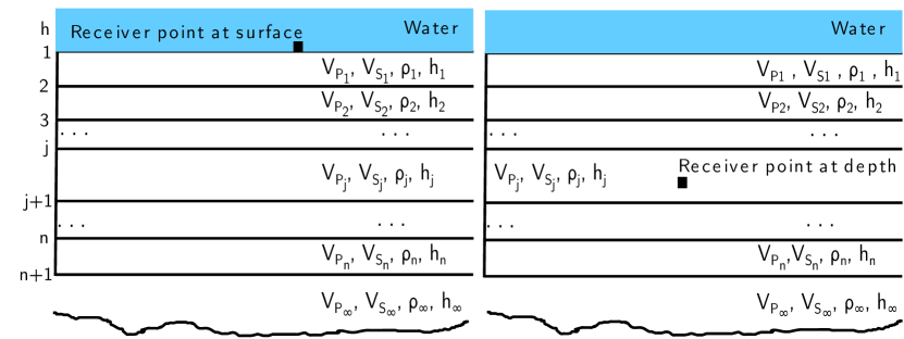
Figure 1: Schematic representation of a 1D layered medium. The representation without the water layer on top corresponds to the onshore case and the representation with water layer corresponds to the offshore case. For the representation on the left, the receiver location is at the earth surface when no water layer is present (onshore) and at the water (lake, sea, ocean) bottom when the water layer is present (offshore). For the representation on the right, the receiver location is at depth. Except for the water layer in the offshore case where the shear wave velocity is zero, any other layer $j$ either onshore or offshore is characterized by the seismic parameters $V_{\text{P}_{j}}$, $V_{\text{S}_{j}}$, $\rho_{j}$, $h_{j}$, $Q_{\text{P}_{j}}$, and $Q_{\text{S}_{j}}$.

Assuming the subsurface structure can be approximated by a stack of homogeneous layers over a half-space as depicted in Figure 1 where for example the $j^{th}$ layer is characterized in the onshore case by the compressional wave velocity $V_{\text{P}_{j}}$ , the shear wave velocity $V_{\text{S}_{j}}$, the density $\rho_{j}$, the layer thickness $h_{j}$, and the attenuation parameters $Q_{\text{P}_{j}}$ and $Q_{\text{S}_{j}}$ for the P- and and S-wave respectively, Im$[G_{11}]$, Im$[G_{22}]$ and Im$[G_{33}]$ are given by:

$$\begin{aligned} \text{Im}[G_{11}]=\frac{1}{4\pi}\int_{0}^{\infty}\text{Im}\left[g_{11\text{SH}}\right]kdk+\frac{1}{4\pi}\int_{0}^{\infty}\text{Im}\left[g_{11\text{PSV}}\right]kdk\end{aligned}$$ (3)

$$\begin{aligned} \text{Im}[G_{33}]=\frac{1}{2\pi}\int_{0}^{\infty}\text{Im}\left[g_{33\text{PSV}}\right]kdk\cdot\end{aligned}$$ (4)

Because of symmetry, $\text{Im}[G_{11}]=\text{Im}[G_{22}]$. Here $k$ is the radial wavenumber. The kernels $g_{11\text{SH}}$, $g_{11\text{PSV}}$ and $g_{33\text{PSV}}$ correspond to the SH and P-SV wave contributions. The explicit dependence of $g_{11\text{SH}}$, $g_{11\text{PSV}}$, and $g_{33\text{PSV}}$ on the Thomson-Haskell propagator matrix (2x2 for SH waves and 4x4 for P-SV waves) for the layered elastic earth model presented in Figure 1 are given in Appendices B and C.

2.3 $H/V(z,f)$ interpretation: Offshore case

In the particular case where the top layer is a perfect homogeneous water layer, the shear wave velocity and shear modulus do not exist (are null). Substituting directly the corresponding properties into the formulae of the 4x4 propagator matrix for P-SV waves (Equations 68-70) leads to a singular matrix. In this limiting case, there is an alternative approach to consider $P$-waves along the water column. A pseudo 4x4 propagator matrix $\mathbf{P}_{\text{pseudo}}$ is defined (Equation 5) and treated as in the onshore case (Herrmann, 2008).

$$\begin{aligned} \mathbf{P}_{\text{pseudo}}&=\begin{pmatrix}1&0&0&0\\ 0&\cosh(\gamma h)&0&-\dfrac{\gamma}{\rho\omega}\sinh(\gamma h)\\ 0&0&1&0\\ 0&-\dfrac{\rho\omega^{2}}{\gamma}\sinh(\gamma h)&0&\cosh(\gamma h)\end{pmatrix}\\ \end{aligned},$$ (5)

where $\gamma=\sqrt{k^{2}-\omega^{2}/V_{\text{P}}^{2}}$ represents the vertical wavenumber for P-wave in water and $h$ the thickness of the water column. A full derivation of $\mathbf{P}_{\text{pseudo}}$ is presented in Appendix E.

2.4 Considerations for numerical implementation

For the numerical integration, equations 3 and 4 are transformed into a summation assuming virtual sources spread along the horizontal plane with generic spacing $L$ (Bouchon & Aki, 1977). The parameter $L$ also defines the integration step $dk=\dfrac{2\pi}{L}$. The vertical wavenumbers $\gamma_{j}$ and $\nu_{j}$ for, respectively, $P-$ and $S-$waves in the $j^{th}$ layer relate to the horizontal wavenumbers $k$ by:

$$\begin{aligned} \gamma_{j}=\sqrt{k^{2}-\frac{\omega^{2}}{V_{\text{P}_{j}}^{2}}}\end{aligned}$$ (6)

$$\begin{aligned} \nu_{j}=\sqrt{k^{2}-\frac{\omega^{2}}{V_{\text{S}_{j}}^{2}}}.\end{aligned}$$ (7)

Because of pole singularities of the kernel that account for the effects of surface waves, a stable integration on the real axis can be performed if a correction term $\omega_{I}$ is added to the frequency to shift the poles of the kernel from the real axis, so that the effective frequency is:

$$\omega=2\pi f+\omega_{I}i,$$ (8)

where $i$ is the unit imaginary number. $\omega_{I}$ is chosen as the smallest constant that effectively smooth out the kernels. Anelastic attenuation of P- and S-wave energy is considered by defining complex seismic wave velocities (See e.g. Müller, 1985).

Additional considerations are made to avoid the loss-of-precision associated with the Thomson-Haskell propagator matrix when waves become evanescent. A numerical procedure is inserted into the matrix propagation loop to make all determined displacement vectors in-situ orthonormal (Wang, 1999). The orthonormalization procedure, as implemented here, for both surface downward- and infinity upward wave propagation of the determined base vectors is presented in Appendix D.

3 Synthetic analysis using canonical and realistic earth models

For testing the presented algorithm, the directional energy density profile for a homogeneous half-space is computed. Table 1 presents the model parameters for this simple earth structure defined as a Poisson solid.

Table 1: Seismic parameters for a homogeneous half-space. The model is used to estimate the directional energy density profile with normalized depth.

$h$ (m)	$V_{P}$ (m/s)	$V_{S}$ (m/s)	$\rho\left(\text{kg/m}^{3}\right)$	$Q_{P}$	$Q_{S}$
$\infty$	1732	1000	2000	100	100

Figure 2: Normalized energy density profiles (Im($G_{11}$), Im($G_{22}$), Im($G_{33})$, and the total directional energy density) for the three orthogonal directions estimated using (1) the algorithm based on the propagator matrix formulation (thin continuous line) and (2) the algorithm based on the global matrix formulation for a layered medium (dashed thick line; Lontsi et al. 2015). The depth is normalized with the Rayleigh wavelength. There is a good agreement between the two approaches for Green’s functions estimation. Input parameters used in the modeling are defined in Table 1.

The energy variation with depth as depicted in Figure 2 shows a good agreement with the known theory regarding the energy partition for a diffuse wavefield (e.g. Weaver, 1985; Perton et al., 2009). For depths larger than approximately 1.5 times the Rayleigh wavelength, there is almost no surface wave energy contribution and the energy is equal for the three orthogonal directions (Figure 2).

Further tests are performed by considering a simple one layer over a half-space (1LOH) and a realistic subsurface structure. The realistic earth model has been obtained from site characterization at Baar, Canton Zug, Switzerland (Hobiger et al., 2016). The parameters for the simple one layer over a half-space model together with those of the realistic earth structure used in the second test are presented in Table 2. The 1LOH structural model represents a very simple soft-soil characterized by a constant shear wave velocity ($V_{S}$) of $200$ m/s, a velocity contrast of $5$ in $V_{S}$ and an overall sediment cover of $25$ m. The realistic earth model at Baar has velocity contrast in $V_{S}$ of about $4$ between the sediment layer overlaying the half-space and the half-space. Here, the overall sediment cover is about $100$ m. In comparison to $V_{S}$ values that remain almost constant, water saturated sediment offshore have compressional wave velocities estimates that are much larger than the onshore values.

Figure 3a, and respectively Figure 4a present the seismic velocity profiles ($V_{P}$ and $V_{S}$) for the two investigated structural models. Considered $V_{P}$ profiles for the water saturated sediments are represented by the blue solid line. The corresponding $H/V(z,f)$ spectral ratio without a water layer (onshore) and with water layer (offshore) are plotted together for different depths. This representation allows for a visual appraisal of the effect of the water column (Figures 3 b-d and 4 b-d).

Table 2: Test models consisting of one and three solid layers over a half-space (onshore). Offshore cases, characterized by $V_{S}=0$ m/s are built by considering a water layer on top. In the case where the water layer is considered, the $V_{P}$ velocities for the sediment at the bottom of the water column are modified to account for the saturation with water. Considered values for $V_{P}$ are shown in parenthesis in the appropriated column. Scenarios for different water environments ranging from shallow to deep are considered. The $H/V$ spectral ratios at three different locations (surface + two additional depths) for these two illustrative cases are presented in Figures 3 and 4.

One-layer over a half-space
$h$ (m)	$V_{P}$ (m/s)	$V_{S}$ (m/s)	$\rho\left(\text{kg/m}^{3}\right)$	$Q_{P}$	$Q_{S}$
8a(200b,5000c)	1500	0	1000	99999	99999
25	500 (1700)	200	1900	100	100
$\infty$	2000	1000	2500	200	200
Realistic earth model at Baar, Canton Zug
8a(200b,5000c)	1500	0	1000	99999	99999
5.3	672.8 (1600)	85.6	2000	100	100
29.2	738.9 (1600)	284.3	2000	100	100
68.4	2135.6	500.0	2000	100	100
$\infty$	3512.2	1841.1	2300	100	100

^a Thin water layer. ^b Lake environment. ^c Deep ocean environment.

Figure 3: a) Seismic parameters for a simple soft soil layer over a half-space (defined in Table 2). The P-wave velocity in water is set to $1500$ m/s. The water-saturated sediments have the velocity set to $1700$ m/s (see solid blue profile). The shear-wave velocity ($V_{S}$) profile is set unchanged in the presence of the water layer. b) Comparison between $H/V$ spectral ratios at the solid-liquid interface ($z=0$ m). c) Comparison between $H/V$ spectral ratios at $19$ m depth and d) at $25$ m depth. The gray curve is obtained using the extended global matrix formulation for receivers at depth when no water layer is present (see Lontsi et al. 2015). The computed $H/V$ for a synthetic water layer of $200$ and $5000$ m shows nearly the same results and are almost overlayed with each other; see green and red curves.

Figure 4: a) Seismic parameters for a realistic earth model (defined in Table 2. The P-wave velocity for water is set to $1500$ m/s. The P-wave velocity for water-saturated sediments are represented with the solid blue profile. The shear-wave velocity ($V_{S}$) profile is set unchanged in the presence of the water layer. In addition, a sedimentary environment with a very shallow water table is considered. The $V_{P}$ for the sediment in this onshore case was set to $1600$ m/s. b) Comparison between $H/V$ spectral ratios at the solid-free surface and solid-liquid interface ($z=0$ m). For the solid-free surface interface (onshore), field data exist and are used for validation of the presented algorithm (solid gray curve). Frequencies above $8$ Hz (light gray box) were not used for the profile estimation. c) Comparison between $H/V$ spectral ratios at $5.3$ m within the sediment column and d) at $102.9$ m depth (sediment bedrock interface).

The $H/V(z,f)$ spectral ratio computed with the propagator matrix algorithm for the 1LOH are calibrated with results obtained using the global matrix formulation approach as presented by Lontsi et al., 2015 for receivers at depth when no water layer is present (compare solid gray and dashed black dashed lines on Figures 3 b-d). The two approaches (propagator matrix and global matrix formulations) provide $H/V$ spectral ratios that agree with each other for all tested receivers locations for the onshore case.

The presented algorithm is further used to assess the variations of the $H/V$ spectral ratios, at the surface and at depth, due to the presence of the water layer. To this end, the structural models presented in Table 2 with three different water-layer thicknesses ($8$, $200$, $5000$ m) are used. The water layer thicknesses are selected to reflect different water environments ranging from shallow lake to deep sea. For the one layer-over-halspace (1LOH) structural model and for a scenario of shallow water environment with $8$ m water column, we observe at frequencies above $2$ Hz (peak frequency) an amplitude variation. Further scenarios with moderate ($200$ m) to deep ($5000$ m) water layer indicate that the amplitude variations extend to low frequencies and reach up to $50\%$ around the $H/V$ spectral ratio peak amplitude for the receiver at the surface. Only marginal relative variations are observed for the H/V peak frequency when the water layer is present. The amplitude variation as well as the marginal peak frequency variation observed for the one layer-over-halspace in different water environments are also valid for the realistic earth model at Baar. For this particular test site, we further consider that the water table is very shallow and investigate the onshore scenario with water saturated sediments cover. The $V_{P}$ velocity for the first two layers was set to $V_{P}=1600$ m/s to consider the saturation with water. The resulting H/V spectral ratio computed at different depths indicates that changes in Vp do have influence on the shape of the H/V spectral ratio in the frequency band ranging from about 1 to 3 Hz for receivers at the surface and at depths, although very minor (see Figure 4b-d). At Baar, onshore ambient vibrations data from array recordings are available. The surface waves analysis allowed to extract the average seismic velocity profiles of the underlying subsurface structure (for more details, see Hobiger et al. 2016). The estimated velocity profiles did not account for $H/V$ information beyond $8$ Hz shown in the light gray box (Figure 4b). The $H/V$ spectral ratio from the array central station is used for calibration (gray curve in Figure 4b).

Within the sediment column, and for all considered water column thicknesses, the variability of the $H/V$ spectral ratio is observed up to a certain cut-off frequency. This cut-off frequency is about $5$ Hz at $19$ m depth for the 1LOH structural model. For the realistic earth model at Baar and for a receiver at about $5.3$ m depth, the cut-off frequency is about $10$ Hz. In the last case where the receiver is located at the bedrock interface, a marginal $H/V$ amplitude variations are observed (Figures 3d and 4d). For both models, the low-frequency peak corresponds well with the fundamental resonance of SH waves in the structure. In the case of the layer above the half-space it is given by the simple relationship $f_{0}=\dfrac{V_{S}}{4H}$, where $H$ is the thickness of the sediment column and $V_{S}$ is the shear wave velocity ($Vs=200$ m/s and $H=25$ m, Figure 3a). For the realistic model at Baar (Figure 4a), the peak frequency can be estimated by using the simple expression found by Tuan et al. (2016) with about $10\%$ deviation. Secondary peaks for the simple one layer over a half-space (Figure 3a) satisfy the relationship $f_{n}=\dfrac{V_{S}}{4H}(2n+1)$. For the realistic earth model at Baar (Figure 4), the second dominant peak at about $4$ Hz corresponds to the response of the top layer characterized by a shear wave velocity $Vs=85$ m/s. The corresponding impedance contrast is about $3.34$. A weak impedance contrast of about $1.76$ exists between the second and third layer. Additional peaks (Gray box Figure 4 b) would depend on very shallow features not represented by the considered velocity model.

4 Understanding the $H/V$ amplitude variation

The observed amplitude variation of the H/V in the presence of the water layer are investigated by analyzing the modeled directional energy densities (DED) both on the horizontal and vertical components. The earth model at Baar is used for the analysis. Figures 5 and 6 show the modeled DED for the horizontal and vertical components respectively. Considered scenarios include an earth model (1) without water layer, (2) with no water layer but very shallow water table, (3) with water layer with 8-, 200-, and 5000 m. It comes out that the energy on the horizontal component is not sensitive to the presence of the water layer. This is understood as no shear wave is expected to propagate in the considered ideal fluid (no viscosity). On the contrary, we observe significant energy variations on the vertical component that can be associated with multiple energy reverberations in the water layer.

Figure 5: Horizontal directional energy density variation at the seabottom using the structural earth model at Baar. Different water layer thicknesses are considered.

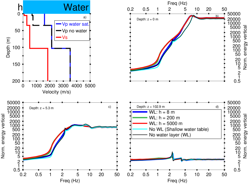
Figure 6: Vertical directional energy density variation at the seabottom using the structural earth model at Baar. Different water layer thicknesses are considered.

We further assess the dependence of the amplitude variation with a much larger number of water layer thicknesses scenario. For this purpose, the relative variation of H/V spectral ratio when there is water layer is studied. Figure 7 depicts this relative variations in percent for a wide range of water columns. It can be observed that the presence of a shallow water layer mainly has effects on the very high frequency. Deep water environment affect the amplitude of the H/V spectral ratio on a very broad frequency range.

Figure 7: Relative variation of the H/V spectral ratio in the presence of the water layer with respect the the H/V spectral ratio when no water layer is present. Water layer thicknesses ranging between 0.1 and 5000 m, sampled on a logarithmic scale are considered. Left: One layer over half-space structure. Right: Realistic earth model at Baar.

5 Conclusions

A theoretical model based on the diffuse field approximation is proposed for the estimation of the horizontal-to-vertical ($H/V(z,f)$) spectral ratio on land and in marine environment. The propagator matrix (PM) method has been used to compute the Green’s function in a 1D layered medium including a liquid layer atop. For onshore cases, the modeled $H/V(z,f)$ spectral curves are compared with estimations from the global matrix (GM) approach and show good agreement for the considered synthetic structural models. In comparison to the GM method, the PM provides an efficient approach for modeling the $H/V$ spectral ratio within marine environments. Modeling results indicate that the $H/V$ spectral ratio is sensitive to the presence of a water layer overlying subseabed sediments. $H/V$ relative amplitude variations are observed in the complete considered frequency range ($0.2-50$ Hz) for deep water environment and may reach approximately $50\%$ around the peak frequency. The amplitude decrease in the $H/V$ peak can be understood as large P-wave energy on the vertical component result from multiple reverberation in the water column. The $H/V$ data available at Baar (onshore) are used to validate the presented algorithm for a receiver at the surface. For computed cases, changes in the fundamental frequency are marginal. In addition, primary resonances occur at frequencies that satisfy the relationships used in practical applications. Secondary resonances in the 1LOH corresponds to overtones while in the realistic case at Baar, they materialize the response of the subsequent layers within the sediment column.

Appendix A Ambient noise - Green’s function - representation theorem - cross-correlation - Directional Energy Density - Equipartition

Seismic sources at the origin of the ambient noise wavefield are ubiquitous and may be at surface or/and at depth. Generated seismic waves are back-scattered in the subsurface. The recorded noise wavefield at a seismic station after a lapse time large enough compared to the mean travel time of ballistic waves (e.g direct waves, first reflected waves) contains information regarding the underlying subsurface structure.

Let us assume that there is an asymptotic regime with a stable supply of energy that constitutes the background illumination. This condition, for what it shares with the radiative transport, is called diffuse field. In an unbounded elastic medium a harmonic diffuse field is considered random, isotropic and equipartitioned. The stabilization of the S to P energy ratio is reached asymptotically for long lapse times (Paul et al., 2005). Within such a field the Directional Energy Density (DED), $E_{m}$, for a given orthogonal direction $m$ is given in terms of the averaged autocorrelation of the displacement wavefield and it is proportional to the imaginary part of the Green’s function of the system for the source and the receiver at the same location. This is expressed in Equation 9:

$$\begin{aligned} E_{m}(\mathbf{x},f)=\rho\omega^{2}\langle u_{m}(\mathbf{x},f)u_{m}^{*}(\mathbf{x},f)\rangle\propto\text{Im}[G_{mm}(\mathbf{x},\mathbf{x},f)]\end{aligned}$$ (9)

Here $\rho=\rho(\mathbf{x})$ is the mass density at point $\mathbf{x}$, and $\omega=2\pi f$ is the circular frequency. No summation over the repeated index $m$ is assumed. In practice, the DED is estimated from the autocorrelation (power spectrum) of the recorded ambient noise wavefield and averaged over short time windows. This is equivalent to average over directions if the field is isotropic. For subsurface imaging purposes, the DED is computed from the imaginary part of the Green’s function (Equation 9).

In order to demonstrate the validity of Equation 9 and establish the proportionality factor, a simple homogeneous, isotropic, elastic medium is considered. Therefore, the analytical expression to the Green’s function is known (Sánchez-Sesma et al., 2008).

The displacement field $u_{i}(\mathbf{x},\omega)$ produced by a body force $f_{i}$ at a given point $\mathbf{x}$ of an elastic solid is described by the Newton’s law of displacements (Equation 10).

$$\dfrac{\partial}{\partial x_{j}}\left(c_{ijkl}\dfrac{\partial u_{l}(\mathbf{x},\omega)}{\partial x_{k}}\right)+\omega^{2}\rho u_{i}(\mathbf{x},\omega)=-f_{i}(\mathbf{x},\omega)$$ (10)

Equation 10 is often called elastic wave equation or Navier equation. Here $c_{ijkl}$ is the stiffness tensor. The Einstein summation convention is assumed, i.e repeated index implies summation over the range of that index.

From Equation 10, it is possible to derive the classical Somigliana representation theorem (e.g. Wapenaar & Fokkema, 2006; van Manen et al., 2006; Snieder et al., 2007; Sánchez-Sesma et al., 2008, 2018):

$$\begin{aligned} &u_{m}(\mathbf{x_{A}},\omega)=\\ &\int_{\varGamma}\left[G_{im}(\mathbf{x},\mathbf{x_{A}},\omega)t_{i}(\mathbf{x},\omega)-T_{im}(\mathbf{x},\mathbf{x_{A}},\omega)u_{i}(\mathbf{x},\omega)\right]d\varGamma_{x}+\int_{V}f_{i}(\mathbf{x},\omega)G_{im}(\mathbf{x_{A}},\mathbf{x},\omega)dV_{x}\end{aligned}$$ (11)

in which one has the displacement field for $\mathbf{x_{A}}$ being a point at $V$ inside the surface $\varGamma$ in terms of body forces and the boundary values of displacements and tractions. Here $G_{im}(\mathbf{x_{A}},\mathbf{x},\omega)$ and $T_{im}(\mathbf{x_{A}},\mathbf{x},\omega)$ are the Green’s functions for displacements and tractions when the harmonic unit force are in the direction $m$. $f_{i}(\mathbf{x})$ is the body force distribution. $t_{i}(\mathbf{x},\omega)$ and $T_{im}(\mathbf{x_{A}},\mathbf{x},\omega)$ are defined by Equation 12.

$$\begin{aligned} &t_{i}(\mathbf{x},\omega)=n_{j}(\mathbf{x})\left(c_{ijkl}\dfrac{\partial u_{l}(\mathbf{x},\omega)}{\partial x_{k}}\right)\\ &T_{im}(\mathbf{x_{A}},\mathbf{x},\omega)=n_{j}(\mathbf{x})\left(c_{ijkl}\dfrac{\partial G_{lm}(\mathbf{x},\mathbf{x_{A}},\omega)}{\partial x_{k}}\right)\cdot\end{aligned}$$ (12)

By considering for the internal point $\mathbf{x_{B}}$ an harmonic body force $f_{i}(\mathbf{x})\equiv\delta(\mathbf{x}-\mathbf{x_{B}})\delta_{in}$ in the direction $n$ and setting for the field the time-reversed solution, then $u_{i}(\mathbf{x})\equiv G_{in}(\mathbf{x},\mathbf{x_{B}},\omega)$, $t_{i}(\mathbf{x})\equiv T_{in}(\mathbf{x},\mathbf{x_{B}},\omega)$, and Equation 11 becomes:

$$\begin{aligned} &\int_{\varGamma}\left[T_{im}(\mathbf{x},\mathbf{x_{A}},\omega)G_{in}^{*}(\mathbf{x},\mathbf{x_{B}},\omega)-T_{in}^{*}(\mathbf{x},\mathbf{x_{B}},\omega)G_{im}(\mathbf{x},\mathbf{x_{A}},\omega)\right]d\varGamma_{x}=\\ &-G_{mn}^{*}(\mathbf{x_{A}},\mathbf{x_{B}},\omega)+G_{mn}(\mathbf{x_{A}},\mathbf{x_{B}},\omega)\end{aligned}$$ (13)

which is re-written changing $\mathbf{x}$ by $\mathbf{\xi}$, to represent boundary points on $\varGamma$, as:

$$\begin{aligned} &2\mathbf{i}G_{mn}(\mathbf{x_{A}},\mathbf{x_{B}},\omega)=\\ &-\int_{\varGamma}\left[G_{mi}(\mathbf{x_{A}},\mathbf{\xi},\omega)T_{in}^{*}(\mathbf{\xi},\mathbf{x_{B}},\omega)-G_{ni}^{*}(\mathbf{x_{B}},\mathbf{\xi},\omega)T_{im}(\mathbf{\xi},\mathbf{x_{A}},\omega)\right]d\varGamma_{\xi}\cdot\end{aligned}$$ (14)

The Equation 14 is a correlation-type representation theorem. A similar form has been presented by van Manen et al. (2006). Then because the theorem in Equation 14 is valid for any surface $\varGamma$, it follows that if the field is diffuse at the envelope,i.e. the net flux of energy is null, it is also diffuse at any point within the heterogeneous medium

Starting from the analytical expressions for $G_{im}$ and $T_{im}$ in the farfield (Sánchez-Sesma & Campillo, 2006; Sánchez-Sesma et al., 2008; see, e.g., Domínguez & Abascal, 1984 for the full expression of $G_{im}$ and $T_{im}$), it can be demonstrated, that for random and uncorrelated sources, the resulting illumination, after a lapse time large enough compared to the travel time of ballistic waves, is an equipartitioned diffuse field. Therefore, the right hand side of equation 14 is proportional to the azimuthal average of crosscorrelation of the displacement field.

$$\begin{aligned} \text{Im}[G_{mn}(\mathbf{x_{A}},\mathbf{x_{B}})]=-(2\pi\xi_{S})^{-1}k^{3}\langle u_{m}(\mathbf{x_{A}})u_{n}^{*}(\mathbf{x_{B}})\rangle\end{aligned}$$ (15)

Where $k$ is the shear wave number and $\xi_{S}$ is the average energy density of shear waves and represents a measure of the strength of the diffuse illumination. Assuming the source and the receiver are at the same location ($\mathbf{x_{A}}=\mathbf{x_{B}}=\mathbf{x}$), one can thus write (Sánchez-Sesma et al., 2008):

$$\begin{aligned} \text{Im}[G_{mm}(\mathbf{x},\mathbf{x})]=-(2\pi\xi_{S})^{-1}k^{3}\langle|u_{m}(\mathbf{x})|^{2}\rangle\end{aligned}$$ (16)

An alternative approach linking the azimuthal average of cross-correlation to the imaginary part of the Green’s function under diffuse assumption in the farfield, and without prior knowledge of the full analytical expression of the Green’s function was presented by Snieder et al. (2009).

Appendix B Estimating the SH waves contribution to the imaginary part of the Green’s function

B.1 Receiver at the surface

Following Aki & Richards, 2002, and for the displacement $u_{2}=v$, the SH-wave equation in an arbitrary layer $j$ presented in Figure 1 is given in linear elasticity by:

$$\dfrac{\partial^{2}v}{\partial t^{2}}=\dfrac{\mu_{j}}{\rho_{j}}\left(\dfrac{\partial^{2}v}{\partial x^{2}}+\dfrac{\partial^{2}v}{\partial z^{2}}\right)$$ (17)

A solution to the Equation 17 can be of the form:

$$v=l_{1}(z,w,k)\exp[i(kx-\omega t)]$$ (18)

and the associated shear stresses:

$$\begin{aligned} \tau_{yz}&=\mu_{j}\dfrac{\partial l_{1}}{\partial z}\exp[i(kx-\omega t)]\\ &=l_{2}\exp[i(kx-\omega t)]\\ \tau_{xy}&=ik\mu_{j}l_{1}\exp[i(kx-\omega t)]\cdot\end{aligned}$$ (19)

From Equation 19, the differential Equation 20 is obtained.

$$\dfrac{dl_{1}}{dz}=\dfrac{1}{\mu_{j}}l_{2}$$ (20)

From Newton’s second law, one gets:

$$\dfrac{\partial\tau_{xy}}{\partial x}+\dfrac{\partial\tau_{yz}}{\partial z}=\rho_{j}\dfrac{\partial^{2}v}{\partial t^{2}}$$ (21)

This leads to

$$\dfrac{dl_{2}}{dz}=(k^{2}\mu_{j}-\omega^{2}\rho_{j})l_{1}$$ (22)

Equations 20 and 22 lead to the system of first order differential equations 23.

$$\dfrac{d}{dz}\dbinom{l_{1}}{l_{2}}=\begin{pmatrix}0&\dfrac{1}{\mu_{j}}\\ k^{2}\mu_{j}-\omega^{2}\rho_{j}&0\\ \end{pmatrix}\dbinom{l_{1}}{l_{2}}$$ (23)

This equation is of the form:

$$\dfrac{d\mathbf{l}}{dz}=\mathbf{A}_{j}\mathbf{l}$$ (24)

where

$$\mathbf{l}=\dbinom{l_{1}}{l_{2}}$$ (25)

and

$$\mathbf{A}_{j}=\begin{pmatrix}0&\dfrac{1}{\mu_{j}}\\ k^{2}\mu_{j}-\omega^{2}\rho_{j}&0\end{pmatrix}\cdot$$ (26)

Assuming a homogeneous layer medium (i.e., the layers properties are constant), the solution to Equation 24 within the $j^{th}$ layer defined by $z_{j}$ and $z_{j+1}$ is given by:

$$\dbinom{l_{1}}{l_{2}}_{z_{j+1}}=\mathbf{P}_{j}\dbinom{l_{1}}{l_{2}}_{z_{j}}$$ (27)

where

$$\mathbf{P}_{j}=\exp[\mathbf{A}_{j}(z_{j+1}-z_{j})]$$ (28)

Using linear algebra properties, it can be shown that if the matrix $\mathbf{A}$ is diagonalizable, then there exists an invertible $\mathbf{L}$ so that

$$\mathbf{A}=\mathbf{LeL}^{-1}$$ (29)

where $\mathbf{L}$ is the matrix of eigenvectors of $\mathbf{A}$; $\mathbf{L}^{-1}$ its inverse, and $\mathbf{e}$ is the eigenvalue matrix. The series expansion of $\exp[\mathbf{A}(z_{j+1}-z_{j})]$ using

$$\exp(\mathbf{A})=\sum_{k=0}^{\infty}\dfrac{\mathbf{A}^{k}}{k!}=\mathbf{I}+\mathbf{A}+\dfrac{\mathbf{A}^{2}}{2!}+\dfrac{\mathbf{A}^{3}}{3!}+\cdots$$ (30)

allows to write:

$$\exp(\mathbf{L}^{-1}\mathbf{AL})=\exp(\mathbf{e})=\mathbf{E}=\mathbf{L}^{-1}\left(\mathbf{I}+\mathbf{A}+\dfrac{\mathbf{A}^{2}}{2!}+\dfrac{\mathbf{A}^{3}}{3!}+\ldots\right)\mathbf{L}=\mathbf{L}^{-1}[\exp(\mathbf{A})]\mathbf{L}$$ (31)

Where $\mathbf{E}=\exp(\mathbf{e})$. For the problem investigated, $\mathbf{A}$ is replaced by $\mathbf{A}_{j}(z_{j+1}-z_{j})$.

The eigenvalues for the 2x2 $\mathbf{A}(z_{j+1}-z_{j})$ for the SH wave propagation are obtained by finding the roots of the second order polynomial defined by:

$$\det[\mathbf{A}_{j}(z_{j+1}-z_{j})-\lambda I]=0$$ (32)

This leads to

$$\lambda_{1}=(z_{j+1}-z_{j})\nu_{j}$$ (33)

$$\lambda_{2}=-(z_{j+1}-z_{j})\nu_{j}$$ (34)

where $\nu_{j}=\sqrt{k^{2}-\dfrac{\omega^{2}\rho_{j}}{\mu_{j}}}=\sqrt{k^{2}-\dfrac{\omega^{2}}{V_{S_{j}}^{2}}}$

The eigenvectors are obtained by solving the equations (for the two eigenvalues):

$$[\mathbf{A}_{j}(z_{j+1}-z_{j})-\lambda_{1}I]\begin{pmatrix}x_{1}\\ x_{2}\end{pmatrix}=0$$ (35)

and

$$[\mathbf{A}_{j}(z_{j+1}-z_{j})-\lambda_{2}I]\begin{pmatrix}x_{1}\\ x_{2}\end{pmatrix}=0$$ (36)

Sample eigenvectors are therefore:

for $\lambda_{1}$:

$$(x_{1},x_{2})=(1,\mu_{j}\nu_{j})x_{1}$$ (37)

and for $\lambda_{2}$:

$$(x_{1},x_{2})=(1,-\mu_{j}\nu_{j})x_{1}\cdot$$ (38)

The eigenvectors can be arranged in the matrix

$$\mathbf{L}_{j}=\begin{pmatrix}1&1\\ \mu_{j}\nu_{j}&-\mu_{j}\nu_{j}\end{pmatrix}$$ (39)

and the inverse of $\mathbf{L}_{j}$ is given by:

$$\mathbf{L}_{j}^{-1}=\begin{pmatrix}\dfrac{1}{2}&\dfrac{1}{2\mu_{j}\nu_{j}}\\ \dfrac{1}{2}&\dfrac{-1}{2\mu_{j}\nu_{j}}\end{pmatrix}$$ (40)

The matrix $\mathbf{E}_{j}$ is given by:

$$\mathbf{E}_{j}=\begin{pmatrix}\exp[\nu_{j}(z_{j+1}-z_{j})]&0\\ 0&\exp[-\nu_{j}(z_{j+1}-z_{j})]\end{pmatrix}$$ (41)

The eigenvalue problem has also been studied by Gantmacher, 1959; Gilbert & Backus, 1966.

The propagator (or layer) matrix can therefore be written as:

$$\begin{aligned} \mathbf{P}_{j}&=\mathbf{L}_{j}\mathbf{E}_{j}\mathbf{L}_{j}^{-1}\\ &=\begin{pmatrix}1&1\\ \mu_{j}\nu_{j}&-\mu_{j}\nu_{j}\end{pmatrix}\begin{pmatrix}\exp[\nu_{j}(z_{j+1}-z_{j})]&0\\ 0&\exp[-\nu_{j}(z_{j+1}-z_{j})]\end{pmatrix}\begin{pmatrix}\dfrac{1}{2}&\dfrac{1}{2\mu_{j}\nu_{j}}\\ \dfrac{1}{2}&\dfrac{-1}{2\mu_{j}\nu_{j}}\end{pmatrix}\end{aligned}$$ (42)

This operation leads to

$$\mathbf{P}_{j}=\begin{pmatrix}\cosh[\nu_{j}(z_{j+1}-z_{j})]&\dfrac{1}{\mu_{j}\nu_{j}}\sinh[\nu_{j}(z_{j+1}-z_{j})]\\ \mu_{j}\nu_{j}\sinh[\nu_{j}(z_{j+1}-z_{j})]&\cosh[\nu_{j}(z_{j+1}-z_{j})]\end{pmatrix}$$ (43)

In the next steps, the propagator matrix as defined by Equation 42 is used. This representation allows to introduce a manipulation matrix to avoid the instability problem in the high frequency range.

For a $n$-layer over half-space system, we obtain:

$$\dbinom{l_{1}}{l_{2}}_{z_{n+1}}=\mathbf{P}_{n}\mathbf{P}_{n-1}...\mathbf{P}_{1}\dbinom{l_{1}}{l_{2}}_{z_{1}}$$ (44)

By introducing Equation 18 into Equation 21, a second order differential equation is obtained for $l_{1}$ where the solution can be written for layer 1 in the form:

$$l_{1}=\acute{S}_{1}\exp(\nu_{1}z)+\grave{S}_{1}\exp(-\nu_{1}z)$$ (45)

where $\acute{S}_{1}$ and $\grave{S}_{1}$ are constant representing the amplitude of upgoing- and downgoing SH waves.
Equations 20 and 45 lead to

$$l_{2}=\mu_{1}\nu_{1}\acute{S}_{1}\exp(\nu_{1}z)-\mu_{1}\nu_{1}\grave{S}_{1}\exp(-\nu_{1}z)$$ (46)

Equation 45 and 46 combine to

$$\dbinom{l_{1}}{l_{2}}=\begin{pmatrix}\exp(\nu_{1}z)&\exp(-\nu_{1}z)\\ \mu_{1}\nu_{1}\exp(\nu_{1}z)&-\mu_{1}\nu_{1}\exp(-\nu_{1}z)\end{pmatrix}\dbinom{\acute{S}_{1}}{\grave{S}_{1}}$$ (47)

Without loss of generality, we have for the half-space:

$$\begin{aligned} \dbinom{l_{1}}{l_{2}}_{n+1}&=\begin{pmatrix}\exp(\nu_{n+1}z)&\exp(-\nu_{n+1}z)\\ \mu_{n+1}\nu_{n+1}\exp(\nu_{n+1}z)&-\mu_{n+1}\nu_{n+1}\exp(-\nu_{n+1}z)\end{pmatrix}\dbinom{\acute{S}_{n+1}}{\grave{S}_{n+1}}\\ &=\begin{pmatrix}1&1\\ \mu_{n+1}\nu_{n+1}&-\mu_{n+1}\nu_{n+1}\end{pmatrix}\dbinom{\acute{S}_{1}\exp(\nu_{n+1}z)}{\grave{S}_{1}\exp(-\nu_{n+1}z)}\\ &=\mathbf{L}_{n+1}\dbinom{\acute{S}_{n+1}\exp(\nu_{n+1}z)}{\grave{S}_{n+1}\exp(-\nu_{n+1}z)}\\ &=\mathbf{L}_{n+1}\begin{pmatrix}\exp(\nu_{n+1}z_{n+1})&0\\ 0&\exp(-\nu_{n+1}z_{n+1})\end{pmatrix}\dbinom{\acute{S}_{n+1}}{\grave{S}_{n+1}}\end{aligned}$$ (48)

In the half-space, there is no up-going waves, therefore $\acute{S}_{n+1}=0$, so that:

$$\begin{aligned} \dbinom{l_{1}}{l_{2}}_{n+1}&=\mathbf{L}_{n+1}\begin{pmatrix}\exp(\nu_{n+1}z_{n+1})&0\\ 0&\exp(-\nu_{n+1}z_{n+1})\end{pmatrix}\dbinom{0}{\grave{S}_{n+1}}\\ &=\mathbf{L}_{n+1}\begin{pmatrix}\exp(\nu_{n+1}z_{n+1})&0\\ 0&\exp(-\nu_{n+1}z_{n+1})\end{pmatrix}\dbinom{0}{1}\grave{S}_{n+1}\end{aligned}$$ (49)

Using Equation 42, 44, and 49, we have:

$$\mathbf{P}_{n}\mathbf{P}_{n-1}...\mathbf{P}_{1}\dbinom{l_{1}}{l_{2}}_{1}=\mathbf{L}_{n+1}\begin{pmatrix}\exp(\nu_{n+1}z_{n+1})&0\\ 0&\exp(-\nu_{n+1}z_{n+1})\end{pmatrix}\dbinom{0}{1}\grave{S}_{n+1}$$ (50)

This leads, for the displacement at the surface to:

$$\dbinom{l_{1}}{l_{2}}_{1} =\mathbf{P}_{1}^{-1}...\mathbf{P}_{n-1}^{-1}\mathbf{P}_{n}^{-1}\mathbf{L}_{n+1}\dbinom{0}{1}\grave{S}_{n+1}\exp(-\nu_{n+1}z_{n+1})$$ (51)

Where $\mathbf{P}_{n}^{-1}=\mathbf{L}_{n}\mathbf{E}_{n}^{-1}\mathbf{L}_{n}^{-1}$

Lets set $\mathbf{C}_{n+1}=\dbinom{0}{1}$ and $\mathbf{Y}_{n+1}=\mathbf{L}_{n+1}\mathbf{C}_{n+1}$

At the surface load point ($z=0$), $l_{1}=v=g_{22\text{SH}}$ (the integrand of interest) and $l_{2}=1$.

Equation 51 can be solved for $g_{22\text{SH}}$ at the surface.

The Green’s function in the 1D layered medium is obtained by integration over the horizontal wavenumber:

$$\text{Im}\left[G_{22}^{SH}(z,f)\right]=\text{Im}\left[G_{11}^{SH}(z,f)\right]=\frac{1}{4\pi}\int_{0}^{\infty}\text{Im}\left[g_{22\text{SH}}\right]kdk$$ (52)

Note that a correction factor $\dfrac{k}{4\pi}$ has been introduced in the kernel. This is trivial in cylindrical coordinates when the radius and azimuthal components are set to zero.

B.2 Receiver at depth

For a receiver at depth, the displacement-stress just under the load point which is assumed to be at the interface $j$ can be written as follows (compare Equation 51):

$$\begin{aligned} \dbinom{l_{b1}}{l_{b2}}_{z_{j}}=\mathbf{P}_{j}^{-1}...\mathbf{P}_{n-1}^{-1}\mathbf{P}_{n}^{-1}\mathbf{L}_{n+1}\dbinom{0}{1}\grave{S}_{n+1}\exp(-\nu_{n+1}z_{n+1})\end{aligned}$$ (53)

On the other hand, the result just above the source would be:

$$\begin{aligned} \dbinom{l_{u1}}{l_{u2}}_{z_{j}}=\mathbf{P}_{j-1}\mathbf{P}_{j-2}...\mathbf{P}_{1}\dbinom{l_{1}}{l_{2}}_{z_{1}}\end{aligned}$$ (54)

.

The boundary conditions at the load point at depth are given (1) for the upper layer by $l_{u1}$ = $g_{22\text{SH}}$; and $l_{u2}$ = $\tau_{u}$ and (2) for the bottom layers by: $l_{b1}$ = $g_{22\text{SH}}$ and $l_{b2}$ = $\tau_{b}$. The unit load at the source is defined such that $\tau_{b}-\tau_{u}=1$

Equation 54 can be rewritten as

$$\begin{aligned} \dbinom{l_{u1}}{l_{u2}}_{z_{j}}&=\mathbf{P}_{j-1}\mathbf{P}_{j-2}...\mathbf{P}_{1}\dbinom{v_{s}}{0}_{z_{1}}\\ &=\mathbf{P}_{j-1}\mathbf{P}_{j-2}...\mathbf{P}_{1}\dbinom{1}{0}v_{s}\end{aligned}$$ (55)

Lets set $\mathbf{Y}_{1}=\dbinom{1}{0}$ as the basic displacement-stress solution at the surface. This basic vector is propagated downwards from the surface to the source. So that:

$$\dbinom{Y_{u1}}{Y_{u2}}=\mathbf{P}_{j-1}\mathbf{P}_{j-2}...\mathbf{P}_{1}\dbinom{1}{0}\cdot$$ (56)

Respectively, the fundamental vector of plane-wave amplitude $\dbinom{0}{1}$ at the half-space can be propagated upwards to the source:

$$\dbinom{Y_{b1}}{Y_{b2}}=\mathbf{P}_{j}^{-1}...\mathbf{P}_{n-1}^{-1}\mathbf{P}_{n}^{-1}\mathbf{L}_{n+1}\dbinom{0}{1}$$ (57)

The set of boundary conditions allows to extract $g_{22\text{SH}}$ as:

$$g_{22\text{SH}}=\frac{Y_{u1}Y_{b1}}{Y_{u1}Y_{b2}-Y_{u2}Y_{b1}}$$ (58)

For this SH case, the Green’s function in the 1D layered medium is given by:

$$\text{Im}\left[G_{22}^{SH}(z,f)\right]=\text{Im}\left[G_{11}^{SH}(z,f)\right]=\frac{1}{4\pi}\int_{0}^{\infty}\text{Im}\left[g_{22\text{SH}}\right]kdk$$ (59)

The integral can be numerically computed by making, e.g., use of the discrete wavenumber approach.

Appendix C Computing the P-SV waves contribution to the imaginary part of the Green’s function

Without loss of generality, consider the inplane solution ( i.e. no dependence on the $y$ coordinate) to the elastic wave or Navier equation. The displacement-stress vector $\mathbf{r}=(r_{1},r_{2},r_{3},r_{4})^{T}$ is obtained by the following expression (see also e.g. Aki & Richards, 2002; Chap7, p263):

$$\begin{aligned} u&=r_{1}(k,z,\omega)\exp[i(kx-\omega t)],\\ v&=0,\\ w&=ir_{2}(k,z,\omega)\exp[i(kx-\omega t)],\end{aligned}$$ (60)

Here we used $(u_{1},u_{2},u_{3})=(u,v,w)$. Let set the stresses associated to displacements:

$$\begin{aligned} \tau_{zx}&=r_{3}(k,z,\omega)\exp[i(kx-\omega t)],\\ \tau_{zz}&=ir_{4}(k,z,\omega)\exp[i(kx-\omega t)].\end{aligned}$$ (61)

Using Hooke’s and Newton’s law for a homogeneous medium it can be shown that:

$$\dfrac{d}{dz}\begin{pmatrix}r_{1}\\ r_{2}\\ r_{3}\\ r_{4}\\ \end{pmatrix}=\begin{pmatrix}0&k&\dfrac{1}{\mu}&0\\ \dfrac{-k\lambda}{\lambda+2\mu}&0&0&\dfrac{1}{\lambda+2\mu}\\ \dfrac{4k^{2}\mu(\lambda+\mu)}{\lambda+2\mu}-\omega^{2}\rho&0&0&\dfrac{k\lambda}{\lambda+2\mu}\\ 0&-\omega^{2}\rho&-k&0\end{pmatrix}\begin{pmatrix}r_{1}\\ r_{2}\\ r_{3}\\ r_{4}\\ \end{pmatrix}$$ (62)

which is the first order differential equation for displacement-stress vector $\mathbf{r}$. $\lambda$ and $\nu$ are the Lamé parameters.

Assuming a layer homogeneous medium (i.e., the layers properties do not depend on the depth $z$ for a given layer), the solution to Equation 62 at two points $z_{1}$ and $z_{2}$ is given by:

$$\begin{pmatrix}r_{1}\\ r_{2}\\ r_{3}\\ r_{4}\\ \end{pmatrix}_{z_{2}}=\mathbf{P}\begin{pmatrix}r_{1}\\ r_{2}\\ r_{3}\\ r_{4}\\ \end{pmatrix}_{z_{1}}$$ (63)

where

$$\mathbf{P}=\exp[\mathbf{A}(z_{2}-z_{1})]$$ (64)

Where

$$\mathbf{A}=\begin{pmatrix}0&k&\dfrac{1}{\mu}&0\\ \dfrac{-k\lambda}{\lambda+2\mu}&0&0&\dfrac{1}{\lambda+2\mu}\\ \dfrac{4k^{2}\mu(\lambda+\mu)}{\lambda+2\mu}-\omega^{2}\rho&0&0&\dfrac{k\lambda}{\lambda+2\mu}\\ 0&-\omega^{2}\rho&-k&0\end{pmatrix}$$ (65)

The eigenvalues for the 4x4 matrix $\mathbf{A}(z_{2}-z_{1})$ for the P-SV wave propagation are obtained by finding the roots of the fourth order polynomial defined by:

$$\det[\mathbf{A}(z_{2}-z_{1})-a\mathbf{I}]=0$$ (66)

This leads to:

$$\begin{aligned} a_{1}&=\gamma=\sqrt{k^{2}-\dfrac{\omega^{2}}{\alpha}}(z_{2}-z_{1})\\ a_{2}&=\nu=\sqrt{k^{2}-\dfrac{\omega^{2}}{\beta}}(z_{2}-z_{1})\\ a_{3}&=-\gamma=-\sqrt{k^{2}-\dfrac{\omega^{2}}{\alpha}}(z_{2}-z_{1})\\ a_{4}&=-\nu=-\sqrt{k^{2}-\dfrac{\omega^{2}}{\beta}}(z_{2}-z_{1})\end{aligned}$$ (67)

$\alpha$ and $V_{p}$ and $\beta$ and $V_{s}$ are used interchangeably.

Using linear algebra properties as presented in Equations 29-31, we obtain:

$$\mathbf{L}=\begin{pmatrix}\alpha k&\beta\nu&\alpha k&\beta\nu\\ \alpha\gamma&\beta k&-\alpha\gamma&-\beta k\\ -2\alpha\mu k\gamma&-\beta\mu(k^{2}+\nu^{2})&2\alpha\mu k\gamma&\beta\mu(k^{2}+\nu^{2})\\ -\alpha\mu(k^{2}+\nu^{2})&-2\beta\mu k\nu&-\alpha\mu(k^{2}+\nu^{2})&-2\beta\mu k\nu\end{pmatrix}$$ (68)

$$\mathbf{E}=\begin{pmatrix}\exp{[\gamma(z_{2}-z_{1})]}&0&0&0\\ 0&\exp{[\nu(z_{2}-z_{1})]}&0&0\\ 0&0&\exp{[-\gamma(z_{2}-z_{1})]}&0\\ 0&0&0&\exp{[-\nu(z_{2}-z_{1})]}\end{pmatrix}$$ (69)

$$\mathbf{L}^{-1}=\dfrac{\beta}{2\alpha\mu\gamma\nu\omega^{2}}\begin{pmatrix}2\beta\mu k\gamma\nu&-\beta\mu\nu(k^{2}+\nu^{2})&-\beta k\nu&\beta\gamma\nu\\ -\alpha\mu\gamma(k^{2}+\nu^{2})&2\alpha\mu k\gamma\nu&\alpha\gamma\nu&-\alpha k\gamma\\ 2\beta\mu k\gamma\nu&\beta\mu\nu(k^{2}+\nu^{2})&\beta k\nu&-\beta\gamma\nu\\ -\alpha\mu\gamma(k^{2}+\nu^{2})&-2\alpha\mu k\gamma\nu&-\alpha\gamma\nu&-\alpha k\gamma\end{pmatrix}$$ (70)

where $\mathbf{L}$, $\mathbf{E}$ are the corresponding eigenvector- and exponential of the eigenvalues matrices respectively.

Equation 63 can be rewritten as:

$$\begin{aligned} \begin{pmatrix}r_{1}\\ r_{2}\\ r_{3}\\ r_{4}\\ \end{pmatrix}_{z_{2}}=\mathbf{P}\begin{pmatrix}r_{1}\\ r_{2}\\ r_{3}\\ r_{4}\\ \end{pmatrix}_{z_{1}}=\mathbf{LEL}^{-1}\begin{pmatrix}r_{1}\\ r_{2}\\ r_{3}\\ r_{4}\\ \end{pmatrix}_{z_{1}}\end{aligned}$$ (71)

Without loss of generality, for the elastic layer n with layer top labeled $n$, the displacement-stress vector at the bottom interface labeled $n+1$ is given by

$$\begin{aligned} \begin{pmatrix}r_{1}\\ r_{2}\\ r_{3}\\ r_{4}\\ \end{pmatrix}_{z_{n+1}}=\mathbf{P}_{n}\begin{pmatrix}r_{1}\\ r_{2}\\ r_{3}\\ r_{4}\\ \end{pmatrix}_{z_{n}}\end{aligned}$$ (72)

where

$$\begin{aligned} \mathbf{P}_{n}=\mathbf{L}_{n}\mathbf{E}_{n}\mathbf{L}_{n}^{-1}\end{aligned}$$ (73)

For a $n$-layer over half-space earth model, we obtain:

$$\begin{aligned} \begin{pmatrix}r_{1}\\ r_{2}\\ r_{3}\\ r_{4}\\ \end{pmatrix}_{z_{n+1}}=\mathbf{P}_{n}\mathbf{P}_{n-1}...\mathbf{P}_{1}\begin{pmatrix}r_{1}\\ r_{2}\\ r_{3}\\ r_{4}\\ \end{pmatrix}_{z_{1}}\end{aligned}$$ (74)

It can also be shown that

$$\begin{aligned} &\begin{pmatrix}r_{1}\\ r_{2}\\ r_{3}\\ r_{4}\end{pmatrix}_{n+1}=\\ &\mathbf{L}_{n+1}\begin{pmatrix}\exp(\gamma_{n+1}z_{n+1})&0&0&0\\ 0&\exp(\nu_{n+1}z_{n+1})&0&0\\ 0&0&\exp(-\gamma_{n+1}z_{n+1})&0\\ 0&0&0&\exp(-\nu_{n+1}z_{n+1})\end{pmatrix}\begin{pmatrix}\acute{P}_{n+1}\\ \acute{S}_{n+1}\\ \grave{P}_{n+1}\\ \grave{S}_{n+1}\end{pmatrix}\end{aligned}$$ (75)

In the half-space, there is no up-going $P$ and $SV$ waves, therefore $\acute{P}_{n+1}=0$ and $\acute{S}_{n+1}=0$.

$$\begin{aligned} &\begin{pmatrix}r_{1}\\ r_{2}\\ r_{3}\\ r_{4}\end{pmatrix}_{n+1}=\\ &\mathbf{L}_{n+1}\begin{pmatrix}\exp(\gamma_{n+1}z_{n+1})&0&0&0\\ 0&\exp(\nu_{n+1}z_{n+1})&0&0\\ 0&0&\exp(-\gamma_{n+1}z_{n+1})&0\\ 0&0&0&\exp(-\mu_{n+1}z_{n+1})\end{pmatrix}\begin{pmatrix}0\\ 0\\ \grave{P}_{n+1}\\ \grave{S}_{n+1}\end{pmatrix}\\ &=\mathbf{L}_{n+1}\begin{pmatrix}0&0\\ 0&0\\ 1&0\\ 0&1\end{pmatrix}\begin{pmatrix}\grave{P}_{n+1}\exp(-\gamma_{n+1}z_{n+1})\\ \grave{S}_{n+1}\exp(-\mu_{n+1}z_{n+1})\end{pmatrix}\end{aligned}$$ (76)

The later representation together with the defined manipulation matrix (Appendix D) allow to propagate the orthonormal base vectors $(0,0,1,0)^{T}$ and $(0,0,0,1)^{T}$, i.e., the 2x1 matrix in an efficient way and ultimately to avoid the loss of precision issue associated with the Thomson-Haskell propagator matrix. See also Wang (1999).

C.1 Receiver at the surface

Harmonic horizontal load: for a receiver at the surface, the boundary conditions for a harmonic horizontal load are the following:

$$\begin{pmatrix}r_{1}\\ r_{2}\\ r_{3}\\ r_{4}\end{pmatrix}_{1}=\begin{pmatrix}g_{11\text{PSV}}\\ g_{31\text{PSV}}/i\\ -1\\ 0\end{pmatrix}$$ (77)

Harmonic vertical load: for a receiver at the surface, the boundary conditions for a harmonic vertical load are the following:

$$\begin{pmatrix}r_{1}\\ r_{2}\\ r_{3}\\ r_{4}\end{pmatrix}_{1}=\begin{pmatrix}g_{13\text{PSV}}\\ g_{33\text{PSV}}/i\\ 0\\ -1/i\end{pmatrix}$$ (78)

In the half-space, we have the following boundary conditions:

$$\begin{pmatrix}\grave{P}\\ \grave{S}\\ \acute{P}\\ \acute{S}\end{pmatrix}=\begin{pmatrix}\grave{P}\\ \grave{S}\\ 0\\ 0\end{pmatrix}\cdot$$ (79)

For the harmonic horizontal load we then have:

$$\begin{aligned} \begin{pmatrix}\grave{P}\\ \grave{S}\\ 0\\ 0\end{pmatrix}&=\mathbf{L_{n+1}}^{-1}\mathbf{P}_{n}\mathbf{P}_{n-1}...\mathbf{P}_{1}\begin{pmatrix}g_{11\text{PSV}}\\ g_{31\text{PSV}}/i\\ -1\\ 0\end{pmatrix}\end{aligned}$$ (80)

and for the harmonic vertical load:

$$\begin{aligned} \begin{pmatrix}\grave{P}\\ \grave{S}\\ 0\\ 0\end{pmatrix}&=\mathbf{L_{n+1}}^{-1}\mathbf{P}_{n}\mathbf{P}_{n-1}...\mathbf{P}_{1}\begin{pmatrix}g_{13\text{PSV}}\\ g_{33\text{PSV}}/i\\ 0\\ -1/i\end{pmatrix}\cdot\end{aligned}$$ (81)

The two equations above can be solved for $g_{11\text{PSV}}$ and $g_{33\text{PSV}}$.

The Green’s function for the P-SV case in a 1D layered medium are then given by:

$$\text{Im}\left[G_{22}^{\text{P-SV}}(z,f)\right]=\text{Im}\left[G_{11}^{\text{{P-SV}}}(z,f)\right]=\frac{1}{4\pi}\int_{0}^{\infty}\text{Im}\left[g_{11\text{PSV}}\right]kdk$$ (82)

$$\text{Im}\left[G_{33}^{\text{{P-SV}}}(z_{F},f)\right]=\frac{1}{2\pi}\int_{0}^{\infty}\text{Im}\left[g_{33\text{PSV}}\right]kdk$$ (83)

C.2 Receiver at depth

The displacement-stress vector from the half-space to the source/receiver can be written in terms of the amplitudes of the waves in the half-space as:

$$\begin{aligned} \mathbf{L}_{n+1}\begin{pmatrix}0&0\\ 0&0\\ 1&0\\ 0&1\end{pmatrix}\begin{pmatrix}\grave{P}\\ \grave{S}\end{pmatrix}&=\begin{pmatrix}r_{1}\\ r_{2}\\ r_{3}\\ r_{4}\end{pmatrix}_{n+1}=\mathbf{P}_{n}\mathbf{P}_{n-1}...\mathbf{P}_{j}\begin{pmatrix}r_{b1}\\ r_{b2}\\ r_{b3}\\ r_{b4}\end{pmatrix}_{j}\end{aligned}$$ (84)

or

$$\begin{aligned} \begin{pmatrix}r_{b1}\\ r_{b2}\\ r_{b3}\\ r_{b4}\end{pmatrix}_{j}=\mathbf{P}_{j}^{-1}...\mathbf{P}_{n-1}^{-1}\mathbf{P}_{n}^{-1}\mathbf{L}_{n+1}\begin{pmatrix}0&0\\ 0&0\\ 1&0\\ 0&1\end{pmatrix}\begin{pmatrix}\grave{P}\\ \grave{S}\end{pmatrix}\cdot\end{aligned}$$ (85)

The displacement-stress vector from the free surface to the source/receiver are linked by:

$$\begin{aligned} \begin{pmatrix}r_{u1}\\ r_{u2}\\ r_{u3}\\ r_{u4}\end{pmatrix}_{j}=\mathbf{P}_{j}\mathbf{P}_{j-1}...\mathbf{P}_{1}\begin{pmatrix}1&0\\ 0&1\\ 0&0\\ 0&0\end{pmatrix}\begin{pmatrix}u\\ w\end{pmatrix}\cdot\end{aligned}$$ (86)

The propagation of the fundamental independent solutions of the displacement-stress at the surface down to the source can be defined as the columns of:

$$\begin{pmatrix}Y_{u11}&Y_{u12}\\ Y_{u21}&Y_{u22}\\ Y_{u31}&Y_{u32}\\ Y_{u41}&Y_{u42}\end{pmatrix}=\mathbf{P}_{j-1}\mathbf{P}_{j-2}...\mathbf{P}_{1}\begin{pmatrix}1&0\\ 0&1\\ 0&0\\ 0&0\end{pmatrix}\cdot$$ (87)

Similarly, the motion displacement-stress just below the source compatible with unitary downgoing P and S waves at half-space are the columns of

$$\begin{pmatrix}Y_{b11}&Y_{b12}\\ Y_{b21}&Y_{b22}\\ Y_{b31}&Y_{b32}\\ Y_{b41}&Y_{b42}\end{pmatrix}=\mathbf{P}_{j}^{-1}...\mathbf{P}_{n-1}^{-1}\mathbf{P}_{n}^{-1}\mathbf{L}_{n+1}\begin{pmatrix}0&0\\ 0&0\\ 1&0\\ 0&1\end{pmatrix}$$ (88)

For a horizontal harmonic load, the displacements are assumed to be continuous at the source. The solution above and below the source are respectively:

$$\begin{pmatrix}r_{u1}\\ r_{u2}\\ r_{u3}\\ r_{u4}\end{pmatrix}_{z}=\begin{pmatrix}g_{11\text{PSV}}\\ g_{31\text{PSV}}/i\\ \sigma_{uh}\\ 0\end{pmatrix}$$ (89)

and

$$\begin{pmatrix}r_{b1}\\ r_{b2}\\ r_{b3}\\ r_{b4}\end{pmatrix}_{z}=\begin{pmatrix}g_{11\text{PSV}}\\ g_{31\text{PSV}}/i\\ \sigma_{bh}\\ 0\end{pmatrix}.$$ (90)

The continuity of the stresses leads to the following boundary conditions:

$$\begin{aligned} r_{u4}-r_{b4}&=0\\ \sigma_{bh}-\sigma_{uh}&=r_{b3}-r_{u3}=1\\ \end{aligned}$$ (91)

The first two equations above can be written as:

$$\begin{aligned} \mathbf{Ax}=\mathbf{b}_{h}\end{aligned}$$ (92)

where

$$\begin{aligned} \mathbf{A}=(\mathbf{Y}_{b},-\mathbf{Y}_{u})=\begin{pmatrix}Y_{b11}&Y_{b12}&-Y_{u11}&-Y_{u12}\\ Y_{b21}&Y_{b22}&-Y_{u21}&-Y_{u22}\\ Y_{b31}&Y_{b32}&-Y_{u31}&-Y_{u32}\\ Y_{b41}&Y_{b42}&-Y_{u41}&-Y_{u42}\end{pmatrix}\cdot\end{aligned}$$ (93)

$$\begin{aligned} \mathbf{x}=\begin{pmatrix}\grave{P}\\ \grave{S}\\ u\\ w\end{pmatrix}\end{aligned}$$ (94)

and

$$\begin{aligned} \mathbf{b}_{h}=\begin{pmatrix}0\\ 1\\ 0\\ 0\end{pmatrix}\cdot\end{aligned}$$ (95)

Similarly, for a vertical harmonic load (upper layer at load) it follows that

$$\begin{pmatrix}r_{u1}\\ r_{u2}\\ r_{u3}\\ r_{u4}\end{pmatrix}_{z}=\begin{pmatrix}g_{13\text{PSV}}\\ g_{33\text{PSV}}/i\\ 0\\ \sigma_{uv}/i\end{pmatrix}$$ (96)

and

$$\begin{pmatrix}r_{b1}\\ r_{b2}\\ r_{b3}\\ r_{b4}\end{pmatrix}_{z}=\begin{pmatrix}g_{13\text{PSV}}\\ g_{33\text{PSV}}/i\\ 0\\ \sigma_{bv}/i\end{pmatrix}\cdot$$ (97)

In this case, the boundary conditions are:

$$\begin{aligned} r_{u4}-r_{b4}&=1\\ \sigma_{bv}-\sigma_{uv}&=r_{b3}-r_{u3}=0\\ r_{u1}&=r_{b1}=g_{13\text{PSV}}\\ r_{u2}&=r_{b2}=g_{33\text{PSV}}\end{aligned}$$ (98)

From the first two equations, it is possible to write, as for the horizontal load:

$$\begin{aligned} \mathbf{Ax}=\mathbf{b}_{v}\end{aligned}$$ (99)

Where $\mathbf{A}$ and $\mathbf{x}$ have been defined above. $\mathbf{b}_{v}$ is defined in this case by:

$$\begin{aligned} \mathbf{b}_{v}=\begin{pmatrix}1\\ 0\\ 0\\ 0\end{pmatrix}\end{aligned}$$ (100)

Equations 92 and 99 can be solved for $g_{11\text{PSV}}$ and $g_{33\text{PSV}}$ by using, for example, the Gaussian LU matrix decomposition.

The Green’s function in 1D layered medium are then given by:

$$\text{Im}\left[G_{22}^{\text{P-SV}}(z,f)\right]=\text{Im}\left[G_{11}^{\text{P-SV}}(z,f)\right]=\frac{1}{4\pi}\int_{0}^{\infty}\text{Im}\left[g_{11\text{PSV}}\right]kdk$$ (101)

$$\text{Im}\left[G_{33}^{\text{P-SV}}(z_{F},f)\right]=\frac{1}{2\pi}\int_{0}^{\infty}\text{Im}\left[g_{33\text{PSV}}\right]kdk$$ (102)

The solution to the integral can be obtained numerically by using for example the discrete wavenumber approach.

Appendix D Orthonormalization algorithm for the P-SV waves propagation

D.1 Propagation from the surface to the source

Starting from the definition of the base vector $\mathbf{Y}_{j}$ at the layer interface $j$ (Appendix C),

$$\mathbf{Y}_{j+1}=\mathbf{P}_{j}\mathbf{Y}_{j}=\mathbf{L}_{j}\mathbf{E}_{j}\mathbf{L}_{j}^{-1}\mathbf{Y}_{j}$$ (103)

Let define $\mathbf{C}_{j}$ such that:

$$\mathbf{C}_{j}=\mathbf{L}_{j}^{-1}\mathbf{Y}_{j}$$ (104)

and

$$\mathbf{Y}_{j+1}=\mathbf{L}_{j}\mathbf{E}_{j}\mathbf{C}_{j}$$ (105)

Redefine $\mathbf{Y}$ to $\mathbf{Y}^{\prime}$ so that

$$\mathbf{Y}_{j+1}^{\prime}=\mathbf{L}_{j}\mathbf{E}_{j}\mathbf{C}_{j}^{\prime}$$ (106)

Where $\mathbf{C}_{j}^{\prime}$ is defined such that

$$\mathbf{C}_{j}^{\prime}=\mathbf{C}_{j}\mathbf{Q_{u}}=\begin{pmatrix}C_{11}&C_{12}\\ C_{21}&C_{22}\\ C_{31}&C_{32}\\ C_{41}&C_{42}\end{pmatrix}\begin{pmatrix}Q_{u11}&Q_{u12}\\ Q_{u21}&Q_{u22}\end{pmatrix}=\begin{pmatrix}1&0\\ 0&1\\ C_{31}^{\prime}&C_{32}^{\prime}\\ C_{41}^{\prime}&C_{42}^{\prime}\end{pmatrix}$$ (107)

This equation leads to

$$Q_{u11}=\frac{C_{22}}{C_{11}C_{22}-C_{12}C_{21}},$$ (108)

$$Q_{u12}=\frac{-C_{12}}{C_{11}C_{22}-C_{12}C_{21}},$$ (109)

$$Q_{u21}=\frac{-C_{21}}{C_{11}C_{22}-C_{12}C_{21}},$$ (110)

$$Q_{u22}=\frac{C_{11}}{C_{11}C_{22}-C_{12}C_{21}}$$ (111)

$\mathbf{C}_{j}^{\prime}$ contains in each column different wave types together with the corresponding reflections.

D.2 Propagation from the half-space to the source

For the wave propagation from the half-space to the source, the matrix of basis vectors can be written as:

$$\mathbf{Y}_{j}=\mathbf{L}_{j}\mathbf{E}_{j}^{-1}\mathbf{L}_{j}^{-1}\mathbf{Y}_{j+1}$$ (112)

In this case, $\mathbf{C}_{j}$ is defined such that:

$$\mathbf{C}_{j}=\mathbf{L}_{j}^{-1}\mathbf{Y}_{j}$$ (113)

This leads to

$$\mathbf{Y}_{j}=\mathbf{L}_{j}\mathbf{C}_{j}$$ (114)

For the layer $j+1$, we have:

$$\mathbf{Y}_{j+1}=\mathbf{L}_{j+1}\mathbf{C}_{j+1}$$ (115)

We then obtain:

$$\mathbf{Y}_{j}=\mathbf{L}_{j}\mathbf{E}_{j}^{-1}\mathbf{L}_{j}^{-1}\mathbf{L}_{j+1}^{-1}\mathbf{C}_{j+1}$$ (116)

Reset $\mathbf{C}_{j}$

$$\mathbf{C}_{j}=\mathbf{L}_{j}^{-1}\mathbf{L}_{j+1}\mathbf{C}_{j+1}$$ (117)

So that

$$\mathbf{Y}_{j}=\mathbf{L}_{j}\mathbf{E}_{j}^{-1}\mathbf{C}_{j}$$ (118)

Redefine $\mathbf{Y}^{\prime}$ so that

$$\mathbf{Y}_{j}^{\prime}=\mathbf{L}_{j}\mathbf{E}_{j}^{-1}\mathbf{C}_{j}^{\prime}$$ (119)

Where $\mathbf{C}_{j}^{\prime}$ is defined such that

$$\mathbf{C}_{j}^{\prime}=\mathbf{C}_{j}\mathbf{Q_{b}}=\begin{pmatrix}C_{11}&C_{12}\\ C_{21}&C_{22}\\ C_{31}&C_{32}\\ C_{41}&C_{42}\end{pmatrix}\begin{pmatrix}Q_{b11}&Q_{b12}\\ Q_{b21}&Q_{b22}\end{pmatrix}=\begin{pmatrix}C_{11}^{\prime}&C_{12}^{\prime}\\ C_{21}^{\prime}&C_{22}^{\prime}\\ 1&0\\ 0&1\end{pmatrix}$$ (120)

This equation leads to

$$Q_{b11}=\frac{C_{42}}{C_{31}C_{42}-C_{32}C_{41}},$$ (121)

$$Q_{b12}=\frac{-C_{32}}{C_{31}C_{42}-C_{32}C_{41}},$$ (122)

$$Q_{b21}=\frac{-C_{41}}{C_{31}C_{42}-C_{32}C_{41}},$$ (123)

$$Q_{b22}=\frac{C_{31}}{C_{31}C_{42}-C_{32}C_{41}}.$$ (124)

In this representation, $\mathbf{C}_{j}^{\prime}$ contains in each column different wave types separately together with their corresponding reflections.

Appendix E Pseudo 4x4 propagator matrix for a water layer on top of a layered elastic medium

In presence of a water layer, characterized by a shear stress $\mu=0$, only $P-$waves contribute to the Green’s function estimation.

Starting from the wave equation for the P-SV case, it can be demonstrated that:

$$r_{1}=\dfrac{k}{\rho\omega^{2}}r_{4}$$ (125)

and

$$\begin{aligned} \dfrac{\partial r_{4}}{\partial z}&=-\rho\omega^{2}r_{2}\\ \dfrac{\partial r_{2}}{\partial z}&=\dfrac{1}{\rho\omega^{2}}\ \left(-k^{2}+\dfrac{\omega^{2}}{\alpha^{2}}\ \right)r_{4}\end{aligned}$$ (126)

$$\dfrac{d}{dz}\dbinom{r_{2}}{r_{4}}=\begin{pmatrix}0&\dfrac{1}{\rho\omega^{2}}\ \left(-k^{2}+\dfrac{\omega^{2}}{\alpha^{2}}\ \right)\\ -\omega^{2}\rho&0\\ \end{pmatrix}\dbinom{r_{2}}{r_{4}}$$ (127)

This equation is of the form:

$$\dfrac{d\mathbf{r}}{dz}=\mathbf{A}\mathbf{r}$$ (128)

where

$$\mathbf{r}=\dbinom{r_{2}}{r_{4}}$$ (129)

and

$$\mathbf{A}=\begin{pmatrix}0&\dfrac{1}{\rho\omega^{2}}\ \left(-k^{2}+\dfrac{\omega^{2}}{\alpha^{2}}\ \right)\\ -\omega^{2}\rho&0\end{pmatrix}\cdot$$ (130)

The solution to Equation 128 at two points $z_{1}$ (at the water surface) and $z_{2}$ (at the ocean floor) is (Gantmacher, 1959; Gilbert & Backus, 1966; Aki & Richards, 2002):

$$\dbinom{r_{2}}{r_{4}}_{z_{2}}=\mathbf{P}\dbinom{r_{2}}{r_{4}}_{z_{1}}$$ (131)

where

$$\mathbf{P}=\begin{pmatrix}\cosh[\gamma(z_{2}-z_{1})]&-\dfrac{\gamma}{\rho\omega^{2}}\sinh[\gamma(z_{2}-z_{1})]\\ -\dfrac{\rho\omega^{2}}{\gamma}\sinh[\gamma(z_{2}-z_{1})]&\cosh[\gamma(z_{2}-z_{1})]\end{pmatrix}$$ (132)

To obtain the pseudo 4x4 matrix, we rewrite Equation 131 as follows (see also Herrmann 2008)

$$\begin{pmatrix}r_{1}|_{z_{2}}\\ r_{2}|_{z_{2}}\\ r_{3}|_{z_{2}}\\ r_{4}|_{z_{2}}\end{pmatrix}=\begin{pmatrix}1&0&0&0\\ 0&\cosh[\gamma(z_{2}-z_{1})]&0&-\dfrac{\gamma}{\rho\omega^{2}}\sinh[\gamma(z_{2}-z_{1})]\\ 0&0&1&0\\ 0&-\dfrac{\rho\omega^{2}}{\gamma}\sinh[\gamma(z_{2}-z_{1})]&0&\cosh[\gamma(z_{2}-z_{1})]\end{pmatrix}\begin{pmatrix}r_{1}|_{z_{2}}\\ r_{2}|_{z_{1}}\\ r_{3}|_{z_{2}}\\ r_{4}|_{z_{1}}\end{pmatrix}$$ (133)

The pseudo-propagator matrix in terms of eigenvector ($\mathbf{L}$) and eingenvalues ($\mathbf{E}$) matrices can be given by:

$$\begin{aligned} \mathbf{P}_{\text{pseudo}}&=\begin{pmatrix}1&0&0&0\\ 0&\cosh[\gamma(z_{2}-z_{1})]&0&-\dfrac{\gamma}{\rho\omega}\sinh[\gamma(z_{2}-z_{1})]\\ 0&0&1&0\\ 0&-\dfrac{\rho\omega^{2}}{\gamma}\sinh[\gamma(z_{2}-z_{1})]&0&\cosh[\gamma(z_{2}-z_{1})]\end{pmatrix}\\ &=\mathbf{LEL}^{-1}\\ &=\begin{pmatrix}1&0&0&0\\ 0&-\dfrac{\gamma}{\rho\omega^{2}}&0&\dfrac{\gamma}{\rho\omega^{2}}\\ 0&0&1&0\\ 0&1&0&1\end{pmatrix}\\ &\ \begin{pmatrix}1&0&0&0\\ 0&\exp[\gamma(z_{2}-z_{1})]&0&0\\ 0&0&1&0\\ 0&0&0&\exp[-\gamma(z_{2}-z_{1})]\end{pmatrix}\\ &\ \begin{pmatrix}1&0&0&0\\ 0&-\dfrac{\rho\omega^{2}}{2\gamma}&0&\dfrac{1}{2}\\ 0&0&1&0\\ 0&\dfrac{\rho\omega^{2}}{2\gamma}&0&\dfrac{1}{2}\end{pmatrix}\end{aligned}$$ (134)

Where $\gamma=\sqrt{k^{2}-\omega^{2}/V_{\mathbf{P}}^{2}}$.

From this point on, the algebra is again similar to the derivations presented earlier. The effect of the presence of the water layer on the estimated $H/V$ spectral ratio curves is discussed in the text.

References

• Abo-Zena (1979) Abo-Zena, A., 1979. Dispersion function computations for unlimited frequency values, Geophysical Journal International, 58(1), 91–105.
• Aki & Richards (2002) Aki, K. & Richards, P. G., 2002. Quantitative Seismology, University Science Books, 2nd edn.
• Bard (1998) Bard, P.-Y., 1998. Microtremor measurements: a tool for site effect estimation? State-of-the-art paper, Effects of Surface Geology on Seismic Motion, 3, 1251–1279.
• Bouchon & Aki (1977) Bouchon, M. & Aki, K., 1977. Discrete wave-number representation of seismic-source wave fields, Bulletin of the Seismological Society of America, 67(2), 259–277.
• Curtis et al. (2006) Curtis, A., Gerstoft, P., Sato, H., Snieder, R., & Wapenaar, K., 2006. Seismic interferometry—turning noise into signal, The Leading Edge, 25(9), 1082–1092.
• Djikpesse et al. (2013) Djikpesse, H., Sobreira, J. F. F., Hill, A., Wrobel, K., Stephen, R., Fehler, M., Campbell, K., Carrière, O., & Ronen, S., 2013. Recent advances and trends in subsea technologies and seafloor properties characterization, The Leading Edge, 32(10), 1214–1220.
• Domínguez & Abascal (1984) Domínguez, J. & Abascal, R., 1984. On fundamental solutions for the boundary integral equations method in static and dynamic elasticity, Engineering Analysis, 1(3), 128–134.
• Dunkin (1965) Dunkin, J. W., 1965. Computation of modal solutions in layered, elastic media at high frequencies, Bulletin of the Seismological Society of America, 55(2), 335–358.
• Fäh et al. (2003) Fäh, D., Kind, F., & Giardini, D., 2003. Inversion of local S-wave velocity structures from average H/V ratios, and their use for the estimation of site-effects, Journal of Seismology, 7(4), 449–467.
• Gantmacher (1959) Gantmacher, F., 1959. The Theory of Matrices: Vol.: 1, Chelsea Publishing Company.
• García-Jerez et al. (2016) García-Jerez, A., Piña-Flores, J., Sánchez-Sesma, F. J., Luzón, F., & Perton, M., 2016. A computer code for forward calculation and inversion of the h/v spectral ratio under the diffuse field assumption, Computers & Geosciences, 97, 67 – 78.
• García-Jerez et al. (2019) García-Jerez, A., Seivane, H., Navarro, M., Martínez-Segura, M., & Piña-Flores, J., 2019. Joint analysis of Rayleigh-wave dispersion curves and diffuse-field HVSR for site characterization: The case of El Ejido town (SE Spain), Soil Dynamics and Earthquake Engineering, 121, 102 – 120.
• Gilbert & Backus (1966) Gilbert, F. & Backus, G. E., 1966. Propagator matrices in elastic wave and vibration problems, GEOPHYSICS, 31(2), 326–332.
• Gouédard et al. (2008) Gouédard, P., Stehly, L., Brenguier, F., Campillo, M., Colin de Verdière, Y., Larose, E., Margerin, L., Roux, P., Sánchez-Sesma, F. J., Shapiro, N. M., & Weaver, R. L., 2008. Cross-correlation of random fields: mathematical approach and applications, Geophysical Prospecting, 56(3), 375–393.
• Harvey (1981) Harvey, D. J., 1981. Seismogram synthesis using normal mode superposition: the locked mode approximation, Geophysical Journal International, 66(1), 37–69.
• Haskell (1953) Haskell, N. A., 1953. The dispersion of surface waves on multilayered media, Bulletin of the Seismological Society of America, 43(1), 17–34.
• Herrmann (2008) Herrmann, R. B., 2008. Seismic waves in layered media, pp. 1–335.
• Hobiger et al. (2016) Hobiger, M., Fäh, D., Michel, C., Burjánek, J., Maranò, S., Pilz, M., Imperatori, W., & Bergamo, P., 2016. Site characterization in the framework of the renewal of the swiss strang motion network (SSMNet), 5th IASPEI/IAEE International Symposium: Effects of Surface Geology on Seismic Motion, Taipei, Taiwan, August 15-17, 2016.
• Huerta-Lopez et al. (2003) Huerta-Lopez, C., Pulliam, J., & Nakamura, Y., 2003. In situ evaluation of shear-wave velocities in seafloor sediments with a broadband ocean-bottom seismograph, Bulletin of the Seismological Society of America, 93(1), 139–151.
• Kennett & Kerry (1979) Kennett, B. L. N. & Kerry, N. J., 1979. Seismic waves in a stratified half space, Geophysical Journal of the Royal Astronomical Society, 57(3), 557–583.
• Knopoff (1964) Knopoff, L., 1964. A matrix method for elastic wave problems, Bulletin of the Seismological Society of America, 54(1), 431–438.
• Lachet & Bard (1994) Lachet, C. & Bard, P.-Y., 1994. Numerical and Theoretical Investigations on the Possibilities and Limitations of Nakamura’s Technique, Journal of Physics of the Earth, 42(5), 377–397.
• Lobkis & Weaver (2001) Lobkis, O. I. & Weaver, R. L., 2001. On the emergence of the Green’s function in the correlations of a diffuse field, The Journal of the Acoustical Society of America, 110(6), 3011–3017.
• Lontsi (2016) Lontsi, A. M., 2016. 1D shallow sedimentary subsurface imaging using ambient noise and active seismic data, doctoralthesis, Universität Potsdam.
• Lontsi et al. (2015) Lontsi, A. M., Sánchez-Sesma, F. J., Molina-Villegas, J. C., Ohrnberger, M., & Krüger, F., 2015. Full microtremor H/V(z, f) inversion for shallow subsurface characterization, Geophysical Journal International, 202(1), 298–312.
• Lontsi et al. (2016) Lontsi, A. M., Ohrnberger, M., Krüger, F., & Sánchez-Sesma, F. J., 2016. Combining surface wave phase velocity dispersion curves and full microtremor horizontal-to-vertical spectral ratio for subsurface sedimentary site characterization, Interpretation, 4(4).
• Müller (1985) Müller, G., 1985. The reflectivity method: a tutorial, J. Geophys., 58, 153–174.
• Muyzert (2007) Muyzert, E., 2007. Seabed property estimation from ambient-noise recordings: Part 2 — scholte-wave spectral-ratio inversion, GEOPHYSICS, 72(4), U47–U53.
• Nakamura (1989) Nakamura, Y., 1989. A method for dynamic characteristics estimations of subsurface using microtremors on the ground surface, Q. Rept. RTRI Jpn., 30, 25–33.
• Overduin et al. (2015) Overduin, P. P., Haberland, C., Ryberg, T., Kneier, F., Jacobi, T., Grigoriev, M. N., & Ohrnberger, M., 2015. Submarine permafrost depth from ambient seismic noise, Geophysical Research Letters, 42(18), 7581–7588, 2015GL065409.
• Paul et al. (2005) Paul, A., Campillo, M., Margerin, L., Larose, E., & Derode, A., 2005. Empirical synthesis of time-asymmetrical green functions from the correlation of coda waves, Journal of Geophysical Research: Solid Earth, 110(B8).
• Perton et al. (2009) Perton, M., Sánchez-Sesma, F. J., Rodríguez-Castellanos, A., Campillo, M., & Weaver, R. L., 2009. Two perspectives on equipartition in diffuse elastic fields in three dimensions, The Journal of the Acoustical Society of America, 126(3), 1125–1130.
• Piña-Flores et al. (2017) Piña-Flores, J., Perton, M., García-Jerez, A., Carmona, E., Luzón, F., Molina-Villegas, J. C., & Sánchez-Sesma, F. J., 2017. The inversion of spectral ratio h/v in a layered system using the diffuse field assumption (dfa), Geophysical Journal International, 208(1), 577–588.
• Sánchez-Sesma & Campillo (2006) Sánchez-Sesma, F. J. & Campillo, M., 2006. Retrieval of the Green’s Function from Cross Correlation: The Canonical Elastic Problem, Bulletin of the Seismological Society of America, 96(3), 1182–1191.
• Sánchez-Sesma et al. (2008) Sánchez-Sesma, F. J., Pérez-Ruiz, J. A., Luzón, F., Campillo, M., & Rodríguez-Castellanos, A., 2008. Diffuse fields in dynamic elasticity, Wave Motion, 45, 641–654.
• Sánchez-Sesma et al. (2011) Sánchez-Sesma, F. J., Rodríguez, M., Iturrarán-Viveros, U., Luzón, F., Campillo, M., Margerin, L., García-Jerez, A., Suarez, M., Santoyo, M. A., & Rodríguez-Castellanos, A., 2011. A theory for microtremor h/v spectral ratio: application for a layered medium, Geophysical Journal International, 186(1), 221–225.
• Sánchez-Sesma et al. (2018) Sánchez-Sesma, F. J., Victoria-Tobon, E., Carbajal-Romero, M., Rodríguez-Sánchez, J. E., & Rodríguez-Castellanos, A., 2018. Energy equipartition in theoretical and recovered seismograms, Journal of Applied Geophysics.
• Scherbaum et al. (2003) Scherbaum, F., Hinzen, K.-G., & Ohrnberger, M., 2003. Determination of shallow shear wave velocity profiles in the Cologne, Germany area using ambient vibrations, Geophysical Journal International, 152(3), 597–612.
• Sens-Schönfelder & Wegler (2006) Sens-Schönfelder, C. & Wegler, U., 2006. Passive image interferometry and seasonal variations of seismic velocities at merapi volcano, indonesia, Geophysical Research Letters, 33(21).
• Shapiro & Campillo (2004) Shapiro, N. M. & Campillo, M., 2004. Emergence of broadband rayleigh waves from correlations of the ambient seismic noise, Geophysical Research Letters, 31(7), n/a–n/a.
• Snieder et al. (2007) Snieder, R., Wapenaar, K., & Wegler, U., 2007. Unified Green’s function retrieval by cross-correlation; connection with energy principles, Phys. Rev. E, 75, 036103.
• Snieder et al. (2009) Snieder, R., Sánchez-Sesma, F. J., & Wapenaar, K., 2009. Field fluctuations, imaging with backscattered waves, a generalized energy theorem, and the optical theorem, SIAM Journal on Imaging Sciences, 2(2), 763–776.
• Spica et al. (2018) Spica, Z. J., Perton, M., Nakata, N., Liu, X., & Beroza, G. C., 2018. Site characterization at groningen gas field area through joint surface-borehole h/v analysis, Geophysical Journal International, 212(1), 412–421.
• Stephen et al. (1994) Stephen, R. A., Koelsch, D. E., Berteaux, H., Bocconcelli, A., Bolmer, S., Cretin, J., Etourmy, N., Fabre, A., Goldsborough, R., Gould, M., Kery, S., Laurent, J., Omnes, G., Peal, K., Swift, S., Turpening, R., & Zani, C., 1994. The seafloor borehole array seismic system (seabass) and vlf ambient noise, Marine Geophysical Researches, 16(4), 243–286.
• Thomson (1950) Thomson, W. T., 1950. Transmission of elastic waves through a stratified solid medium, Journal of Applied Physics, 21(2), 89–93.
• Tuan et al. (2016) Tuan, T. T., Vinh, P. C., Ohrnberger, M., Malischewsky, P., & Aoudia, A., 2016. An improved formula of fundamental resonance frequency of a layered half-space model used in h/v ratio technique, Pure and Applied Geophysics, 173(8), 2803–2812.
• van Manen et al. (2006) van Manen, D.-J., Curtis, A., & Robertsson, J. O., 2006. Interferometric modeling of wave propagation in inhomogeneous elastic media using time reversal and reciprocity, GEOPHYSICS, 71(4), SI47–SI60.
• Wang (1999) Wang, R., 1999. A simple orthonormalization method for stable and efficient computation of Green’s functions, Bulletin of the Seismological Society of America, 89(3), 733–741.
• Wapenaar & Fokkema (2006) Wapenaar, K. & Fokkema, J., 2006. Green’s function representations for seismic interferometry, GEOPHYSICS, 71(4), SI33–SI46.
• Weaver (1985) Weaver, R. L., 1985. Diffuse elastic waves at a free surface, J. Acoust. Soc. Am., 78, 131–136.
\bsp