Transmission through potential barriers with a generalised Fermi-Dirac current

Abstract

We study the effect of the shape of different potential barriers on the transmitted charged current whose fermionic population is not monoenergetic but is described by means of an energy spectrum. The generalised Kappa Fermi-Dirac distribution function is able to take into account both equilibrium and non-equilibrium populations of particles by changing the kappa index. Moreover, the corresponding current density can be evaluated using such a distribution. Subsequently, this progressive charged density arrives at the potential barrier, which is considered under several shapes, and the corresponding transmission factor is evaluated. This permits a comparison of the effects for different barriers as well as for different energy states of the incoming current.

I Introduction

Potential barriers can be found in almost any field of Physics. The usual procedure to study transmission considers a single particle or an ensemble with a given energy traveling through a potential barrier with a specific shape. In nuclear alpha decay Evans is studied the probability of tunneling for a single alpha particle through the potential barrier created by the daughter nucleus and the alpha particle moving within. Moreover, incoming currents of particles with an energy distribution traveling towards a potential barrier play an important role in calculations of the reaction rates of stellar interiors, Rolfs . The pass through barriers of charges are widely analysed in solid state physics, such as the study of charges with specific energy through a periodic potential, Kittel . Besides, concerning thermionically emitted current of electrons, the energy of the electron population progressing to the barrier at a solid surface is no longer monoenergetic but such a current follows an energy distribution Richardson ; Dushmann . In classical works, Fowler , assuming the equilibrium, such electron population is described by means of the Fermi-Dirac distribution. In this later reference, the value of the transmitted current is calculated through a specific barrier, the so called hill potential. The main pourpose of this work is to go further, by considering a charged fermionic population which can be found out of equilibrium. To achieve this goal we build a current using the generalised Fermi-Dirac distribution function Treumann1 ; Treumann2 , which on taking low values of the Kappa index is able to describe non-equilibrium populations. The equilibrium can be recovered with the $\kappa\rightarrow\infty$ limit. The corresponding current is studied travelling towards a barrier having different representative shapes, namely, the step potential, the potential barrier, as well as a hill potential. Within the Conclusions section, finally, we will briefly discuss these currents but through a potential of an arbitrary shape.

I.1 The Kappa distribution

The Kappa distribution based on the generalised-Boltzmann statistics is a function widely used in astrophysics Podesta ; Shizgal . An extension of such distribution into the quantum domain is the general expression for the Fermi Dirac generalised $\kappa$-distribution function Treumann1 ; Treumann2 . The generalised Fermi Dirac Kappa function, can be cast in the framework of the quantum Boltzmann equation taking into account two-particle correlation functional containing correlational interactions of fermions. In the case of uncorrelated interactions, the two-particle correlation term becomes the usual Fermi two-particle correlation, Treumann1 ; Domenech-G5 . At this point we should stress that the Kappa generalised Fermi Dirac distribution is not the only way to describe a fermion population departing from equilibrium but producing the same large-Kappa limit. A non equilibrium function describing such fermions could be also build using the so called relaxation time approximation, Ashcroft . In addition, a study of Kim concerning the field-free equilibration of excited nonequilibrium hot electrons in semiconductors shows the energy dependence of the relevant scattering rate plays an important role in determining the relaxation of the hot-electron distribution. Finally, concerning again the Kappa distributions, a comprehensive study about their suitability to describe particle populations out of equilibrium can be found in Shizgal2 . This later work analyses the dynamics towards a large Kappa limit within the physical framework of the Fokker-Plank equations.

The Kappa Fermi Dirac distribution function has been used to study the behaviour of an electron population within solid state physics from a phenomenological point of view Domenech-G1 ; Domenech-G2 ; Domenech-G3 . Moreover, the suitability of such a generalised function describing the thermionic emission under non equilibrium conditions has been tested by means of experiments Domenech-G4 . Within the framework of the quantum Boltzmann equation above mentioned, The Kappa Fermi Dirac function might model the energy spectrum of a fermionic gas at a temperature $T$, and can be written in the following way, Domenech-G5 ,

$$f_{\kappa}(T,E)=\left[1+\biggl{(}1+\frac{E-\epsilon_{F}}{E_{\kappa}+\epsilon_{F}\,}\biggr{)}^{(\kappa+1)}\right]^{-1}$$ (1)

where $E$ is the fermion energy, $k_{B}$ the Boltzmann constant, and $\epsilon_{F}$ being the Fermi energy. Hereafter we label, to shorten, $E_{\kappa}=(\kappa-3/2)\,k_{B}T$. The above expression has a physical meaning if $\kappa>$3/2. As expected, for high Kappa values corresponding to equilibrium, $f_{\kappa\rightarrow\infty}(T,E)$ recovers the FD distribution. The above generalised FD distribution becomes smoothed for low Kappa values when $(E-\epsilon_{F})\ll k_{B}T$ or $(E-\epsilon_{F})\gg k_{B}T$. Under such conditions, Domenech-G1 , the above function can be rewritten to describe the velocity distribution of the fermion population ,

$$f_{\kappa}(|\bm{v}|)=C_{\kappa}(T)\,\biggl{(}1\ +\frac{\mu\ \bm{v}^{2}-\epsilon_{F}}{E_{\kappa}+\epsilon_{F}\,}\biggr{)}^{-(\kappa+1)}$$ (2)

Here, m being the particle mass, $\mu=m/2$, and $\bm{v}^{2}=(v^{2}_{x}+v^{2}_{y}+v^{2}_{z})$ is the velocity. The constant $C_{\kappa}(T)$ is normalized to the density of the electron population, Domenech-G1 . Such a distribution takes also into account the Fermi level. The suprathermal tails in the distribution develop for low $\kappa>3/2$ values, whereas in the limit $\kappa\rightarrow\infty$ the r.h.s. of Eq. (2) reduces to a Maxwellian-like distribution.

II Currents using the $\kappa$ distribution.

Throughout this work we will deal with currents flowing along the positive $\bm{OX}$ axis. The current density $J^{0}_{\kappa}$ parallel to the direction $\bm{u}_{x}$ is given by,

$$J^{0}_{\kappa}=\,e\,\int^{\infty}_{v_{0x}}\int^{\infty}_{-\infty}\int^{\infty}_{-\infty}\!\!v_{x}\ \ f_{\kappa}\ d\bm{v}$$ (3)

where we set the additional superscript ”$0$” for convenience. Here, $v_{0x}$ is a given minimum velocity along the $\bm{OX}$ axis that will be discussed later. We evaluate the current density $J_{\kappa}$ from Eq. (3) by using the $\kappa$ distribution (2).

$$J^{0}_{\kappa}=\ e\ C_{\kappa}(T)\,\int^{+\infty}_{v_{0x}}\!\!\!\!v_{x}\,dv_{x}\int^{+\infty}_{-\infty}\!\!\!\!dv_{y}\times$$

$$\times\int^{+\infty}_{-\infty}\!\!\!\!dv_{z}\ \biggl{(}1\ +\frac{\mu(v^{2}_{x}+v^{2}_{y}+v^{2}_{z})-\epsilon_{F}}{E_{\kappa}+\epsilon_{F}\,}\biggr{)}^{-(\kappa+1)}$$ (4)

After integration over the z and y-directions we have;

$$J^{0}_{\kappa}=\ e\ A_{\kappa}(\epsilon_{F})\,\int^{+\infty}_{v_{0x}}\!\!\!\!v_{x}\,dv_{x}\ \biggl{(}1\ +\frac{\mu v^{2}_{x}-\epsilon_{F}}{E_{\kappa}+\epsilon_{F}\,}\biggr{)}^{-\kappa}$$ (5)

where $A_{\kappa}(\epsilon_{F})$ is a term that depends on its Fermi level and the state of the fermion population through the $\kappa$ index. As we shall see, we will work in terms of the energy along the $\bm{OX}$ axis, and the final form of such integral will be later rewritten.

II.1 Transmission coefficient and normalisation to the incident currrent.

As it is well known, if we set a potential barrier in a given point with an incoming charged current, the transmission coefficient will determine the reflection rate of such a current. Therefore, the corrected form for the current density should include the quantum transmission coefficient $B(|\bm{p}|)$ which is a function of the momentum of the incoming particles. At this point, we take this transmission coefficient $B(v_{x})$ along the $\bm{OX}$ axis. This coefficient is included within the integral:

$$J^{B}_{\kappa}=e\int^{+\infty}_{v_{0x}}\!\!\int^{+\infty}_{-\infty}\!\!\int^{+\infty}_{-\infty}\!\!v_{x}\ f_{\kappa}\ B(v_{x})\ dv_{x}\ dv_{y}\ dv_{z}$$ (6)

Again, we label this corrected current density with the superscript ”$B$ ” for convenience. Using the Eq.(2) in Eq.(6) after the integration over $v_{y}$ and $v_{z}$, its corresponding contribution reads,

$$J_{\kappa}=\ e\ A_{\kappa}(\epsilon_{F})\,\int^{+\infty}_{v_{0x}}\!\!v_{x}\ \biggl{(}1\ +\frac{\mu v^{2}_{x}-\epsilon_{F}}{E_{\kappa}+\epsilon_{F}\,}\biggr{)}^{-\kappa}\ B(v_{x})\ dv_{x}$$ (7)

The lower integration limit, $v_{0x}$, will then physically correspond to the velocity minimum to overcome the potential barrier. This minimum will depend on the shape of each barrier. Usually, the normalisation constant of the distribution function $f_{\kappa}$ entangles the information about the particle density and other physical parameters of the gas which constitute the current flowing towards the barrier. However, the exact knowledge about these quantities cannot sometimes be achieved. Therefore, as we are interested in the effect of the barriers on such charged currents, we will normalise the transmitted current density, Eq.(7), to the incident one without the presence of the barrier, Eq.(5): The norm $N$ will be $J^{0}_{\kappa}$.

$$J_{\kappa}\equiv\frac{J^{B}_{\kappa}}{N}=\frac{J^{B}_{\kappa}}{J^{0}_{\kappa}}$$ (8)

Hereafter we will consider the energy of the particle distribution along the $\bm{OX}$ axis, $E=mv^{2}_{x}/2$. The corresponding energy minimun to overcome the potential barrier is labelled as $E_{0}=mv^{2}_{0x}/2$. Therefore, using Eqs.(5) and (7) in Eq.(8), the normalised current density in terms of the energy finally reads,

$$J_{\kappa}=\frac{1}{N}\int^{+\infty}_{E_{0}}\biggl{(}1\ +\frac{E-\epsilon_{F}}{E_{\kappa}+\epsilon_{F}\,}\biggr{)}^{-\kappa}\ B(E)\ dE$$ (9)

with

$$N=\int^{+\infty}_{E_{0}}\biggl{(}1\ +\frac{E-\epsilon_{F}}{E_{\kappa}+\epsilon_{F}\,}\biggr{)}^{-\kappa}\ \ dE$$ (10)

Here the transmission coefficient $B(E)$ will be written in terms of the energy. Actually, if we take into account the distribution function of the incoming particles, Equation (9) can be regarded to some extent as an average of the transmission coefficient over the $[E_{0},+\infty]$ energy range.

III Step Potential

The step potential is the simplest model for a potential barrier. The physical picture would correspond to a charged current which feels an abrupt change between two regions which have different potentials. We set the step at $x=0$, and we label with ”$1$” the negative region, and ”$2$” the positive one. Namely,

$$V_{1}(x\ <\ 0)=\ 0\ \ ;\ V_{2}(x\ \geq\ 0)=\ V_{0}$$

In this case the particles must have a minimum energy of $E_{0}=V_{0}$, otherwise the wave function within the region $2$ would decay exponentially. Thus, we will insert this $E_{0}$ value within the corresponding norm $N$, in Eqs.(9), (10).

From the grounds of Quantum Mechanics, see for instance Gasiorovitz , the corresponding barrier coefficient can be found: The particles have a wave function which is a linear combination of $\Psi_{1}\sim exp(\pm ip_{1}x/\hbar)$ in the region $1$, with momentum $p_{1}=\sqrt{2mE}$ . As the particles must have energies $E>V_{0}$, in the region $2$ the wave function is written in terms of $\Psi_{2}\sim exp(\pm ip_{2}x/\hbar)$ with momentum $p_{2}=\sqrt{2m(E-V_{0})}$. We use the continuity of the wavefunctions and their coresponding derivatives at the $x=0$ point. After a long but straightforward calculation ,then the transmission coefficient yields,

$$B(E)=\frac{4\ p_{1}\ p_{2}}{(p_{1}\ +\ p_{2})^{2}}$$ (11)

If we perform the change of variable $u\equiv(E-V_{0})/(k_{B}T)$, then the barrier coefficient takes the form,

$$B(u)=\frac{4\sqrt{uk_{B}T}\sqrt{uk_{B}T+V_{0}}}{\left(\sqrt{uk_{B}T}+\sqrt{uk_{B}T+V_{0}}\right)^{2}}$$ (12)

We will focus on the case $k_{B}T/V_{0}<<<1$, then by expanding B(u) and labelling $Q=V_{0}/k_{B}T$, we can find the simplified form

$$B(u)=\ 4\sqrt{\frac{u}{Q}}\ \big{[}1-2\sqrt{u/Q}\ -\frac{5}{2}\left(u/Q\right)+...(h.c.)\big{]}$$ (13)

Inserting this later transmission term and the Eq.(10) within the equation (9), after calculations, we finally attain,

$$J_{k}=\ \frac{(2\kappa-1)\sqrt{\pi}}{\sqrt{2\ Q}}\times\biggl{[}\frac{\Gamma(\kappa-\frac{3}{2})\left(2Q+2\kappa-3\right)^{1/2}}{\Gamma(\kappa)}-$$

$$-\frac{2\sqrt{2}}{\sqrt{\pi Q}}\frac{2Q+2\kappa-3}{\kappa^{2}-3\kappa+2}-\frac{15\ \Gamma(\kappa-\frac{5}{2})\left(2Q+2\kappa-3\right)^{3/2}}{8\ Q\ \Gamma(\kappa)}\biggr{]}$$

. (14)

We can observe that the above normalised current does not depend on the mass of the incoming particles. Using the asymptotic form of the Gamma function, Abramovitz , in the equilibrium limit ($\kappa\rightarrow\infty$), from the above equation we obtain,

$$J_{\kappa\rightarrow\infty}=4\sqrt{k_{B}T/V_{0}}\ \big{[}\ \sqrt{\pi}/2-$$

$$-\ 2\sqrt{k_{B}T/V_{0}}-\frac{15\sqrt{\pi}}{8}\left(k_{B}T/V_{0}\right)\ \big{]}$$ (15)

In Figure 1(A) is shown the evolution of the normalised current $J_{\kappa}$ as a function of the temperature. We observe the drop in the current. In all of these cases this decay is faster as the current departs from the equilibrium. Figure 1(B) shows the evolution of the normalised current $J_{\kappa}$ as a function of the potential $V_{0}$. Here we can observe the change in behaviour depending on the Kappa index: A current near equilibrium rises and then it drops slowly as $V_{0}$ increases. The non equilibrium currents, after the corresponding growth, saturate to an asymptotic value.

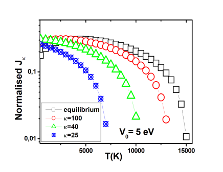
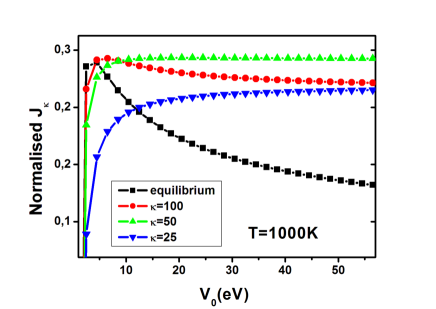
Figure 1: (color on line) Left-(A): The Normalised current density $J_{\kappa}$ with a step potential as a function of temperaure for different $\kappa$ values. Right-(B): The Normalised current density $J_{\kappa}$ with a step potential as a function of $V_{0}$ for different $\kappa$ values.

IV Barrier

The physical picture of the barrier potential would correspond to a charged current which experiences an abrupt change in potential in a given width between two regions which have the same potential. We put the barrier of thickness $d$ at $x=0$, and we label ”$1$” the negative region, ”$2$” is the label for the positive one in which the potential changes, and ”$3$” is the positive region which has the same potential as in region $1$. Namely,

$$V_{1}(x\ <\ 0)=\ 0\ \ ;\ V_{2}(0\leq x\ \leq\ d)=\ V_{0}\ \ ;\ V_{3}(x\ >\ d)=\ 0$$

As it is well known, the particles can penetrate the barrier with the minimum energy of $E_{0}=0$. Thus, we will insert this minimum value within Eq.(9) and into the corresponding norm $N$, Eq. (10). Following the general procedure, Gasiorovitz , the corresponding barrier coefficient can be found: The particles have a wavefunction $\Psi_{1}\sim exp(\pm ip_{1}x/\hbar)$ in the region $1$, and the same wavefunction in the region $3$, with momentum $p_{1}=\sqrt{2mE}$. In region $2$, corresponding to a barrier of heigth $V_{0}$, we need to distinguish between particle energies below or above $V_{0}$: If $E<V_{0}$ the wave function is written in terms of $\Psi_{2}\sim exp(\pm p_{2}x/\hbar)$, with $p_{2}=\sqrt{2m(V_{0}-E)}$. If $E>V_{0}$ the wave function becomes complex, and it is written in terms of $\Psi_{2}\sim exp(\pm ip^{\prime}_{2}x/\hbar)$ with $p^{\prime}_{2}=\sqrt{2m(E-V_{0})}$. After calculations, in the same way as in the previous section, the corresponding transmission coefficients are attained:

$$B(E<V_{0})=\left[1\ +\ \frac{\mathrm{Sinh}^{2}(p_{2}d/\hbar)}{4\dfrac{E}{V_{0}}\left[1-\dfrac{E}{V_{0}}\right]}\right]^{-1}$$ (16)

The above expression can be simplified if we dististinguish the energy ranges: If $E<<<V_{0}$, keeping the first order, Eq.(16) becomes,

$$B_{1}(E<<<V_{0})=\ 16\ \frac{E}{V_{0}}\ \mathrm{exp}\left[-\frac{2\ d}{\hbar}\sqrt{2mV_{0}}\ \right]$$ (17)

If $E\simeq V_{0}$, Eq.( 16 ) can be put as,

$$B_{2}(E\simeq V_{0})=\ \frac{1}{1+\dfrac{m\ V_{0}\ d^{2}}{2\hbar^{2}}}$$ (18)

The calculation of the transmission coefficient in the energy range $E>V_{0}$ yields,

$$B_{3}(E>V_{0})=\left[1\ +\ \frac{\mathrm{Sin}^{2}(p^{\prime}_{2}d/\hbar)}{4\dfrac{E}{V_{0}}\left[\dfrac{E}{V_{0}}-1\right]}\right]^{-1}$$ (19)

This later expression for energies $E>>>V_{0}$ can be approximated to unity.

As we have the expressions of $B(E)$, we will attain the corresponding normalised current density as

$$J_{\kappa}=\frac{1}{N}\int^{V_{0}-\Delta}_{0}\biggl{(}1\ +\frac{E-\epsilon_{F}}{E_{\kappa}+\epsilon_{F}\,}\biggr{)}^{-\kappa}\ B_{1}(E)\ dE+$$

$$+\frac{1}{N}\int^{V_{0}+\Delta}_{V_{0}-\Delta}\biggl{(}1\ +\frac{E-\epsilon_{F}}{E_{\kappa}+\epsilon_{F}\,}\biggr{)}^{-\kappa}\ B_{2}(E)\ dE+$$

$$+\frac{1}{N}\int^{+\infty}_{V_{0}+\Delta}\biggl{(}1\ +\frac{E-\epsilon_{F}}{E_{\kappa}+\epsilon_{F}\,}\biggr{)}^{-\kappa}\ B_{3}(E)\ dE$$

Where $\Delta=\alpha V_{0}$ with $0<\alpha<1$. Using Eqs. (10), (17), (18), and (19) within (IV), and after integration we obtain,

$$J_{\kappa}=\frac{\kappa-1}{\kappa-3/2}\biggl{[}\ \frac{16}{V_{0}}\ \biggl{(}\ \bm{I_{1}}(E=V_{0}-\Delta)-\bm{I_{1}}(E=0)\ \biggr{)}\ \mathrm{exp}\left\{-\frac{2\ d}{\hbar}\sqrt{2mV_{0}}\ \right\}+$$

$$+\ \left(\frac{1}{1+\dfrac{m\ V_{0}\ d^{2}}{2\hbar^{2}}}-1\right)\ \bm{I_{2}}(E=V_{0}+\Delta)\ -\ \frac{1}{1+\dfrac{m\ V_{0}\ d^{2}}{2\hbar^{2}}}\ \bm{I_{2}}(E=V_{0}-\Delta)\biggr{]}$$ (21)

where, to shorten the expression we introduce,

$$\bm{I_{1}}(E)=-\frac{E_{\kappa}^{2}\ -\kappa\ E_{\kappa}\ E+(\kappa-1)E^{2}}{(\kappa-1)(\kappa-2)\ k_{B}\ T}\biggl{(}1\ +\frac{E}{E_{\kappa}}\biggr{)}^{-\kappa}$$

$$\bm{I_{2}}(E)=-\frac{E_{\kappa}}{\kappa-1}\biggl{(}1\ +\frac{E}{E_{\kappa}}\biggr{)}^{-\kappa+1}$$

In the equilibrium limit, $\kappa\rightarrow\infty$, Eq.(IV) yields,

$$J_{\kappa\rightarrow\infty}=16\ \mathrm{exp}\left[-\frac{2\ d}{\hbar}\sqrt{2mV_{0}}\ \right]\biggl{[}\frac{k_{B}T}{V_{0}}-\ \mathrm{exp}\left(-\frac{V_{0}-\Delta}{k_{B}T}\right)\left(\frac{k_{B}T}{V_{0}}+\frac{\Delta}{V_{0}}-1\right)\biggr{]}+$$

$$+\ \frac{1}{1+\dfrac{m\ V_{0}\ d^{2}}{2\hbar^{2}}}\biggl{[}\mathrm{exp}\left(-\frac{V_{0}+\Delta}{k_{B}T}\right)-\mathrm{exp}\left(-\frac{V_{0}-\Delta}{k_{B}T}\right)\biggr{]}-\mathrm{exp}\left(-\frac{V_{0}-\Delta}{k_{B}T}\right)\ \ \$$ (22)

In this case, from Eq. (IV), we see that the transmitted current is sensitive to the mass of the incoming particles. From the above calculation we can perform an analysis of the behaviour of the current density as a function of the temperature. In this case we can realise a weak dependence on the Kappa index. Hence, the current can be considered the same for all finite Kappa values. The equilibrium $\kappa\rightarrow\infty$ can only be distinguished from the others at higher temperatures. The behaviour of the $J_{\kappa}$ as a function of $V_{0}$ is the same in the case of the current in equilibrium as for currents with finite Kappa values -all of them almost decay with the same exponential. Concerning the variation of $J_{\kappa}$ as a function of the barrier width, for an electron current the dominant term is the exponential decay with a weak dependence on the Kapppa values. The behaviour for a proton current can be seen in Figure 2. Here the Kappa value becomes significant. The value of the current density which can be transmitted will be determined by the Kappa index.

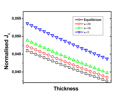
Figure 2: (color on line) Values of the transmited proton current density as a function of the thickness $d\in\left[10^{-10},10^{-4}\right]$m for a potential barrier of heigth $V_{0}=150$ $eV$. $T=5000K$.

V Hill Potential

The physical picture of the hill potential would correspond to a charged current which feels an abrupt changes at the interfaces of three regions with different potentials. The incoming current travels along a region with a ground potential. Subsequently, it penetrates into a region of width, $d$, and potential $V_{0}$. Finally the current enters into a region with a potential $V_{1}<V_{0}$, and greater than the ground. This kind of potential has been studied by Fowler concerning the thermionic emission from a metal surface. Reference Fowler takes an incoming current obeying an equilibrium Fermi-Dirac distribution. Such a later case will correspond to the equilibrium limit in this work. We set the barrier with thickness $d$ at $x=0$, and we label ”$1$” the negative region, ”$2$” is the positive one in which the potential changes to $V_{0}$, and ”$3$” is the positive region after the thickness $d$, in which the corresponding potential is $V_{1}$.

$$V_{1}(x\ <\ 0)=\ 0\ \ ;\ V_{2}(0\leq x\ \leq\ d)=\ V_{0}\ \ ;\ V_{3}(x\ >\ d)=\ V_{1}\ \ (V_{1}<V_{0})$$

In this case the particle wavefunction cannot travel across the region $3$ unless it has a minimum energy $E_{0}=V_{1}$, otherwise the corresponding wavefunction within this region would become a decreasing exponential. Therefore we insert this minimum into the corresponding norm $N$, Eq.(10) and within Eq.(9). The corresponding transmission coefficient through this kind of barrier can be found from Fowler . For convenience we perform the following changes

$$u\equiv\frac{E-V_{1}}{k_{B}T}\ ;\ \ a\equiv\frac{V_{1}-\epsilon_{F}}{k_{B}T}\ ;\ \ \gamma\equiv\frac{\epsilon_{F}}{k_{B}T}$$

Hence, we can rewrite and split Eq.(9) as follows:

$$J_{\kappa}=\frac{k_{B}T}{N}\int^{\frac{V_{0}-V_{1}}{k_{B}T}}_{0}\biggl{(}1\ +\frac{u\ +\ a}{\kappa-3/2+\gamma}\biggr{)}^{-\kappa}\ B_{1}(u)\ du+$$

$$+\frac{k_{B}T}{N}\int^{+\infty}_{\frac{V_{0}-V_{1}}{k_{B}T}}\biggl{(}1\ +\frac{u\ +\ a}{\kappa-3/2+\gamma}\biggr{)}^{-\kappa}\ B_{2}(u)\ du$$

In the evaluation of the second integral $V_{1}+uk_{B}T>V_{0}$, and therefore throughout this range of integration the transmission coefficient $B_{2}(u)$ will approximate to unity. The transmission coefficient $B_{1}(u)$ in Eq.(V), within the involved range of energies, following Fowler and using the standard procedures, can be obtained as follows,

$$B_{1}(u)=\frac{16}{V_{0}(V_{0}-V_{1})}\ \sqrt{uk_{B}T\left(V_{1}+uk_{B}T\right)}\left(V_{0}-V_{1}-uk_{B}T\right)\mathrm{exp}\left[-\frac{2\ d}{\hbar}\sqrt{2m(V_{0}-V_{1}-uk_{B}T)}\ \right]$$ (24)

The above expression with $(uk_{B}T/V_{1})<<<$ can be expanded and simplified to,

$$B_{1}(u)=\frac{16}{V_{0}}\ \sqrt{V_{1}k_{B}T}\ \ \mathrm{exp}\left[-\frac{2\ d}{\hbar}\sqrt{2m(V_{0}-V_{1})}\ \right]\ \sqrt{u}$$ (25)

If we label $U_{M}\equiv(V_{0}-V_{1})/k_{B}T$ and $Q\equiv V_{1}/k_{B}T$, and finally by inserting Eqs.(10) and (25) into Eq.(V) we attain,

$$J_{\kappa}=\biggl{(}\frac{E_{\kappa}+V_{0}}{E_{\kappa}+V_{1}}\biggr{)}^{-\kappa+1}\ \times$$

$$\times\biggl{[}1+\ \sqrt{\frac{V_{1}}{V_{0}-V_{1}}}\ \ \frac{16\ k_{B}T\left(\kappa-1\right)}{V_{0}\left(4\kappa(\kappa-2)+3\right)}\ \ C_{0}(\kappa,U_{M},Q)\ \times\ \mathrm{exp}\left[-\frac{2\ d}{\hbar}\sqrt{2m(V_{0}-V_{1})}\ \right]\biggr{]}$$

where, to shorten, the $C_{0}(\kappa,U_{M},Q)$ term reads,

$$C_{0}(\kappa,U_{M},Q)\equiv 2U_{M}-2Q+3-2\kappa(2U_{M}-1)+(2\kappa+2Q-3)\ _{2}F_{1}\left[1\ ;\frac{1}{2}-\kappa\ ;\frac{1}{2}\ ;\frac{-U_{M}}{Q+\kappa-3/2}\ \right]$$

and ${}_{2}F_{1}(a;b;c;z)$ represents the ordinary hypergeometric function, Abramovitz . By means of the corresponding calculation in the equilibrium case, we attain,

$$J_{\kappa\rightarrow\infty}=\mathrm{exp}\left(-\frac{V_{0}-V_{1}}{k_{B}T}\ \right)+\frac{16\ k_{B}T}{V_{0}}\ \sqrt{k_{B}TV_{1}}\ \ \mathrm{exp}\left[-\frac{2\ d}{\hbar}\sqrt{2m(V_{0}-V_{1})}\ \right]\ \times$$

$$\times\biggl{[}\frac{\sqrt{\pi}}{2}\ \mathrm{Erf}\left\{\sqrt{\frac{V_{0}-V_{1}}{k_{B}T}}\right\}-\ \sqrt{\frac{V_{0}-V_{1}}{k_{B}T}}\ \mathrm{exp}\left(-\frac{V_{0}-V_{1}}{k_{B}T}\ \right)\ \biggr{]}$$ (27)

where $\mathrm{Erf}(x)$ stands for the Error function, Abramovitz . In Figure 3 we observe the corresponding normalised current as a function of temperature: The transmitted currents out of equilibrium (with low $\kappa$ values) are greater than the classical Fermi-Dirac case corresponding to equilibrium. In all cases, the current is almost constant with the temperature. Figure 4 shows the normalised current as a function of the $V_{1}$ potential. For all Kappa values the current decays as the potential increases, but the value of the current density when the fermionic poulation departs from the classical Fermi-Dirac distribution becomes greater. In Figure 5 we observe the decay of currents with different Kappa values as a function of the quotient $V_{0}/V_{1}$. In this case the decay is faster for the equilibrium ($\kappa\rightarrow\infty$) currents.

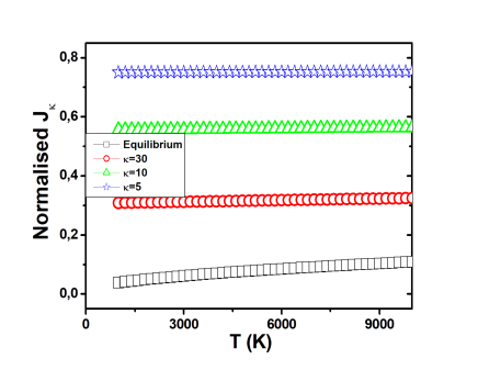
Figure 3: (color on line) Values of the transmited proton current density as a function of the temperature through a hill potential barrier of heigth $V_{1}=200$ $eV$, $V_{0}/V_{1}=1.3$.

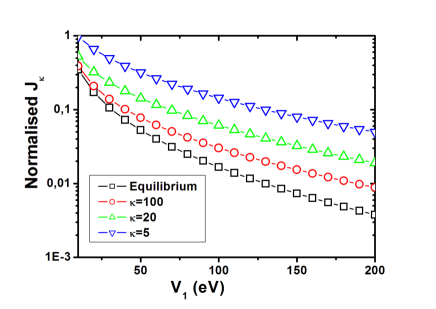
Figure 4: (color on line) Values of the transmited proton current density as a function of $V_{1}$ through a hill potential barrier at temperature $T=5000K$, with $V_{0}/V_{1}=3.5$.

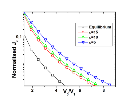
Figure 5: (color on line) Values of the transmited proton current density as a function of $V_{0}/V_{1}$ through a hill potential barrier at temperature $T=5000K$, with $V_{1}=0.5$ $eV$.

VI Conclusions.

In this work, we use the generalised Fermi Dirac distribution function to build a current. These currents have been studied travelling through several barriers with different representative shapes as: The step potential, the potential barrier, and also the hill potential. The resulting currents have been later compared with those of the equilibrium limit. The transmitted current through both the step and hill potentials are quite sensitive to the shape of the potential as well as to the degree of departure from equilibrium. On the contrary, concerning the barrier, the transmission is almost independent of the Kappa values for electron currents, and sligthy in the case of protons. A subsequent task coming up here is to study the transmission of a Kappa current through a (smoothed) barrier of an arbitrary shape. This task could be done following the same procedure we follow along this work. Previously, the corresponding transmission coefficient could be computed as a juxtaposition of square potential barriers of thickness $\Delta x$. The height of potential would be suitable to the corresponding height of the modelled potential at this $x$ point, $V(x)$. Using the WKB approximation this could be written as:

$$\mathrm{ln}\left[B(E)\right]\approx-2\ \int_{\forall Barrier}\ dx\sqrt{2m(V(x)-E)/\hbar^{2}}$$

and later inserting such a term into Eq.(9) to obtain the transmitted current. However, it entangles to fit numerically to the modelled potential the height of $V(x)$, as well as the thickness $\Delta x$. Hence, this task turns out to be a numerical issue, which is left for a further work.

References

- (1) R.D. Evans The Atomic Nucleus Kieger publishing Company, (1985).
- (2) C. Rolfs, H.P. Trautvetter and W. S.Rodney Current status of nuclear astrophysics Rep. Prog. Phys. 50, (1987) 233.
- (3) C. Kittel Introduction to Solid State Physics John Wiley and Sons, Chapter 7, (1996).
- (4) O.W. Richardson, Emission of electricity from hot bodies. Monographs on Physics. Longmans, Green and Co. (1916).
- (5) S. Dushmann, Thermionic Emission Rev. of Mod. Phys. 4(2),(1930) 381.
- (6) Fowler R.H., The Thermionic Emission Constant A Proc. Roy. Soc. A, DOI 10.1098/rspa.1929.0003, (1929).
- (7) R.A. Treumann, Quantum-Statistical Mechanics in the Lorentzian Domain, Europhys. Lett. 48 (1),(1999) 8.
- (8) R.A. Treumann, Kinetic Theoretical Foundation of Lorentzian Statistical Mechanics, Phys. Scr. 59,(1999) 19.
- (9) J.J. Podesta, Plasma Dispersion Function for the Kappa distribution, NASA Reports, CR-2004-212770, (2004).
- (10) B.D. Shizgal, Suprathermal particle distributions in space physics: Kappa distributions and entropy. Astrophys. Space Sci. 312, (2007) 227.
- (11) J.L. Domenech-Garret, Non equilibrium approach regarding metals from a linearised Kappa distribution, J. of Stat. Mech. 10,P103206 (2017) 1.
- (12) N.D. Ascroft, N.D. Mermin, Solid State Physics, Harcourt College Publishers (1976), Chapter 13.
- (13) Chang Sub Kim, B. Shizgal, Relaxation of hot-electron distributions in GaAs, Phys. Rev. B 44(7),(1991) 2969.
- (14) B. Shizgal, Kappa and other nonequilibrium distributions from the Fokker-Planck equation and the relationship to Tsallis entropy, Phys. Rev. E 97, (2018) 052144.
- (15) J.L. Domenech-Garret, S.P. Tierno and L. Conde, Enhanced thermionic currents by non equilibrium electron populations of metals, Eur. Phys. J. B 86,(2013) 382.
- (16) J.L. Domenech-Garret, Generalized electrical conductivity and the melting point of thermionic metals, J. of Stat. Mech. 8,P08001 (2015) 1.
- (17) J.L. Domenech-Garret, Non equilibrium thermal and electrical transport coefficients for hot metals, High Temperatures-High Pressures 46(4-5),(2017) 1. arXiv:1701.06598 [cond-mat.mes-hall].
- (18) J.L. Domenech-Garret, S.P. Tierno, and L. Conde Non-equilibrium thermionic electron emission for metals at high temperatures J. of Appl. Phys. 118,(2015) 074904.
- (19) S. Gasiorowitz Quantum Physics John Wiley ed, (1972).
- (20) M. Abramowitz and I. A. Stegun Handbook of Mathematical Functions National Bureau of Standards, (1972).