Label-Aware Graph Convolutional Networks

Abstract.

Recent advances in Graph Convolutional Networks (GCNs) have led to state-of-the-art performance on various graph-related tasks. However, most existing GCN models do not explicitly identify whether all the aggregated neighbors are valuable to the learning tasks, which may harm the learning performance. In this paper, we consider the problem of node classification and propose the Label-Aware Graph Convolutional Network (LAGCN) framework which can directly identify valuable neighbors to enhance the performance of existing GCN models. Our contribution is three-fold. First, we propose a label-aware edge classifier that can filter distracting neighbors and add valuable neighbors for each node to refine the original graph into a label-aware (LA) graph. Existing GCN models can directly learn from the LA graph to improve the performance without changing their model architectures. Second, we introduce the concept of positive ratio to evaluate the density of valuable neighbors in the LA graph. Theoretical analysis reveals that using the edge classifier to increase the positive ratio can improve the learning performance of existing GCN models. Third, we conduct extensive node classification experiments on benchmark datasets. The results verify that LAGCN can improve the performance of existing GCN models considerably, in terms of node classification.

1. Introduction

Node classification, which aims at classifying nodes in a graph, is one of the most common applications in graph-related literatures (bhagat2011node, ; perozzi2014deepwalk, ; grover2016node2vec, ; wang2014mmrate, ), e.g., classifying the documents in a citation network. Recently, the Graph Convolutional networks (GCNs) which extend the Convolutional Neural Networks (CNNs) to the non-Euclidean graph domain are gaining increasing research interests. They have been successfully applied to node classification and achieved the state-of-the-art performances (kipf2016gcn, ; velivckovic2017gat, ; zhang2018gaan, ; huang2018asgcn, ; chen2018fastgcn, ; zeng2019graphsaint, ; rong2019dropedge, ). These successes also encourage the burst of many variants, including GraphSAGE (hamilton2017graphsage, ), simplified GCN (SGC) (wu2019sgc, ), ASGCN (huang2018asgcn, ), FastGCN (chen2018fastgcn, ), and GAT (velivckovic2017gat, ), etc.

Generally, in most GCN models, the state of each node is iteratively updated by its own state and the states aggregated from its neighbors (li2018laplacian, ; wu2019sgc, ). The final output (e.g., the predicted label of the node class) is produced based on the aggregated node states. As such, the performance of GCN models is largely effected by the quality of the aggregated neighbors. However, existing GCN models do not explicitly identify whether the aggregated neighbors are valuable to the node classification or investigate how to enhance the accuracy of GCN models by refining the graph structure. In this case, the classification result may be misled by the information aggregated from distracting neighbors.

A number of recent works generalize the graph convolution with the attention mechanism (velivckovic2017gat, ; zhang2018gaan, ). For example, GAT (velivckovic2017gat, ) dynamically assigns an aggregation weight to each neighbor, which, to some extent, can control the aggregation from distracting neighbors. However, the attention layers are not trained with an explicit criterion to identify whether one neighbor is informative or distracting; besides, the attention layers cannot help one node to gain information from other non-connected but valuable nodes. Consequently, the attention mechanism may have little effect when the target node has very few informative neighbors. In addition, it is also hard for other GCN models with different architectures to reuse the trained attention weights directly.

In this paper, we propose the Label-Aware GCN (LAGCN) framework which can refine the graph structure before the training of GCN, such that existing GCN models can directly benefit from LAGCN without changing their model architectures. The main contribution is three-fold.

• We point out and verify that in node classification tasks, the same-label neighbors are valuable (positive) neighbors while the different-label neighbors are distracting (negative) neighbors. Then we propose an edge classifier to refine the original graph structure into a label-aware (LA) graph structure by 1) filtering the negative neighbors and 2) adding more non-connected but positive nodes as new neighbors. Existing GCN models can be trained directly over the LA graph to improve their performance, without changing their model architectures.

• We introduce the concept of positive ratio to evaluate the density of valuable neighbors in the LA graph and prove that the performance of GCN is positively correlated to the positive ratio from a theoretical standpoint. On this basis, we give the minimum requirements of building an effective edge classifier and reveal how the edge classifier influences the classification performance.

• We conduct extensive experiments on benchmark datasets and verify that the LAGCN can improve the node classification performances of existing GCN models (including GAT) considerably, especially when the underlying graph has a low positive ratio.

2. Preliminaries

In this paper, we consider the node classification problem on a directed graph $\textbf{G}=(\textbf{V},\textbf{E})$ with $N$ nodes and $E$ edges. The edge between node $u,v\in\textbf{V}$ is denoted as $(u,v)\in\textbf{E}$. The binary adjacency matrix with self-loop edges is denoted as $\textbf{A}\in\mathbb{R}^{N\times N}$. Let $\textbf{X}=\{\textbf{x}_{1},\textbf{x}_{2},\cdots,\textbf{x}_{N}\}$ denote the feature of the nodes and $Y=\{y_{1},y_{2},\cdots,y_{N}\}$ denote the labels of all the nodes. Let $C$ denotes the total class number, $\mathcal{N}_{v}$ denotes the set of all $1$-hop neighbors of node $v$ and $n_{v}=|\mathcal{N}_{v}|$ denotes the number of $1$-hop neighbors of node $v$. The hidden embedding of node $v$ on the $k$-th GCN layer is denoted as $\textbf{h}_{v}^{(k)}$. The initial node embedding at the first layer is generated with the raw feature X.

Generally, most existing GCNs are constructed by stacking multiple first-order graph convolution layers. Specifically, the embedding of node $v$ at the $(l+1)$-th layer of an GCN can be computed as

(1) $$\textbf{h}_{v}^{(l+1)}=\sigma\Big{(}\textbf{FC}_{\theta_{(l)}}\big{(}\sum\nolimits_{u\in{\mathcal{N}_{v}}}w^{(l)}_{u,v}\textbf{h}^{(l)}_{u}\big{)}\Big{)},$$

where $\textbf{FC}_{\theta_{(l)}}$ refers to a fully-connect layer with the parameter $\theta_{(l)}$; $w^{(l)}_{v,u}$ denotes the aggregation weight of the neighboring nodes $u\in{\mathcal{N}_{v}}$; $\sigma$ denotes the non-linear activation function. In GAT (velivckovic2017gat, ), the aggregation weights (i.e., attention weights) are determined based on a multi-head attention mechanism. While in sampling-based GCNs (hamilton2017graphsage, ; chen2018fastgcn, ; huang2018asgcn, ), the central node $v$ samples a subset of the neighbors $\mathcal{N}_{v}^{\prime}$ for aggregation based on certain pooling methods, e.g., mean pooling.

Noticeably, the recently proposed Simplified Graph Convolutional Networks (SGC) (wu2019sgc, ) reveals that the nonlinearity between consecutive convoulutional layers can be unnecessary. Hence, SGC removes the non-linear activation functions such that the node embedding at the $(l+1)$-th layer of SGC can be simplified as

(2) $$\textbf{h}_{v}^{(l+1)}=\frac{1}{n_{v}}\sum\nolimits_{u\in{\mathcal{N}_{v}}}\textbf{h}^{(l)}_{u}.$$

After computing the hidden embedding of $K$-th layer, SGC predicts the labels of nodes with a single linear layer and achieves comparable performance as GCN.

3. Lable-Aware GCN Framework

In this section, we introduce the concept of positive ratio, discuss how to build an effective edge classifier, and analyze the correlation between the positive ratio and classification performance from a theoretical standpoint.

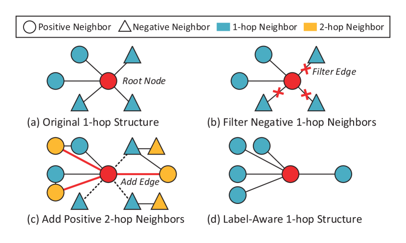
Figure 1. Illustration of the graph refinement process.

Given a target node, its neighbors can be classified into two types, i.e., the positive ones and the negative ones.

Definition 3.1.

Given a target node $v$, its positive (or negative) neighbor set $\mathcal{N}^{+}_{v}$ (or $\mathcal{N}^{-}_{v}$) is the set of neighbors whose labels $y_{u}$ are the same as (or different from) $y_{v}$.

As such, the update function of node $v$ in (1) can be rewritten as

(3) $$\textbf{h}_{v}^{(l+1)}=\sigma\Big{(}\textbf{FC}_{\theta_{(l)}}(\sum\nolimits_{u\in{\mathcal{N}^{+}_{v}}}w^{(l)}_{v,u}\textbf{h}_{u}^{(l)}+\sum\nolimits_{u\in{\mathcal{N}^{-}_{v}}}w^{(l)}_{v,u}\textbf{h}_{u}^{(l)})\Big{)}.$$

According to SGC (wu2019sgc, ), the nonlinearity between GCN layers can be unnecessary since the main benefits come from the local averaging. Therefore, we here develop our theoretical analysis without considering the nonlinear functions (including the fully-connected layer and the activation function) in GCNs for analytical purposes. In this case, the update function of node $v$ can be written as

(4) $$\textbf{h}_{v}^{(l)}=\frac{1}{n_{v}}(\sum\nolimits_{u\in{\mathcal{N}^{+}_{v}}}\textbf{h}_{u}^{(l-1)}+\sum\nolimits_{u\in{\mathcal{N}^{-}_{v}}}\textbf{h}_{u}^{(l-1)}).$$

With the simplified graph convolution, the embedding of different layers locates at the same hidden space. Next, we demonstrate that the probability of generating a correct classification result is correlated to the positive ratio. Without loss of generality, we consider a binary classification problem with the following assumptions.

• Given a linear function $F$ which projects the hidden embedding $\textbf{h}_{u}^{(l-1)}$ to a real number prediction of node $u$, such as the linear function of SGC. We classify one node $u$ into the positive class if $F(\textbf{h}_{u}^{(l-1)})>\tau$, or negative class otherwise, where $\tau$ denotes the classification threshold.

• We assume that the prediction of $F(\cdot)$ obeys a Gaussian mixture distribution, i.e., $F(\textbf{h}_{u}^{(l-1)}){iid\atop\sim}Norm(\mu^{+},\sigma^{2})$ for $u\in\mathcal{N}^{+}_{i}$ and $F(\textbf{h}_{u}^{(l-1)}){iid\atop\sim}Norm(\mu^{-},\sigma^{2})$ for $u\in\mathcal{N}^{-}_{i}$. Empirically, we consider $\mu^{+}$ to be larger than $\tau$, and $\mu^{-}$ otherwise.

In this way, $F(\textbf{h}_{v}^{(l)})$ can be written as

(5) $$F(\textbf{h}_{v}^{(l)})=\frac{1}{n_{v}}\Big{(}\sum\nolimits_{u\in{\mathcal{N}_{v}^{+}}}F(\textbf{h}_{u}^{(l-1)})+\sum\nolimits_{u\in{\mathcal{N}_{v}^{-}}}F(\textbf{h}_{u}^{(l-1)})\Big{)}.$$

Then the expectation of $F(\textbf{h}_{v}^{(l)})$ can be written as

(6) $$E_{origin}=E(F(\textbf{h}_{v}^{(l)}))=\dfrac{1}{n_{v}}(n^{+}_{v}\mu^{+}+n^{-}_{v}\mu^{-})=r_{v}\mu^{+}+(1-r_{v})\mu^{-},$$

where $r_{v}=n_{v}^{+}/(n_{v}^{+}+n_{v}^{-})=n_{v}^{+}/n_{v}$ denotes the positive ratio of node $v$. Therefore, we can enhance the probability of correctly classifying node $v$ by increasing its positive ratio $r_{v}$. Similarly, we can enhance the probability of correctly classifying each node in a graph by increasing the positive ratio of the entire graph, which leads to the following proposition.

Proposition 1.

The probability of correctly classifying the nodes $v\in\textbf{V}$ in a graph can be increased by improving the positive ratio of the entire graph $R=\sum_{v\in\textbf{V}}n_{v}^{+}/(\sum_{v\in\textbf{V}}n_{v})$.

Label-Aware Graph Refinement. We now build an edge classifier to identify positive and negative neighbors for each node in a graph. In particular, we refer to the edges between the node with the positive neighbors (or negative neighbors) as a positive edge (or negative edge). Given an edge $(u,v)$, the aim of the edge classifier $\mathcal{E}$ is to return a binary value $\hat{y}_{u,v}$ which specifies whether the edge $(u,v)$ is a positive edge, i.e., $\hat{y}_{u,v}=1$ or a negative edge, i.e., $\hat{y}_{u,v}=0$. The edge classifier $\mathcal{E}$ can be readily trained using the binary adjacency matrix A, the node feature matrix X, and the labels of the train set $Y_{train}$ in the original graph.

In this paper, we build the edge classifier with multi-layer perception (MLP) layers. Specifically, given the features of two nodes as $\textbf{e}_{u}$ and $\textbf{e}_{v}$, the binary value of their edge is computed as

(7) $$\mathcal{E}(u,v)=\textbf{MLP}\left\{|\hat{\textbf{e}}_{u}-\hat{\textbf{e}}_{v}|\ \oplus\ (\hat{\textbf{e}}_{u}+\hat{\textbf{e}}_{v})\ \oplus\ (\hat{\textbf{e}}_{u}\circ\hat{\textbf{e}}_{v})\right\},$$

where $\oplus$ denotes the concatenation operation, MLP denotes the function of multi-layer perception, and $\hat{\textbf{e}}_{u}=\textbf{e}_{u}\textbf{W}_{e}$ denotes the low-dimensional feature projected from $\textbf{e}_{u}$ to accelerate the prediction process with $\textbf{W}_{e}$ the projecting weights. Note that using MLP layers to build an edge classifier is only one possible solution, other designs could be explored in the future.

The original graph structure can then be refined into a label-aware graph structure to increase the positive ratio $R$ based on the edge classifier. Specifically, the graph refinement process contains the following two steps. 1) Filtering process: as shown in Figure 1(b), for each node in a graph, we use the trained edge classifier to predict whether its 1-hop neighbors are positive neighbors, then we delete all of its negative neighbors. 2) Adding process: as shown in Figure 1(c), for each node, we use the trained edge classifier to predict whether its 2-hop neighbors are positive neighbors, then we add edges between this node and its positive 2-hop neighbors, turning them into positive 1-hop neighbors, until the total number of 1-hop neighbors reaches a preset number $n_{max}$.

Theoretical Analysis. We now analyze why learning from the LA-graph leads to superior learning performance and give the minimum requirements for building an effective edge classifier.

In the filtering process, we delete all the predicted negative edges ($\hat{y}_{u,v}=0$) between the central node $v$ and its 1-hop neighbors. The filtering process preserves two types of neighbors: 1) the positive neighbors which are predicted to be positive, i.e., $y_{u,v}=1$ and $\hat{y}_{u,v}=1$; 2) the negative neighbors which are predicted to be positive, i.e., $y_{u,v}=0$ and $\hat{y}_{u,v}=1$. Suppose that before the filtering process, the number of positive (or negative) neighbors for node $v$ is $n_{v}^{+}$ (or $n_{v}^{-}$). Then, after filtering the predicted-negative edges, the number of positive (or negative) neighbors for node $v$ turns to be $p\cdot n_{v}^{+}$ (or $q\cdot n_{v}^{-}$) where $p={\rm P}(\hat{y}_{u,v}=1|y_{u,v}=1)$ and $q={\rm P}(\hat{y}_{u,v}=1|y_{u,v}=0)$. As such, the expectation of $F(\textbf{h}_{v}^{(l)})$ can be given as

(8) $$E_{filter}=\frac{p\cdot n^{+}_{v}\mu^{+}+q\cdot n^{-}_{v}\mu^{-}}{p\cdot n_{v}^{+}+q\cdot n_{v}^{-}}.$$

In order to ensure $E_{filter}$ to be greater than $E_{origin}$, the edge classifier should satisfy the following proposition.

Proposition 2.

Let $p={\rm P}(\hat{y}_{u,v}=1|y_{u,v}=1)$ and $q={\rm P}(\hat{y}_{u,v}=1|y_{u,v}=0)$, the filtering process can enhance the performance of the GCN models as long as $p>q$.

In the adding process, we iteratively add edges between the central node $v$ and its predicted-positive 2-hop neighbors ($\hat{y}_{u,v}=1$), i.e., turning them into 1-hop neighbors, until the total number of 1-hop neighbors reaches a preset number. Suppose that before the adding process, the number of positive (or negative) neighbors of node $v$ is $n_{v}^{+}$ (or $n_{v}^{-}$) and the number of added 1-hop neighbors is $n_{v}^{\prime}$. After the adding process, the number of its positive and negative neighbors turns to be $n_{v}^{+}+p_{pre}\cdot n_{v}^{\prime}$ and $n_{v}^{-}+(1-p_{pre})\cdot n_{v}^{\prime}$, respectively, where $p_{pre}={\rm P}(y_{u,v}=1|\hat{y}_{u,v}=1)$ and $1-p_{pre}={\rm P}(y_{u,v}=0|\hat{y}_{u,v}=1)$. The expectation of the prediction $F(\textbf{h}_{v}^{(l)})$ can be written as

(9) $$E_{add}=\frac{(n^{+}_{v}+p_{pre}\cdot n_{v}^{\prime})\mu^{+}+(n^{-}_{v}+(1-p_{pre})\cdot n_{v}^{\prime})\mu^{-}}{n_{v}^{+}+n_{v}^{-}+n_{v}^{\prime}}.$$

In order to ensure $E_{add}$ to be greater than $E_{origin}$, an effective edge classifier should satisfy the following proposition.

Proposition 3.

Let $p_{pre}={\rm P}(y_{u,v}=1|\hat{y}_{u,v}=1)$, the adding process can enhance the performance of GCN as long as $p_{pre}>r_{v}$.

4. EXPERIMENT

Datasets. We use four benchmark datasets, i.e., Cora, Citeseer, Pubmed and Reddit (hamilton2017graphsage, ), where the number of nodes scales as $O(10^{3})$, $O(10^{3})$, $O(10^{4})$, and $O(10^{5})$, respectively.
Settings. The edge classifier is trained with the nodes and edges in the training set. For Pubmed, we use the raw feature as the input features for edge classifier. For Cora, Citeseer, and Reddit, we use $\textbf{A}^{2}\textbf{X}$ (wu2019sgc, ) as the input features for edge classifier. For the adding process, we set the maximum number of 1-hop neighbors as $6$ for both Cora and Citeseer, and as $30$ for Pubmed and Reddit. The maximum numbers are selected to be $20\%$ larger than the sampling number of GraphSAGE (hamilton2017graphsage, ). Code will be released later to ensure reproducibility.
Baseline models. We select GCN (kipf2016gcn, ), GAT (velivckovic2017gat, ), and SGC (wu2019sgc, ) GraphSAGE (hamilton2017graphsage, ) and ASGCN (huang2018asgcn, ) as the baseline models. For Cora, Citeseer and Pubmed, GCN, GAT, and SGC are trained with semi-supervised setting, i.e., only use a small part of nodes in the training set to optimize their parameters, while GraphSAGE and ASGCN are trained with full-supervised setting. For Reddit, SGC, GraphSAGE, and ASGCN are trained with full-supervised setting.

Table 1. Accuracy of the LA-GCNs against the origin-GCNs

	Cora	Citeseer	Pubmed	Reddit
ori-R/LA-R	85%/90%	74%/82%	80%/96%	78%/95%
origin-GCN	0.8180	0.7090	0.7850	-
LA-GCN	0.8330	0.7330	0.8780	-
origin-GAT	0.8300	0.7250	0.7900	-
LA-GAT	0.8350	0.7360	0.8690	-
origin-SGC	0.8210	0.7190	0.7890	0.9488
LA-SGC	0.8380	0.7340	0.8770	0.9540
origin-SAGE	0.8650	0.7850	0.8830	0.9540
LA-SAGE	0.8840	0.8000	0.9070	0.9673
origin-ASGCN	0.8740	0.7960	0.9060	0.9627
LA-ASGCN	0.8880	0.8010	0.9170	0.9758

Table 2. Performance under low positive ratio.

	Cora	Citeseer	Pubmed
ori-R(low)/LA-R(low)	30%/67%	24%/74%	34%/95%
origin-GCN(low)	0.3920	0.3820	0.5810
LA-GCN(low)	0.6690	0.6650	0.8780
origin-GAT(low)	0.4430	0.3580	0.6020
LA-GAT(low)	0.6850	0.6750	0.8850

Main Results. Table 1 shows the node classification performance of all comparing methods on different datasets. Specifically, the first row of Table 1 presents the positive rate of original graphs and LA-graphs, while the other rows present the performance of the baseline GCN models and their LA enhanced versions. The results verify that our proposed LAGCN framework can improve the node classification performance of existing GCN models considerably. In other words, increasing the positive ratio of the underlying graph can lead to better classification performance for GCN models, i.e., Theorem 1. Moreover, the results also show that 1) the original GAT outperforms the original GCN and the original SGC; however, both the LA-SGC and the LA-GCN perform better than the original GAT, which indicates that the LAGCN framework is more effective than the attention mechanism; 2) the LA-GAT outperforms the original GAT, which indicates that LAGCN can complement the attention mechanism to reach a better performance.

Influence from the adding and filtering process. In Figure 2, we evaluate the influence of the adding and filtering process, respectively. The filter-graph only filters the negative edges; the add-graph only adds more positive edges; the LA-graph both filters the negative edges and adds more positive edges. This figure demonstrates that both the filtering and the adding process can enhance the performance of the GCN models. Meanwhile, they can complement each other to reach the best performance. Note that similar conclusions can also be drawn from the other datasets, we omit the results here due to space limit.

Influence from the edge classifier. In Figure 3, we study the influence of the edge classifier by artificially modifying the $p-q$ and $p_{pre}$ with the ground truth testing labels and evaluating it with LA-SGC. The sub-figure on the left panel shows that the performance of the LA-models is positively correlated to the value of $p-q$, which verifies Theorem 2. The sub-graph on the right panel shows that the performance of LA-models is positively correlated to the value of $p_{pre}$, which verifies Theorem 3.

Performance under low positive ratio. We add 5 different-label neighbors to each node in Cora, Citeseer and 15 different-label neighbors in Pubmed so as to artificially decrease their positive ratio from $85\%$, $74\%$, $80\%$ to $30\%$, $24\%$, $34\%$, respectively, and test the performance of GCN and GAT. The LA classifier used in LA-GCN and LA-GAT are trained with the raw features and can improve the positive ratio back to $67\%$, $74\%$, $95\%$, respectively. The results in Table 2 show that LA-GCN and LA-GAT are much more robust than GCN and GAT when the graph has a lower positive ratio.

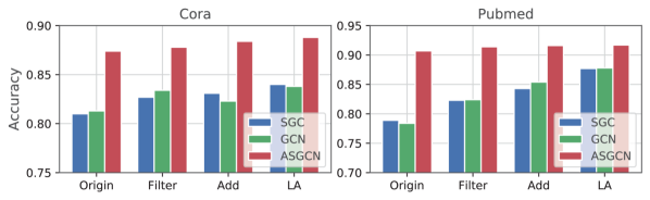
Figure 2. Influence from the adding and filtering process.

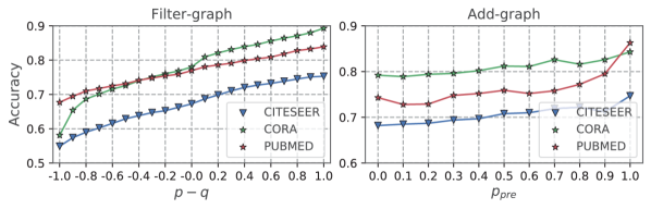
Figure 3. Influence from the edge classifier.

5. Conclusion

In this paper, we propose the LAGCN framework, which can increase the positive ratio of the learning graph by training an edge classifier to filter the negative neighbors and add new positive neighbors for each node in the graph. Experimental results verify that existing GCN models can directly benefit from LAGCN to improve their node classification performances.

6. Acknowledgement

This work is supported in part by the National Natural Science Foundation of China (Grand Nos. U1636211, 61672081, 61370126) and 2020 Tencent Wechat Rhino-Bird Focused Research Program and China Postdoctoral Science Foundation (No. 2020M670337).

References

- [1] Smriti Bhagat, Graham Cormode, and S Muthukrishnan. Node classification in social networks. In Social network data analytics, pages 115–148. Springer, 2011.
- [2] Jie Chen, Tengfei Ma, and Cao Xiao. FastGCN: fast learning with graph convolutional networks via importance sampling. ICLR, 2018.
- [3] Aditya Grover and Jure Leskovec. node2vec: Scalable feature learning for networks. In SIGKDD, pages 855–864. ACM, 2016.
- [4] Will Hamilton, Zhitao Ying, and Jure Leskovec. Inductive representation learning on large graphs. In NIPS, 2017.
- [5] Wenbing Huang, Tong Zhang, Yu Rong, and Junzhou Huang. Adaptive sampling towards fast graph representation learning. In NIPS, 2018.
- [6] Thomas N Kipf and Max Welling. Semi-supervised classification with graph convolutional networks. arXiv preprint arXiv:1609.02907, 2016.
- [7] Qimai Li, Zhichao Han, and Xiao-Ming Wu. Deeper insights into graph convolutional networks for semi-supervised learning. In AAAI, 2018.
- [8] Bryan Perozzi, Rami Al-Rfou, and Steven Skiena. Deepwalk: Online learning of social representations. In SIGKDD, pages 701–710. ACM, 2014.
- [9] Yu Rong, Wenbing Huang, Tingyang Xu, and Junzhou Huang. Dropedge: Towards the very deep graph convolutional networks for node classification. ICLR, 2020.
- [10] Petar Veličković, Guillem Cucurull, Arantxa Casanova, Adriana Romero, Pietro Lio, and Yoshua Bengio. Graph attention networks. ICLR, 2019.
- [11] Senzhang Wang, Xia Hu, Philip S Yu, and Zhoujun Li. Mmrate: inferring multi-aspect diffusion networks with multi-pattern cascades. In KDD, 2014.
- [12] Felix Wu, Tianyi Zhang, Amauri Holanda de Souza Jr, Christopher Fifty, Tao Yu, and Kilian Q Weinberger. Simplifying graph convolutional networks. ICML, 2019.
- [13] Hanqing Zeng, Hongkuan Zhou, Ajitesh Srivastava, Rajgopal Kannan, and Viktor Prasanna. Graphsaint: Graph sampling based inductive learning method. ICLR, 2020.
- [14] Jiani Zhang, Xingjian Shi, Junyuan Xie, Hao Ma, Irwin King, and Dit-Yan Yeung. Gaan: Gated attention networks for learning on large and spatiotemporal graphs. WWW, 2018.