Efficient simulation of filament elastohydrodynamics in three dimensions

Abstract

Fluid-structure simulations of slender inextensible filaments in a viscous fluid are often plagued by numerical stiffness. Recent coarse-graining studies have reduced the computational requirements of simulating such systems, though have thus far been limited to the motion of planar filaments. In this work we extend such frameworks to filament motion in three dimensions, identifying and circumventing coordinate-system singularities introduced by filament parameterisation via repeated changes of basis. The resulting methodology enables efficient and rapid study of the motion of flexible filaments in three dimensions, and is readily extensible to a wide range of problems, including filament motion in confined geometries, large-scale active matter simulations, and the motility of mammalian spermatozoa.

I Introduction

The coupled elasticity and hydrodynamics of flexible inextensible filaments on the microscale are of significance to much of biology, biophysics and soft matter physics. For example, many organisms possess slender flagella or cilia, utilised for driving flows and even locomotion, whilst investigation into the role of synthetic filaments as both soft deformable sensors and methods of propulsion has been the subject of recent enquiry [1, 2, 3, 4, 5, 6, 7, 8, 9]. As a result, the complex mechanics of fluid-structure interaction has been well-studied, utilising methods such as the slender body and resistive force theories of Hancock [2], Gray and Hancock [10], Johnson [11], through to the exact representations of boundary integral methods as used by Pozrikidis [12, 6, 7]. A fundamental barrier to much numerical investigation has been the severe stiffness associated with the equations of filament elasticity when coupled to viscous fluid dynamics. Hence, as remarked in the recent and extensive review of du Roure et al. [13], an appropriate framework, capable of realising efficient simulation of filament elastohydrodynamics, is crucial for the numerical study of filament mechanics.

Recently, significant progress has been made in resolving the dynamics of planar filaments, with the work of Moreau et al. [14] presenting a coarse-grained model of filament elasticity that overcame much of the stiffness previously associated with slender elastohydrodynamics. Key to this approach was the integration of the pointwise force and moment balance equations, the spatial discretisation of which yielded a relatively simple system of ordinary differential equations to solve in order to describe filament motion. Additionally demonstrated to be flexible in the original publication of Moreau et al., this framework has been extended to include non-local hydrodynamics in both infinite and semi-infinite domains, and applied to a variety of single and multi-filament problems [15, 16]. However, being confined to two dimensions limits the potential scope and applicability of these approaches, with three dimensional filament motion being readily and frequently observed in a plethora of biophysical systems, such as the complex flagellar beating found in spermatozoa or the helically-driven monotrichous bacterium Escherichia coli [17, 3].

However, for non-planar filaments in three dimensions there is currently no methodology analogous to that of Moreau et al., with state-of-the-art frameworks still plagued by extensive numerical stiffness, necessitating costly computation to the extent that practical simulation studies have been limited and parameter space studies are largely prohibited. With three dimensions inherently more challenging than lower dimensional settings, this field has seen developments such as the recent work of Schoeller et al. [18], which utilises a quarternion representation of filament orientation to parameterise the three dimensional shape of the slender body. However, in this framework, numerical care is required to satisfy the inextensibility condition, with similar such consideration necessary in the earlier methodologies of Olson et al. [19], Simons et al. [20], Ishimoto and Gaffney [21], Bouzarth et al. [22], each of which are equipped with non-local slender-body hydrodynamics and consider nearly inextensible filaments. Consequently, these existing approaches often require the use of sophisticated computing hardware in order to simulate filament motion, with typical simulations of Ishimoto and Gaffney having a runtime of multiple hours on high performance computing clusters. The recent work of Jabbarzadeh and Fu [23] compared and contrasted these nearly inextensible approaches with a truly inextensible scheme, concluding that both accuracy and efficiency was afforded by the latter in a range of biological and biophysical modelling scenarios. Despite their improved efficiency, typical walltimes for these filament simulations are measured on a timescale of hours on typical hardware. Thus, there remains significant scope for the development of an efficient framework for the simulation of inextensible elastic filaments in three dimensions, one in which filament dynamics can be rapidly computed on non-specialised hardware on timescales of seconds or minutes, thus facilitating a wealth of future studies and explorations into complex and previously intractable biological and physical systems.

Hence, the fundamental objective of this study is to develop and describe an efficient framework for the numerical simulation of filament mechanics in three dimensions. We will build upon the recent and significant work of Moreau et al. [14], extending their approach to include an additional spatial dimension via a generalisation of the Frenet triad and integration of the governing equations of elasticity. We will overcome fundamental issues with simple single parameterisations of a filament in three dimensions, presenting an effective computational approach utilising adaptive reparameterisation and basis selection. We will then validate the presented framework by consideration of three candidate test problems, simulating well-documented behaviours of filaments in a viscous fluid and including a side-by-side comparison against the existing and recent methodology of Ishimoto and Gaffney [21]. Finally, we will showcase the flexibility and general applicability of the presented approach by describing and exemplifying a number of methodological extensions.

II Methods

II.1 Equations of elasticity

We consider a slender, inextensible, unshearable filament in a viscous Newtonian fluid, with its centreline described by $\bm{x}(s)$, parameterised by arclength $s\in[0,L]$ for dimensional filament length $L$. We model the filament as a Kirchhoff rod with arclength-independent material parameters, circular cross-sections, and, in the first instance, no intrinsic curvature or intrinsic torsion. Both the filament and fluid inertia are negligible for the physical scales associated with many applications, especially those associated with cellular flagella and cilia; hence there is no inertia here and throughout. Along the filament we have the pointwise conditions of force and moment balance, given explicitly by

$$\bm{n}_{s}-\bm{f} =\bm{0}\,,$$ (1)

$$\bm{m}_{s}+\bm{x}_{s}\times\bm{n}-\bm{\tau} =\bm{0}\,,$$ (2)

for contact force and torque denoted $\bm{n},\bm{m}$ respectively and where a subscript of $s$ denotes differentiation with respect to arclength. The quantity $\bm{f}$ is the force per unit length applied on the fluid medium by the filament, which we will later express in terms of the filament velocity $\dot{\bm{x}}$, where here a dot denotes a time derivative. Similarly, $\bm{\tau}$ is the torque per unit length applied on the fluid medium by the filament. Whilst any standard boundary condition may be considered in the formalism below, throughout we impose zero force and torque at the filament ends so that

$$\bm{n}(0)=\bm{n}(L)=\bm{m}(0)=\bm{m}(L)=\bm{0}\,.$$ (3)

In the Kirchhoff framework note that the contact force is not constitutive, but simply an undetermined Lagrange multiplier for the intrinsic constraints of inextensibility and no shearing of the filament cross section in any direction [24]. Thus we may eliminate $\bm{n}(s)$ at the earliest opportunity; using the boundary condition $\bm{n}(L)=0$ and Eq. 1 we have

$$\bm{n}(s)=-\int\limits_{s}^{L}\bm{f}(\tilde{s})\mathop{}\!\mathrm{d}{\tilde{s}}\,.$$ (4)

This relation is also subject to the constraint that the boundary condition $\bm{n}(0)=\bm{0}$ is satisfied, generating a global force balance constraint for the applied force per unit length,

$$\bm{0}=\int\limits_{0}^{L}\bm{f}(\tilde{s})\mathop{}\!\mathrm{d}{\tilde{s}},$$ (5)

which we carry forward into the formalism below together with the elimination of $\bm{n}(s)$ via Eq. 4. Thus, and as originally considered in Moreau et al. [14], integration of Eq. 2 and use of the boundary condition $\bm{m}(L)=\bm{0}$, reveals the integrated moment balance

$$-\int\limits_{s}^{L}\left[(\bm{x}(\tilde{s})-\bm{x}(s))\times\bm{f}(\tilde{s})+\bm{\tau}(\tilde{s})\right]\mathop{}\!\mathrm{d}{\tilde{s}}=\bm{m}(s)\,.$$ (6)

Given a right-handed orthonormal director basis $\{\bm{d}_{1}(s),\bm{d}_{2}(s),\bm{d}_{3}(s)\}$, generalising the Frenet triad such that $\bm{d}_{3}$ corresponds to the local filament tangent, following Nizette and Goriely [25] we define the twist vector $\bm{\kappa}$ by

$$\frac{\partial{\bm{d}_{\alpha}}}{\partial{s}}=\bm{\kappa}\times\bm{d}_{\alpha}$$ (7)

for $\alpha=1,2,3$. Writing $\bm{\kappa}=\sum_{\alpha}\kappa_{\alpha}\bm{d}_{\alpha}$, for bending stiffness $EI$ we use the Euler-Bernouilli constitutive relation of the Kirchhoff formalism to relate the contact torque $\bm{m}$ and the twist vector $\bm{\kappa}$ [24], via

$$\bm{m}=EI\left(\kappa_{1}\bm{d}_{1}+\kappa_{2}\bm{d}_{2}+\frac{1}{1+\sigma}\kappa_{3}\bm{d}_{3}\right)\,,$$ (8)

where $\sigma$ is the Poisson ratio [25], assumed to be constant. With this constitutive relation the integrated moment balance equations in the $\bm{d}_{\alpha}$ directions are simply

$$-\bm{d}_{\alpha}(s)\cdot\int\limits_{s}^{L}\left[(\bm{x}(\tilde{s})-\bm{x}(s))\times\bm{f}(\tilde{s})+\bm{\tau}(\tilde{s})\right]\mathop{}\!\mathrm{d}{\tilde{s}}=\frac{EI}{1+\delta_{\alpha,3}\sigma}\kappa_{\alpha}(s)\,,$$ (9)

for $\alpha=1,2,3$ and where $\delta_{a,b}$ denotes the Kronecker delta.

II.2 Filament discretisation

In discretising the filament we follow the approach of Walker et al. [16], as previously applied to planar filaments and itself building upon the earlier work of Moreau et al. [14]. We approximate the filament shape with $N$ piecewise-linear segments, each of constant length $\Delta s$, with segment endpoints having positions denoted by $\bm{x}_{1},\ldots,\bm{x}_{N+1}$ and the constraints of inextensibility and the absence of cross section shear are satisfied inherently. The endpoints of the $i$^th segment correspond to $\bm{x}_{i}$ and $\bm{x}_{i+1}$ for $i=1,\ldots,N$, with the local tangent $\bm{d}_{3}$ being constant on each segment and denoted $\bm{d}_{3}^{i}$. In what follows we will consider a discretisation of $\bm{d}_{1},\bm{d}_{2}$ such that they are also constant on each segment, and we denote these constants similarly as $\bm{d}_{1}^{i},\bm{d}_{2}^{i}$. Writing $s_{i}$ for the constant arclength associated with each material point $\bm{x}_{i}$, we apply Eq. 9 at each of the $s_{i}$ for $i=1,\ldots,N$, splitting the integral at the segment endpoints to give

$$-\bm{d}_{\alpha}^{i}\cdot\sum\limits_{j=i}^{N}\int\limits_{s_{j}}^{s_{j+1}}\left[(\bm{x}(\tilde{s})-\bm{x}_{i})\times\bm{f}(\tilde{s})+\bm{\tau}(\tilde{s})\right]\mathop{}\!\mathrm{d}{\tilde{s}}=\frac{EI}{1+\delta_{\alpha,3}\sigma}\kappa_{\alpha}(s_{i})\,,$$ (10)

for $\alpha=1,2,3$. On the $j$^th segment, $\bm{x}$ may be written as $\bm{x}(s)=\bm{x}_{j}+\eta(\bm{x}_{j+1}-\bm{x}_{j})$, where $\eta\in[0,1]$ is given by $\eta=(s-s_{j})/\Delta s$. Additionally discretising the force per unit length as a continuous piecewise-linear function, with $\eta$ as above we have $\bm{f}(s)=\bm{f}_{j}+\eta(\bm{f}_{j+1}-\bm{f}_{j})$ on the segment, where we write $\bm{f}_{j}=\bm{f}(s_{j})$. Substitution of these parameterisations into Eq. 10 and subsequent integration yields, after simplification,

$$-\bm{d}_{\alpha}^{i}\cdot\left(\bm{I}_{i}^{f}+\bm{I}_{i}^{\tau}\right)=\frac{EI}{1+\delta_{\alpha,3}\sigma}\kappa_{\alpha}(s_{i})\,,$$ (11)

where the integral contribution of the force and torque densities are denoted $\bm{I}_{i}^{f}$ and $\bm{I}_{i}^{\tau}$ respectively. With this discretisation $\bm{I}_{i}^{f}$ has reduced to

$$\bm{I}_{i}^{f}=\sum\limits_{j=i}^{N}\left\{\left[\frac{\Delta s}{2}\left(\bm{x}_{j}-\bm{x}_{i}\right)+\frac{\Delta s^{2}}{6}\bm{d}_{3}^{j}\right]\times\bm{f}_{j}+\left[\frac{\Delta s}{2}\left(\bm{x}_{j}-\bm{x}_{i}\right)+\frac{\Delta s^{2}}{3}\bm{d}_{3}^{j}\right]\times\bm{f}_{j+1}\right\}\,,$$ (12)

in agreement with expressions for planar filaments found in Moreau et al. [14], Walker et al. [16]. As we will highlight below, the contributions of the applied torque per unit length are relatively small given the slenderness of the filament, motivating a less refined discretisation for $\bm{I}_{i}^{\tau}$. Hence, taking the piecewise constant discretisation $\bm{\tau}=\bm{\tau}_{j}$ on the $j$^th segment, we have the simple expression

$$\bm{I}_{i}^{\tau}=\sum\limits_{j=i}^{N}\Delta s\bm{\tau}_{j}\,.$$ (13)

From the above we see explicitly that the integral component of each moment balance equation may be written as a linear operator acting on the $\bm{f}_{j}$ and the $\bm{\tau}_{j}$. Similarly, with this piecewise-linear force discretisation the integrated force balance of Eq. 1 simply reads

$$-\frac{\Delta s}{2}\sum\limits_{j=1}^{N}(\bm{f}_{j}+\bm{f}_{j+1})=\bm{n}(0)\,.$$ (14)

We write $\bm{F}=[f_{1,x},f_{1,y},f_{1,z},\ldots,f_{N+1,x},f_{N+1,y},f_{N+1,z}]^{\top}$ for components $f_{j,x},f_{j,y,}f_{j,z}$ of $\bm{f}_{j}$ with respect to some fixed laboratory frame with basis $\{\bm{e}_{x},\bm{e}_{y},\bm{e}_{z}\}$, and similarly $\bm{T}$ for the vector of components of applied torque per unit length. Here and throughout, forces and torques are written with respect to the laboratory reference frame. With this notation, we may write the equations of force and moment balance as

$$-\mathcal{B}\begin{bmatrix}\bm{F}\\ \bm{T}\end{bmatrix}=\bm{R}\,,$$ (15)

where $\mathcal{B}$ is a matrix of dimension $(3N+3)\times(6N+3)$ with rows $\mathcal{B}_{k}$. For $k=1,2,3$ the first $3N+3$ columns are given by

$$\mathcal{B}_{1} =\frac{\Delta s}{2}[1,0,0,2,0,0,2\ldots,2,0,0,1,0,0]\,,$$ (16)

$$\mathcal{B}_{2} =\frac{\Delta s}{2}[0,1,0,0,2,0,0,2\ldots,2,0,0,1,0]\,,$$

$$\mathcal{B}_{3} =\frac{\Delta s}{2}[0,0,1,0,0,2,0,0,2\ldots,2,0,0,1]\,,$$

and correspond to the force balance of Eq. 14, with the remaining $3N$ columns zero. The remaining rows of $\mathcal{B}$ encode the moment balance of Eq. 11 as expanded in Eq. 12, organised in triples such that $\mathcal{B}_{3(i-1)+3+\alpha}$ projects the $i$^th moment balance equation onto $\bm{d}_{\alpha}^{i}$, in that this $(3i+\alpha)$^th row of $\mathcal{B}$ captures the $\bm{d}_{\alpha}^{i}$ component of $-(\bm{I}_{i}^{f}+\bm{I}_{i}^{\tau})$. The cross products inherited from Eq. 12 may now be notationally simplified by use of the cyclic property of the scalar triple product, explicitly giving

$$\bm{d}_{\alpha}^{i}\cdot\bm{I}_{i}^{f} =\sum\limits_{j=i}^{N}\left\{\bm{d}_{\alpha}^{i}\cdot\left[\frac{\Delta s}{2}\left(\bm{x}_{j}-\bm{x}_{i}\right)+\frac{\Delta s^{2}}{6}\bm{d}_{3}^{j}\right]\times\bm{f}_{j}+\bm{d}_{\alpha}^{i}\cdot\left[\frac{\Delta s}{2}\left(\bm{x}_{j}-\bm{x}_{i}\right)+\frac{\Delta s^{2}}{3}\bm{d}_{3}^{j}\right]\times\bm{f}_{j+1}\right\}$$ (17)

$$=\sum\limits_{j=i}^{N}\left\{\bm{d}_{\alpha}^{i}\times\left[\frac{\Delta s}{2}\left(\bm{x}_{j}-\bm{x}_{i}\right)+\frac{\Delta s^{2}}{6}\bm{d}_{3}^{j}\right]\cdot\bm{f}_{j}+\bm{d}_{\alpha}^{i}\times\left[\frac{\Delta s}{2}\left(\bm{x}_{j}-\bm{x}_{i}\right)+\frac{\Delta s^{2}}{3}\bm{d}_{3}^{j}\right]\cdot\bm{f}_{j+1}\right\}\,,$$ (18)

with the latter expression readily transcribed as a linear operator acting on the $\bm{f}_{j}$ for $j=i,\ldots,N$. Analogously, we have

$$\bm{d}_{\alpha}^{i}\cdot\bm{I}_{i}^{\tau}=\Delta s\bm{d}_{\alpha}^{i}\cdot\sum\limits_{j=i}^{N}\bm{\tau}_{j}\,,$$ (19)

from which a linear operator acting on the $\bm{\tau}_{j}$ for $j=i,\ldots,N$ can be constructed. Accordingly, the $(3N+3)$-vector $\bm{R}$ is given by

$$\bm{R}=\frac{EI}{1+\delta_{\alpha,3}\sigma}[0,0,0,\kappa_{1}(s_{1}),\kappa_{2}(s_{1}),\kappa_{3}(s_{1}),\kappa_{1}(s_{2}),\ldots,\kappa_{3}(s_{N})]^{\top}\,,$$ (20)

so that the local moment balance is expressed relative to the local director basis. We remark that each of the quantities involved in the construction of $\mathcal{B}$ and $\bm{R}$ are well-defined for a general filament in three dimensions, given the local directors $\bm{d}_{1}$ and $\bm{d}_{2}$ and computing the components of the twist vector as $\kappa_{1}=\bm{d}_{3}\cdot\partial_{s}\bm{d}_{2}$, $\kappa_{2}=\bm{d}_{1}\cdot\partial_{s}\bm{d}_{3}$, and $\kappa_{3}=\bm{d}_{2}\cdot\partial_{s}\bm{d}_{1}$. In terms of the discretised filament, these arclength derivatives are approximated via finite differences in practice. Additionally, we will proceed assuming that the filament is moment-free at the base, which additionally enforces $\kappa_{1}(0)=\kappa_{2}(0)=\kappa_{3}(0)=0$.

II.3 Coupling hydrodynamics

We now relate the force density $\bm{f}$ acting on the fluid to the velocity of each segment endpoint, utilising the commonly-applied method of resistive force theory as introduced by Hancock [2], Gray and Hancock [10] and adopted by Moreau et al. [14] for planar filaments, incurring typical errors logarithmic in the aspect ratio of the filament. Here taking the radius of the filament to be $\epsilon=10^{-2}L$, which more generally is assumed to be small in comparison to the filament length, simple resistive force theory gives the leading order relation between filament velocity and force density as

$$f_{t}=-C_{t}u_{t}\,,\quad f_{n}=-C_{n}u_{n}\,.$$ (21)

Here $f_{t}$ and $f_{n}$ denote the components of the force density tangential and normal to the filament, with analogous definitions of $u_{t}$ and $u_{n}$. We will utilise the expression of Gray and Hancock [10], with

$$C_{t}=\frac{2\pi\mu}{\log\left(2L/\epsilon\right)-0.5}\,,\quad C_{n}=\frac{4\pi\mu}{\log\left(2L/\epsilon\right)-0.5}\,,$$ (22)

where $\mu$ is the medium viscosity, noting the relation $C_{n}=2C_{t}$. We approximate the local filament tangent at the segment endpoint $\bm{x}_{i}$ as the average of $\bm{d}_{3}^{i-1}$ and $\bm{d}_{3}^{i}$ for $i=2,\ldots,N$, with the tangent for $i=1$ and $i=N+1$ simply being taken as $\bm{d}_{3}^{1}$ and $\bm{d}_{3}^{N}$ respectively. By linearity, and again assuming a piecewise-linear force density along segments, we may write the coupling of translational kinematics to hydrodynamics as

$$\dot{\bm{X}}=A\bm{F}\,,$$ (23)

where $A$ is a square matrix of dimension $3(N+1)\times 3(N+1)$ and is a function only of the segment endpoints $\bm{x}_{i}$. Of dimension $3(N+1)$, the vector $\dot{\bm{X}}$ corresponds to the linear velocities of the segment endpoints, and is constructed analogously to $\bm{F}$ with respect to the laboratory frame. This relation results from the application of the no-slip condition at the segment endpoints, coupling the filament to the surrounding fluid.

In order to relate the rate of rotation of each segment to the viscous torque $\bm{\tau}_{i}$ acting on it, we here consider an approximation of the finite segment as an infinite rotating cylinder, associating the torque per unit length on the $i$^th segment with the rotation $\omega_{i}$ about its local tangent $\bm{d}_{3}^{i}$ via the relation of Chwang and Wu [26]:

$$\bm{\tau}_{i}=4\pi\mu\epsilon^{2}\omega_{i}\bm{d}_{3}^{i}\$$ (24)

and in particular the $\epsilon^{2}$ scaling entails the torque per unit length contributions are relatively small. Here we recall that $\mu$ is the viscosity of the fluid medium, and $\epsilon$ is the radius of the filament. We may write this relation as a linear operator on $\bm{\omega}=[\omega_{1},\ldots,\omega_{N}]^{\top}$, written simply as $\bm{T}=\tilde{A}\bm{\omega}$. This crude approximation may readily be substituted for non-local hydrodynamics via the method of regularised Stokeslet segments, which will likely be a topic of future work. Similarly, non-local hydrodynamics may be utilised in place of Eq. 23, as used for two-dimensional filament studies by Hall-Mcnair et al. [15] and Walker et al. [16], the latter incorporating a planar no-slip boundary and still yielding an explicit linear relation analogous to Eq. 23.

Combining Eqs. 15, 23 and 24 yields the linear system

$$-\mathcal{B}\left[\begin{array}[]{cc}A^{-1}&0\\ 0&\tilde{A}\end{array}\right]\left[\begin{array}[]{c}\dot{\bm{X}}\\ \bm{\omega}\end{array}\right]=-\mathcal{B}\mathcal{A}\left[\begin{array}[]{c}\dot{\bm{X}}\\ \bm{\omega}\end{array}\right]=\bm{R}\,,$$ (25)

where $A$ is invertible and $\mathcal{A}$ is defined to be a block matrix of dimension $(6N+3)\times(4N+3)$ with non-zero blocks $A^{-1}$ and $\tilde{A}$.

II.4 Parameterisation

We may parameterise the tangents $\bm{d}_{3}^{i}$ on each linear segment by the Euler angles $\theta_{i}\in[0,\pi]$, $\phi_{i}\in(-\pi,\pi]$, $\psi_{i}\in(-\pi,\pi]$ for $i=1,\ldots,N$ [24]. With this parameterisation we may make a choice of $\bm{d}_{1}$ and $\bm{d}_{2}$, taking here the three orthonormal vectors to be

$$\bm{d}_{1}^{i} =[-s_{\phi}c_{\psi}-c_{\theta}c_{\phi}s_{\psi},+c_{\phi}c_{\psi}-c_{\theta}s_{\phi}s_{\psi},s_{\theta}s_{\psi}]^{\top}\,,$$ (26)

$$\bm{d}_{2}^{i} =[+s_{\phi}s_{\psi}-c_{\theta}c_{\phi}c_{\psi},-c_{\phi}s_{\psi}-c_{\theta}s_{\phi}c_{\psi},s_{\theta}c_{\psi}]^{\top}\,,$$ (27)

$$\bm{d}_{3}^{i} =[s_{\theta}c_{\phi},s_{\theta}s_{\phi},c_{\theta}]^{\top}\,,$$ (28)

written with respect to the laboratory frame and where $s_{\theta}{}\equiv\sin{\theta_{i}}$, $c_{\theta}{}\equiv\cos{\theta_{i}}$, and analogously for $s_{\phi}{},c_{\phi}{},s_{\psi}$ and $c_{\psi}$. From the directors we recover

$$\theta_{i}=\arccos{\left(\bm{d}_{3}^{i}\cdot\bm{e}_{z}\right)}\,,\quad\phi_{i}=\arctan{\left(\frac{\bm{d}_{3}^{i}\cdot\bm{e}_{y}}{\bm{d}_{3}^{i}\cdot\bm{e}_{x}}\right)}\,,\quad\psi_{i}=\arctan{\left(\frac{\bm{d}_{1}^{i}\cdot\bm{e}_{z}}{\bm{d}_{2}^{i}\cdot\bm{e}_{z}}\right)}\,.$$ (29)

As the discretised filament is piecewise linear, for $j=1,\ldots,N+1$ we may write

$$\bm{x}_{j}=\bm{x}_{1}+\Delta s\sum\limits_{i=1}^{j-1}\bm{d}_{3}^{i}\,,\quad\dot{\bm{x}}_{j}=\dot{\bm{x}}_{1}+\Delta s\sum\limits_{i=1}^{j-1}\dot{\bm{d}}_{3}^{i}\,.$$ (30)

With $\bm{d}_{3}^{i}$ parameterised as above, we can thus express $\dot{\bm{x}}_{j}$ as a linear combination of the derivatives of $\theta_{i}$ and $\phi_{i}$ for $i=1,\ldots,j-1$, in addition to including the time derivative of the base point $\bm{x}_{1}$. Hence we may write

$$Q\dot{\bm{\Theta}}=\dot{\bm{X}}\,,$$ (31)

$$\bm{\Theta}=[x_{1,x},x_{1,y},x_{1,z},\theta_{1},\ldots,\theta_{N},\phi_{1},\ldots,\phi_{N},\psi_{1},\ldots,\psi_{N}]^{\top}\,,$$ (32)

where $Q$ is a $3(N+1)\times 3(N+1)$ matrix and $x_{1,x},x_{1,y,}x_{1,z}$ are the components of $\bm{x}_{j}$ in the basis $\{\bm{e}_{x},\bm{e}_{y},\bm{e}_{z}\}$. Explicitly, $Q$ may be constructed via

$$\tilde{Q}=\left[\begin{array}[]{c|c|c|c}Q_{11}&Q_{12}&Q_{13}&\\ \cline{1-3}\cr Q_{21}&Q_{22}&Q_{23}&0\\ \cline{1-3}\cr Q_{31}&Q_{32}&Q_{33}\\ \end{array}\right]\,,\quad Q=[\tilde{Q}]_{P}\,,$$ (33)

where the matrices $Q_{k1}$ are of dimension $(N+1)\times 3$, with $Q_{k2}$ and $Q_{k3}$ being of dimension $(N+1)\times N$, for $k=1,2,3$. In the definition of $Q$, the subscript $P$ denotes that the $i$^th row of $\tilde{Q}$ is permuted to the $P(i)$^th row of $Q$, where

$$P(i)=\left\{\begin{array}[]{rl}3(i-1)+1\,,&i=1,\ldots,N+1\,,\\ 3(i-N-2)+2\,,&i=N+2,\ldots,2N+2\,,\\ 3(i-2N-3)+3\,,&i=2N+3,\ldots,3N+3\,.\end{array}\right.$$ (34)

This permutation of $\tilde{Q}$ allows us to define the sub-blocks simply, given explicitly as

$$Q_{k1}^{i,j} =\left\{\begin{array}[]{rl}1\,,&j=k\,,\\ 0\,,&\text{otherwise}\,,\end{array}\right.\quad k=1,2,3\,,$$

$$Q_{12}^{i,j} =\Delta s\left\{\begin{array}[]{rl}+\cos{\theta_{j}}\cos{\phi_{j}}\,,&j<i\,,\\ 0\,,&j\geq i\,,\end{array}\right.$$

$$Q_{13}^{i,j} =\Delta s\left\{\begin{array}[]{rl}-\sin{\theta_{j}}\sin{\phi_{j}}\,,&j<i\,,\\ 0\,,&j\geq i\,,\end{array}\right.$$

$$Q_{22}^{i,j} =\Delta s\left\{\begin{array}[]{rl}+\cos{\theta_{j}}\sin{\phi_{j}}\,,&j<i\,,\\ 0\,,&j\geq i\,,\end{array}\right.$$

$$Q_{23}^{i,j} =\Delta s\left\{\begin{array}[]{rl}+\sin{\theta_{j}}\cos{\phi_{j}}\,,&j<i\,,\\ 0\,,&j\geq i\,,\end{array}\right.$$

$$Q_{32}^{i,j} =\Delta s\left\{\begin{array}[]{rl}-\sin{\theta_{j}}\,,&j<i\,,\\ 0\,,&j\geq i\,,\end{array}\right.$$

$$Q_{33}^{i,j} =0\,.$$

Further, in this parameterisation we may readily relate the local rate of rotation about $\bm{d}_{3}^{i}$, denoted $\omega_{i}$ as in Eq. 24, to $\theta,\phi,\psi$ and their time derivatives. Explicitly, this relationship is $\omega=\cos({\theta})\dot{\phi}+\dot{\psi}$, and is notably linear in the derivatives of the Euler angles. Thus, we form the composite matrix

$$\mathcal{Q}=\left[\begin{array}[]{c|cc}\lx@intercol\hfil Q\hfil\lx@intercol\\ \hline\cr\lx@intercol\hfil 0\ \vline\ C\hfil\lx@intercol\vrule\lx@intercol&I_{N}\end{array}\right]\,,$$ (35)

where $I_{N}$ is the $N\times N$ identity matrix and the $N\times N$ matrix $C$ has diagonal elements $C_{i}=\cos({\theta_{i}})$ for $i=1,\ldots,N$, with all other elements zero. The upper block, $Q$, maps the parameterisation into the laboratory frame, whilst the lower blocks convert between the parameterisation and the local rate of rotation about $\bm{d}_{3}$ as written in director basis. The $(4N+3)\times 3(N+1)$ matrix $\mathcal{Q}$ now encodes the expressions of velocities and rotation rates in terms of the parameterisation, via

$$\mathcal{Q}\dot{\bm{\Theta}}=\left[\begin{array}[]{c}\dot{\bm{X}}\\ \bm{\omega}\end{array}\right]\,,$$ (36)

noting that the representation of $\bm{\omega}$ is relative to the director basis, whilst the representation of $\dot{\bm{X}}$ is relative to the basis of the laboratory frame.

Having constructed $\mathcal{Q}$, we now combine Eqs. 25 and 36 to give

$$-\mathcal{B}\mathcal{A}\mathcal{Q}\dot{\bm{\Theta}}=\bm{R}\,,$$ (37)

noting in particular that the matrix $\mathcal{B}\mathcal{A}\mathcal{Q}$ is square and of dimension $(3N+3)\times(3N+3)$. Naively, this system of ordinary differential equations can be readily solved numerically to give the evolution of the filament in the surrounding fluid. However, the use of a single parameterisation to describe the filament will in general lead to degeneracy of the linear system and ill-defined derivatives in both space and time, issues which we explore and resolve numerically in the subsequent sections.

II.5 Coordinate singularities

Consider a straight filament aligned with the $\bm{e}_{z}$ axis, with each of the $\bm{d}_{3}^{i}=[0,0,1]^{\top}$ written in the laboratory frame. For this filament $\theta_{i}=0$ for all $i$, whilst the $\phi_{i}$ are undetermined, arbitrary and notably need not be the same on each segment. Were we to attempt to formulate and solve the linear system of Eq. 37, both $\phi$ and its derivatives would be ill-defined, and correspondingly we would be unable to solve the system for the filament dynamics, which are physically trivial in this particular setup. In more generality, if a filament were to have any segment pass through one of the poles $\theta=\{0,\pi\}$ of this coordinate system, $\phi$ would be undetermined on the segment and arbitrary, with attempts to solve our parameterised system of ordinary differential equations failing. Further, were a segment to pass close to but not through a pole, time derivatives of $\phi$ would necessarily become large, with $\phi$ well-defined but varyingly rapidly as the segment moves close to the pole of the coordinate system. These large derivatives would artificially introduce additional stiffness to the elastohydrodynamical problem, inherent only to the parameterisation and not the underlying physics. This problem is well known for Euler angle parameterisations, and is commonly referred to as the ‘gimbal lock’. Analogous issues with arclength derivatives occur when considering neighbouring segments, with the value of $\phi$ varying rapidly and artificially between segments that reside near the pole of the coordinate system. In this latter case however, our formulation of the elastohydrodynamical problem circumvents the need for evaluation of $\phi_{s}$, instead considering only derivatives of the smooth quantities $\bm{d}_{\alpha}$, though we are not able to resolve issues with temporal derivatives in the same way.

In order to avoid the numerical and theoretical problems associated with singular points in the filament parameterisation, we exploit the finiteness of the set of angles $\theta_{i}$ along with the independence of the underlying elastohydrodynamical problem from the parameterisation. Throughout this work we have assumed a fixed laboratory frame with basis $\{\bm{e}_{x},\bm{e}_{y},\bm{e}_{z}\}$, present only so that vector quantities may be written component-wise for convenience. Our choice of such a basis is arbitrary, with the physical problem of filament motion being independent of our selection of particular basis vectors. It is with respect to this basis that we have defined the Euler angles $\theta,\phi,\psi$, from which the aforementioned coordinate singularities appear if any of the $\theta_{i}$ approach zero or $\pi$. Thus, if one makes a choice of basis $\{\bm{e}_{x}^{\star},\bm{e}_{y}^{\star},\bm{e}_{z}^{\star}\}$ such that the corresponding Euler angles $\theta_{i}^{\star}$ are some $\delta$-neighbourhood away from the poles of the new parameterisation, the system of ordinary differential equations given in Eq. 37 may be readily solved, at least initially. Should the solution in the new coordinate system approach one of the new poles $\theta^{\star}=0,\pi$, a new basis can again be chosen, and this process iterated until the filament motion has been captured over a desired interval.

We note that for sufficiently small $\delta>0$ such a choice of basis $\{\bm{e}_{x}^{\star},\bm{e}_{y}^{\star},\bm{e}_{z}^{\star}\}$ necessarily exists due to the finiteness of the set of $\theta_{i}$, with $\delta$ in practice able to be sufficiently large so as to limit the effects of coordinate singularities. Thus, subject to reasonable assumptions of smoothness of the filament position $\bm{x}$, such a process of repeatedly changing basis when necessary will prevent issues associated with the parameterisation described above, and will in practice enable the efficient simulation of filament motion without introducing significant artificial stiffness or singularities.

III Implementation, verification and extensions

III.1 Selecting a new basis

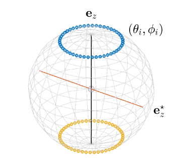
((a))

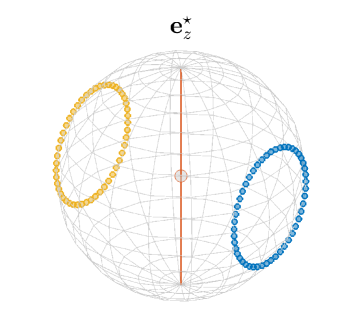
((b))

FIG. 1: An example choice of a new parameterisation in order to avoid coordinate singularities. Shown in blue are the points on the unit sphere corresponding to $(\theta_{i},\phi_{i})$, with their antipodes displayed in yellow. (a) Before a change of basis and subsequent reparameterisation, we see that these points are located near to the $\theta=0$ and $\theta=\pi$ axes, which are shown as black vertical lines. A new potential location for the $\theta=0$ axis is shown in orange, selected so as to maximise the distance from the $(\theta_{i},\phi_{i})$ and their antipodes. (b) Following reparameterisation, the points and antipodes are located maximally away from the new axis. This example scenario corresponds to a helical filament initially with $\theta_{i}=\pi/6$ for $i=1,\ldots,50$.

Initially choosing an arbitrary laboratory basis $\{\bm{e}_{x},\bm{e}_{y},\bm{e}_{z}\}$, the above formulation is implemented in MATLAB^®, with the system of ordinary differential equations (ODEs) of Eq. 37 being solved using the inbuilt stiff ODE solver ode15s, as described in detail by Shampine and Reichelt [27]. This standard variable-step, variable-order solver allows for configurable error tolerances, typically set here at $10^{-5}$ for absolute error and $10^{-4}$ for relative error, in general significantly below the error associated with the piecewise-linear filament discretisation. Derivatives with respect to arclength are approximated with fourth order finite differences, with the resulting dynamics insensitive to this choice of scheme. Initially and at each timestep, the values of $\theta_{i}$ are checked to determine if they are within $\delta$ of a coordinate singularity, typically with $\delta=\pi/50$. Should the parameterisation be approaching a singularity, a new basis is chosen and the problem recast in this basis.

A natural method of selecting a new basis is perhaps to choose one uniformly at random. Indeed, by considering the worst-case scenario of the $N$ tuples $(\theta_{i},\phi_{i})$ uniformly and disjointly covering the surface of the unit sphere, which together $\theta$ and $\phi$ parameterise, the probability that any random basis results in a scenario with $\min_{i}{\{\theta_{i},\pi-\theta_{i}\}}<\delta$ is given by $2N\sin^{2}(\delta/2)$, a consequence of elementary geometry. With this quantity being significantly less than unity for a wide range of $N$ with $\delta$ large enough to avoid severe artificial numerical stiffness, as discussed above, a practical implementation for the simulation of filament elastohydrodynamics as formulated above may simply select a new basis randomly, repeating until a suitable basis is found. With $\delta=\pi/50$ and $N=50$, the probability of rejecting a candidate new basis is bounded above by $10\%$, thus in practice one should expect to find an appropriate basis within few iterations of the proposed procedure.

Alternatively, and as we will do throughout this work, one may instead proceed in a deterministic manner, selecting a near-optimal basis from knowledge of the existing parameterisation. Given the set of parameters $\theta_{i}$ and $\phi_{i}$, we may choose a $\hat{\theta}\in[0,\pi]$ and $\hat{\phi}\in[0,2\pi)$ so as to maximise the distance of $(\hat{\theta},\hat{\phi})$ from each of the $(\theta_{i},\phi_{i})$ and their antipodes. In practice, an approximate solution to this problem is attained by selecting $(\hat{\theta},\hat{\phi})$ from a selection of preset test points in order to maximise the distance from the $(\theta_{i},\phi_{i})$, where distance is measured on the surface of the unit sphere that $\theta$ and $\phi$ naturally parameterise, as shown in Fig. 1. It should be noted that this process of selection impacts negligibly on computational efficiency with 10,000 test points. With these choices of $\hat{\theta}$ and $\hat{\phi}$, we form a new basis by mapping the original basis vector $\bm{e}_{z}$ to the vector $\bm{e}_{z}^{\star}$, given explicitly by

$$\bm{e}_{z}^{\star}=[\sin{\hat{\theta}}\cos{\hat{\phi}},\sin{\hat{\theta}}\sin{\hat{\phi}},\cos{\hat{\theta}}]^{\top}\,.$$ (38)

Choosing the other members of the orthonormal basis $\bm{e}_{x}^{\star},\bm{e}_{y}^{\star}$ arbitrarily, expressed in this new basis the accompanying filament parameterisation will be removed from any coordinate singularities by construction, as exemplified in Fig. 1(b).

III.2 Validation

In what follows we validate the presented methodology against known filament behaviours and a sample three dimensional simulation via an existing methodology. Initial configurations and parameter values for each can be found in the Appendix A, with behaviours qualitatively independent of these parameter choices and filament setups.

III.2.1 Relaxation of a planar filament

Noting there is no analytical test solution for the dynamics of a fully 3D Kirchhoff rod in a viscous fluid, to the best of our knowledge, we consider validations by comparison with numerical studies in the literature, though we additionally utilise invariance of the centre of mass as a gold standard below, where applicable. Firstly, we validate the presented approach by considering the problem of filament relaxation in two dimensions, a natural and well-studied subset of the three dimensional framework. We consider the simple case of a symmetric curved filament in the $\bm{e}_{x}\bm{e}_{y}$ plane, which will provide a test of symmetry preservation, integrated moment balance, and hydrodynamics via qualitative comparisons with the earlier works of Moreau et al. [14] and Hall-Mcnair et al. [15]. Simulating the relaxation of such a filament to a straight equilibrium condition with $N=40$ segments takes less than $2\text{\,}\mathrm{s}$ on modest hardware (Intel^® Core™ i7-6920HQ CPU), from which we immediately see retained the computational efficiency of the framework of Moreau et al. which this work generalises. Present throughout the computed motion is the left-right symmetry of the initial condition, with the filament shape evolving smoothly even with a small number of segments, as shown in Fig. 2. Further, the centre of mass, which in exact calculation would be fixed in space due to the overall force-free condition on the filament, is captured numerically with errors on the order of $10^{-3}L$, demonstrating very good quantitative satisfaction of this condition. Of note, in Fig. 2b we have verified that this error is of the same order of magnitude as that generated by the two-dimensional methodology of Walker et al. [16].

\begin{overpic}[percent,width=433.62pt]{figs/2d_relax/2d_relax.eps} \put(-1.0,22.0){(a)} \put(72.0,22.0){(b)} \end{overpic}

FIG. 2: The two-dimensional relaxation of a symmetric planar filament, simulated with $N=40$ segments. (a) Symmetry is preserved throughout the dynamics, with the relaxation in qualitative agreement with that used for verification in the two-dimensional works of Moreau et al. [14], Hall-Mcnair et al. [15], Walker et al. [16]. (b) Translation of the centre of mass throughout the motion, analytically zero, is captured numerically with errors on the order of $10^{-3}L$ by the proposed methodology, notably the same order of magnitude as that attained with the two-dimensional methodology of Walker et al. [16]. Axes $\bm{x}_{x}$ and $\bm{x}_{y}$ correspond to the unit vectors $\bm{e}_{x}$ and $\bm{e}_{y}$ respectively.

III.2.2 Planar bending of a filament in shear flow

Further, whilst the above is reassuring and serves to validate a subset of the implementation, we note from Eqs. 26 and 27 that motion cast in the $\bm{e}_{x}\bm{e}_{y}$ plane of the laboratory frame may often render the evolution of one of the directors $\bm{d}_{1},\bm{d}_{2}$ trivial. In order to avoid this we may consider planar problems in slightly more generality, posing a problem that is planar though not aligned with the $\bm{e}_{x}\bm{e}_{y}$ plane. As an exemplar such problem we attempt to recreate a typical but complex behaviour of a flexible filament in a shear flow, that of the J-shape and U-turn [28], aligning both the filament and the background flow in a plane spanned by $\bm{e}_{y}$ and $\bm{e}_{x}+\bm{e}_{z}$. In order to ensure the absence of alignment of the parameterisation with the $\bm{e}_{x}\bm{e}_{y}$ plane, we disable the adaptive system of basis selection for the purpose of this example, and simulate the motion of a filament in a shear flow. The background flow with velocity $\bm{u}_{b}$ and vorticity $\bm{\Omega}$ is incorporated into the framework via the transformation $\bm{u}\mapsto\bm{u}-\bm{u}_{b}$, $\omega_{i}\mapsto\omega_{i}-\bm{\Omega}\cdot\bm{d}_{3}^{i}/2$, yielding the modified system

$$-\mathcal{B}\mathcal{A}\mathcal{Q}\dot{\bm{\Theta}}=\bm{R}-\mathcal{B}\mathcal{A}\bm{U}_{b}$$ (39)

for a vector $\hat{\bm{U}_{b}}$ of background flows and vorticities evaluated at segment endpoints and midpoints, respectively. Details of the flow field and initial setup are given in the Appendix A.

Adopting the timescale $T$ to be the inverse of the shearing rate of the flow, we consider a parameter regime in which one would expect to see to formation of J-shape and subsequently a U-turn, defined by their characteristic morphologies in Liu et al. [28, Figure 1, Movies S5, S6] and from which an appropriate parameter choice is obtained. Notably, the impact of thermal noise perturbations is not considered here, in contrast to Liu et al. [28], preventing a quantitative comparison. In Fig. 3 we present the initial, J-shape, and U-turn configurations of the filament as simulated via the proposed methodology, with computation requiring approximately $20\text{\,}\mathrm{s}$ with $N=50$ segments. The simulated filament shapes are in qualitative agreement with those shown in Liu et al. [28, Figure 1], and serve as further validation of the coarse-grained methodology. Notably, enabling the described method of basis selection effectively casts this problem in the $\bm{e}_{x}\bm{e}_{y}$ plane, affording a twofold increase in computational efficiency and highlighting the benefits of adaptive reparameterisation.

\begin{overpic}[permil,width=260.17464pt]{figs/nonplanar_shear/nonplanar_shear.eps} \put(-10.0,420.0){(a)} \put(340.0,420.0){(b)} \put(695.0,420.0){(c)} \end{overpic}

FIG. 3: The planar evolution of a filament in shear, exhibiting a rich and well-documented dynamics. (a) Having aligned both the filament and shear flow in a plane not parallel to the $\bm{e}_{x}\bm{e}_{y}$ plane, with the directors non-trivial in this setup, we simulate the motion of the filament through two distinct morphological transitions: (b) the characteristic J-shape and (c) the subsequent U-turn (cf.  Liu et al. [28, Fig. 1, Movies S5, S6]). We note that the choosing of an improved basis for computation has been disabled for this example, and yields a twofold increase in computational efficiency if enabled. Arrows indicate the direction of the background shear flow. Axes $\bm{x}_{x},\bm{x}_{y},\bm{x}_{z}$ correspond to the unit vectors $\bm{e}_{x},\bm{e}_{y},\bm{e}_{z}$, respectively. The plane containing the filament and the shear flow is shown in grey.

III.2.3 Relaxation of a non-planar filament

Finally, we consider truly non-planar relaxation of filaments in three dimensions. Typical simulations of such a relaxation with $N=50$ segments have a runtime of approximately 10$\mathrm{s}$ on the modest hardware described above, often requiring at most one choice of basis though naturally problem dependent, and provide reasonable accuracy. Thus, even when considering inherently three-dimensional problems we see retained in this methodology the low computational cost of the formulation of Moreau et al. [14], representing significant improvements in computational efficiency over recent studies in three dimensions [19, 20, 21]. This is particularly evident when directly comparing the presented coarse-grained methodology with the results of Ishimoto and Gaffney [21], considering in this case the relaxation of a helical configuration to a straight equilibrium. A side-by-side comparison of the relaxation dynamics as computed by the proposed methodology and that presented in Ishimoto and Gaffney is shown in Fig. 4, noting that the work of Ishimoto and Gaffney [21] considers an actively driven nearly inextensible filament, of which relaxation dynamics are a natural subset. Figure 4 highlights good agreement between methodologies that is in line with the level of accuracy typically afforded by resistive force theories used here, recalling errors logarithmic in the filament aspect ratio. Figure 4e shows a quantitative evaluation of the computed solutions, with the deviation of the filament centre of mass from the initial condition shown as solid black curves for each methodology. With the force-free condition implying that the filament centre of mass should not move throughout the relaxation dynamics, this measured deviation serves as an assessment of the accuracy of both frameworks, with each exhibiting variation only on the order of $10^{-2}L$. Also shown in Fig. 4e is a dimensional measure of the difference between the two computed solutions, here denoted $E(t)$ and defined as the non-negative root of

$$E^{2}(t)=\frac{1}{L}\int\limits_{0}^{L}\mathinner{\!\left\lVert\bm{x}_{P}(s,t)-\bm{x}_{IG}(s,t)\right\rVert}_{2}^{2}\mathop{}\!\mathrm{d}{s}\,,$$ (40)

where $\bm{x}_{P}(s,t)$ and $\bm{x}_{IG}(s,t)$ denote the filament centreline as computed by the proposed methodology and that used by Ishimoto and Gaffney, respectively. Numerically approximating this integral with quadrature and noting that this error is consistently on the order of $10^{-2}L$ throughout the relaxation, we see evidenced good quantitative agreement between the two frameworks, thus validating the proposed methodology. We also remark that the solution of Ishimoto and Gaffney [21] does not perfectly satisfy filament inextensibility, with variation in total length of approximately 1%, which may have some impact on the computed dynamics. Thus, when computing $E(t)$ as defined above, we treat $s\in[0,L]$ as a material parameter, with the differences in position $\bm{x}_{P}(s,t)-\bm{x}_{IG}(s,t)$ therefore capturing discrepancies between the simulated locations of the material point with undeformed arclength $s$ at time $t$, with $s$ not necessarily equal to the deformed arclength in the solution of Ishimoto and Gaffney [21].

In contrast to the agreement between solutions, there is a stark difference between the associated time required for computation. Taking $N=100$ segments and computing until relaxation, the coarse-grained framework calculated the solution in approximately $30\text{\,}\mathrm{s}$ on personal computing hardware with ODE error tolerances of $10^{-5}$, whilst the computations utilising the implementation of Ishimoto and Gaffney required $2.5\text{\,}\mathrm{h}$ on a high performance computing cluster. A thorough investigation of the time required for computation with the presented methodology for various choices of the parameters $\epsilon$ and $N$ is showcased in Fig. 5, from which we note the remarkable performance of this simple implementation across parameter regimes, with the walltime naturally dependent on the discretisation parameter $N$.

\begin{overpic}[percent,width=346.89731pt]{figs/relax/relax.eps} \put(-1.0,53.0){(a)} \put(24.0,53.0){(b)} \put(-1.0,28.0){(c)} \put(24.0,28.0){(d)} \put(59.0,53.0){(e)} \end{overpic}

FIG. 4: The relaxation of a filament in three dimensions. Shown are the results of simulating this motion via (a,b) the proposed framework and (c,d) the methodology presented in Ishimoto and Gaffney [21], in turn heavily based on the work of Olson et al. [19] shown from multiple perspectives at multiple timepoints. In both cases we observe relaxation from a non-planar, helical configuration to a straight filament, and good agreement between the two computed solutions, in particular given the logarithmic accuracy of resistive force theories. (e) A quantitative comparison between the two frameworks, with solid lines showing the Euclidean distance of the filament centre of mass from its initial location, analytically zero by the force-free condition though here on the order of $10^{-2}L$. The dashed curve quantifies the error between the computed solutions, denoted $E$, with the square of this error defined as $E^{2}=\int\mathinner{\!\left\lVert\bm{x}_{P}-\bm{x}_{IG}\right\rVert}_{2}^{2}\mathop{}\!\mathrm{d}{s}/L$, where $\bm{x}_{P}$ and $\bm{x}_{IG}$ are the locations of the filament centreline as computed by the proposed methodology and that used by Ishimoto and Gaffney, respectively. Computation with the presented methodology took approximately $30\text{\,}\mathrm{s}$ on a modest laptop computer, in comparison to the multiple hours required on sophisticated cluster hardware for the methodology of Ishimoto and Gaffney. Here we have simulated filament motion with $N=100$ segments. Axes $\bm{x}_{x},\bm{x}_{y},\bm{x}_{z}$ correspond to the unit vectors $\bm{e}_{x},\bm{e}_{y},\bm{e}_{z}$, respectively.

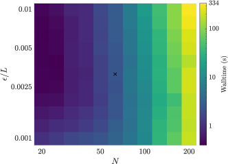
FIG. 5: Walltimes associated with the 3D filament relaxation of Fig. 4 for various choices of the parameters $\epsilon$ and $N$. With $N=200$ corresponding to a very fine discretisation of the filament, we observe a maximum walltime of under 6 minutes on a modest laptop computer, approximately 25x faster than the similar computations of Ishimoto and Gaffney [21] on sophisticated cluster hardware, albeit for different parameter values. There is a strong dependence of the walltime on the level of discretisation, $N$, as expected. Here, the absolute and relative error tolerances of the ODE solver are set to $10^{-5}$ and $10^{-4}$, respectively. All axes, including the colour axis, are logarithmically scaled for visual clarity. For reference, the parameter combination signified by a cross corresponds to a walltime of $2.5\text{\,}\mathrm{s}$, with $N=63$ and $\epsilon/L\approx$3.2\text{\times}{10}^{-3}\text{\,}$$.

III.3 Model extensions

III.3.1 Intrinsic curvature

In order to showcase the versatility of the presented framework, we demonstrate its simple extension to filaments with non-zero intrinsic or reference curvature, which can exhibit complex buckling behaviours [29]. Recalling the constitutive relation of Eq. 8, the effect of an intrinsic curvature $\bm{\kappa}^{0}$ is to alter the bending moments, yielding the modified constitutive relation

$$\bm{m}=EI\left([\kappa_{1}-\kappa_{1}^{0}]\bm{d}_{1}+[\kappa_{2}-\kappa_{2}^{0}]\bm{d}_{2}+\frac{1}{1+\sigma}[\kappa_{3}-\kappa_{3}^{0}]\bm{d}_{3}\right)\,,$$ (41)

where we have written $\bm{\kappa}^{0}=\sum_{\alpha}\kappa_{\alpha}^{0}\bm{d}_{\alpha}$ in the local director basis. Notably, the reference curvature can plausibly depend on a variety of quantities, including time, arclength, and spatial position, with an example being the modelling of an internally driven filament by a time-dependent intrinsic curvature [18, 19].

Practically, the inclusion of such an intrinsic curvature amounts to a simple subtraction of the reference curvature from the computed components of $\bm{\kappa}$ at each instant, with $\bm{R}$ as given in Eq. 20 being modified accordingly. Doing so, we simulate the relaxation of a straight filament with a non-zero intrinsic curvature, with the reference curvature explicitly given by $\bm{\kappa}^{0}=\pi\bm{d}_{2}+2\pi\bm{d}_{3}$ corresponding to a helical configuration. As shown in Fig. 6, the filament indeed relaxes to a helix, with the walltime of this simulation being $15\text{\,}\mathrm{s}$ on a laptop computer, having taken $\epsilon=10^{-2}L$ and $N=70$ segments, noting that the filament shape has been sufficiently resolved with this discretisation.

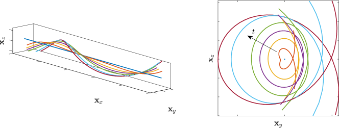
FIG. 6: The relaxation of a straight filament with non-zero intrinsic curvature to a helical configuration, with reference curvature specified as $\bm{\kappa}^{0}=\pi\bm{d}_{2}+2\pi\bm{d}_{3}$. Having taken $N=70$ segments and $\epsilon=10^{-2}L$, we observe the smooth relaxation of the filament away from its initial straight configuration, computed in $15\text{\,}\mathrm{s}$ on a modest laptop computer. Axes $\bm{x}_{x},\bm{x}_{y},\bm{x}_{z}$ correspond to the unit vectors $\bm{e}_{x},\bm{e}_{y},\bm{e}_{z}$, respectively.

III.3.2 Clamped and internally driven filaments

Finally, we consider the simple extensions to both clamped filaments and to those with actively generated internal moments, the latter being akin to the active beating of biological cilia and flagella [30]. For time and arclength-dependent active moment density $\bm{m}^{a}$, its inclusion into the presented framework acts to modify the moment balance of Eq. 2 to

$$\bm{m}_{s}+\bm{x}_{s}\times\bm{n}-\bm{\tau}+\bm{m}^{a}=\bm{0}\,.$$ (42)

Repeating the integration of the pointwise moment balance from $s=s_{i}$ to $s=L$ as in Section II leads to a modified form of Eq. 11, explicitly given as

$$-\bm{d}_{\alpha}^{i}\cdot\left(\bm{I}_{i}^{f}+\bm{I}_{i}^{\tau}\right)=\frac{EI}{1+\delta_{\alpha,3}\sigma}\kappa_{\alpha}(s_{i})-\bm{d}_{\alpha}^{i}\cdot\bm{I}_{i}^{a}\,,$$ (43)

where the integrated active moment density is written as

$$\bm{I}_{i}^{a}=\int\limits_{s_{i}}^{L}\bm{m}^{a}\mathop{}\!\mathrm{d}{\tilde{s}}\,.$$ (44)

For a given active moment density, assumed to be integrable, $\bm{I}_{i}^{a}$ may be readily computed either analytically or numerically, with its components in the local $\bm{d}_{\alpha}^{i}$ direction then modifying $\bm{R}$ from Eq. 20 accordingly.

Clamping the filament at the base is somewhat simpler, in that the overall force and moment balance conditions on the filament are merely replaced by enforcing no motion or rotation at the base. These conditions may be stated concisely as

$$\dot{\bm{x}}(0)=\bm{0}\,,\quad\dot{\theta_{1}}=\dot{\phi_{1}}=\dot{\psi_{1}}=0\,,$$ (45)

supplanting the force and moment-free conditions of Eqs. 5 and 6, having taken $s=0$ in the latter. Implementing these minor modifications, as an example we specify a travelling wave of internal moment given by $\bm{m}^{a}=5\sin(s-t)\bm{d}_{1}+5\cos(s-t)\bm{d}_{2}$ and simulate the active motion of a clamped filament, taking $N=50$ and $\epsilon=10^{-2}L$. Snapshots of this eventually periodic motion are shown in Fig. 7, with the motion simulated up until $t=8\pi$ from a straight initial configuration and with a walltime of around $8\text{\,}\mathrm{s}$.

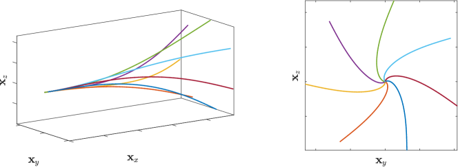
FIG. 7: The 3D beating of a clamped filament driven by prescribed active internal moments. Having specified a travelling wave of out-of-phase sinusoidal active moments $\bm{m}^{a}=5\sin(s-t)\bm{d}_{1}+5\cos(s-t)\bm{d}_{2}$, an initially straight filament deforms to a periodic driven motion, with the tip of the filament following a circular path. Here we have taken $\epsilon=10^{-2}L$ and $N=50$, noting that the filament shape has been resolved smoothly with this level of discretisation. Computation required approximately $8\text{\,}\mathrm{s}$ on modest hardware, simulating up until $t=8\pi$. Axes $\bm{x}_{x},\bm{x}_{y},\bm{x}_{z}$ correspond to the unit vectors $\bm{e}_{x},\bm{e}_{y},\bm{e}_{z}$, respectively.

IV Discussion

In this work we have seen that the motion of inextensible unshearable filaments in three dimensions can be concisely described by a coarse-grained framework, building upon the principles of Moreau et al. [14] in order to minimise numerical stiffness associated with the governing equations of elastohydrodynamics. This representation was readily implemented via an Euler angle parameterisation, with adaptive basis selection and reparameterisation overcoming coordinate singularities associated with a fixed representation of the dynamics. We have further demonstrated the efficacy of the proposed deterministic method for basis selection by explicit simulation of non-planar filament dynamics, which is able to afford reductions in numerical stiffness even when separated from singularities of the parameterisation. The presented framework retains the flexibility and extensibility of the formulations of Moreau et al. [14], Hall-Mcnair et al. [15], Walker et al. [16], with background flows, active moment generation, body forces and other effects or constraints being simple to include in this representation. The simplicity of these possible extensions speaks to the broad utility of the proposed approach, with potential for use in the simulation of both single and multiple filamentous bodies in fluid under a wide variety of circumstances and conditions.

In formulating our methodology we have made the simplifying assumption of coupling fluid dynamics to forces via resistive force theory, which is well-known to incur errors logarithmic in the filament aspect ratio, though variations remain in widespread use [31, 30, 32, 33, 34, 35, 14]. Resistive force theories additionally suffer from locality, in that portions of the filament do not directly interact with one another through the fluid. A natural development of the presented approach would therefore be the inclusion of non-local hydrodynamics, perhaps via the regularised Stokeslet segment methodology of Cortez [36] as included in the work of Walker et al. [16], or lightweight singular slender body theories such as those of Johnson [37], Tornberg and Shelley [4], Walker et al. [38]. Such improvements may also include the consideration of confined geometries, with motion in a half space of particular pertinence to typical microscopy of flagellated organisms. Despite the many possible directions for hydrodynamic refinement, we note that the linearity of Stokes flows necessitates that any relations between forces and velocities be linear, with explicit formulations simply giving rise to modified linear operators $\mathcal{A}$ that may be readily inserted into the described framework.

In the wider context of methods for soft filament simulation, the scope of which is illustrated by the generality of the approach of Gazzola et al. [39], the proposed framework enables rapid simulation of the subclass of purely inextensible filaments. This modeling assumption has been demonstrated to be a valid approximation of nearly inextensible filaments in a variety of contexts [23], affording greatly improved computational efficiency over previous approaches that we have compounded here, albeit with reduced hydrodynamic fidelity. However, we expect that the addition of improved hydrodynamics will have minimal impact on the computational efficiency of the presented methodology, with this efficiency not being derived from our use of simple resistive force theory, as noted by Walker et al. [16], Hall-Mcnair et al. [15] for their non-local refinements of the 2D theory of Moreau et al. [14].

In summary, we have presented, verified and exemplified a novel framework for the rapid simulation of inextensible, unshearable filaments in a viscous fluid at zero Reynolds number. Despite the improved generality of this methodology over existing two-dimensional approaches, we have retained the computational efficiency and simplicity of the work of Moreau et al. [14], affording significant extensibility and thus facilitating a vast range of previously unrealisable biological and biophysical studies into filament dynamics on the microscale.

Appendix A Parameters and initial conditions

We nondimensionalise the system Eq. 37 as in Walker et al. [16], resulting in a dimensionless system of the form

$$-E_{h}\hat{\mathcal{B}}\hat{\mathcal{A}}\hat{\mathcal{Q}}\dot{\hat{\bm{\Theta}}}=\hat{\bm{R}}\,,\quad E_{h}=\frac{8\pi\mu L^{4}}{EI\,T}$$ (46)

for timescale $T$ and elastohydrodynamic number $E_{h}$, where dimensionless counterparts are given by

$$\mathcal{B}=L^{2}\hat{\mathcal{B}}\,,\quad\mathcal{A}=\frac{1}{8\pi\mu}\hat{\mathcal{A}}\,,\quad\mathcal{Q}\dot{\bm{\theta}}=\frac{L}{T}\hat{\mathcal{Q}}\dot{\hat{\bm{\theta}}}\,,\quad\bm{R}=\frac{EI}{L}\hat{\bm{R}}\,,$$ (47)

having multiplied the force balance equations by $\Delta s$ to unify dimensions. All examples begin with the filament base, $\bm{x}_{1}$, coincident with the origin of the laboratory frame, and we set Poisson’s ratio to zero, i.e.  $\sigma=0$ throughout though note a lack of sensitivity of results to this choice.

A.1 Relaxation of a planar filament

In simulating the relaxation of a filament in the $\bm{e}_{x}\bm{e}_{y}$ plane, we impose the initial filament shape as

$$\theta_{i}=\pi/2\,,\quad\phi_{i}=\frac{\pi}{2}\left(\frac{i-1}{N-1}-\frac{1}{2}\right)\,,\quad\psi_{i}=0\,,\quad\text{for }i=1,\ldots,N$$ (48)

with respect to standard laboratory Euler angles. Filament motion is simulated with $E_{h}\approx$1.6\text{\times}{10}^{5}\text{\,}$$, though this choice is arbitrary given the invariance of the dynamics to rescalings in time (assuming that the rescaling is not so extreme as to break the inertialess assumption).

A.2 Planar bending of a filament in shear flow

In order to generate the characteristic behaviours of the J-shape and U-turn we initialise the filament via

$$\theta_{i}=\pi/4\,,\quad\phi_{i}=-\frac{\pi}{12}\frac{i-1}{N-1}\,,\quad\psi_{i}=0\,,\quad\text{for }i=1,\ldots,N\,.$$ (49)

We align a background shear flow in the same plane as the filament, proportional in strength to the coordinate in the $\bm{e}_{y}$ direction, denoted $y$. Explicitly, this flow $\bm{u}_{b}$ is given in the laboratory frame in dimensionless form by

$$\bm{u}_{b}=\frac{1}{\sqrt{2}}y(\bm{e}_{x}+\bm{e}_{z})\,,$$ (50)

having taken the timescale $T$ to be the inverse of the dimensional shear rate. Simulation proceeds with $E_{h}\approx$4.7\text{\times}{10}^{5}\text{\,}$$, consistent with the regime found in Liu et al. [28], and we note that the tip of the filament initially curves into the oncoming background flow in $y<0$.

A.3 Relaxation of a non-planar filament

Taking $N=100$ segments, we impose the helical initial condition

$$\theta_{i}=\pi/3\,,\quad\phi_{i}=2\pi\frac{i-1}{N-1}\,,\quad\psi_{i}=0\,,\quad\text{for }i=1,\ldots,N\,.$$ (51)

We simulate filament motion with $E_{h}\approx$3.1\text{\times}{10}^{4}\text{\,}$$, with results insensitive to this choice. The parameters used in the implementation of Ishimoto and Gaffney [21] are as in their publication, with the image system for a plane wall accordingly removed and the actively generated torques set to zero to allow for filament relaxation in free space. In particular, whilst the filaments of Ishimoto and Gaffney [21] are extensible, the extensional modulus of these filaments is sufficiently high so as to provide near inextensibility in their results, enabling meaningful comparison.

A.4 Relaxation of a non-straight filament

Taking $N=70$ segments, we impose the straight initial condition

$$\theta_{i}=\pi/2\,,\quad\phi_{i}=0\,,\quad\psi_{i}=0\,,\quad\text{for }i=1,\ldots,N\,.$$ (52)

The intrinsic curvature is specified as $\bm{\kappa}^{0}=\pi\bm{d}_{2}+2\pi\bm{d}_{3}$. We simulate filament motion with $E_{h}\approx$1.5\text{\times}{10}^{5}\text{\,}$$, with results insensitive to this choice.

A.5 Active beating of a clamped filament

Taking $N=50$ segments, we impose the straight initial condition

$$\theta_{i}=\pi/2\,,\quad\phi_{i}=0\,,\quad\psi_{i}=0\,,\quad\text{for }i=1,\ldots,N\,.$$ (53)

The active moment density is specified as $\bm{m}^{a}=5\sin(s-t)\bm{d}_{1}+5\cos(s-t)\bm{d}_{2}$. We simulate filament motion with $E_{h}=10^{3}$ up until $t=8\pi$.

References

- Gray [1928] J. Gray, Ciliary movement (Cambridge University Press, Cambridge [England], 1928).
- Hancock [1953] G. J. Hancock, The self-propulsion of microscopic organisms through liquids, Proceedings of the Royal Society of London. Series A. Mathematical and Physical Sciences 217, 96 (1953).
- Berg and Anderson [1973] H. C. Berg and R. A. Anderson, Bacteria swim by rotating their flagellar filaments, Nature 245, 380 (1973).
- Tornberg and Shelley [2004] A. K. Tornberg and M. J. Shelley, Simulating the dynamics and interactions of flexible fibers in Stokes flows, Journal of Computational Physics 196, 8 (2004).
- Roper et al. [2006] M. Roper, R. Dreyfus, J. Baudry, M. Fermigier, J. Bibette, and H. A. Stone, On the dynamics of magnetically driven elastic filaments, Journal of Fluid Mechanics 554, 167 (2006).
- Pozrikidis [2010] C. Pozrikidis, Shear flow over cylindrical rods attached to a substrate, Journal of Fluids and Structures 26, 393 (2010).
- Pozrikidis [2011] C. Pozrikidis, Shear flow past slender elastic rods attached to a plane, International Journal of Solids and Structures 48, 137 (2011).
- Tottori et al. [2012] S. Tottori, L. Zhang, F. Qiu, K. K. Krawczyk, A. Franco-Obregón, and B. J. Nelson, Magnetic helical micromachines: fabrication, controlled swimming, and cargo transport, Advanced Materials 24, 811 (2012).
- Meng et al. [2018] F. Meng, D. Matsunaga, and R. Golestanian, Clustering of Magnetic Swimmers in a Poiseuille Flow, Physical Review Letters 120, 188101 (2018), arXiv:1710.08339 .
- Gray and Hancock [1955] J. Gray and G. J. Hancock, The Propulsion of Sea-Urchin Spermatozoa, Journal of Experimental Biology 32, 802 (1955).
- Johnson [1977] R. E. Johnson, Slender-body theory for Stokes flow and flagellar hydrodynamics, Ph.D. thesis, California Institute of Technology (1977).
- Pozrikidis [1992] C. Pozrikidis, Boundary integral and singularity methods for linearized viscous flow (Cambridge University Press, 1992).
- du Roure et al. [2019] O. du Roure, A. Lindner, E. N. Nazockdast, and M. J. Shelley, Dynamics of Flexible Fibers in Viscous Flows and Fluids, Annual Review of Fluid Mechanics 51, 539 (2019).
- Moreau et al. [2018] C. Moreau, L. Giraldi, and H. Gadêlha, The asymptotic coarse-graining formulation of slender-rods, bio-filaments and flagella, Journal of The Royal Society Interface 15, 20180235 (2018).
- Hall-Mcnair et al. [2019] A. L. Hall-Mcnair, T. D. Montenegro-Johnson, H. Gadêlha, D. J. Smith, and M. T. Gallagher, Efficient implementation of elastohydrodynamics via integral operators, Physical Review Fluids 4, 1 (2019).
- Walker et al. [2019] B. J. Walker, K. Ishimoto, H. Gadêlha, and E. A. Gaffney, Filament mechanics in a half-space via regularised Stokeslet segments, Journal of Fluid Mechanics 879, 808 (2019).
- Yanagimachi [1970] R. Yanagimachi, The movement of golden hamster spermatozoa before and after capacitation, Reproduction 23, 193 (1970).
- Schoeller et al. [2020] S. F. Schoeller, A. K. Townsend, T. A. Westwood, and E. E. Keaveny, Methods for suspensions of passive and active filaments, Journal of Computational Physics , 109846 (2020).
- Olson et al. [2013] S. D. Olson, S. Lim, and R. Cortez, Modeling the dynamics of an elastic rod with intrinsic curvature and twist using a regularized Stokes formulation, Journal of Computational Physics 238, 169 (2013).
- Simons et al. [2015] J. Simons, L. Fauci, and R. Cortez, A fully three-dimensional model of the interaction of driven elastic filaments in a Stokes flow with applications to sperm motility, Journal of Biomechanics 48, 1639 (2015).
- Ishimoto and Gaffney [2018] K. Ishimoto and E. A. Gaffney, An elastohydrodynamical simulation study of filament and spermatozoan swimming driven by internal couples, IMA Journal of Applied Mathematics 83, 655 (2018).
- Bouzarth et al. [2011] E. L. Bouzarth, A. T. Layton, and Y.-N. Young, Modeling a semi-flexible filament in cellular Stokes flow using regularized Stokeslets, International Journal for Numerical Methods in Biomedical Engineering 27, 2021 (2011).
- Jabbarzadeh and Fu [2020] M. Jabbarzadeh and H. C. Fu, A numerical method for inextensible elastic filaments in viscous fluids, Journal of Computational Physics 418, 109643 (2020), arXiv:2003.05608 .
- Antman [2005] S. S. Antman, Nonlinear Problems of Elasticity, Applied Mathematical Sciences, Vol. 107 (Springer-Verlag, New York, 2005).
- Nizette and Goriely [1999] M. Nizette and A. Goriely, Towards a classification of Euler-Kirchhoff filaments, Journal of Mathematical Physics 40, 2830 (1999).
- Chwang and Wu [1974] A. Chwang and T. Y.-T. Wu, Hydromechanics of low-Reynolds-number flow. Part 1. Rotation of axisymmetric prolate bodies, Journal of Fluid Mechanics 63, 607 (1974).
- Shampine and Reichelt [1997] L. F. Shampine and M. W. Reichelt, The MATLAB ODE Suite, SIAM Journal on Scientific Computing 18, 1 (1997).
- Liu et al. [2018] Y. Liu, B. Chakrabarti, D. Saintillan, A. Lindner, and O. du Roure, Morphological transitions of elastic filaments in shear flow, Proceedings of the National Academy of Sciences 115, 9438 (2018).
- Lim [2010] S. Lim, Dynamics of an open elastic rod with intrinsic curvature and twist in a viscous fluid, Physics of Fluids 22, 024104 (2010).
- Gadêlha et al. [2010] H. Gadêlha, E. A. Gaffney, D. J. Smith, and J. C. Kirkman-Brown, Nonlinear instability in flagellar dynamics: a novel modulation mechanism in sperm migration?, Journal of The Royal Society Interface 7, 1689 (2010).
- Lauga et al. [2006] E. Lauga, W. R. DiLuzio, G. M. Whitesides, and H. A. Stone, Swimming in circles: Motion of bacteria near solid boundaries, Biophysical Journal 90, 400 (2006).
- Sznitman et al. [2010] J. Sznitman, X. Shen, R. Sznitman, and P. E. Arratia, Propulsive force measurements and flow behavior of undulatory swimmers at low Reynolds number, Physics of Fluids 22, 121901 (2010).
- Curtis et al. [2012] M. P. Curtis, J. C. Kirkman-Brown, T. J. Connolly, and E. A. Gaffney, Modelling a tethered mammalian sperm cell undergoing hyperactivation, Journal of Theoretical Biology 309, 1 (2012).
- Schulman et al. [2014] R. D. Schulman, M. Backholm, W. S. Ryu, and K. Dalnoki-Veress, Undulatory microswimming near solid boundaries, Physics of Fluids 26, 10.1063/1.4897651 (2014).
- Utada et al. [2014] A. S. Utada, R. R. Bennett, J. C. N. Fong, M. L. Gibiansky, F. H. Yildiz, R. Golestanian, and G. C. L. Wong, Vibrio cholerae use pili and flagella synergistically to effect motility switching and conditional surface attachment, Nature Communications 5, 4913 (2014).
- Cortez [2001] R. Cortez, The method of regularized Stokeslets, SIAM Journal on Scientific Computing 23, 1204 (2001).
- Johnson [1980] R. E. Johnson, An improved slender-body theory for Stokes flow, Journal of Fluid Mechanics 99, 411 (1980).
- Walker et al. [2020] B. J. Walker, M. P. Curtis, K. Ishimoto, and E. A. Gaffney, A regularised slender-body theory of non-uniform filaments, Journal of Fluid Mechanics 899, A3 (2020).
- Gazzola et al. [2018] M. Gazzola, L. H. Dudte, A. G. McCormick, and L. Mahadevan, Forward and inverse problems in the mechanics of soft filaments, Royal Society Open Science 5, 171628 (2018).