Exciton Relaxation in Carbon Nanotubes via Electronic-to-Vibrational Energy Transfer

Abstract

Covalent functionalization of semiconducting single-wall carbon nanotubes (CNT) introduces new photoluminescent emitting states. Theses states are spatially localized at around functionalization sites and strongly red-shifted relative to the emission commonly observed from the nanotube band-edge exciton state. A particularly important feature of these localized exciton states is that, because the exciton is no longer free to diffusively sample photoluminescent quenching sites along the CNT length, its lifetime is significantly extended. We have recently demonstrated that an important relaxation channel of such localized excitons is the electronic-to-vibrational energy transfer (EVET). This process is analogous to the Förster resonance energy transfer (FRET) except the final state of this process is not electronically, but vibrationally excited molecules of the surrounding medium (e.g., solvent). In this work we develop the general theory of EVET, and apply it to the specific case of EVET-mediated relaxation of defect-localized excitons in covalently functionalized CNT. The resulting EVET relaxation times are in good agreement with experimental data.

I Introduction

Covalent functionalization of semiconducting single-wall carbon nanotubes (CNT) by oxygen Ghosh et al. (2010), aryl Piao et al. (2013), and alkyl groups Kwon et al. (2016), with the latter two classes creating sp³ defects, introduces a new photoluminescent (PL) emitting state that is strongly red-shifted from the emission commonly observed from the CNT band-edge exciton state O’Connel et al. (2002). In addition to being the source of new photophysical behaviors, these states are drawing significant interest as the basis for potential emerging functionality such as sensing and imaging Ghosh et al. (2010); Kwon et al. (2015); Shiraki et al. (2016), photon upconversion Akizuki et al. (2015); Maeda et al. (2016), and room-temperature single photon emission Ma et al. (2015); He et al. (2017a). Many of these functionalities arise due to localization of the diffusive band-edge exciton at the defect site Miyauchi et al. (2013); Hartmann et al. (2016); Ma et al. (2014), which in turn leads to significant extension of the exciton lifetime Ma et al. (2015); He et al. (2017a); Miyauchi et al. (2013); Hartmann et al. (2016). This is because the exciton, once trapped at the defect site, is no longer free to diffusively sample PL quenching sites along the length of the carbon nanotube Hertel et al. (2010). Since the long exciton lifetime (hundreds of picoseconds) becomes critical for proposed functionalities, much effort has been directed lately towards understanding the nature of relaxation channels of the trapped exciton in functionalized CNTs Kim et al. (2016); Hartmann et al. (2016); Ma et al. (2017); He et al. (2018). In particular, we have recently suggested that resonance energy transfer between the trapped exciton in CNT and solvent vibrational modes can be an important exciton relaxation channel He et al. (2018).

Electronic-to-vibrational energy transfer (EVET) process, where energy is transferred from an exciton to solvent vibrational degrees of freedom, has been previously shown to be an important exciton relaxation channel in colloidal semiconductor nanoparticles with characteristic EVET times on the order of a few hundred nanoseconds Aharoni et al. (2008); Wen et al. (2016). The prerequisite for EVET is existance of solvent vibrational modes with phonon energies of $\sim 1\,{\rm eV}$. No single fundamental vibrational mode of this energy exists in solvent, but anharmonic effects give rise to the so called overtone and combination modes Falk and Ford (1966); Wen et al. (2016). For example, two representative combination modes in water are $2\nu_{1}+\nu_{3}\approx 9870\,{\rm cm^{-1}\approx}1.22\,{\rm eV}$ and $\nu_{1}+\nu_{2}+\nu_{3}\approx 8250\approx 1.02\,{\rm eV}$, where $\nu_{1}=3261\,{\rm cm^{-1}}$, $\nu_{2}=1639\,{\rm cm}^{-1}$ and $\nu_{3}=3351\,{\rm cm^{-1}}$ are the symmetrical stretching, bending and asymmetrical stretching fundamental vibrational modes, respectively, for ${\rm H_{2}O}$ molecule. Interaction of these modes with external electric field is fully encoded by complex dielectric function, or, equivalently, by the refractive index and absorption coefficient Wen et al. (2016). For example, the existence of these modes is the reason water is not completely transparent in the near-infrared spectral region, so that the absorption coefficient is around $\sim 1\,{\rm cm^{-1}}$ at $\lambda=1150-1300\,{\rm nm}$ He et al. (2018).

In Ref. He et al. (2018) we suggested that relaxation times of a localized exciton in CNTs, associated with EVET, can be as short as $\sim 100-200$ ps. This is significantly faster that that in semiconductor nanoparticles due to much smaller characteristic distances between exciton and absorbing medium for CNTs, $\lesssim 0.5-0.7$ nm He et al. (2018), compared to that of $\approx 3$ nm for semiconductor nanoparticles Aharoni et al. (2008); Wen et al. (2016). The main goal of the present work is to develop a theory for EVET-mediated relaxation of a localized exciton in CNTs. To this end, we first develop a general formalism of EVET, Sec. II. This is done by deriving the effective response function of the exciton-bearing system in the presence of environment, and then extracting the exciton lifetime from the self-energy of the response function. Then, we apply the developed formalism to the cases of (i) simple 1D system near a flat dielectric interface, Sec. III, and (ii) spherical semiconductor nanoparticle, Sec. IV. The latter section, where we re-derive the result previously obtained by Wen et al. Wen et al. (2016), is needed as a sanity check of the general theory. Finally in Sec. V, we obtain a simple closed-form expression for EVET rates for the localized exciton in CNT and estimate the EVET exciton relaxation times at realistic conditions. The resulting times are $\sim 100$ ps, which, considering the level of approximations, is in good agreement with experimentally observed $\tau_{{\rm EVET}}\sim 200$ ps in Ref. He et al. (2018). Section VI concludes.

II General Theory of Resonance Energy Transfer

We split the entire space into two regions assuming that electronic/vibrational wave functions are localized within them, so that the interaction between these regions proceeds only through electromagnetic field. Specific electronic transition $0\leftrightarrow 1$ of energy $E_{10}=\hbar\omega_{10}$ in the first region is designated as the subsystem $I$. All the other (non-resonant) electronic/vibrational transitions in the first region and all the electronic/vibrational transitions in the second region are designated as the subsystem $II$. The response function $\chi$ of some generic system to the external electric potential $V({\bf r},\omega)$ is introduced as

$$\rho({\bf r},\omega)=\int d{\bf r}^{\prime}\,\chi({\bf r},{\bf r}^{\prime};\omega)V({\bf r}^{\prime},\omega),$$ (1)

where $\rho({\bf r},\omega)$ is the induced charge density. Vector variables are typed in bold. The response function for the isolated subsystem $I$ in Lehmann representation is Giuliani and Vignale (2005)

$$\chi_{I}({\bf r},{\bf r}^{\prime};\omega)=\frac{1}{\hbar}\left[\frac{\rho_{01}({\bf r})\rho_{10}({\bf r}^{\prime})}{\omega-\omega_{10}+i\delta}-\frac{\rho_{10}({\bf r})\rho_{01}({\bf r}^{\prime})}{\omega+\omega_{10}+i\delta}\right],$$ (2)

where $\rho_{10}({\bf r})=-e\langle 1|\hat{\varphi}^{\dagger}({\bf r})\hat{\varphi}({\bf r})|0\rangle$ is the transition charge density and $\hat{\varphi}$ ($\hat{\varphi}^{\dagger}$) is the electronic annihilation (creation) field operator. Spin indices are omitted in this work. In what follows we assume a non-magnetic system, so that localized wavefunctions can be chosen real, which in turn yields $\rho_{01}({\bf r})=\rho_{10}({\bf r})$, and therefore

$$\chi_{I}({\bf r},{\bf r}^{\prime};\omega)=\frac{1}{\hbar}\frac{2\omega_{10}}{\omega^{2}-\omega_{10}^{2}+2i\omega\delta}\rho_{10}({\bf r})\rho_{10}({\bf r}^{\prime}).$$ (3)

II.1 Effective response function

Imagine that we are able to fully solve the Poisson problem for the subsystem $II$ so the electrostatic potential at position ${\bf r}$ induced by a unit charge located at ${\bf r}^{\prime}$, fully incorporating the dielectric response of $II$, is given by Green’s function $V_{II}({\bf r},{\bf r}^{\prime};\omega)$. Then, the fully self-consistent charge density induced within subsystem $I$ as a response to external potential $V_{e}({\bf r};\omega)$ acting only on subsystem $I$ is (symbolically) $\rho_{I}=\chi_{I}V_{tot}$, where $V_{tot}=V_{e}+V_{II}\rho_{I}$, resulting in

$$\rho_{I}=\chi_{I}V_{e}+\chi_{I}V_{II}\rho_{I}.$$ (4)

This equation can be solved for the induced charge density as $\rho_{I}=\chi_{I}^{(eff)}V_{e}$, where

$$\chi_{I}^{(eff)}({\bf r},{\bf r}^{\prime};\omega)=\frac{1}{\hbar}\frac{2\omega_{10}\rho_{10}({\bf r})\rho_{10}({\bf r}^{\prime})}{\omega^{2}-\omega_{10}^{2}-2\omega_{10}\Sigma(\omega)/\hbar}$$ (5)

is the effective response function of the subsystem $I$ in the presence of subsystem $II$. Self-energy

$$\Sigma(\omega)=\int d{\bf r}d{\bf r}^{\prime}\,\rho_{10}({\bf r})V_{II}({\bf r},{\bf r}^{\prime};\omega)\rho_{10}({\bf r}^{\prime})$$ (6)

comes from the interaction with subsystem $II$. The real part of self-energy at $\omega=\omega_{0}$ constitutes the energy shift of the $0\leftrightarrow 1$ transition , whereas the imaginary part produces the decay rate of exciton population due to Ohmic losses to the environment (subsystem $II$)

$$\Gamma_{I} =-2\Sigma^{\prime\prime}(\omega_{10})/\hbar$$

$$=-\frac{2}{\hbar}\int d{\bf r}d{\bf r}^{\prime}\,\rho_{10}({\bf r})V_{II}^{\prime\prime}({\bf r},{\bf r}^{\prime};\omega_{10})\rho_{10}({\bf r}^{\prime}),$$ (7)

where double prime stands for the imaginary part.

III 1D system near flat interface

Within the envelope function approximation Yu and Cardona (2005); Haug and Koch (2009), wavefunctions for single-particle electronic states in a semiconductor nanostructure can be represented as $\Psi_{i}({\bf r})=\phi_{i}({\bf r})u_{[i]}({\bf r})$, where $i$ is the state index, and $[i]=c,v$ for $i$ pointing to a state within the conduction or valence band, respectively. Bloch functions $u_{c,v}({\bf r})$ are periodic over the lattice, and envelope functions $\phi_{i}({\bf r})$ vary slowly over the unit cell. Quantum mechanical amplitude for $j\rightarrow i$ transition due to interaction with external potential $V({\bf r})$ is given by $-e\int d{\bf r}\,\Psi_{i}^{*}({\bf r})V({\bf r})\Psi_{j}({\bf r})$. Transition charge density is then naturally introduced as $\rho_{ij}({\bf r})=-e\Psi_{i}^{*}({\bf r})\Psi_{j}({\bf r})$. In the presence of the electron-hole interaction, electron and hole are being scattering within respective bands in the correlated manner, and so the exciton transition density is

$$\rho({\bf r})=\sum_{i\in c}\sum_{j\in v}B_{ij}\rho_{ij}({\bf r})=-e\sum_{i\in c}\sum_{j\in v}B_{ij}\Psi_{i}^{*}({\bf r})\Psi_{j}({\bf r}),$$ (8)

where $B_{ij}$ are the coefficients of expansion of the total exciton wavefunction into the single-particle (electron and hole) ones. These coefficients can generally be found by solving Bethe-Salpeter equation Bechstedt (2015). Explicitly separating slowly and rapidly changing terms, Eq. (8) can be rewritten as

$$\rho({\bf r})=\Phi({\bf r})\rho_{uc}({\bf r})$$ (9)

where the slowly varying exciton envelope wavefunction is normalized as $\int d{\bf r}\,\Phi^{2}({\bf r})=1$, and the lattice-periodic part is $\rho_{uc}({\bf r})\propto u_{c}^{*}({\bf r})u_{v}({\bf r}$). Importantly, integral of $\rho_{uc}$ over the unit cell volume vanishes exactly due to orthogonality of $u_{c}({\bf r})$ and $u_{v}({\bf r})$. However, dipole moment of the unit cell, $\int d{\bf r}\,{\bf r}\rho_{uc}({\bf r})$, does not generally vanish. Exciton transition charge density can thus be thought of as comprising many small transition dipoles, one for each unit cell of the semiconductor.

To develop a general intuition for how the EVET decay rate depends on various geometric parameters of a system, we consider a flat dielectric interface and a simple 1D system whose transition density can be represented by a collection of point charges. The distance between the 1D system and the dielectric interface is $a$ and the transition density of the former is given by

$$\rho(x)=\Phi(x)\rho_{uc}(x),$$ (10)

where $\rho_{uc}(x)=f\sum_{n}\left[\delta(x-b/2-bn)-\delta(x-bn)\right]$ encodes the transition dipole of the unit cell via two point charges. Prefactor $f$ is obtained from setting the total transition dipole moment of the system to $\int dx\,x\rho(x)=d$. Unit cell length is $b$. EVET decay rate near the flat dielectric interface can be evaluated by first finding the Green’s function $V_{II}({\bf r},{\bf r}^{\prime};\omega)$ with the help of the method of image charges, and then substituting this Green’s function into Eq. (7). Accordingly, the dependence of the decay rate on geometry of the system is fully encoded by the following expression

$$I=\sum_{i,j}\frac{Q_{i}Q_{j}}{\sqrt{(x_{i}-x_{j})^{2}+(2a)^{2}}},$$ (11)

where $Q_{i}$ are the point charges constituting the transition density (10), and $x_{i}$ are their positions. In what follows we consider various limiting cases where Eq. (11) can be evaluated analytically or almost analytically. To this end, we consider two possibilities for the exciton envelope function: exponential and Gaussian. Exponential envelope function is given by

$$\Phi(x)=h^{-1/2}e^{-|x|/h},$$ (12)

where $h$ is the characteristic width of the envelope. Its Fourier transform is

$$\Phi_{k}=\int_{-\infty}^{\infty}dx\,\Phi(x)e^{-ikx}=\frac{2h^{1/2}}{1+k^{2}h^{2}}.$$ (13)

The second example is the Gaussian envelope function

$$\Phi(x)=\left(2h\right)^{-1/2}e^{-\frac{\pi x^{2}}{8h^{2}}}$$ (14)

with the Fourier transform

$$\Phi_{k}=\int_{-\infty}^{\infty}dx\,\Phi(x)e^{-iqx}=2h^{1/2}e^{-\frac{2q^{2}h^{2}}{\pi}}.$$ (15)

The numerical prefactor of $\pi/8$ in the exponent of Eq. (14) is chosen intentionally so that $\int dx\,\Phi(k)=\Phi_{k=0}=2h^{1/2}$ is the same for the both envelope functions. Black line in Fig. 1 shows the result of direct numerical evaluation of Eq. (11) for the Gaussian envelope function.

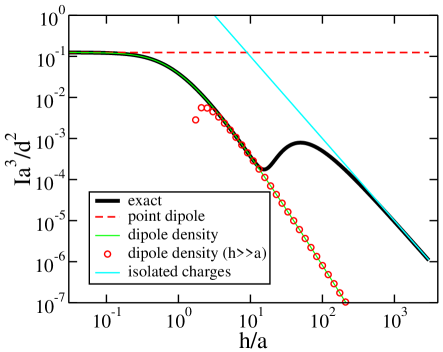
Figure 1: Equation (11), normalized by $d^{2}/a^{3}$, evaluated directly (thick black line) and using various approximation (colored lines and circles) for the Gaussian envelope function. Results for the exponential envelope function are very similar. We set $b=0.1h$.

We set $b=0.1h$ so that there is many units cells within the envelope, otherwise envelope function approximation would break down Yu and Cardona (2005); Haug and Koch (2009).

III.1 $h\gg b\gg a$

In this case, $b\gg a$ and so each transition charge does not interact with images of other charges. Summation in Eq. (11) is then dominated by the diagonal ($i=j$) terms

$$I=\frac{1}{2a}\sum_{i}Q_{i}^{2}.$$ (16)

Since $b=0.1h\ll h$ and, therefore, there is a lot of unit cells within the envelope, summation can be substituted with integration as

$$I=\frac{4d^{2}}{ab}\frac{\int dx\,\Phi^{2}(x)}{\left(\int dx\,\Phi(x)\right)^{2}}=\frac{d^{2}}{abh}.$$ (17)

This expression is plotted as a cyan line in Fig. 1 and is seen to agree well with exact numerical result (black line) at $h/a\gtrsim 200$, or equivalently $b/a\gtrsim 20$. This rather slow convergence to exact results is due to the long-range nature of Coulomb interaction.

III.2 $b\ll a\ll h$

A single transition charge interacts with a large number of image charges at $b\ll a$, and so the summations in Eq. (11) can be substituted with integrations

$$I =\int dx\int dx^{\prime}\,\frac{\rho(x)\rho(x^{\prime})}{\sqrt{(x-x^{\prime})^{2}+(2a)^{2}}}$$

$$=\frac{2}{\pi}\int_{0}^{\infty}dk\,\rho_{-k}\rho_{k}K_{0}(2ka),$$ (18)

where we performed Fourier transformation of the kernel, which yielded modified Bessel function of the second kind $K_{0}$. Dipole moment (or polarization) density $P(x)$ is defined via $\partial_{x}P=-\rho$, or $\rho_{k}=-ikP_{k}$, and so

$$I=\frac{2}{\pi}\int_{0}^{\infty}dk\,k^{2}P_{k}P_{-k}K_{0}(2ka).$$ (19)

Introduction of the dipole moment density is convenient because, first, using definition (10) it is a simple matter to show that $P_{k}$ is exactly proportional to $\Psi_{k}$ if the momentum is not too large ($kb\ll 1$). Secondly, the definition of $P$ implies that $P_{k=0}$ equals the total transition dipole moment $d$. This means that we can directly write $P_{k}=\frac{d}{1+k^{2}h^{2}}$ from Eq. (13) for the exponential envelope function, resulting in

$$I=\frac{2d^{2}}{\pi}\int_{0}^{\infty}dk\,k^{2}\frac{K_{0}(2ka)}{(1+k^{2}h^{2})^{2}}.$$ (20)

For the Gaussian envelope function this equation becomes

$$I=\frac{2d^{2}}{\pi}\int_{0}^{\infty}dk\,k^{2}e^{-4k^{2}h^{2}/\pi}K_{0}(2ka).$$ (21)

This last equation is numerically integrated, yielding thin green line in Fig. 1. As expected, this line agrees with the exact numerical result, when $b$ is smaller than a certain threshold. More specifically, the agreement is already excellent when $b/a\lesssim 1.3$ This is a very important result since it implies that the specific distribution of the transition density within the unit cell is irrelevant, and the continuous and smooth $P(x)\propto\Phi(x)$ can be used when $b\lesssim a$.

Integral in Eq. (20) can be evaluated analytically if we assume $h\gg a$, which allows one to use the small-argument asymptotic form of $K_{0}$ Abramowitz and Stegun (1965)

$$I =-\frac{2d^{2}}{\pi}\int_{0}^{\infty}dk\,\frac{k^{2}\left(\ln ka+\gamma\right)}{(1+k^{2}h^{2})^{2}}$$

$$=\frac{d^{2}}{2h^{3}}\left(\ln\frac{h}{a}-\gamma-1\right),$$ (22)

where $\gamma=0.5772...$ is Euler–Mascheroni constant.

For the gaussian envelope, Eq. (15), one has $P_{k}=de^{-2k^{2}h^{2}/\pi}$, and therefore

$$I =-\frac{2d^{2}}{\pi}\int_{0}^{\infty}dk\,k^{2}e^{-4k^{2}h^{2}/\pi}\left(\ln ka+\gamma\right)$$

$$=\frac{\pi d^{2}}{32h^{3}}\left(\ln\frac{16h^{2}}{\pi a^{2}}-\gamma-2\right).$$ (23)

This last expression is plotted with red circles in Fig. 1. It is seen to agree with (i) Eq. (21) at $h/a\gtrsim 4$ and (ii) exact result (black line) in a window between $h/a\gtrsim 4$ and $h/a\lesssim 13$. This last upper boundary follows of course from $b/a\lesssim 1.3$ condition of applicability of Eq. (21).

III.3 $b,h\ll a$

In this case we effectively have a point dipole interacting with the dielectric interface. Method of image charges is applied and the resulting dipole-dipole interaction energy is Jackson (1998)

$$I=\frac{d^{2}}{(2a)^{3}},$$ (24)

which is plotted as a dashed red horizontal line in Fig. 1 and seed to agree with the exact numerical results at $h/a\lesssim 0.3$.

In the context of above derivations, this expression can also be obtained from Eq. (19) by assuming strongly localized $P(x)$. This results in $k$-independent $P_{k}\approx d$, leading to the same result

$$I=\frac{2}{\pi}d^{2}\int_{0}^{\infty}dk\,k^{2}K_{0}(2ka)=\frac{d^{2}}{(2a)^{3}}.$$ (25)

IV EVET for a quantum dot

In this section we consider the EVET decay rate for a realistic system - spherical semiconductor nanoparticle (quantum dot) of radius $a$ in a solvent. Electrodynamically, it is equivalent to a spherical cavity of radius $a$ with dielectric constants $\epsilon_{in}$ and $\epsilon_{out}$ inside (nanoparticle) and outside (solvent) the cavity, respectively. We have a non-vanishing transition transition charge density $\rho({\bf r})$ only within the cavity and we want to find the corresponding exciton decay rate. The Poisson equation inside is

$$-\Delta\varphi=\frac{4\pi}{\epsilon_{in}}\rho({\bf r}).$$ (26)

Outside, it is the homogenous Poisson (i.e., Laplace) equation, whose solution must be matched to the one inside using the appropriate boundary conditions. To this end, we first expand the transition density into spherical harmonics as

$$\rho({\bf r})=\sum_{l,m}\rho_{lm}(r)Y_{l}^{m}({\bf r}).$$ (27)

Second, we initially assume that $\rho_{lm}(r)=\sigma\delta(r-R)$ where $R<a$. Homogeneous Poisson equation for given spherical symmetry $Y_{l}^{m}$ is

$$\left[-\partial_{r}^{2}-\frac{2}{r}\partial_{r}+\frac{l(l+1)}{r^{2}}\right]\varphi(r)=0.$$ (28)

with solutions $\varphi_{1}=r^{l}$ and $\varphi_{2}=r^{-(l+1)}$. We solve a radial boundary problem with three regions: (I) $r\in(0,R)$, (II) $r\in(R,a)$, (III) $r\in(a,\infty)$. The potential in these three regions are (assuming non-singular behavior at $r\rightarrow 0$ and vanishing potential at $r\rightarrow\infty$)

$$\varphi_{I} =A\varphi_{1}(r),$$ (29)

$$\varphi_{II} =B\varphi_{1}(r)+C\varphi_{2}(r),$$

$$\varphi_{III} =D\varphi_{2}(k),$$

where coefficients $A,B,C,D$ are found from the boundary conditions:

$$A\varphi_{1}(R)=B\varphi_{1}(R)+C\varphi_{2}(R),$$ (30)

$$B\varphi_{1}(a)+C\varphi_{2}(a)=D\varphi_{2}(a),$$

$$\left.\frac{d}{dr}\left(B\varphi_{1}(r)+C\varphi_{2}(r)\right)\right|_{r=R}-\left.\frac{d}{dr}A\varphi_{1}(r)\right|_{r=R}=-4\pi\sigma/\epsilon_{in},$$

$$\epsilon_{in}\left.\frac{d}{dr}\left(B\varphi_{1}(r)+C\varphi_{2}(r)\right)\right|_{r=a}=\epsilon_{out}\left.\frac{d}{dr}D\varphi_{2}(r)\right|_{r=a},$$

where the first two equations match the electrostatic potential at the two boundaries, the third equation encodes the jump of the electric field due to the surface charge at $r=R$, and the last one encodes the jump of the electric field due to the the mismatch of the electric fields due to the induced surface charge on the cavity surface. The resulting coefficients are

$$A =\frac{4\pi\sigma R^{1-l}}{\epsilon_{in}(2l+1)}\left(1+\frac{(1+l)(\epsilon_{in}-\epsilon_{out})}{\epsilon_{out}+l(\epsilon_{in}+\epsilon_{out})}\left(\frac{R}{a}\right)^{2l+1}\right),$$ (31)

$$B =\frac{4\pi\sigma}{\epsilon_{in}(2l+1)}\frac{(1+l)(\epsilon_{in}-\epsilon_{out})}{\epsilon_{out}+l(\epsilon_{in}+\epsilon_{out})}\frac{R^{l+2}}{a^{2l+1}},$$

$$C =\frac{4\pi\sigma}{\epsilon_{in}(2l+1)}R^{l+2},$$

$$D =\frac{4\pi\sigma}{\epsilon_{out}+l(\epsilon_{in}+\epsilon_{out})}R^{l+2}.$$

These coefficients encode both “direct” and “induced” fields. To get the induced fields for e.g., coefficient $A$ we have to evaluate $A^{(ind)}=A-A(\epsilon_{out}\rightarrow\epsilon_{in})$. The result is (for fields inside the cavity)

$$A^{(ind)} =\frac{4\pi\sigma}{\epsilon_{in}(2l+1)}\frac{(1+l)(\epsilon_{in}-\epsilon_{out})}{\epsilon_{out}+l(\epsilon_{in}+\epsilon_{out})}\frac{R^{l+2}}{a^{2l+1}},$$ (32)

$$B^{(ind)} =\frac{4\pi\sigma}{\epsilon_{in}(2l+1)}\frac{(1+l)(\epsilon_{in}-\epsilon_{out})}{\epsilon_{out}+l(\epsilon_{in}+\epsilon_{out})}\frac{R^{l+2}}{a^{2l+1}},$$

$$C^{(ind)} =0.$$

As expected $\varphi_{I}^{(ind)}$ matches smoothly into $\varphi_{II}^{(ind)}$ since induced potential is created by polarization of the interface at $r=a$ and, therefore, do not have a singularity at $r=R$. The resulting induced potential inside the cavity is

$$\varphi^{(ind)}(r)=\frac{4\pi\sigma}{\epsilon_{in}(2l+1)}\frac{(1+l)(\epsilon_{in}-\epsilon_{out})}{\epsilon_{out}+l(\epsilon_{in}+\epsilon_{out})}\frac{R^{l+2}}{a^{2l+1}}r^{l}.$$ (33)

This is the potential from the $r=R$ shell. The full potential is

$$\varphi_{lm}^{(ind)}(r) =\frac{4\pi}{\epsilon_{in}(2l+1)}\frac{(1+l)(\epsilon_{in}-\epsilon_{out})}{\epsilon_{out}+l(\epsilon_{in}+\epsilon_{out})}$$

$$\times\frac{r^{l}}{a^{2l+1}}\int_{0}^{a}dR\,R^{l+2}\rho_{lm}(R).$$ (34)

The self-energy, Eq. (6), for this transition density would be

$$\Sigma =\int_{{\rm cavity}}d{\bf r}\,\rho({\bf r})\varphi^{(ind)}({\bf r})$$

$$=\sum_{l,m}\int_{0}^{a}r^{2}dr\,\rho_{l,-m}(r)\varphi_{lm}^{(ind)}(r).$$ (35)

We now need to discuss how to approximate $\rho({\bf r})$. By performing Fourier transform of transition charge density (8) and discarding large-momentum components corresponding to the internal structure of $u_{c,v}({\bf r})$, one can show that the vector field of transition dipole moment density can be written as ${\bf P}({\bf r})=P({\bf r}){\bf e}_{uc}$. Here, $P({\bf r})\propto\Psi({\bf r})$ - exciton envelope wavefunction, defined in Sec. III, and ${\bf e}_{uc}$ is a unit vector in the direction of the transition dipole of the unit cell, $\int_{uc}d{\bf r}\,{\bf r}u_{c}^{*}({\bf r})u_{v}({\bf r})$. Neglecting the large-momentum components was justified in Sec. III for cases where characteristic distance from the unit cell to the dielectric interface is larger than the unit cell itself. This is true for typical semiconductor quantum dots since their size, and, therefore, typical distance between a unit cell and the dielectric interface, is much larger than the lattice constant Norris (2010). The lowest-energy exciton transition in quantum dots with strong confinement reduces to a product of single-particle electron and hole wavefunctions, whose respective single-particle envelope functions are spherically symmetric Norris (2010). This results in spherically symmetric exciton envelope function $\Phi({\bf r})=\Phi(r)$, and therefore we have

$${\bf P}({\bf r})=P(r){\bf e}_{uc}.$$ (36)

Transition charge density is found from transition dipole moment density as $\rho=-\nabla\cdot{\bf P}$. Orienting ${\bf e}_{uc}$ along $z$-axis in Eq. (36) we find that the expansion of $\rho({\bf r})$ into spherical harmonics, Eq. (27), consists of only a single term of $Y_{1}^{0}$ symmetry. Eq. (35) then becomes

$$\Sigma=\left[\int_{0}^{a}r^{3}dr\,\rho_{1,0}(r)\right]^{2}\frac{8\pi}{3}\frac{\epsilon_{in}-\epsilon_{out}}{\epsilon_{in}+2\epsilon_{out}}\frac{1}{\epsilon_{in}a^{3}}.$$ (37)

The resulting integral in square brackets is exactly proportional to the transition dipole moment $\int_{0}^{a}r^{3}dr\,\rho_{1,0}(r)=\left(\frac{3}{4\pi}\right)^{1/2}d$, so the result for the self-energy is

$$\Sigma=\frac{2(\epsilon_{in}-\epsilon_{out})}{\epsilon_{in}+2\epsilon_{out}}\frac{d^{2}}{\epsilon_{in}a^{3}}.$$ (38)

We further assume that $\epsilon_{in}$ is real and $\epsilon_{out}=\epsilon_{out}^{\prime}+i\epsilon_{out}^{\prime\prime}$, where the imaginary part $\epsilon^{\prime\prime}_{out}$ is small. The resulting decay rate is

$$\Gamma=-2\hbar^{-1}\Sigma^{\prime\prime}=\hbar^{-1}\frac{12\epsilon_{out}^{\prime\prime}}{\left[\epsilon_{in}+2\epsilon_{out}^{\prime}\right]^{2}}\frac{d^{2}}{a^{3}},$$ (39)

where the dielectric constants are to be evaluated at the frequency corresponding to the exciton transition energy. The resulting equation for $\Gamma$ is exactly the same as Eq. (16) in Ref. Wen et al. (2016). The most important observation here is that the substitution of the entire transition charge density distribution with its dipole moment is not an approximation - specific radial distribution of dipole moment density is irrelevant as long as ${\bf P}({\bf r})=P(r){\bf e}_{uc}$. Eq. (39) is thus the same for the both truly point transition dipole located at the center of the spherical cavity, or for the distributed transition dipole of e.g., an electronic transition of a semiconductor quantum dot.

V EVET for Carbon Nanotube

Electrodynamically, an exciton transition in a CNT sitting inside solvent can be treated as follows. There is a cylindrical cavity of radius $a$, dielectric constant inside and outside are $\epsilon_{in}$ and $\epsilon_{out}$, respectively. Radius $a$ is the CNT solvation radius. The transition charge density $\rho(x,\xi)$, technically surface density, resides on a CNT of radius $R<a$ inside the cavity, where $\xi=R\theta$ is the circumferential coordinate. To facilitate the derivation, the charge density is assumed axially periodic with period $L_{x}$, and therefore can be represented by a Fourier series

$$\rho_{k,m}=\int_{0}^{L_{x}}dx\int_{0}^{L_{\xi}}d\xi\,\rho(x,\xi)e^{-ikx}e^{-ik_{\xi}\xi},$$ (40)

where $L_{\xi}=2\pi R$, $k_{\xi}=m/R$ and $k=\frac{2\pi}{L_{x}}n$ so that the inverse transformation looks like

$$\rho(x,\xi)=\frac{1}{L_{x}}\frac{1}{L_{\xi}}\sum_{k}\sum_{m}\rho_{k,m}e^{ikx}e^{im\theta}.$$ (41)

The final result will not depend on $L_{x}$ when it is large. We now want to find an electric potential induced by charge density of specific symmetry $\rho(x,\xi)=\frac{1}{L_{x}L_{\xi}}\rho_{k,m}e^{ikx}e^{ik_{\xi}\xi}$. The homogeneous solution of the Poisson equation within the cylindrical cavity, $\Delta\varphi=0$, is found via expanding into cylindrical harmonics

$$\left(\partial_{r}^{2}+\frac{1}{r}\partial_{r}-k^{2}-\frac{m^{2}}{r^{2}}\right)\varphi=0.$$ (42)

The solutions of this equation are modified Bessel functions of the first, $I_{m}(kr)$, and second, $K_{m}(kr)$, kind, where $k$ and $m$ are understood in the absolute sense, i.e., $k=|k|$ and $m=|m|$. Now we solve a radial boundary problem with three regions: (I) $r\in(0,R)$, (II) $r\in(R,a)$, (III) $r\in(a,\infty)$. The potential in these three regions are (assuming non-singular behavior at $r\rightarrow 0$ and vanishing potential at $r\rightarrow\infty$)

$$\varphi_{I} =AI_{m}(kr),$$ (43)

$$\varphi_{II} =BI_{m}(kr)+CK_{m}(kr),$$

$$\varphi_{III} =DK_{m}(kr),$$

where coefficients $A,B,C,D$ are found from the boundary conditions:

$$AI_{m}(kR)=BI_{m}(kR)+CK_{m}(kR),$$ (44)

$$BI_{m}(ka)+CK_{m}(ka)=DK_{m}(ka),$$

$$\left.\frac{d}{dr}\left(BI_{m}(kr)+CK_{m}(kr)\right)\right|_{r=R}-\left.\frac{d}{dr}AI_{m}(kr)\right|_{r=R}$$

$$=-4\pi\frac{1}{L_{x}L_{\xi}}\rho_{k,m}/\epsilon_{in},$$

$$\epsilon_{in}\left.\frac{d}{dr}\left(BI_{m}(kr)+CK_{m}(kr)\right)\right|_{r=a}=\epsilon_{out}\left.\frac{d}{dr}DK_{m}(kr)\right|_{r=a},$$

where the first two equations match the electrostatic potential at the two boundaries, the third equation encodes the jump of the electric field due to the surface charge at $r=R$, and the last one encodes the jump of the electric field due to the the mismatch of the electric fields due to the induced surface charge on the cavity surface. The exact solution is

$$C_{m}(k) =-\frac{1}{L_{x}L_{\xi}}\frac{4\pi\rho_{k,m}}{\epsilon_{in}k}\frac{I_{m}(kR)}{\mathcal{R}_{m}},$$ (45)

$$B_{m}(k) =-\frac{1}{L_{x}L_{\xi}}\frac{4\pi\rho_{k,m}}{\epsilon_{in}k}\frac{(\epsilon_{out}-\epsilon_{in})I_{m}(kR)K_{m}(ka)K_{m}^{\prime}(ka)}{\mathcal{R}_{m}\mathcal{A}_{m}},$$

$$A_{m}(k) =B_{m}(k)+\frac{K_{m}(kR)}{I_{m}(kR)}C_{m}(k)$$

$$D_{m}(k) =\frac{I_{m}(ka)}{K_{m}(ka)}B_{m}(k)+C_{m}(k),$$

where

$$\mathcal{R}_{m} =I_{m}(kR)K_{m}^{\prime}(kR)-K_{m}(kR)I_{m}^{\prime}(kR)=-\frac{1}{kR},$$ (46)

$$\mathcal{A}_{m} =\epsilon_{in}K_{m}(ka)I_{m}^{\prime}(ka)-\epsilon_{out}I_{m}(ka)K_{m}^{\prime}(ka)$$

$$=\frac{\epsilon_{in}}{ka}-(\epsilon_{out}-\epsilon_{in})I_{m}(ka)K_{m}^{\prime}(ka),$$

where Abel’s identity for modified Bessel functions was used.

The expressions for $A_{m}(k)$, $B_{m}(k)$, $C_{m}(k)$ and $D_{m}(k)$ have contributions from both “direct” and induced potentials. Direct contribution can be found by equating $\epsilon_{out}$ to $\epsilon_{in}$. Induced potential is then found by subtraction. The induced potential at $r=R$ is

$$\varphi^{(ind)}(x,\xi)=B_{m}(k)I_{m}(kR)e^{ikx}e^{ik_{\xi}\xi}$$

$$=-\frac{1}{L_{x}L_{\xi}}\frac{4\pi\rho_{k,m}}{\epsilon_{in}k}\frac{(\epsilon_{out}-\epsilon_{in})I_{m}^{2}(kR)K_{m}(ka)K_{m}^{\prime}(ka)}{\mathcal{R}_{m}\mathcal{A}_{m}}e^{ikx}e^{ik_{\xi}\xi}.$$ (47)

The resulting Fourier transform is

$$\varphi_{k,m}^{(ind)}=-\frac{4\pi\rho_{k,m}}{\epsilon_{in}k}\frac{(\epsilon_{out}-\epsilon_{in})I_{m}^{2}(kR)K_{m}(ka)K_{m}^{\prime}(ka)}{\mathcal{R}_{m}\mathcal{A}_{m}}.$$ (48)

The interaction of the charge density with the potential induced by it reads as, Eq. (6)

$$\Sigma =\int_{0}^{L_{x}}dx\int_{0}^{L_{\xi}}d\xi\,\rho(x,\xi)\varphi^{(ind)}(x,\xi)$$

$$=\int_{0}^{L_{x}}dx\int_{0}^{L_{\xi}}d\xi\,\frac{1}{L_{x}L_{\xi}}\sum_{k,m}\rho_{-k,-m}e^{-ikx}e^{-ik_{\xi}\xi}\varphi^{(ind)}(x,\xi)$$

$$=\frac{1}{L_{x}L_{\xi}}\sum_{k,m}\sigma_{-k,-m}\varphi_{k,m}^{(ind)}.$$ (49)

Using Eq. (48) we have

$$\Sigma =\frac{1}{L_{x}L_{\xi}}\sum_{k,m}\rho_{-k,-m}\varphi_{k,m}^{(ind)}$$

$$=-\frac{1}{L_{x}L_{\xi}}\frac{4\pi(\epsilon_{out}-\epsilon_{in})}{\epsilon_{in}}$$

$$\times\sum_{k,m}\frac{\rho_{k,m}\rho_{-k,-m}}{k}\frac{I_{m}^{2}(kR)K_{m}(ka)K_{m}^{\prime}(ka)}{\mathcal{R}_{m}\mathcal{A}_{m}}.$$ (50)

Slightly rewriting this expression for clarity and better readability

$$\Sigma=\frac{1}{2\pi L_{x}}\sum_{k,m}\rho_{k,m}\rho_{-k,-m}G_{m}(kR,ka),$$ (51)

where

$$G_{m}(x,y)=\frac{4\pi(\epsilon_{out}-\epsilon_{in})}{\epsilon_{in}}\frac{I_{m}^{2}(x)K_{m}(y)K_{m}^{\prime}(y)}{\left[\frac{\epsilon_{in}}{y}-(\epsilon_{out}-\epsilon_{in})I_{m}(y)K_{m}^{\prime}(y)\right]}.$$ (52)

Somewhat similarly to the case of quantum dot above, the transition dipole moment density for a localized exciton in a CNT can be written as

$${\bf P}(x,\xi)=f\Phi(x){\bf e}_{x},$$ (53)

where $\Phi(x)$ is the envelope wavefunction of the localized exciton, and $f$ is the normalizing factor that guarantees that $\int dxd\xi\,{\bf P}(x,\xi)=d{\bf e}_{x}$, where $d$ is the magnitude of total transition dipole moment of the exciton. Detailed derivation is present in Appendix A. Transition charge density is

$$\rho(x,\xi)=-\nabla\cdot{\bf P}(x,\xi)=-fL_{x}^{-1/2}\sum_{k}ikB_{k}e^{ikx},$$ (54)

where

$$B_{k}=L_{x}^{-1/2}\int_{0}^{L_{x}}dx\,\Phi(x)e^{-ikx}$$ (55)

are the Fourier series coefficients for $\Phi(x)$. Accordingly,

$$\rho_{k,m} =\int_{0}^{L_{x}}dx\int_{0}^{L_{\xi}}d\xi\,\rho(x,\xi)e^{-iqx}e^{-ik_{\xi}\xi}$$

$$=-ifL_{x}^{1/2}L_{\xi}kB_{k}\delta_{m,0}.$$ (56)

Substituting this into expression for the self-energy becomes

$$\Sigma=\frac{f^{2}L_{\xi}^{2}}{2\pi}\sum_{q}k^{2}B_{k}B_{-k}G_{0}(kR,ka),$$ (57)

V.1 Delta-functional trap

An important example is a wavefunction for a particle trapped in a delta-function well, Eq (12). The normalization factor is $f=\frac{d}{2h^{1/2}L_{\xi}}$. The resulting self-energy is

$$\Sigma=\frac{d^{2}}{8\pi h}\sum_{k}k^{2}B_{k}B_{-k}G_{0}(kR,ka).$$ (58)

Comparing Eqs. (55) and (13) one has $B_{k}=L_{x}^{-1/2}\frac{2h^{1/2}}{1+k^{2}h^{2}}$ at large $L_{x}$ and so

$$\Sigma=\frac{d^{2}}{2\pi L_{x}}\sum_{k}\frac{k^{2}}{\left(1+k^{2}h^{2}\right)^{2}}G_{0}(kR,ka).$$ (59)

Transforming the summation into integration $\sum_{k}\rightarrow 2\frac{L_{x}}{2\pi}\int_{0}^{\infty}dk$ we obtain

$$\Sigma=\frac{d^{2}}{2\pi^{2}}\int_{0}^{\infty}dk\,\frac{k^{2}}{\left(1+k^{2}h^{2}\right)^{2}}G_{0}(kR,ka),$$ (60)

This integral can be evaluated exactly in the case of point dipole ($h,R\ll a$) in cylindrical cavity with low dielectric constant, $\epsilon_{out}\approx\epsilon_{in}$. In this case, Eq. (52) becomes

$$G_{m}(x,y)=\frac{4\pi(\epsilon_{out}-\epsilon_{in})}{\epsilon_{in}^{2}}yK_{m}(y)K_{m}^{\prime}(y)\delta_{m,0}$$ (61)

and so self-energy (60) reduces to

$$\Sigma =\frac{2(\epsilon_{out}-\epsilon_{in})}{\pi\epsilon_{in}^{2}}\frac{d^{2}}{a^{3}}\int_{0}^{\infty}dy\,y^{3}K_{0}(y)K_{0}^{\prime}(y)$$

$$=-\frac{3\pi^{2}}{32}\frac{(\epsilon_{out}-\epsilon_{in})}{\epsilon_{in}^{2}}\frac{d^{2}}{a^{3}}.$$ (62)

V.2 Gaussian envelope

Another option for the exciton envelope wavefunction is Gaussian, Eq. (14). This Gaussian envelope is chosen so that the normalization factor $f=\frac{d}{2h^{1/2}L_{x}}$ is the same, and, therefore, Eq. (58) applies. Comparing Eqs. (55) and (15) one has $B_{k}=L_{x}^{-1/2}2h^{1/2}e^{-\frac{2q^{2}h^{2}}{\pi}}$ at large $L_{x}$ and so the self-energy becomes

$$\Sigma=\frac{d^{2}}{2\pi^{2}}\int_{0}^{\infty}dk\,k^{2}e^{-\frac{4q^{2}h^{2}}{\pi}}G_{0}(kR,ka).$$ (63)

Clearly, this expression converged to Eq. (62) when $h,R\ll a$ and the low dielectric contrast is small, since in this case the result does not depend on the envelope. Another limiting case is when $h$ is large, so that integration is effectively limited to small momenta. The Poisson kernel becomes

$$G_{0}(kR,ka)=4\pi\frac{\epsilon_{out}-\epsilon_{in}}{\epsilon_{out}\epsilon_{in}}\left(\ln ka/2+\gamma\right).$$ (64)

Integral evaluates exactly, producing

$$\Sigma=-\frac{\pi}{32}\frac{\epsilon_{out}-\epsilon_{in}}{\epsilon_{out}\epsilon_{in}}\frac{d^{2}}{h^{3}}\left(\ln\frac{64h^{2}}{\pi a^{2}}-\gamma-2\right).$$ (65)

If $\epsilon_{out}^{\prime\prime}\ll\epsilon_{out}^{\prime}$, the the EVET decay rate can be written as

$$\Gamma=-2\hbar^{-1}\Sigma^{\prime\prime}=\hbar^{-1}\frac{\pi}{16}\frac{\epsilon_{out}^{\prime\prime}}{\epsilon_{out}^{\prime 2}}\frac{d^{2}}{h^{3}}\left(\ln\frac{64h^{2}}{\pi a^{2}}-\gamma-2\right).$$ (66)

V.3 CNT EVET at realistic conditions

In this subsection, we will evaluate the EVET rate corresponding to a localized exciton in a functionalized CNT. The detailed description of the system is given in our previous work He et al. (2018). Briefly, a chiral (6,5) CNT is assumed to be of radius $R=0.38\,{\rm nm}$ Saito et al. (2000); Alrawashdeh and Lagowski (2018). Distance between CNT surface and the first water solvation shell (for CNTs of similar diameters, but not specifically for (6,5) chirality) is estimated to be $a-R\approx 0.3\,{\rm nm}$ Vijayaraghavan and Wong (2014); Homma et al. (2013), so we estimate the cavity radius as $a=0.68\,{\rm nm}$. CNT is functionalized with 4-methoxybenzene, resulting in the strong localized exciton transition at $\lambda\approx 1160\,{\rm nm}$ with the transition dipole moment of $d=38\,D$ He et al. (2018). The dielectric constant of water at the frequency corresponding to this transition is taken to be $\epsilon_{out}=1.75+i2.7\times 10^{-5}$ He et al. (2018). Exciton localization size in axial direction is typically significantly larger than the CNT radius He et al. (2017b); Gifford et al. (2017). Under these conditions, contributions of the inside of the cavity to the overall dielectric screening is not expected to be too large and can be approximated by a single effective dielectric constant Perebeinos et al. (2004). We assume two different choices for this effective dielectric constant: (i) $\epsilon_{in}=\epsilon_{out}^{\prime}=1.75$ - as if the cavity is filled with water with no absorption, and (ii) $\epsilon_{in}=1$ - “vacuum” cavity. The EVET decay time, $\tau_{{\rm EVET}}=1/\Gamma_{{\rm EVET}}$, for the just overviewed parameters is plotted in Fig. 2 as a function of exciton localization length $h$, assuming Gaussian exciton envelope wavefunction.

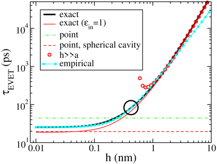
Figure 2: EVET decay time, $\tau_{{\rm EVET}}=1/\Gamma_{{\rm EVET}}$, as a function of exciton localization length $h$. All the results except for the thin red line are plotted for $\epsilon_{in}=1.75$.

Specifically, the results of the numerical integration of Eq. (63) for the first and second choices of $\epsilon_{in}$ are plotted by thick black and thin red lines, respectively. The dielectric screening from inside the cavity becomes expectedly insignificant when $h\gg a$, and so these two lines are seen to coincide at large $h$. This can be further seen from the asymptotic expression for the EVET decay rate at large $h$, Eq. (66), that does not depend on $\epsilon_{in}$ at all. This large-$h$ asymptotic dependence is plotted by red circles and is seen to agree with the exact results when $h\gtrsim 1\,{\rm nm}$. For a point dipole ($R=0$, $h=0$), the EVET decay time for $\epsilon_{in}=1.75$ is shown by the green dashed-dotted line. Red dashed line is the result of evaluation of the EVET time for exactly the same parameters, but assuming a spherical cavity of radius $a$, Eq. (38). Finally, an empirical fit to the exact numerical result for $\epsilon_{in}=1.75$ at not too large $h$ is given by

$$\tau_{EVET}=1.3\tau_{EVET}^{(sphere)}\left[1+5.7(h/a)^{2}\right],$$ (67)

where $\tau_{EVET}^{(sphere)}$ is the EVET decay time for a point dipole in a spherical cavity (dashed red line). This empirical fit is plotted as cyan line in Fig. 2. Parameters $1.3$ and $5.7$ were not obtained from any rigorous fitting procedure, but rather by manually adjusting them until the satisfactory eyeball agreement between the cyan and black lines at $h\lesssim 3\,{\rm nm}$ is reached. These parameters are in principle functions of $R/a$. In particular, at $R\rightarrow 0$, the prefactor of $1.3$ has to be substituted with the one that superimposes cyan and dashed-dotted green lines at $h\rightarrow 0$.

To obtain the exciton localization length $h$ one needs to fit the exciton transition charge density, obtained for example from TD-DFT calculations, with Eq. (12) or Eq. (14). Using exactly this approach we obtained $h\approx 0.54\,{\rm nm}$ and $h\approx 0.43\,{\rm nm}$ for the exponential and Gaussian envelopes, respectively Gifford (2019). This produces the EVET decay times of 120 and 85 ps, respectively, for $\epsilon_{in}=1.75$. In the case of $\epsilon_{in}=1$, the EVET decay rate drops from 85 to 70 ps. The results for $h\approx 0.4\,{\rm nm}$ for the Gaussian envelope are shown by a large black circle in Fig. 2. Experimentally, the EVET decay rate in water was estimated to be $\approx 200\,{\rm ps}$ in Ref. He et al. (2018). Considering the level of approximations in this work, the obtained theoretical result ($\tau_{{\rm EVET}}\sim 100\,{\rm ps}$) is in good agreement with experiment.

VI Conclusion

In this work we developed a general theory of EVET-mediated relaxation of localized excitons in functionalized CNTs. General expressions for the EVET rate, as well as estimates of the EVET exciton relaxation times at realistic conditions were obtained in Sec. V. The specific result, $\tau_{EVET}\sim 100\,{\rm ps}$, is in good agreement with previous experimental results He et al. (2018), considering the level of approximations in this work. The most straightforward way to discuss the level of approximations and the possible approaches to more accurate computations is to consider Eq. (7). In this very general expression, the EVET rate depends on exciton transition charge density and the Green’s function of the electrostatic Poisson equation in the cavity corresponding to the CNT. The former, in the form of the transition dipole moment density (53), was assumed to be a smooth function slowly varying on the scale of the unit cell, and either of exponential or Gaussian envelope. Another, more accurate, approach would be to extract the transition charge density directly from e.g., time-dependent DFT calculations He et al. (2017b); Gifford et al. (2017).

We found the Green’s function of the Poisson equation assuming perfectly cylindrical cavity. This approximation breaks down near the functional group attached to the CNT. The presence of the functional group should somewhat increase the effective solvation radius as solvent molecules cannot be present in the volume occupied by the functional groups. Again, the remedy can come from electronic structure theory calculations, where the Poisson equation is solved routinely for arbitrary shaped cavities within the polarizable continuum model framework Klamt and Schuurmann (1993); Mennucci (2012). An additional complication is the dielectric screening contributed by the CNT itself, which should in principle be incorporated in a non-local and possibly even non-static manner.

Appendix A Transition Charge Density for CNT exciton

Within the 2-band $k\cdot p$ Hamiltonian method, lowest conduction and highest valence band single-particle CNT wavefunctions are ($qR\ll 1$) Ando (2005)

$$\Psi_{c,k_{c}}(x,\xi)=\frac{1}{L_{x}^{1/2}L_{\xi}^{1/2}}\left(u_{c}+\frac{\hbar k_{c}}{\sqrt{2m_{*}\Delta}}u_{v}\right)e^{ik_{c}x}e^{iQ_{x}x+iQ_{\xi}\xi},$$ (68)

$$\Psi_{v,k_{v}}(x,\xi)=\frac{-i}{L_{x}^{1/2}L_{\xi}^{1/2}}\left(u_{v}-\frac{\hbar k_{v}}{\sqrt{2m_{*}\Delta}}u_{c}\right)e^{ik_{v}x}e^{iQ_{x}x+iQ_{\xi}\xi},$$

with corresponding energies $E_{q}=\pm\left(\frac{\Delta}{2}+\frac{\hbar^{2}q^{2}}{2m_{*}}\right)$. Single-particle effective mass and bandgap energy are denoted by $m_{*}$ and $\Delta$, respectively. Bloch function spinors are $u_{c}=[1,0]^{T}$, $u_{v}=[0,1]^{T}$. Constant wavenumbers $Q_{x}$, $Q_{\xi}$ are determined by (i) the CNT chirality, (ii) choice of valley ($K$ or $K^{\prime}$). In what follows, we assume only optically allowed “vertical” exciton transitions so that $Q_{x,\xi}$ does not change upon transition from the valence to conduction band. Spin indices are omitted since the final result does not depend on them. Seemingly unnecessary factor of $-i$ in the valence-band wavefunction in Eq. (68) is added so that the resulting transition density is real (see below).

Within the multi-band envelope function method, the charge density operator is proportional to the unit matrix Velizhanin (2016). Transition charge density, Eq. (8), is then straightforwardly generalized as $\rho(x,\xi)=-e\sum_{k_{c},k_{v}}B_{k_{c}k_{v}}\Psi_{c,k_{c}}^{\dagger}(x,\xi)\sigma_{0}\Psi_{v,k_{v}}(x,\xi)$. Here, $\sigma_{0}$ is $2\times 2$ unit matrix, and the Hermitian conjugation of $\Psi_{c,k_{c}}$ results not only in complex conjugation, but also in transposition of Bloch function spinors, that is e.g., $u_{c}^{\dagger}=[1,0]$ - a row vector. More explicitly, the exciton transition density is

$$\rho(x,\xi)=e\sum_{k_{c},k_{v}}B_{k_{c}k_{v}}\frac{i}{L_{x}L_{\xi}}e^{-i(k_{c}-k_{v})x}\frac{\hbar(k_{c}-k_{v})}{\sqrt{2m_{*}\Delta}},$$ (69)

where coefficients $B_{k_{c}k_{v}}$ can generally be obtained by solving Bethe-Salpeter equation. We, however, first consider a freely propagating exciton of momentum $k$ and assume a simple effective mass approximation where the electron and hole relative motion is hydrogen atom-like and does not depend on the total exciton momentum. Under these conditions, the electron-hole wavefunction for such exciton is $\Psi_{k}(x_{e},x_{h})=L_{x}^{-1/2}L_{\xi}^{-1}\phi_{eh}(x_{e}-x_{h})e^{ik(x_{e}+x_{h})/2}$, where $\phi_{eh}(x_{e}-x_{h})$ encodes the electron and hole axial relative motion in the center-of-mass reference frame, and $e^{ik(x_{e}+x_{h})/2}$ represents the motion of the exciton as the whole. This wavefunction can be expanded into single-particle plane waves as

$$\Psi_{k}(x_{e},x_{h})=\sum_{k_{e},k_{h}}B^{\prime}_{k_{e}k_{h}}\frac{e^{ik_{e}x_{e}}}{L_{x}^{1/2}L_{\xi}^{1/2}}\frac{e^{ik_{h}x_{h}}}{L_{x}^{1/2}L_{\xi}^{1/2}},$$ (70)

so the expansion coefficients are

$$B^{\prime}_{k_{e}k_{h}} =\frac{1}{L_{x}L_{\xi}}\int dx_{e}d\xi_{e}\int dx_{h}d\xi_{h}\,\Psi_{k}(x_{e},x_{h})e^{-ik_{e}x_{e}}e^{-ik_{h}x_{h}}$$

$$=\delta_{k,k_{e}+k_{h}}B^{\prime}_{k_{e}-k/2},$$ (71)

where

$$B^{\prime}_{q}=\frac{1}{L_{x}^{1/2}}\int dx\,\phi_{eh}(x)e^{-iqx}.$$ (72)

Expansion coefficients of the exciton wavefunction into single-particle states in Eqs. (69) and (70) are related as $B_{k_{c}k_{v}}=B^{\prime}_{k_{c},-k_{v}}$, and therefore the transition charge density for the exciton of momentum $k$ becomes

$$\rho_{k}(x,\xi)=e\phi_{eh}(0)\frac{i}{L_{x}^{1/2}L_{\xi}}e^{-ikx}\frac{\hbar k}{\sqrt{2m_{*}\Delta}}$$ (73)

Now, if we consider a localized (by a trap) exciton where the localization is shallow enough to not affect the exciton internal structure and so $\phi_{eh}$ is independent of $k$ in Eq. (73), the transition charge density for this localized exciton is

$$\rho(x,\xi)=\sum_{k}A_{k}^{*}\rho_{k}(x,\xi),$$ (74)

where

$$A_{k}=\frac{1}{L_{x}^{1/2}}\int dx\,\Phi(x)e^{-ikx}$$ (75)

and $\Phi(x)$ is an envelope function of the localized exciton. The function $\Phi(x)$ is real and so $A_{k}=A_{-k}^{*}$. The transition charge density is

$$\rho(x,\xi)=-e\frac{1}{L_{x}^{1/2}L_{\xi}}\phi_{eh}(0)\sum_{k}A_{k}^{*}e^{-ikx}\frac{-i\hbar k}{\sqrt{2m_{*}\Delta}}.$$ (76)

The summation can be represented via the first derivation of $\Phi$ with respect to $x$

$$\rho(x,\xi)=-e\frac{1}{L_{\xi}}\frac{\hbar}{\sqrt{2m_{*}\Delta}}\phi_{eh}(0)\frac{\Phi(x)}{dx}.$$ (77)

Transition dipole moment density is defined as $\rho=-\nabla\cdot{\bf P}$, and so

$${\bf P}(x,\xi)=\frac{1}{L_{\xi}}\frac{\hbar e}{\sqrt{2m_{*}\Delta}}\phi_{eh}(0)\Phi(x){\bf e}_{x},$$ (78)

where ${\bf e}_{x}$ is a unit vector parallel to the $x$-axis. This very simple result means that the transition dipole moment density does not depend on circumferential coordinate $\xi$ and linearly proportional to $\Phi(x)$ - the exciton envelope wavefunction. That ${\bf P}(x,\xi)$ is slowly varying on the scale of the unit cell here can be traced back to the multi-band envelope function $k\cdot p$ approximation, where the transition charge density operator is proportional to the unit matrix and, therefore, the specific local structure of the transition charge density on the scale of single unit cell is averaged over Velizhanin (2016).

References

- Ghosh et al. (2010) S. Ghosh, S. M. Bachilo, R. A. Simonette, K. M. Beckingham, and R. B. Weisman, Science 330, 1656 (2010).
- Piao et al. (2013) Y. Piao, B. Meany, L. R. Powell, N. Valley, H. Kwon, G. C. Schatz, and Y. Wang, Nature Chem. 5, 840 (2013).
- Kwon et al. (2016) H. Kwon, A. Furmanchuk, M. Kim, B. Meany, Y. Guo, G. C. Schatz, and Y. Wang, J. Am. Chem. Soc. 138, 6878 (2016).
- O’Connel et al. (2002) M. J. O’Connel, S. M. Bachilo, C. B. Huffman, V. C. Moore, M. S. Strano, E. H. Haroz, K. L. Rialon, P. J. Boul, W. H. Noon, C. Kittrel, J. Ma, R. H. Hauge, R. B. Weisman, and R. E. Smalley, Science 297, 593 (2002).
- Kwon et al. (2015) H. Kwon, M. Kim, B. Meany, Y. Piao, L. R. Powell, and Y. Wang, J. Phys. Chem. C 119, 3733 (2015).
- Shiraki et al. (2016) T. Shiraki, H. Onitsuka, T. Shiraishi, and N. Nakashima, Chem. Comm. 52, 12972 (2016).
- Akizuki et al. (2015) N. Akizuki, S. Aota, S. Mouri, K. Matsuda, and Y. Miyauchi, Nature Comm. 6, 8920 (2015).
- Maeda et al. (2016) Y. Maeda, S. Minami, Y. Takehana, J. S. Dang, S. Aota, K. Matsuda, Y. Miyauchi, M. Yamada, M. Suzuki, R. S. Zhao, X. Zhao, and S. Nagase, Nanoscale 8, 16916 (2016).
- Ma et al. (2015) X. Ma, N. F. Hartmann, J. K. Baldwin, S. K. Doorn, and H. Htoon, Nature Nanotech. 10, 671 (2015).
- He et al. (2017a) X. He, N. F. Hartmann, X. Ma, Y. Kim, R. Ihly, J. L. Blackburn, W. Gao, J. Kono, Y. Yomogida, A. Hirano, T. Tanaka, H. Kataura, H. Htoon, and S. K. Doorn, Nature Phot. 11, 577 (2017a).
- Miyauchi et al. (2013) Y. Miyauchi, M. Iwamura, S. Mouri, T. Kawazoe, M. Ohtsu, and K. Matsuda, Nature Phot. 7, 715 (2013).
- Hartmann et al. (2016) N. F. Hartmann, K. A. Velizhanin, E. H. Haroz, M. Kim, X. Ma, Y. Wang, H. Htoon, and S. K. Doorn, ACS Nano 10, 8355 (2016).
- Ma et al. (2014) X. Ma, L. Adamska, H. Yamaguchi, S. E. Yalcin, S. Tretiak, S. K. Doorn, and H. Htoon, ACS Nano 8, 10782 (2014).
- Hertel et al. (2010) T. Hertel, S. Himmelein, T. Ackermann, D. Stich, and J. Crochet, ACS Nano 4, 7161 (2010).
- Kim et al. (2016) M. Kim, L. Adamska, N. F. Hartmann, H. Kwon, J. Liu, K. A. Velizhanin, Y. Piao, L. R. Powell, B. Meany, S. K. Doorn, S. Tretiak, and Y. Wang, J. Phys. Chem. C 120, 11268 (2016).
- Ma et al. (2017) X. Ma, N. F. Hartmann, K. A. Velizhanin, J. K. S. Baldwin, L. Adamska, S. Tretiak, S. K. Doorn, and H. Htoon, Nanoscale 9, 16143 (2017).
- He et al. (2018) X. He, K. A. Velizhanin, G. Bullard, Y. Bai, J. H. Olivier, N. F. Hartmann, B. J. Gifford, S. Kilina, S. Tretiak, H. Htoon, M. J. Therien, and S. K. Doorn, ACS Nano 12, 8060 (2018).
- Aharoni et al. (2008) A. Aharoni, D. Oron, U. Banin, E. Rabani, and J. Jortner, Phys. Rev. Lett. 100, 057404 (2008).
- Wen et al. (2016) Q. Wen, S. V. Kershaw, S. Kalytchuk, O. Zhovtiuk, C. Reckmeier, M. I. Vasilevskiy, and A. L. Rogach, ACS Nano 10, 4301 (2016).
- Falk and Ford (1966) M. Falk and T. A. Ford, Can. J. Chem. 44, 1699 (1966).
- Giuliani and Vignale (2005) G. F. Giuliani and G. Vignale, Quantum Theory of the Electron Liquid (Cambridge University Press, Cambridge, UK, 2005).
- Yu and Cardona (2005) P. Y. Yu and M. Cardona, Fundamentals of Semiconductors: Physics and Materials Properties, 2nd ed. (Springer-Verlag, Berlin, 2005).
- Haug and Koch (2009) H. Haug and S. W. Koch, Quantum theory of the optical and electronic properties of semiconductors, 5th ed. (World Scientific, Singapore, 2009).
- Bechstedt (2015) F. Bechstedt, Many-Body Approach to Electronic Excitations: Concepts and Applications, Springer Series in Solid-State Sciences, Vol. 181 (Springer, Heidelberg, Germany, 2015).
- Abramowitz and Stegun (1965) M. Abramowitz and I. A. Stegun, Handbook of Mathematical Functions (Dover, New York, 1965).
- Jackson (1998) J. D. Jackson, Classical Electrodynamics, 3rd ed. (Wiley, New York, 1998).
- Norris (2010) D. J. Norris, “Electronic structure in semiconductor nanocrystals: Optical experiment,” in Nanocrystal Quantum Dots, edited by V. I. Klimov (CRC Press, Boca Raton, FL, 2010) 2nd ed.
- Saito et al. (2000) R. Saito, G. Dresselhaus, and M. S. Dresselhaus, Phys. Rev. B 61, 2981 (2000).
- Alrawashdeh and Lagowski (2018) A. I. Alrawashdeh and J. B. Lagowski, RSC Advances 8, 30520 (2018).
- Vijayaraghavan and Wong (2014) V. Vijayaraghavan and C. H. Wong, Nano-Micro Lett. 6, 268 (2014).
- Homma et al. (2013) Y. Homma, S. Chiashi, T. Yamamoto, K. Kono, D. Matsumoto, J. Shitaba, and S. Sato, Phys. Rev. Lett. 110, 157402 (2013).
- He et al. (2017b) X. He, B. J. Gifford, N. F. Hartmann, R. Ihly, X. Ma, S. V. Kilina, Y. Luo, K. Shayan, S. Strauf, J. L. Blackburn, S. Tretiak, S. K. Doorn, and H. Htoon, ACS Nano 11, 10785 (2017b).
- Gifford et al. (2017) B. J. Gifford, S. Kilina, H. Htoon, S. K. Doorn, and S. Tretiak, J. Phys. Chem. C 122, 1828 (2017).
- Perebeinos et al. (2004) V. Perebeinos, J. Tersoff, and P. Avouris, Phys. Rev. Lett. 92, 257402 (2004).
- Gifford (2019) B. Gifford, unpublished (2019).
- Klamt and Schuurmann (1993) A. Klamt and G. Schuurmann, J. Chem. Soc. Perkin Trans. 2 (1993), 10.1039/p29930000799.
- Mennucci (2012) B. Mennucci, WIREs Comput. Mol. Sci. 2, 386 (2012).
- Ando (2005) T. Ando, J. Phys. Soc. Japan 74, 777 (2005).
- Velizhanin (2016) K. A. Velizhanin, Chem. Phys. 481, 165 (2016).