Joint Radio Resource Allocation and 3D Beam-forming in MISO-NOMA-based Network: Profit Maximization for Mobile Virtual Network Operators

Abstract

Massive connections and high data rate services are key players in 5G ecosystem and beyond. To satisfy the requirements of these types of services, non orthogonal multiple Access (NOMA) and 3-dimensional beam-forming (3DBF) can be exploited. In this paper, we devise a novel radio resource allocation and 3D multiple input single output (MISO) BF algorithm in NOMA-based heterogeneous networks (HetNets) at which our main aim is to maximize the profit of mobile virtual network operators (MVNOs). To this end, we consider multiple infrastructure providers (InPs) and MVNOs serving multiple users. Each InP has multiple access points as base stations (BSs) with specified spectrum and multi-beam antenna array in each transmitter that share its spectrum with MVNO’s users by employing NOMA. To realize this, we formulate a novel optimization problem at which the main aim is to maximize the revenue of MVNOs, subject to resource limitations and quality of service (QoS) constraints. Since our proposed optimization problem is non-convex and mathematically intractable, we transform it into a convex one by introducing a new optimization variable and converting the variables with adopting successive convex approximation. More importantly, the proposed solution is assessed and compared with the alternative search method and the optimal solution that is obtained with adopting the exhaustive search method. In addition, it is studied from the computational complexity, convergence, and performance perspective. Our simulation results demonstrate that NOMA-3DBF has better performance and increases system throughput and MVNO’s revenue compared to orthogonal multiple access with 2DBF by approximately $64$%. Especially, by exploiting 3DBF the MVNO’s revenue is improved nearly $27$% in contrast to 2DBF in high order of antennas.
Index Terms— Resource allocation, MISO, NOMA, 3DBF, optimization, MVNO, revenue, HetNet.

I introduction

I-A State of The Art

With considering exponentially growth of wireless data traffic and diverse novel services such as enhanced mobile broadband, massive internet of thing (mIoT), and critical communication in the fifth generation (5G) of wireless networks, efficient, flexible, and on-demand resource utilization are become very important [1, 2, 3]. To fulfill these services requirements, high frequency band and advanced access technologies are proposed for new radio of 5G access technology [4, 5, 6, 7]. In 5G, due to new emerging services and ultra high density of users, spectral and energy efficiency need be increased significantly. To achieve these goals, advanced physical layer technologies, e.g., high order multi input and multi output (MIMO) and non-orthogonal multiple access (NOMA) are proposed and investigated for 5G [7, 8, 9, 10, 11, 12, 13]. NOMA-based networks have an array of benefits such as high spectral efficiency (SE) and accommodate massive connectivity compared to conventional ones multiple access techniques. Moreover, NOMA reduces radio frequency chains and hardware cost [14, 9]. On the other hand, multiple antennas systems such as multiple input single output (MISO) can significantly improve SE and reliability. In MISO systems, these gains are achieved without increasing the size, cost, and battery life, i.e., the lower level of processing requires less battery consumption at the receivers sides, overally. Exploiting joint NOMA and multiple antennas systems have significant advantages in terms of improving SE by utilizing each resource block more than one in each base station (BS) and applying spatial diversity, respectively [15, 16]. Furthermore, the beam pattern in physical layer has significant impacts on the performance of wireless network; especially for the high losses of propagation at high frequency bands [6]. Three-dimensional beam-forming (3DBF) combining the horizontal and vertical pattern allocation with large number of antennas is one of the most promising technologies for 5G [17, 18, 19, 20, 6]. As studied in [21], interference management is a key limiting factor in increasing the capacity of heterogeneous networks (HetNets). To tackle this issue, by exploiting 3DBF, the vertical and horizontal beams are directed such that the power of intercell interference can be reduced significantly [22]. Moreover, in contrast to two-DBF (2DBF), i.e., just horizontal (azimuth) antenna pattern is adjusted, 3DBF provides tracking of users in both the horizontal and vertical and has negligible side lobes [23].

Nevertheless, combining multiple antennas systems and NOMA with 3DBF can increase SE and capacity of wireless networks multiple times [12] and address heterogeneous service requirements such as, low latency, high data rate, and reliability. Hence, these physical layer technologies are appropriate candidates to address the requirements of 5G and beyond. Accordingly, studying 3DBF in NOMA-based MISO for HetNet from the performance, computational complexity, signaling overhead, and pricing perspectives is the main focus of this paper.

I-B Related Works

Related works on this article can be discussed in the two main categories: 1) NOMA-based MISO networks with various objective functions such as throughput maximization and power consumption minimization; 2) 2DBF and 3DBF in NOMA and (or) MISO-based networks.

I-B1 NOMA-based MISO Networks

Due to the pivotal role of NOMA with MISO on the performance of physical layer of wireless networks, recently, many researches are done in this area [24, 25, 26, 27, 28]. Optimal power allocation for NOMA-based MISO satellite networks with power minimization is proposed in [29]. Robust radio resource allocation in power-domain NOMA (PD-NOMA)-based networks with adopting matching theory is studied in [30]. [31] studies a radio resource allocation in MISO-enabled cloud radio access network. Moreover, energy efficiency for NOMA-based MISO in a single cell network has been studied in [32]. The authors in [10], propose a new power minimization problem in MISO-enabled PD-NOMA-based networks. They consider the minimum rate constraint with steering beam forming and user clustering variables.

I-B2 2DBF and 3DBF in MISO Networks

Up to now, 2DBF and 3DBF multiple antennas systems are received much attention and are studied in many researches from different aspects [33, 34, 35, 15, 36]. The authors in [1] propose BF and power allocation with designing two optimization problems for the terrestrial network. A robust power minimization BF for NOMA-based systems with considering imperfect channel state information (CSI) is studied in [33]. Two dimensional precoding paradigm is applied for 3D massive antennas systems in [25]. In [20], the user experience throughput in relay systems with exploiting 3DBF is evaluated. The authors in [4], study BF in NOMA-based MISO networks with considering two performance metrics, namely, sum data rate and fairness. Two-step BF with considering a multiuser NOMA-based MISO system is proposed in [10]. The first step is a BF nulling to interference reduction at users in power domain superimposed coding cluster and the second step is BF steering for the desired cluster to minimize power utilization.

As can be concluded non of aforementioned works studies joint 3DBF in NOMA-based MISO in multicell networks from the cost and performance perspectives. Moreover, almost all of them consider single cell network [32, 14, 38, 33, 10]. On the other hand, 3DBF is very appropriate choice to reduce interference and losses of propagation at high frequency bands (e.g., mmWave communication) that is desired for 5G and beyond.

I-C Motivations and Contributions

To the best of our knowledge, there is no work on pricing model for 3DBF MISO with the NOMA technique in the HetNet framework. On the other hand, employing both 3DBF in massive antenna systems and NOMA not only have a significant improvement on SE, coverage, etc, but also they can reduce the overall cost of wireless networks, especially in high frequency band communication. These reasons are motivated us to study new pricing models with the joint of 3DBF multi user MISO and NOMA in HetNet by considering infrastructure as a service.

In this paper, we propose a novel joint radio resource allocation, user association, and 3DBF optimization problem with NOMA-based MISO in HetNet. To this end, we consider the case of multi infrastructure providers (InPs) which provide infrastructure as a service for multi mobile virtual network operators (MVNOs) and design a novel pricing-based optimization problem under some constraints. The main aim of the proposed optimization problem is to maximize the revenue of MVNOs’ users subject to the transmit power, subcarrier allocation, successive interference cancellation (SIC), and QoS constraints.

Our main contributions are summarized as follows:

• We propose a new 3D beam and radio resource allocation in downlink of NOMA-based MISO HetNet with proposing a novel pricing model as a mixed integer non-linear programing problem; with aiming to maximize the revenue of MVNOs’ users. We consider multiple InPs that have own physical network and hardware including the BSs that are equipped with multiple transmitters. The InPs server the MVNO’s users based on the service level agreement with MVNOs which is function of cost and revenue. Since our considered framework comprises infrastructure as a service with enabling-virtualization of resources, it is appropriate and applicable to employ network slicing as a key enabler of 5G [39] by considering each MVNO’s resources as a slice.

• We propose three methods, namely, jointly solving continues and integer variables (JS-CIV), alternative search method (ASM), and optimal solution to solve the optimization problem which is non-convex and mathematically intractable. Based on the simulation results, JS-CIV outperforms ASM by approximately $7$% and its the optimality gap is nearly $8$%.

• We investigate the performance of the proposed system under different geographical locations as deployment scenarios, such as indoor hotspot, rural, etc. Moreover, we study 2D and 3D channels from the signaling overhead perspective.

• Our simulation results depict that the cost of power and MVNO’s revenue incorporate the influence of transmission technologies, e.g., 3DBF with order of antennas and multiple access technique.

I-D Paper Organizations

This article is arranged as follows. Section II displays the system model and the problem formulations. Section III presents solution of the problem. The simulation results are presented in Section V. Finally, the concluding remarks of this paper is drawn in Section VI.
Notations: Bold upper and lower case letters denote matrices and vectors, respectively. Transpose and conjugate transpose are indicted by ${(\cdot)}^{T}$ and $(\cdot)^{\dagger}$, respectively. $\|\cdot\|$ represents the Euclidean norm, $|\cdot|$ denotes the absolute value, and $\odot$ indicates Hadamard or element-wise product. $\mathbb{E}\{.\}$ is the expectation operator. $\mathcal{C}$ represents the field of complex numbers. $x_{i}$ denotes the $i$-th entry of vector $\mathbb{x}$ and $\mathbb{0}_{a}$ denotes all zero vector with size $a$. Moreover, $\Re\{.\}$ and $\Im\{.\}$ are the real and imaginary parts of the associated argument, respectively.

II System Model and Problem Formulation

II-A System Model

We consider a scenario with multiple InPs and multiple MVNOs where each MVNO severs its users that are placed on different locations over the total coverage area of the network. In other words, we consider a virtualized case where the physical resources provided by several InPs are divided into several virtual resources each of which can be used by one MVNO. We denote the set of InPs by $i\in\mathcal{I}=\{1,\cdots,I\}$, the set of MVNOs by $v\in\mathcal{V}=\{1,\cdots,V\}$, and the set of macro BSs (MBSs) and femto BSs (FBSs) of InP $i$ by $f_{i}\in\mathcal{F}_{i}=\{0,\cdots,F_{i}\}$, where $f_{i}=0$ is the MBS. Hence, the set of the BSs is $\mathcal{F}=\cup_{i\in\mathcal{I}}\mathcal{F}_{i}$ and $F=|\mathcal{F}|$. A typical example of the considered system model is depicted in Fig.1. As seen, each InP has some BSs that supports users of different MVNOs. Moreover, we consider a central unit as a management system that manages the network centralizely, and solves the considered optimization problem and obtains the corresponding optimization variables. We assume that the BSs are equipped with multiple antennas, i.e., $M_{\text{T}}$ antennas and the receivers are single antenna. We consider that the set of all downlink users are randomly distributed in the network and this set is denoted by $\mathcal{K_{\text{Total}}}=\{1,\cdots,K\}$, which is the union of all MVNOs users, i.e., $\mathcal{K_{\text{Total}}}=\cup_{v\in\mathcal{V}}\mathcal{K}_{v}$. In this paper, we focus on the downlink scenario of 3DBF in NOMA-based MISO HetNet.

Furthermore, we consider that the total bandwidth of each InP $i$, which is non overlapping with the other InPs, i.e., $\text{BW}_{i}$ is divided into $N_{i}$ subcarriers with equal bandwidth. Moreover, we assume that each BS $f_{i}$ of InP $i$ has $N_{i}$ subcarriers. We also suppose that perfect CSI is available at each BS and the channel gain from BS $f_{i}$ to user $k$ over subcarrier $n_{i}$ is denoted by $\textbf{h}_{f_{i},n_{i},k}=[h_{f_{i},n_{i},k}^{m}]\in\mathcal{C}^{M_{\text{T}}\times 1}$. The beam vector assigned by BS $f_{i}$ to user $k$ over subcarrier $n_{i}$ is denoted by $\textbf{w}_{f_{i},n_{i},k}=[w_{f_{i},n_{i},k}^{m}]\in\mathcal{C}^{M_{\text{T}}\times 1}$. The maximum allowable transmit power of each FBS is $P_{\max}^{\text{FBS}}$ and for each MBS is $P_{\max}^{\text{MBS}}$. The other parameters are summarized in Table I.

Table I: Notations and their definitions

Notation	Definition
$\mathcal{K}_{v}$	Set of MVNO $v$ users
$\mathcal{K}_{\text{Total}}$	Set of all users
$\mathcal{N}_{i}$	Set of InPs $i$ subcarriers
$\mathcal{V}$	Set of MVNOs
$\mathcal{I}$	Set of InPs
$\mathcal{F}_{i}$	Set of BSs in InP $i$
$M_{T}$	Number of transmit antennas for each BS
${\rho_{f_{i},n_{i},k}}$	Subcarrier assignment and user association indicator
	for user $k$ on subcarrier $n_{i}$ in BS $f_{i}$
$\gamma_{f_{i},n_{i},k}$	Received SINRof user $k$ on
	subcarrier $n_{i}$ from BS $f_{i}$
$L$	Maximum number of users that can be
	assigned to each subcarrier
${\sigma^{2}_{f_{i},n_{i},k}}$	Noise power at user $k$ on subcarrier $n_{i}$ from BS $f_{i}$
$s_{f_{i},n_{i},k}$	Transmit signal at user $k$ on subcarrier
	$n_{i}$ from BS $f_{i}$
$w_{f_{i},n_{i},k}^{m}$	Beam weight for user $k$ on subcarrier $n_{i}$ in BS $f_{i}$
	on antenna $m$

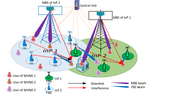
Figure 1: Considered system model.

II-B 2D and 3D Channel Models

In 3D directional channel model, the considered channel gain between BS $f_{i}$ and user $k$ on subcarrier $k$ is formulated as follows [34, 30],

$$\mathbb{h}_{f_{i},n_{i},k}={\beta}_{f_{i},n_{i},k}^{1/2}\bm{\Gamma}_{f_{i},n_{i},k},$$ (1)

where $\bm{\Gamma}_{f_{i},n_{i},k}=[{\Gamma}_{f_{i},n_{i},k}^{m}]$ is small scale fading and $\beta_{f_{i},n_{i},k}$ denotes the large scale channel factor from BS $f_{i}$ to user $k$ over subcarrier $n_{i}$ which is formulated in Section II-B1.

II-B1 3D Channel Model

To formulate the 3D directional large scale fading, i.e., ${\beta}_{f_{i},n_{i},k}$, first, we calculate the horizontal and vertical angles between BS $f_{i}$ and user $k$, respectively, as follows:

$$\varphi_{f_{i},k}(x_{f_{i}},y_{f_{i}})=\arctan\left(\frac{y_{f_{i}}-y_{k}}{x_{f_{i}}-x_{k}}\right),$$ (2)

$$\theta_{f_{i},k}(x_{f_{i}},h_{f_{i}})=\arctan\left(\frac{h_{f_{i}}}{x_{f_{i}}-x_{k}}\right),$$ (3)

where $(x_{f_{i}},y_{f_{i}})$ are 2D coordination of BS $f_{i}$, $h_{f_{i}}$ is the height of BS $f_{i}$, and $(x_{k},y_{k})$ is 2D coordination of user $k\in\mathcal{K_{\text{Total}}}$. In order to obtain the large scale fading, the antenna gain over subcarrier $n_{i}$ from BS $f_{i}$ to user $k$ is calculated by (4), [15],

$$G_{f_{i},n_{i},k}(\varphi_{f_{i},k},\theta_{f_{i},k})=G_{f_{i},n_{i},k}^{\text{Hor}}(\varphi_{f_{i},k})+G_{f_{i},n_{i},k}^{\text{Ver}}(\theta_{f_{i},k}),$$ (4)

where $G_{f_{i},n_{i},k}^{\text{Hor}}(\varphi_{f_{i},k})$ and $G_{f_{i},n_{i},k}^{\text{Ver}}(\theta_{f_{i},k})$ are horizontal and vertical antenna patterns which are given by [8], [35], [17, 40, 34],

$$G_{f_{i},n_{i},k}^{\text{Hor}}=G_{\max,\text{E}}-\min\left(12\left(\frac{\varphi_{f_{i},k}-\hat{\varphi}_{0}}{\hat{\varphi}_{3dB}}\right)^{2},\text{SLL}_{\text{Az}}\right),$$ (5)

$$G_{f_{i},n_{i},k}^{\text{Ver}}=-\min\left(12\left(\frac{\theta_{f_{i},k}-\theta_{f_{i},n_{i},k}^{\text{tilt}}}{\hat{\theta}_{3dB}}\right)^{2},\text{SLL}_{\text{El}}\right),$$ (6)

where $\hat{\varphi}_{3dB}$ and $\hat{\theta}_{3dB}$ depict the half-power beam-width in the azimuth and the elevation patterns, respectively. Whereas $G_{\max,\text{E}}$ is the maximum directional element gain at the antenna bore-sight, $\text{SLL}_{\text{Az}}$ and $\text{SLL}_{\text{El}}$ are the azimuth and elevation slide lobe levels, respectively. Furthermore, $\hat{\varphi}_{0}$ indicates the fixed orientation angle of each BS array boresight relative to the $y$-axis. $\theta_{f_{i},n_{i},k}^{\text{tilt}}$ denotes the optimization variable tilt of BS $f_{i}$ and subcarrier $n_{i}$ for user $k$ which is measured between the direct line passing across the peak of the beam and horizontal plane.

Motivated by the previous discussion, we can formulate the large-scale fading function $\beta_{f_{i},n_{i},k}$ which is composed of path loss and 3D antenna gain and is given by [17, 34]

$$\beta_{f_{i},n_{i},k}=d_{f_{i},k}^{-\varrho}10^{\frac{G_{f_{i},n_{i},k}}{10}},$$ (7)

where $d_{f_{i},k}^{-\varrho}$ expresses the path loss, $d_{f_{i},k}$ is the distance between BS $f_{i}$ and user $k$. Moreover, $\varrho$ is the path loss exponent and $G_{f_{i},n_{i},k}$ represents the gain of antenna and is given by (4).

II-C Radio Resource Allocation

In this section, we formulate the radio resource allocation problem based on the pricing model. To this end, we define the subcarrier assignment and BS selection variable, i.e., $\rho_{f_{i},n_{i},k}\in\{0,1\}$ with $\rho_{f_{i},n_{i},k}=1$, if user $k$ is scheduled to receive information from BS $f_{i}$ over subcarrier $n_{i}$, and otherwise $\rho_{f_{i},n_{i},k}=0$. We assume that the power of information symbol of user $k$ from BS $f_{i}$ over subcarrier $n_{i}$ is denoted by ${s}_{f_{i},n_{i},k}$ is normalized to one, i.e., $\mathbb{E}(|s_{f_{i},n_{i},k}|^{2})=1$. Thus, the signal transmitted by BS $f_{i}$ to user $k$ on subcarrier $n_{i}$ is given by

$$\textbf{x}_{f_{i},n_{i},k}=\rho_{f_{i},n_{i},k}\textbf{w}_{f_{i},n_{i},k}{s}_{f_{i},n_{i},k}.$$ (8)

Note that each user should be assigned to at most one BS. This assumption can be taken into account by the following two constraints:

$$\rho_{f_{i},n_{i},k}+\rho_{f_{j},n_{j},k}\leq 1,\forall i\neq j,i,j\in\mathcal{I},$$

$$n_{i}\in\mathcal{N}_{i},n_{j}\in\mathcal{N}_{j},f_{i},f_{j}\in\mathcal{F},\forall{k}\in\mathcal{K}_{\text{Total}},$$ (9)

$$\rho_{f_{i},n_{i},k}+\rho_{f^{\prime}_{i},n^{\prime}_{i},k}\leq 1,\forall i\in\mathcal{I},\,$$

$$\forall f_{i}\neq f^{\prime}_{i},f_{i},f^{\prime}_{i}\in\mathcal{F}_{i},n_{i},n^{\prime}_{i}\in\mathcal{N}_{i},\forall{k}\in\mathcal{K}_{\text{Total}}.$$ (10)

Constraint (II-C) ensures that each user can be associated to at most one InP’s network and constraint (II-C) guarantees that each user can be assigned to at most one BS that is associated InP. For the subcarrier assignment, based on the NOMA approach in each cell, each subcarrier can be assigned to at most $L$ users. That means, at most $L$ users could be scheduled for each subcarrier based on the following constraint:

$$\sum_{k\in\mathcal{K}}\rho_{f_{i},n_{i},k}\leq L,\forall n_{i}\in\mathcal{N}_{i},f_{i}\in\mathcal{F}_{i},i\in\mathcal{I}.$$ (11)

Based on these definitions, the received signal of user $k$ which is assigned to BS $f_{i}$ for InP $i\in\mathcal{I}$ over subcarrier $n_{i}$ is given by (12),

$$y_{f_{i},n_{i},k}=\underbrace{\textbf{h}^{\dagger}_{f_{i},n_{i},k}\textbf{x}_{f_{i},n_{i},k}}_{\text{a}}+\underbrace{\sum_{k^{\prime}\in\mathcal{K}_{\text{Total}}\backslash k,k^{\prime}\geq k}\textbf{h}^{\dagger}_{f_{i},n_{i},k^{\prime}}\textbf{x}_{f_{i},n_{i},k^{\prime}}}_{\text{b}}+\underbrace{\sum_{f^{\prime}_{i}\in\mathcal{F}_{i},f^{\prime}_{i}\neq f_{i}}\sum_{k^{\prime\prime}\in\mathcal{K}_{\text{Total}}}\textbf{h}^{\dagger}_{f^{\prime}_{i},n_{i},k}\textbf{x}_{f^{\prime}_{i},n_{i},k^{\prime\prime}}}_{\text{c}}+\sigma^{2}_{f_{i},n_{i},k},$$ (12)

 

where (a) is the desired signal and term (b) comes from the NOMA technique which is the interference from users with higher order in SIC ordering and (c) comes from inter-cell interference, respectively. In addition, for the sake of notational simplicity, we use $k^{\prime}\geq k$ to indicate that in SIC ordering, user $k^{\prime}$ has higher order than that of user $k$, i.e., $\mid\textbf{h}^{\dagger}_{f_{i},n_{i},k^{\prime}}\textbf{w}_{f_{i},n_{i},k^{\prime}}\mid^{2}\geq\mid\textbf{h}^{\dagger}_{f_{i},n_{i},k}\textbf{w}_{f_{i},n_{i},k}\mid^{2}$, in the rest of this paper. Moreover, $\sigma^{2}_{f_{i},n_{i},k}$ is the power of additive white Gaussian noise (AWGN). Using these definitions, the SINR of user $k$ is obtained as follows

$$\gamma_{f_{i},n_{i},k}=\frac{\rho_{f_{i},n_{i},k}\mid\textbf{h}^{\dagger}_{f_{i},n_{i},k}\textbf{w}_{f_{i},n_{i},k}\mid^{2}}{\text{Int}_{f_{i},n_{i},k}^{\text{NOMA}}+\text{Int}_{f_{i},n_{i},k}^{\text{Cell}}+\sigma^{2}_{f_{i},n_{i},k}},$$ (13)

where $\text{Int}_{f_{i},n_{i},k}^{\text{NOMA}}$ and $\text{Int}_{f_{i},n_{i},k}^{\text{Cell}}$ are the intra-cell (NOMA) and the inter-cell interference and are given by

$$\text{Int}_{f_{i},n_{i},k}^{\text{NOMA}}=\sum_{k^{\prime}\in\mathcal{K}_{\text{Total}}\backslash k,\,k^{\prime}\geq k}\rho_{f_{i},n_{i},k^{\prime}}\mid\textbf{h}^{\dagger}_{f_{i},n_{i},k}\textbf{w}_{f_{i},n_{i},k^{\prime}}\mid^{2},$$ (14)

$$\text{Int}_{f_{i},n_{i},k}^{\text{Cell}}=\sum_{f^{\prime}_{i}\in\mathcal{F}_{i}\backslash f_{i}}\sum_{k^{\prime\prime}\in\mathcal{K}_{\text{Total}}}\rho_{f^{\prime}_{i},n_{i},k^{\prime\prime}}\mid\textbf{h}^{\dagger}_{f^{\prime}_{i},n_{i},k}\textbf{w}_{f^{\prime}_{i},n_{i},k^{\prime\prime}}\mid^{2},$$ (15)

Therefore, the achievable rate of user $k$ associated with BS $f_{i}$ on subcarrier $n_{i}$ is given by

$$r_{f_{i},n_{i},k}= \sum_{n_{i}\in\mathcal{N}_{i}}\log(1+\gamma_{f_{i},n_{i},k}),\leavevmode\nobreak\ \forall f_{i}\in\mathcal{F}_{i},i\in\mathcal{I},$$

$$k\in\mathcal{K}_{\text{Total}},n_{i}\in\mathcal{N}_{i}.$$ (16)

Hence, the total rate of user $k$ associated with BS $f_{i}$ is $r_{f_{i},k}=\sum_{n_{i}\in\mathcal{N}_{i}}r_{f_{i},n_{i},k}$.

II-D Objective Function and Optimization Problem Formulation

In order to include the cost in the objective function, we assume that each InP charges the MVNOs which are using its infrastructures based on the amount of the resources consumed by the users of these MVNOs. We also assume, the amount of charge of each MVNO $v\in\mathcal{V}$ is proportional to the amount of transmit power consumed by its users, i.e.,

$$C^{\text{Total}}_{v}= \sum_{i\in\mathcal{I}}\sum_{f_{i}\in\mathcal{F}_{i}}\sum_{n_{i}\in\mathcal{N}_{i}}\sum_{k\in\mathcal{K}_{v}}\rho_{f_{i},n_{i},k}C_{i,f_{i}}\|\textbf{w}_{f_{i},n_{i},k}\|^{2},\,$$ (17)

where $C_{i,f_{i}}$ is the amount of charge per unit of power which should be paid when connecting to BS $f_{i}$ in InP $i$. Furthermore, each MVNO charges its users based on the data rate provided to it, and hence, the income of MVNO is given by

$$G^{\text{Total}}_{v}=\sum_{i\in\mathcal{I}}\sum_{f_{i}\in\mathcal{F}_{i}}\sum_{k\in\mathcal{K}_{v}}G_{v,k}r_{f_{i},k},\,\forall v\in\mathcal{V},$$ (18)

where $G_{v,k}$ is the amount of charge per unit of data rate which should be paid to MVNO $v$ by user $k$. Hence, we formulate the revenue of MVNO $v$ as follows

$$U^{\text{Total}}_{v}=G^{\text{Total}}_{v}-C^{\text{Total}}_{v}.$$ (19)

Based on these assumptions and definitions, our proposed optimization problem is maximizing the total revenue of the MVNOs under 3DBF, BS, and subcarrier allocation variables and network constraints is stated as follows:

$$\max_{\mathbb{W},\bm{\rho},\bm{\theta}}O(\mathbb{W},\bm{\rho},\bm{\theta})=\sum_{v\in\mathcal{V}}U^{\text{Total}}_{v}$$ (20a)

$$\mathbb{s.t.}\,\,$$

$$G^{\text{Total}}_{v}\geq C^{\text{Total}}_{v},\forall v\in\mathcal{V},$$ (20b)

$$\gamma_{f_{i},n_{i},k}\geq\gamma_{f_{i},n_{i},k^{\prime}},$$

$$\forall k\geq k^{\prime},\,\forall k\in\mathcal{K}_{\text{Total}},\forall i\in\mathcal{I},f_{i}\in\mathcal{F}_{i},\forall n_{i}\in\mathcal{N}_{i},$$ (20c)

$$\sum_{k\in\mathcal{K}_{\text{Total}}}\sum_{n_{i}\in\mathcal{N}_{i}}\rho_{f_{i},n_{i},k}\|\mathbb{w}_{f_{i},n_{i},k}\|^{2}\leq P_{\max}^{\text{FBS}},$$

$$\forall i\in\mathcal{I},\,f_{i}\in\mathcal{F}_{i},\ f_{i}\neq 0,$$ (20d)

$$\sum_{k\in\mathcal{K}_{\text{Total}}}\sum_{n_{i}\in\mathcal{N}_{i}}\rho_{f_{i},n_{i},k}\|\mathbb{w}_{f_{i},n_{i},k}\|^{2}\leq P_{\max}^{\text{MBS}},$$

$$\forall i\in\mathcal{I},\,f_{i}=0,$$ (20e)

$$\sum_{i\in\mathcal{I}}\sum_{f_{i}\in\mathcal{F}_{i}}\sum_{k\in\mathcal{K}_{v}}\sum_{n_{i}\in\mathcal{N}_{i}}r_{f_{i},n_{i},k}\geq R_{\min}^{v},\,\forall v\in\mathcal{V},$$ (20f)

$$\theta_{f_{i},n_{i},k}^{\text{tilt},\min}\leq\theta_{f_{i},n_{i},k}^{\text{tilt}}\leq\theta_{f_{i},n_{i},k}^{\text{tilt},\max},\,$$

$$\forall i\in\mathcal{I},f_{i}\in\mathcal{F}_{i},\forall n_{i}\in\mathcal{N}_{i},\forall k\in\mathcal{K}_{\text{Total}},$$ (20g)

$$\rho_{f_{i},n_{i},k}+\rho_{f_{j},n_{j},k}\leq 1,\forall i\neq j,i,j\in\mathcal{I},f_{i}\in\mathcal{F}_{i},$$

$$f_{j}\in\mathcal{F}_{j},n_{i}\in\mathcal{N}_{i},n_{j}\in\mathcal{N}_{j},\forall k\in\mathcal{K}_{\text{Total}},$$ (20h)

$$\rho_{f_{i},n_{i},k}+\rho_{f^{\prime}_{i},n^{\prime}_{i},k}\leq 1,\forall f_{i}\neq f^{\prime}_{i},i\in\mathcal{I},$$

$$f_{i},f^{\prime}_{i}\in\mathcal{F}_{i},n_{i},n^{\prime}_{i}\in\mathcal{N}_{i},\forall k\in\mathcal{K}_{\text{Total}},$$ (20i)

$$\sum_{k\in\mathcal{K}_{\text{Total}}}\rho_{f_{i},n_{i},k}\leq L,\forall n_{i}\in\mathcal{N}_{i},f_{i}\in\mathcal{F}_{i},i\in\mathcal{I},$$ (20j)

$$\rho_{f_{i},n_{i},k}\in\{0,1\},\forall n_{i}\in\mathcal{N}_{i},f_{i}\in\mathcal{F}_{i},i\in\mathcal{I},k\in\mathcal{K_{\text{Total}}},$$ (20k)

where $\mathbb{W}=[\mathbb{w}_{f_{i},n_{i},k}]$, $\bm{\rho}=[\rho_{f_{i},n_{i},k}]$, and $\bm{\theta}=[\theta_{f_{i},n_{i},k}^{\text{tilt}}]$. The constraints (20b) and (20) ensure that each MVNO has a benefit and SIC is performed correctly, respectively. The constraints (20) and (20) show the available transmit power budget at each MBS and FBS, respectively. The constraint (20f) guarantees the minimum data rate requirement of each MVNO from QoS perspective. The constraint (20) is used for the upper and lower bounds of 3DBF tilt. The constraints (20)-(20k) are BS selection and subcarrier assignment limitations in which (20) and (20) indicate each user is only assigned to one BS and (20j) demonstrates that each subcarrier can be allocated to at most $L$ users, simultaneously.

III Solution of Optimization Problem

The proposed optimization problem (20) is a non-linear programming problem incorporating both integer and continuous variables. Moreover, due to the non-concavity of the objective function and constraints (20b), (20), and (20f), it is not-convex and intractable. Hence, the well-known convex optimization methods cannot be used, directly. Hence, we propose a new solution method, namely, JS-CIV, which transforms the original non-convex problem into a convex one. To this end, firstly, we introduce new variables, then merge the integer variable with continues variable, and exploit the SCA technique. By these transformations, the well-known traditional sub-optimal solution, i.e., ASM, that is widely applied for solving non-convex and NP-hard problems is not required to solve problem (20). The main two steps of JS-CIV are in the following.

III-A Step-one (Converting and introducing auxiliary variables)

We merge the integer variable (subcarrier and user association), i.e., $\rho_{f_{i},n_{i},k}$ with the 3D beam weighted variable, i.e., $\mathbb{w}_{f_{i},n_{i},k}$ as follows:
Clearly, from (20), (20), and (20k), we obtain that, if $\rho_{f_{i},n_{i},k}=1$, then $\rho_{f^{\prime}_{i},n^{\prime}_{i},k}=0$ and $\rho_{f_{j},n_{j},k}=0,\forall i,j\in{\mathcal{I}},i\neq j,\,f_{i}\neq f^{\prime}_{i}\in\mathcal{F}_{i},n_{i}\in\mathcal{N}_{i},k\in\mathcal{K}_{\text{Total}}$. Therefore, if $\mathbb{w}_{f_{i},n_{i},k}\neq\mathbb{0}_{M_{T}}$ (All zero vector with size $M_{T}$), then $\mathbb{w}_{f^{\prime}_{i},n^{\prime}_{i},k}=\mathbb{0}$ and $\mathbb{w}_{f_{j},n_{j},k}$. Due to the fact that, if subcarrier $n_{i}$ is not allocated to user $k$, then power and beam values on subcarrier $n_{i}$, i.e., $\mathbb{w}_{f_{i},n_{i},k}$ is zero.

Proposition 1.

Assume that $\mathbb{w}_{1}$ and $\mathbb{w}_{2}$ are vectors with complex values and same sizes. Then, we have

$$\mathbb{w}_{1}\odot\mathbb{w}_{2}=\mathbb{0}\Leftrightarrow\mathbb{w}_{1}=\mathbb{0}\leavevmode\nobreak\ \leavevmode\nobreak\ \text{or}\leavevmode\nobreak\ \leavevmode\nobreak\ \mathbb{w}_{2}=\mathbb{0}.$$ (21)

Proof.

To prove this, we consider $z_{1}$ and $z_{2}$ as the elements of $\mathbb{w}_{1}$ and $\mathbb{w}_{2}$, respectively. Meanwhile, we easily can demonstrate that $z_{1}.z_{2}=0\Rightarrow z_{1}=0\leavevmode\nobreak\ \text{or}\leavevmode\nobreak\ z_{2}=0.$ One way to prove is to consider that there exist $z_{1}\neq 0$ and $z_{2}\neq 0$ such that $z_{1}.z_{2}=0$. We infer that $z_{1}=\frac{0}{z_{2}}=0$, is contradiction. This can extend to all elements of $\mathbb{w}_{1}\odot\mathbb{w}_{2}=\mathbb{0}$. ∎

According to the above explanations, the user association constraints (20) and (20) can be replaced by the following continues constraints, equivalently:

$$\mathbb{w}_{f_{i},n_{i},k}\odot\mathbb{w}_{f^{\prime}_{i},n^{\prime}_{i},k}=\mathbb{0},$$

$$\forall i\in\mathcal{I},f_{i}\neq f^{\prime}_{i}\in\mathcal{F}_{i},\,n_{i},n^{\prime}_{i}\in\mathcal{N}_{i},k\in\mathcal{K}_{\text{Total}},$$ (22)

$$\mathbb{w}_{f_{i},n_{i},k}\odot\mathbb{w}_{f_{j},n_{j},k}=\mathbb{0},\forall i\neq j,i,j\in\mathcal{I},f_{i}\in\mathcal{F}_{i},$$

$$f_{j}\in\mathcal{F}_{j},\forall n_{i}\in\mathcal{N}_{i},n_{j}\in\mathcal{N}_{j},\forall k\in\mathcal{K}_{\text{Total}}.$$ (23)

Similarly, based on constraints (20j) and (20k) and assumption of $L=2$, if $\rho_{f_{i},n_{i},k}=1$ and $\rho_{f_{i},n_{i},c}=1$, then, $\rho_{f_{i},n_{i},q}=0,\forall k,c,q\in\mathcal{K}_{\text{Total}},\,q\neq k,q\neq c$. Thus, if $\mathbb{w}_{f_{i},n_{i},k}\neq\mathbb{0}$ and $\mathbb{w}_{f_{i},n_{i},c}\neq\mathbb{0}$, then, $\mathbb{w}_{f_{i},n_{i},q}=\mathbb{0}$. Therefore, the subcarrier assignment constraints (20j) and (20k), equivalently, can be replaced as follows:

$$\big{(}\mathbb{w}_{f_{i},n_{i},k}\odot\mathbb{w}_{f_{i},n_{i},c}\big{)}\odot\mathbb{w}_{f_{i},n_{i},q}=\mathbb{0},$$

$$\forall i\in\mathcal{I},f_{i}\in\mathcal{F}_{i},\,n_{i}\in\mathcal{N}_{i},k,c,q\in\mathcal{K}_{\text{Total}},k\neq c\neq q.$$ (24)

Remark 1.

Note that $L=2$, is more practical and attracted a lot of attentions in both industry [43] and academia [13, 44], [42], [45]. However, we can generalize it to $L=3,4,\dots$ with accepting high complexity by following the same line of the proposed methods. For example, if $L=3$, we have $\Big{(}\big{(}\mathbb{w}_{f_{i},n_{i},k}\odot\mathbb{w}_{f_{i},n_{i},c}\big{)}\odot\mathbb{w}_{f_{i},n_{i},q}\Big{)}\odot{w}_{f_{i},n_{i},g}=\mathbb{0}.$

By the proposed transformation, the integer variable is rewritten as a continues variable by considering its related new constraints. Moreover, to make problem (20) more tractable, we introduce a new slack variable as $\bm{\lambda}=[\lambda_{f_{i},n_{i},k}]$. By this, the rate function (II-C) can be rewritten as $r_{f_{i},n_{i},k}=\log(\lambda_{f_{i},n_{i},k})$. To keep SINR is positive, we should consider that $\lambda_{f_{i},n_{i},k}\geq 0$. Therefore, the original problem (20) can be reformulated as follows [46]:

$$\max_{\mathbb{W},\bm{\theta},\bm{\lambda}}O(\mathbb{W},\bm{\theta},\bm{\lambda})=\sum_{v\in\mathcal{V}}G^{\text{Total}}_{v}-C^{\text{Total}}_{v},$$ (25a)

$$\mathbb{s.t.}$$

$$G^{\text{Total}}_{v}\geq C^{\text{Total}}_{v},\forall v\in\mathcal{V},$$ (25b)

$$\lambda_{f_{i},n_{i},k}\geq 0,\forall i\in\mathcal{I},\forall f_{i}\in\mathcal{F}_{i},\,\forall n_{i}\in\mathcal{N}_{i},\forall k\in\mathcal{K}_{\text{Total}},$$ (25c)

$$1+\gamma_{f_{i},n_{i},k}\geq\lambda_{f_{i},n_{i},k},\forall f_{i}\in\mathcal{F}_{i},\forall n_{i}\in\mathcal{N}_{i},\forall k\in\mathcal{K}_{\text{Total}},$$ (25d)

$$\lambda_{f_{i},n_{i},k}\geq\lambda_{f_{i},n_{i},k^{\prime}},$$

$$\forall k\geq k^{\prime},\,\forall k\in\mathcal{K}_{\text{Total}},\forall i\in\mathcal{I},f_{i}\in\mathcal{F}_{i},\forall n_{i}\in\mathcal{N}_{i},$$ (25e)

$$\sum_{k\in\mathcal{K}_{\text{Total}}}\sum_{n_{i}\in\mathcal{N}_{i}}\|\mathbb{w}_{f_{i},n_{i},k}\|^{2}\leq P_{\max}^{\text{FBS}},\forall i\in\mathcal{I},\,f_{i}\in\mathcal{F}_{i},\ f_{i}\neq 0,$$ (25f)

$$\sum_{k\in\mathcal{K}_{\text{Total}}}\sum_{n_{i}\in\mathcal{N}_{i}}\|\mathbb{w}_{f_{i},n_{i},k}\|^{2}\leq P_{\max}^{\text{MBS}},\forall i\in\mathcal{I},\,f_{i}=0,$$ (25g)

$$\sum_{i\in\mathcal{I}}\sum_{f_{i}\in\mathcal{F}_{i}}\sum_{k\in\mathcal{K}_{v}}\sum_{n_{i}\in\mathcal{N}_{i}}\log(\lambda_{f_{i},n_{i},k})\geq R_{\min}^{v},\,\forall v\in\mathcal{V},$$ (25h)

$$\eqref{bsass},\,\eqref{bsass1},\eqref{subass},\eqref{opttild},$$

where $\mathbb{W}=[\mathbb{w}_{f_{i},n_{i},k}]$, $\bm{\lambda}=[\lambda_{f_{i},n_{i},k}]$, and $\bm{\theta}=[\theta_{f_{i},n_{i},k}^{\text{tilt}}]$. The optimization problem (25) is still non-convex, due to constraints (25d) and (III-A)-(III-A) are non-convex. We convert it into convex one as explained next.

III-B Step-two (Approximation and changing variables)

By substituting (13) into constraint (25d) and some mathematical manipulations, we can rewrite (25d) by (26).

$$\frac{\mid\textbf{h}^{\dagger}_{f_{i},n_{i},k}\textbf{w}_{f_{i},n_{i},k}\mid^{2}}{\big{(}\lambda_{f_{i},n_{i},k}-1\big{)}}\geq\sum_{k^{\prime}\in\mathcal{K}_{\text{Total}}\backslash k,k^{\prime}\succ k}\mid\textbf{h}^{\dagger}_{f_{i},n_{i},k}\textbf{w}_{f_{i},n_{i},k^{\prime}}\mid^{2}+\sum_{f^{\prime}_{i}\in\mathcal{F}_{i}\backslash f_{i}}\sum_{k^{\prime}\in\mathcal{K}_{\text{Total}}\backslash k^{\prime}}\mid\textbf{h}^{\dagger}_{f^{\prime}_{i},n_{i},k}\textbf{w}_{f^{\prime}_{i},n_{i},k^{\prime}}\mid^{2}+{\sigma_{f_{i},n_{i},k}^{2}},$$ (26)

 

In order to convert (26) to a linear constraint, we adopt SCA with first order Taylor series expansion. To this end, we define a new proxy function $g(\Phi_{f_{i},n_{i},k})$ by dividing the product $\textbf{h}^{\dagger}_{f_{i},n_{i},k}\textbf{w}_{f_{i},n_{i},k}$ into the real and imaginary parts as follows [32]:

$$g(\Phi_{f_{i},n_{i},k})\triangleq \mid\textbf{h}^{\dagger}_{f_{i},n_{i},k}\textbf{w}_{f_{i},n_{i},k}\mid^{2}=$$

$$\|[\Re(\textbf{h}^{\dagger}_{f_{i},n_{i},k}\textbf{w}_{f_{i},n_{i},k})\Im(\textbf{h}^{\dagger}_{f_{i},n_{i},k}\textbf{w}_{f_{i},n_{i},k})]^{T}\|^{2},$$ (27)

where $\Phi_{f_{i},n_{i},k}=[\Re(\textbf{h}^{\dagger}_{f_{i},n_{i},k}\textbf{w}_{f_{i},n_{i},k})\Im(\textbf{h}^{\dagger}_{f_{i},n_{i},k}\textbf{w}_{f_{i},n_{i},k})]$. Note that (27) can easily be driven by the corresponding definition. For the sake of notation simplicity, we also define

$$g(\Phi_{f,n,k}^{f^{\prime},n^{\prime},k^{\prime}}) \triangleq\mid\textbf{h}^{\dagger}_{f,n,k}\textbf{w}_{f^{\prime},n^{\prime},k^{\prime}}\mid^{2}.$$ (28)

Now by substituting (28) into (26), we can rewrite (26) by (29).

$$\frac{g(\Phi_{f_{i},n_{i},k}^{(t)})}{\big{(}\lambda_{f_{i},n_{i},k}-1\big{)}}\geq\sum_{k^{\prime}\in\mathcal{K}_{\text{Total}}\backslash k,k^{\prime}\succ k}g(\Phi_{f_{i},n_{i},k}^{f_{i},n_{i},k^{\prime}})+\sum_{f^{\prime}_{i}\in\mathcal{F}_{i}\backslash f_{i}}\sum_{k^{\prime}\in\mathcal{K}_{\text{Total}}\backslash k^{\prime}}g(\Phi_{f_{i},n_{i},k}^{f^{\prime}_{i},n_{i},k^{\prime}})+\sigma^{2}_{f_{i},n_{i},k},$$ (29)

 

Both left and right sides of (29) are non-convex. To tackle this problem, we apply the first order Taylor series expansion to $g(\Phi_{f_{i},n_{i},k})$. With considering two more considerable terms, we can approximate $g(\Phi_{f_{i},n_{i},k})$ at iteration $t$ ($t$ is the iteration number in SCA) by [32]

$$g(\Phi_{f_{i},n_{i},k}^{(t)})\approxeq g(\Phi_{f_{i},n_{i},k}^{(t-1)})+2(\Phi_{f_{i},n_{i},k}^{(t-1)})^{T}\big{[}\Phi_{f_{i},n_{i},k}^{(t)}-\Phi_{f_{i},n_{i},k}^{(t-1)}\big{]}.$$ (30)

Generalized version of (30) according to the definition of (28) is given by (31).

$$g(\Phi_{f,n,k}^{f^{\prime},n^{\prime},k^{\prime},(t)})\approxeq g(\Phi_{f,n,k}^{f^{\prime},n^{\prime},k^{\prime},(t-1)})+2\big{(}\Phi_{f,n,k}^{f^{\prime},n^{\prime},k^{\prime},(t-1)}\big{)}^{T}\big{[}\Phi_{f,n,k}^{f^{\prime},n^{\prime},k^{\prime},(t)}-\Phi_{f,n,k}^{f^{\prime},n^{\prime},k^{\prime},(t-1)}\big{]}.$$ (31)

 

Moreover, we should approximate constraint (29) at point $\lambda_{f_{i},n_{i},k}$ at iteration $t$ as follows:

$$\frac{g(\Phi_{f_{i},n_{i},k}^{(t)})}{\big{(}\lambda_{f_{i},n_{i},k}^{(t)}-1\big{)}} \approxeq\frac{g(\Phi_{f_{i},n_{i},k}^{(t-1)})}{\big{(}\lambda_{f_{i},n_{i},k}^{(t-1)}-1\big{)}}$$

$$-\frac{g(\Phi_{f_{i},n_{i},k}^{(t-1)})}{{(\lambda_{f_{i},n_{i},k}^{(t-1)})}^{2}}[\lambda_{f_{i},n_{i},k}^{(t)}-\lambda_{f_{i},n_{i},k}^{(t-1)}].$$ (32)

By incorporating and applying these approximations into (29), the convexity of constraint (25d) is achievable. Hence, constraint (25d), i.e., (26) (or (29)) is replaced with the proposed linear approximation which is given by (33) in which $g(\Phi_{f_{i},n_{i},k}^{(t)})$ and $\bm{\lambda}^{(t)}=[\lambda_{f_{i},n_{i},k}]$ are updated according to (III-B) and (30), respectively.

$$\frac{g(\Phi_{f_{i},n_{i},k}^{(t-1)})}{\big{(}\lambda_{f_{i},n_{i},k}^{(t-1)}-1\big{)}}-\frac{g(\Phi_{f_{i},n_{i},k}^{(t-1)})}{{(\lambda_{f_{i},n_{i},k}^{(t-1)})}^{2}}[\lambda_{f_{i},n_{i},k}^{(t)}-\lambda_{f_{i},n_{i},k}^{(t-1)}]\geq\sum_{k^{\prime}\in\mathcal{K}_{\text{Total}}\backslash k,k^{\prime}\succ k}\underbrace{g(\Phi_{f_{i},n_{i},k}^{f_{i},n_{i},k^{\prime},(t)})}_{\text{Updated by \eqref{genral_approxteylor}}}+\sum_{f^{\prime}_{i}\in\mathcal{F}_{i}\backslash f_{i}}\sum_{k^{\prime}\in\mathcal{K}_{\text{Total}}\backslash k^{\prime}}\underbrace{g(\Phi_{f_{i},n_{i},k}^{f^{\prime}_{i},n_{i},k^{\prime},(t)})}_{\text{Updated by \eqref{genral_approxteylor}}},$$ (33)

 

For constraints (III-A)-(III-A), we apply the change of variable as defining $\mathbb{w}_{f_{i},n_{i},k}\triangleq\exp(\hat{\mathbb{w}}_{f_{i},n_{i},k})$. Then, by replacing the aforementioned changes and approximations, we have the following optimization problem:

$$\max_{\hat{\mathbb{W}},\bm{\theta},\bm{\lambda}}O(\hat{\mathbb{W}},\bm{\theta},\bm{\lambda}),\,\,\,\,\,$$ (34a)

$$\mathbb{s.t.}\,$$

$$G^{\text{Total}}_{v}\geq C^{\text{Total}}_{v},\forall v\in\mathcal{V},$$ (34b)

$$\sum_{k\in\mathcal{K}_{\text{Total}}}\sum_{n\in N}e^{\|\hat{\mathbb{w}}_{f_{i},n_{i},k}\|^{2}}\leq e^{P_{\max}^{\text{FBS}}},\leavevmode\nobreak\ \forall i\in\mathcal{I},\,f_{i}\in\mathcal{F}_{i},\ f_{i}\neq 0,$$ (34c)

$$\sum_{k\in\mathcal{K}_{\text{Total}}}\sum_{n_{i}\in\mathcal{N}_{i}}e^{\|\hat{\mathbb{w}}_{f_{i},n_{i},k}\|^{2}}\leq e^{P_{\max}^{\text{MBS}}},\,\forall i\in\mathcal{I},\,f_{i}=0,$$ (34d)

$$e^{\hat{\mathbb{w}}_{f_{i},n_{i},k}+\hat{\mathbb{w}}_{f^{\prime}_{i},n^{\prime}_{i},k}}\preceq e^{\mathbb{0}}=\mathbb{1},$$

$$\forall f_{i},f^{\prime}_{i}\in\mathcal{F}_{i},\,n_{i}\in\mathcal{N}_{i},n^{\prime}_{i}\in\mathcal{N}_{i},k\in\mathcal{K}_{\text{Total}},f_{i}\neq f^{\prime}_{i},$$ (34e)

$$e^{\big{(}\hat{\mathbb{w}}_{f_{i},n_{i},k}+\hat{\mathbb{w}}_{f_{j},n_{j},k}\big{)}}\preceq e^{\mathbb{0}}=\mathbb{1},$$

$$\forall f_{i}\in\mathcal{F}_{i}\backslash f^{\prime}_{i},\,n_{i}\in\mathcal{N}_{i},n^{\prime}_{i}\in\mathcal{N}_{i},k\in\mathcal{K}_{\text{Total}},$$ (34f)

$$e^{\big{(}\hat{\mathbb{w}}_{f_{i},n_{i},k}+\hat{\mathbb{w}}_{f_{i},n_{i},c}+\hat{\mathbb{w}}_{f_{i},n_{i},q}\big{)}}\preceq e^{\mathbb{0}}=\mathbb{1},$$

$$\forall f_{i}\in\mathcal{F}_{i},\,n_{i}\in\mathcal{N}_{i},k,c,q\in\mathcal{K}_{\text{Total}},k\neq c\neq q,$$ (34g)

$$\eqref{opttild},\eqref{opt23},\eqref{opt25},\eqref{opt28},\eqref{Final_SCA},$$

where $\mathbb{\hat{\mathbb{W}}}=[\hat{\mathbb{w}}_{f_{i},n_{i},k}]$, $\bm{\lambda}=[\lambda_{f_{i},n_{i},k}]$, $\bm{\theta}=[\theta_{f_{i},n_{i},k}^{\text{tilt}}].$ The optimization problem (34) is convex one and can be solved by utilizing the MATLAB optimization Toolbox such as CVX, efficiently. The main steps of solution (34) is stated in Al. 1.

Input: Initialize $\bm{\Phi}^{0}$ and $\bm{\lambda}^{0}$, set $t=0$, $0<\Upsilon<<1$ is tolerance (or accuracy), and $T$ is the allowable number of iterations

1 repeat

2       Compute (30) and (III-B),

3      Update $\bm{\lambda}^{t}$, $\bm{\Phi}^{t}$ (Via CVX)

4      $t=t+1$

5until $||\hat{\mathbb{W}}^{t}-\hat{\mathbb{W}}^{t-1}||<\Upsilon$ or $t=T$

Output: $\hat{\mathbb{W}},\bm{\theta},\bm{\lambda}$

Algorithm 1 SCA-based solution of problem (34)

IV Convergency and Complexity Analysis

In this section, the convergence and complexity of iterative solution are stated.

IV-A Convergence of SCA

The SCA method (Al. 1) produces a sequence of feasible solutions by solving the convex problem in each iteration and the approximate terms are updated in the next iteration and then converges [28, 47]. To ensure convergence of the algorithm, two main conditions should be satisfied. First, initial setting of the network should be in the feasible set, i.e., satisfy the optimization problem constraints. Second, the objective function should be improved in each iteration until the predefined convergency condition in Al. 1 is held. The convergence of solution against the number of iterations that are required to meet the predefined convergence conditions is illustrated in Fig.2. From this figure, we can see that after some iterations, the objective function is fixed.

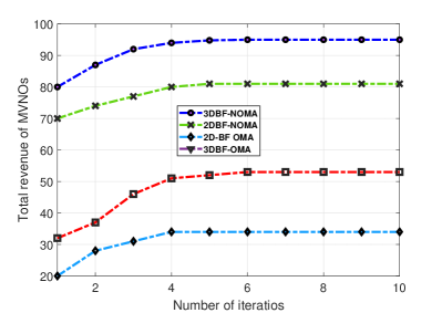
Figure 2: An examples of convergence of SCA algorithm for different network configuration.

IV-B Computational Complexity

In this subsection, we analyze the computational complexity of the proposed solution. The complexity of an iterative algorithm is defined as the total number of iterations that is required to converge the algorithm. Based on our proposed solution, the main computational complexity comes from solving the problem via CVX solver by applying geometric programming and interior point method (IPM) [33], [47]. Based on this method, the overall computation complexity is given by

$$\varpi=\frac{\log\left(\frac{\Omega}{t^{0}\zeta}\right)}{\log(\vartheta)},$$ (35)

where

$$\Omega=7\times F\times K\times N+2\times V+F,$$ (36)

is the total number of constraints of problem (34), $t^{0}$ is the initial point for approximating the accuracy of IPM, $0<\zeta<<1$ is the stopping criterion for IPM and $\vartheta$ is used for updating the accuracy of IPM [48], [49], [31].

V Numerical Results

V-A Simulation Environment

In this section, the system performance of the proposed solution is evaluated under different aspects such as the number of users and FBSs with Monte-Carlo simulations with $300$ iterations. In the numerical results, the system parameters are set as follows:
We assume two different InPs, each of which consists of a single MBS and $4$ FBSs randomly located in the main area with radius $0.5$ km and $20$ m, respectively [50]. Moreover, the bandwidth of each InP is $5$ MHz [51]. The frequency bandwidth of each subcarrier is assumed to be $200$ KHz. Hence, the total number of subcarriers for each InP is $25$. It is also assumed that there are $50$ single-antenna users are randomly distributed in the coverage area of the network at different distances. Moreover, $\Gamma_{f_{i},n_{i},k}^{m}$ is generated according to the complex Gaussian distribution with mean $0$ and variance $1$, i.e., $\bm{\Gamma}_{f_{i},n_{i},k}\thicksim\mathcal{CN}(\mathbb{0}_{M_{T}},\mathbb{I})$, where $\mathbb{I}$ is the identity matrix.

Table II: Configuration of network and setup parameters.

Parameters(s)	Value(s)
$I$	$2$
$V$	$5$
$F_{i}$	$5$
MBS radious, FBS radious	$500$ m, $20$ m
MBS height, FBS height	$32\leavevmode\nobreak\$ m, $2\leavevmode\nobreak\$ m
$P_{\max}^{\text{MBS}}$, $P_{\max}^{\text{FBS}}$	$40$ Wattss, $2\,\text{Watts}$
$\text{BW}_{i}$, $N_{i}$	$5$ MHz, $25$
$K_{\text{Total}}$, $K_{v}$	$50$, $10$
$M_{T}$	$\text{min=5},\text{max}=13$
$L$	$2$
$\hat{\phi}_{3dB}$, $\hat{\theta}_{3dB}$, $\hat{\phi}_{0}$	$65\degree$, $65\degree$, $90\degree$
$\theta_{f_{i},n_{i},k}^{\text{tilt},\min}$, $\theta_{f_{i},n_{i},k}^{\text{tilt},\max}$	$0$, $\pi/2$
$G_{\max,\text{E}}$, $\text{SLL}_{\text{Al}}$, $\text{SLL}_{El}$	$8\leavevmode\nobreak\$ dBi, $30$ dB, $30$ dB
Power spectral density of AWGN noise	$-174$ $\frac{\text{dBm}}{\text{Hz}}$
Channel coeffient	Rayleigh distribution
	with parameter $1$
$\varrho$	$3$

The power spectral density of the received AWGN noise is also set to $-174$ dBm/Hz. Moreover, $G_{\max,\text{E}}$, $\text{SLL}_{\text{Az}}$, and $\text{SLL}_{\text{El}}$ are set to $8$ dBi, $30$ dB, and $30$ dB, respectively [8],[17], [52]. In addition, we set $R_{\min}^{v}=30$ bps/Hz. Furthermore, we assume that $C_{i,f_{i}}=200$, and $G_{v,k}=10^{-6}$. The value of other parameters are summarized in Table II.

V-B Simulation Results

The simulation analyses are provided from two main aspects; 1) The variants of different network parameters, 2) the different solution algorithms; as follows:

V-B1 Various System Parameters

$\bullet\leavevmode\nobreak\ \leavevmode\nobreak\$The Number of Users

Fig. 3 illustrates the total MVNO’s revenue versus the total number of users in the network. It is clear that, 3DBF with NOMA significantly improves the MVNO’s revenue due to increasing achievable data rate of users and system throughput. Moreover, by increasing the number of users, the MVNO’s revenue is increased. That means the MVNO with more customers obtains more revenues in compared to the others with low the number of customers. Hence, not only advanced technologies like multiple antenna BF and NOMA have major effects on the enhancement of system spectral efficiency (throughput), but also it has considerable impact on the revenue of operators and the costs of each InP.
$\bullet\leavevmode\nobreak\ \leavevmode\nobreak\$The Number of FBSs

Fig. 4 shows the total MVNO’s revenue versus the number of FBSs in each InP network by considering the number of users is $35$. Clearly, by increasing the number of BSs, MVNO’s revenue is improved. This is due to each MVNO’s user has better experience and improves the achievable data rate. Hence, users pay more money to their MVNOs. Moreover, in this case probability of reducing path loss is increased and power consumption and its cost are reduced. On the other hand, in this scenario, the system throughout are increased. Hence, the total revenue is directly proportional to the system data rate, also increased.

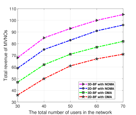
Figure 3: Total Revenue of MVNOs versus the total number of users in networks, with $P_{\max}^{\text{MBS}}=40$ Watts, $P_{\max}^{\text{FBS}}=5$ Watts, $F_{i}=5$, and $M_{T}=5$.

$\bullet\leavevmode\nobreak\ \leavevmode\nobreak\$The Number of Transmit Antennas in Each BS

The effect of number of transmit antenna ($M_{T}$) in each BS is illustrated in Fig. 5. As seen, by increasing the number of transmit antenna in each BS, the total revenue of MVNOs is improved. This is due to the effect of antennas on the system throughput and energy efficiency. More important, in this scenario, 3DBF significantly outperforms 2DBF. As a result, massive antennas with 3DBF system is a key enabler for massive connection networks in case of spectrum is limit or accusation of it has multiple times cost. Moreover, 3DBF reduces inter-cell interference and enhances the system performance from the SE perspective.

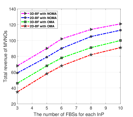
Figure 4: Total Revenue of MVNOs versus the total number of FBs in each InP, with $P_{\max}^{\text{MBS}}=40$ Watts, $P_{\max}^{\text{FBS}}=5$ Watts, $K=50$, and $M_{T}=5$.

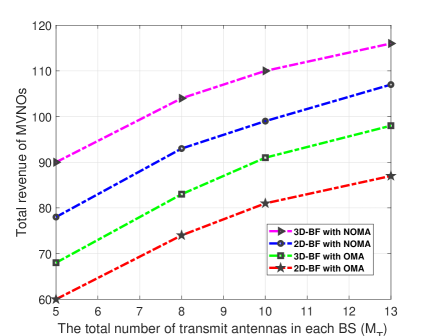
Figure 5: The achieved revenue against the total number of transmit antennas of each BS, with $P_{\max}^{\text{MBS}}=40$ Watts, $P_{\max}^{\text{FBS}}=5$ Watts, $K=50$, and $F=5$.

$\bullet\leavevmode\nobreak\ \leavevmode\nobreak\$The Total Bandwidth of Each InP

In Fig. 6, we investigate the total revenue of MVNOs versus maximum available bandwidth of each BS. Note that in this figure, subcarrier spacing is equal to $200$ KHz. As a result from this analyze, more spectrum for each MVNO makes that it has more revenue. Moreover, in this case NOMA has considerable performance improvement than that of 3DBF. In other words, in case of availability of spectrum, utilizing NOMA has more effects on the revenue compared to enabling 3DBF.

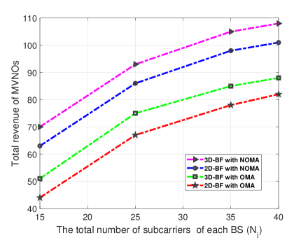
Figure 6: The achieved revenue against the total maximum available bandwidth of each BS, with $P_{\max}^{\text{MBS}}=40$ Watts, $P_{\max}^{\text{FBS}}=5$ Watts, $K=50$, $F=5$, and $M_{T}=5$.

$\bullet\leavevmode\nobreak\ \leavevmode\nobreak\$The Power Budget and Cost Weight

Furthermore, we investigate the maximum allowable power of MBSs impact on the total revenue of MVNOs with different cost weights, i.e., $C_{i,f_{i}}$ in Fig. 7. This figure depicts the comparison between different cost weights for power consumption in the InPs network. As a result from this figure, with NOMA and 3DBF the total revenue of MVNOs improve up with approximately $54$% compared to 2DBF with OMA. This is because, not only utilizing NOMA allows that each resource block, i.e., subcarrier can be exploited more than one times without imposing inter-cell interference, but also 3DBF massive antenna systems has a major improvement on the sum rate of users without more power consumption. Hence, based on the high income of MVNOs and the cost reduction of power consumption, the total revenue of MVNOs increases. Moreover, Fig. 7 highlights that high cost weights for power consumption decreases the total revenue of MVNOs in contrast to power budget enhancement.

We emphasize the performance and complexity comparison of the considered techniques in Table VI, based on the parameters shown in Fig. 3 as an example of configuration. As seen, exploiting 3DBF and NOMA improves the total revenue by approximately $47$% compared to 2DBF with OMA. This is because of, in 3DBF NOMA network, the SINR of each user is improved by adjusting the the beam pattern of antennas as desired and with NOMA the system throughput is increased. On the other hand, our proposed revenue is based on the received data rate of users. Hence, these results are observed.
$\bullet\leavevmode\nobreak\ \leavevmode\nobreak\$Deployment Scenarios

Based on the 3-rd generation partnership project (3GPP) standardization, from geographical locations perspective, we have $4$ main areas as deployment scenarios that are presented in Table IV [53], [54], [37]. Based on this, we to evaluate the proposed problem in these scenarios to verify its practicality. In this regard, we configure the network according to the characteristics of these scenarios, in which the considered system parameters are depicted in Table V for a small scaled network. Table III compares the performance of 2DBF and 3DBF for different access technologies and various deployment scenarios in Table IV. In this Table, we consider 2DBF with OMA access is baseline and comparison values are listed with defined ratio as $\frac{\text{Mentioned technology name}}{\text{2DBF OMA}}$, as an example $\frac{\text{3DBF NOMA}}{\text{2DBF OMA}}$. From this results, we obtain that 3DBF with NOMA is the most beneficial option for Indoor hotspot locations. This is has two main reasons, the first is the efficiency of NOMA, since the number of users is high and SE of NOMA is more than that of the other scenarios. The second is refereed to the performance of 3DBF in which it improves the received SINR of users by assigning pencil beams with high gains to them. Moreover, in these scenarios, the data rate of users that are located in different floors and blind locations are significantly improved.

Table III: Performance comparison of different technologies in different geographical locations (deployment scenarios) based on the setting in Table V.

Technologies
		2DBF with NOMA	3DBF with OMA	3DBF with NOMA
Scenarios	Indoor hotspot	2.7x	2.3x	4.6x
	Dense urban	2.3x	1.9x	3.8x
	Urban	1.7x	1.6x	3.2x
	Suburban/Rural	1.3x	1.4x	2.1x

$\bullet\leavevmode\nobreak\ \leavevmode\nobreak\$Signaling overhead of 2D and 3D channels

Radio resource management in NR is based on the measurement of reference signals such as synchronization and channel information, i.e., CSI [55]. Some of them are used for time and frequency synchronization in the random access procedure and demodulation of signals at receiver sides (via demodulation reference signal). In this paper, signaling overhead refers to the amount of feedback required for the 2D and 3D channels estimation. In the 3D channel, channel information is required for both horizontal and vertical directions, in contrast to the 2D channel model that is just in the horizontal direction. As a result, the predefined overhead signal is increased rapidly in 3D by the number of antennas and the BSs in the network. We compare the 2D and 3D channels with signaling overhead metric in Table VII, where, assuming the number of vertical antennas is $M_{T}^{\prime}$. We infer that the ratio of signaling overhead of 3DBF over 2DBF is closed together in high order of transmit antennas.

Table IV: Assumptions and main characteristics for deriving different deployment scenarios for 5G based on the 3GPP specifications.

	Overall User density ($\text{per}{\text{Km}}^{2}$)	Active user data rate (Mbps)	Activity factor
Indoor	$250000$	$200$	$30\%$
Dense Urban	25000	300	$10\%$
Urban	10000	50	$20\%$
Rural	100	50	$20\%$

Table V: Network configuration in different deployment scenarios, other parameters are based on Table II.

Deployment scenario
		Indoor	Dense urban	Urban	Suburban/ Rural
Network Configuration	BS Height	15 m	25 m	35 m	45 m
	Maximum transmit power	10 Watts	20 Watts	40 Watts	60 Watts
	The number of carriers	100	64	40	20
	Inter-site distance	20 m	200 m	500 m	5000 m
	Number of antennas ($M_{T}$)	15	12	8	5
	User Density	200/$\text{km}^{2}$	150/$\text{km}^{2}$	70/$\text{km}^{2}$	30/$\text{km}^{2}$

Table VI: Complexity order and performance comparison of 2DBF with OMA and 3DBF with NOMA according to Fig. 3.

Metric	2DBF OMA	3DBF NOMA	3D-NOMA over 2D-OMA
Complexity	$\mathcal{O}\left(2V+F+F\times N\times K\right)$	$\mathcal{O}\left(2V+F+4\times F\times N\times K+F\times N\right)$	$0.75\%\uparrow$
Objective	71	105	$47\%\uparrow$

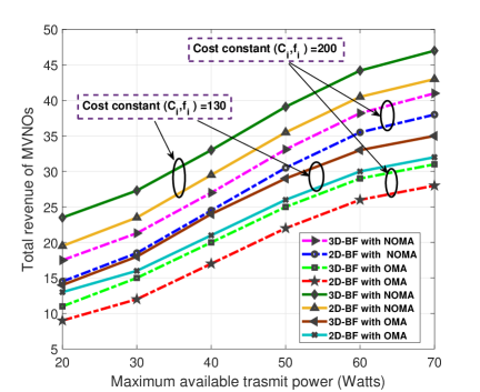
Figure 7: The total Revenue of MVNOs versus the maximum transmit power budget, with $U=30$ Watts, $N_{i}=25$, $F_{i}=5$ and $M_{T}=5$.

Table VII: Signaling overhead comparison of the 2DBF and 3DBF.

Metric	2DBF	3DBF	3DBF over 2DBF
Overhead	$M_{T}\times F=13\times 10=130$	$(M_{T}+M_{T}^{\prime})\times F=(13+2)\times 10=150$	$15\%\uparrow$

V-B2 Comparison Between the Proposed Solution Methods

In this subsection, we investigate different solutions, namely, JS-CIV, ASM, and optimal in which each of them is briefly discussed in the following.
$\bullet\leavevmode\nobreak\ \leavevmode\nobreak\$JS-CIV

We propose JS-CIV to solve problem (34). To this end, we convert non-convex main problem (20) to convex problem (34). The main step is to convert the binary variable, i.e., $\bm{\rho}$ to the predefined optimization variable, i.e., $\mathbb{W}$. Then, by exploiting the change variable method and first Taylor approximation, we formulate problem (34). Finally, we solve it with SCA (Al. 1). Note that in this method, we solve all considered optimization variables jointly.
$\bullet\leavevmode\nobreak\ \leavevmode\nobreak\$ASM

Based on the ASM method, we divide main problem (20) into two sub-problems, namely, joint subcarrier and user association and 3D beam allocation. Then, we solve each on them separately and iterate between them until stopping criteria are met. Note that in this method, we also use SCA-based difference of concave functions and first order of Taylor approximation in the 3D beam allocation sub-problem.
$\bullet\leavevmode\nobreak\ \leavevmode\nobreak\$Optimal

We devise the exhaustive search method to investigate the optimality gap of the iterative sub-optimal solutions in the considered parameters. Fig. 8 illustrates the performance comparison of the aforementioned solutions. As seen, the optimality gap of the proposed solution, i.e., JS-CIV is nearly $8$%, while this gap is $15$% for ASM. This is because of disjoint solving of the integer and continues variables in ASM, in contrast to jointly solving of them with SCA. Moreover, we compare the complexity order of the mentioned solutions that is stated in Table VIII. In this table, $\Omega$ is obtained from (36), $E^{\text{Pos}}$, and $Q^{\text{Pos}}$ are different possible values in the exhaustive search method for $\mathbb{W}$ and $\bm{\theta}$, respectively.

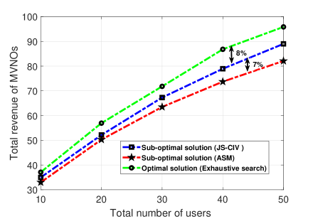
Figure 8: Total Revenue of MVNOs versus the total number of users in networks, with $P_{\max}^{\text{MBS}}=30$ Watts, $P_{\max}^{\text{FBS}}=5$ Watts, $F_{i}=4$ and $M_{T}=5$ for different solutions methods.

Table VIII: Complexity order and performance comparison of the proposed solutions according to Table II and Fig. 8.

	JS-CIV	ASM	Optimal
Complexity	$\varpi=\frac{\log\left(\frac{\Omega}{t^{0}\zeta}\right)}{\log(\vartheta)}$	$\frac{\log\left(\frac{2(V+F\times N\times K)+N\times F\times I}{t^{0}\zeta}\right)}{\log(\vartheta)}+\frac{\log\left(\frac{2V+F\times N(1+K)+F\times I}{t^{0}\zeta}\right)}{\log(\vartheta)}$	$(2E^{\text{Pos}})^{(U\times N)}\times(Q^{\text{Pos}})^{(U\times M\times F\times I)}$
Performance	$8\%\downarrow$	$15\%\downarrow$	Baseline

VI conclusion

In this paper, we studied a novel multi-user MISO-3DBF-NOMA-based HetNet from the cost and the system performance perspectives. Our proposed optimization problem is based on the maximizing MVNO’s total revenue under resource limitation and guaranteeing the user’s required QoS and contains both integer and continues variables. To solve the proposed optimization problem efficiently, we propose a new algorithm called JS-CIV where it solves the main problem without adopting ASM, by exploiting the change variables method. Our evaluations, benchmarked against a baseline, demonstrated that the impact of utilizing 3DBF in NOMA-based HetNet from the performance and MVNO’s revenue perspectives. Furthermore, the convergence of the proposed algorithm is verified in our evaluations. Our numerical results show that 3DBF has good performance in massive antennas systems. Also NOMA is very appropriate for ultra high density environments which require very high spectrum. Indeed, NOMA-3DBF significantly improves the system throughput and subsequently the MVNO’s revenue can be improved with approximately $54$% in massive connection networks. Moreover, we investigated the proposed system model for different deployment scenarios and signaling overhead as a metric. Moreover, JS-CIV outperforms ASM and its optimality gap is nearly $8$%. As a future work, we aim to study the proposed algorithm for imperfect CSI.

References

- [1] Z. Lin, M. Lin, J. Wang, T. De Cola, and J. Wang, “Joint beamforming and power allocation for satellite-terrestrial integrated networks with non-orthogonal multiple access,” IEEE Journal of Selected Topics in Signal Processing, pp. 1–1, 2019.
- [2] Z. Ding, X. Lei, G. K. Karagiannidis, R. Schober, J. Yuan, and V. K. Bhargava, “A survey on non-orthogonal multiple access for 5G networks: Research challenges and future trends,” IEEE Journal on Selected Areas in Communications, vol. 35, no. 10, pp. 2181–2195, 2017.
- [3] M. Agiwal, A. Roy, and N. Saxena, “Next generation 5G wireless networks: A comprehensive survey,” IEEE Communications Surveys Tutorials, vol. 18, pp. 1617–1655, thirdquarter 2016.
- [4] H. Al-Obiedollah, K. Cumanan, J. Thiyagalingam, A. G. Burr, Z. Ding, and O. A. Dobre, “Sum rate fairness trade-off-based resource allocation technique for MISO NOMA systems,” arXiv preprint arXiv:1902.05735, 2019.
- [5] “5G spectrum public policy position,” Huawei Technologies Co. Ltd. Dec. 2017.
- [6] “5G NR: A new era for enhanced mobile broadband,” MediaTek, Inc. Apr. 2018.
- [7] T. S. El-Bawab, R. Subrahmanyan, G. Atkin, and M. Dohler, “Key technology for 5G new radio,” IEEE Communications Magazine, p. 2, 2018.
- [8] Q.-U.-A. Nadeem, A. Kammoun, and M.-S. Alouini, “Elevation beamforming with Full dimension MIMO architectures in 5G systems: A tutorial,” arXiv preprint arXiv:1805.00225, 2018.
- [9] L. Dai, B. Wang, Y. Yuan, S. Han, C. I, and Z. Wang, “Non-orthogonal multiple access for 5G: solutions, challenges, opportunities, and future research trends,” IEEE Communications Magazine, vol. 53, pp. 74–81, Sep. 2015.
- [10] Y. Jeong, C. Lee, and Y. H. Kim, “Power minimizing beamforming and power allocation for MISO-NOMA systems,” IEEE Transactions on Vehicular Technology, pp. 1–1, 2019.
- [11] X. Sun, N. Yang, S. Yan, Z. Ding, D. W. K. Ng, C. Shen, and Z. Zhong, “Joint beamforming and power allocation in downlink NOMA multiuser MIMO networks,” IEEE Transactions on Wireless Communications, vol. 17, pp. 5367–5381, Aug. 2018.
- [12] M. Vaezi, G. Amarasuriya, Y. Liu, A. Arafa, F. Fang, and Z. Ding, “Interplay between NOMA and other emerging technologies: A survey,” arXiv preprint arXiv:1903.10489, 2019.
- [13] A. Zakeri, M. Moltafet, and N. Mokari, “Joint radio resource allocation and SIC ordering in NOMA-based networks using submodularity and matching theory,” IEEE Transactions on Vehicular Technology, pp. 1–1, 2019.
- [14] Z. Xiao, L. Zhu, J. Choi, P. Xia, and X.-G. Xia, “Joint power allocation and beamforming for non-orthogonal multiple access (NOMA) in 5G millimeter-wave communications,” IEEE Transactions on Wireless Communications, vol. 17, no. 5, pp. 2961–2974, 2018.
- [15] Y. Li, X. Ji, M. Peng, Y. Li, and C. Huang, “An enhanced beamforming algorithm for three dimensional MIMO in LTE-advanced networks,” in Wireless Communications & Signal Processing (WCSP), 2013 International Conference on, pp. 1–5, 2013.
- [16] H. Al-Obiedollah, K. Cumanan, J. Thiyagalingam, A. G. Burr, Z. Ding, and O. A. Dobre, “Energy efficient beamforming design for MISO non-orthogonal multiple access systems,” IEEE Transactions on Communications, pp. 1–1, Feb. 2019.
- [17] A. Kammoun, M. Debbah, M.-S. Alouini, et al., “Design of 5G full dimension massive MIMO systems,” IEEE Transactions on Communications, vol. 66, no. 2, pp. 726–740, 2018.
- [18] R. Shafin, L. Liu, and J. C. Zhang, “On the channel estimation for 3D massive MIMO systems,” E-LETTER, 2014.
- [19] J. Cui, Y. Liu, Z. Ding, P. Fan, and A. Nallanathan, “Optimal user scheduling and power allocation for millimeter wave noma systems,” IEEE Transactions on Wireless Communications, vol. 17, no. 3, pp. 1502–1517, 2018.
- [20] H. Utatsu, K. Osawa, J. Mashino, S. Suyama, and H. Otsuka, “Throughput performance of relay backhaul enhancement using 3D beamforming,” in Proc. (ICOIN), Kuala Lumpur, Malaysia, PP. 120-124, Jan. 2019.
- [21] W. Shin, M. Vaezi, B. Lee, D. J. Love, J. Lee, and H. V. Poor, “Coordinated beamforming for multi-cell MIMO-NOMA,” IEEE Communications Letters, vol. 21, pp. 84–87, Jan. 2017.
- [22] Y. Li, X. Ji, D. Liang, and Y. Li, “Dynamic beamforming for three-dimensional MIMO technique in lte-advanced networks,” International journal of antennas and propagation, p. 8, Jul 2013.
- [23] O. Alluhaibi, M. Nair, A. Hazzaa, A. Mihbarey, and J. Wang, “3D beamforming for 5G millimeter wave systems using singular value decomposition and particle swarm optimization approaches,” in 2018 International Conference on Information and Communication Technology Convergence (ICTC), pp. 15–19, Oct 2018.
- [24] K. Xiao, L. Gong, and M. Kadoch, “Opportunistic multicast NOMA with security concerns in a 5G massive MIMO system,” IEEE Communications Magazine, vol. 56, no. 3, pp. 91–95, 2018.
- [25] Z. Wang, W. Liu, C. Qian, S. Chen, and L. Hanzo, “Two-dimensional precoding for 3-D massive MIMO,” IEEE Transactions on Vehicular Technology, vol. 66, pp. 5485–5490, June 2017.
- [26] Y. Chi, L. Liu, G. Song, C. Yuen, Y. L. Guan, and Y. Li, “Practical MIMO-NOMA: Low complexity and capacity-approaching solution,” IEEE Transactions on Wireless Communications, vol. 17, no. 9, pp. 6251–6264, 2018.
- [27] J. Cui, Z. Ding, and P. Fan, “Outage probability constrained MIMO-NOMA designs under imperfect CSI,” IEEE Transactions on Wireless Communications, vol. 17, pp. 8239–8255, Dec 2018.
- [28] H. Al-Obiedollah, K. Cumanan, J. Thiyagalingam, A. G. Burr, Z. Ding, and O. A. Dobre, “Energy efficiency fairness beamforming designs for MISO NOMA systems,” arXiv preprint arXiv:1902.05732, 2019.
- [29] M. Alhusseini, P. Azmi, and N. Mokari, “Optimal joint subcarrier and power allocation for MISO-NOMA satellite networks,” Physical Communication, vol. 32, pp. 50–61, Nov. 2019.
- [30] A. Rezaei, P. Azmi, N. Mokari, and M. R. Javan, “Robust resource allocation for PD-NOMA-based MISO heterogeneous networks with CoMP technology,” arXiv preprint arXiv:1902.09879, 2019.
- [31] M. Moltafet, S. Parsaeefard, M. R. Javan, and N. Mokari, “Robust radio resource allocation in MISO-SCMA assisted C-RAN in 5G networks,” IEEE Transactions on Vehicular Technology, vol. 68, pp. 5758–5768, Jun 2019.
- [32] H. Al-Obiedollah, K. Cumanan, J. Thiyagalingam, A. G. Burr, Z. Ding, and O. A. Dobre, “Energy efficient beamforming design for MISO non-orthogonal multiple access systems,” IEEE Transactions on Communications, 2019.
- [33] F. Alavi, K. Cumanan, Z. Ding, and A. G. Burr, “Robust beamforming techniques for non-orthogonal multiple access systems with bounded channel uncertainties,” IEEE Communications Letters, vol. 21, no. 9, pp. 2033–2036, 2017.
- [34] X. Li, L. Li, F. Wen, J. Wang, and C. Deng, “Sum rate analysis of MU-MIMO with a 3D MIMO base station exploiting elevation features,” International Journal of Antennas and Propagation, vol. 2015, 2015.
- [35] L. Fan, H. Zhang, Y. Huang, and L. Yang, “Exploiting bs antenna tilt for swipt in 3-D massive MIMO systems,” IEEE Wireless Communications Letters, vol. 6, no. 5, pp. 666–669, 2017.
- [36] M. Baianifar, S. M. Razavizadeh, H. Akhlaghpasand, and I. Lee, “Energy efficiency maximization in mmwave wireless networks with 3D beamforming,” Journal of Communications and Networks, vol. 21, pp. 125–135, April 2019.
- [37] “Technical performance requirements for IMT-2020,” ITU Radiocommunication Study Groups. Jun. 2016.
- [38] F. Fang, H. Zhang, J. Cheng, S. Roy, and V. C. M. Leung, “Joint user scheduling and power allocation optimization for energy-efficient NOMA systems with imperfect CSI,” IEEE Journal on Selected Areas in Communications, vol. 35, pp. 2874–2885, Dec 2017.
- [39] X. Foukas, G. Patounas, A. Elmokashfi, and M. K. Marina, “Network slicing in 5G: Survey and challenges,” IEEE Communications Magazine, vol. 55, pp. 94–100, May 2017.
- [40] Y.-H. Nam, M. S. Rahman, Y. Li, G. Xu, E. Onggosanusi, J. Zhang, and J.-Y. Seol, “Full dimension MIMO for LTE-advanced and 5G,” in 2015 Information Theory and Applications Workshop (ITA), pp. 143–148, IEEE, 2015.
- [41] M. Moltafet, N. Mokari, M. R. Javan, H. Saeedi, and H. Pishro-Nik, “A new multiple access technique for 5G: Power domain sparse code multiple access (PSMA),” IEEE Access, vol. 6, pp. 747–759, Nov. 2018.
- [42] Y. Sun, D. W. K. Ng, Z. Ding, and R. Schober, “Optimal joint power and subcarrier allocation for full-duplex multicarrier non-orthogonal multiple access systems,” IEEE Transactions on Communications, vol. 65, pp. 1077–1091, Mar. 2017.
- [43] ““study on downlink multiuser supersition transmission (MUST) for LTE (release 13),” 3GPP TR 36.859, tech. rep., dec. 2015,”
- [44] Z. Ding, P. Fan, and H. V. Poor, “Impact of user pairing on 5G nonorthogonal multiple-access downlink transmissions,” IEEE Transactions on Vehicular Technology, vol. 65, pp. 6010–6023, Aug. 2016.
- [45] Y. Liu, Z. Ding, M. Eïkashlan, and H. V. Poor, “Cooperative non-orthogonal multiple access in 5G systems with SWIPT,” in Proc. EUSIPCO, Nice, France, Aug. 2015, pp 1999-2003.
- [46] T. Lv, H. Gao, and S. Yang, “Secrecy transmit beamforming for heterogeneous networks,” IEEE Journal on Selected Areas in Communications, vol. 33, pp. 1154–1170, Jun. 2015.
- [47] N. Mokari, F. Alavi, S. Parsaeefard, and T. Le-Ngoc, “Limited-feedback resource allocation in heterogeneous cellular networks,” IEEE Transactions on Vehicular Technology, vol. 65, no. 4, pp. 2509–2521, 2016.
- [48] S. Boyd and L. Vandenberghe, Convex optimization. Cambridge university press, 2004.
- [49] M. Grant, S. Boyd, and Y. Ye, “CVX: Matlab software for disciplined convex programming,” 2008.
- [50] D. T. Ngo, S. Khakurel, and T. Le-Ngoc, “Joint subchannel assignment and power allocation for OFDMA femtocell networks,” IEEE Transactions on Wireless Communications, vol. 13, pp. 342–355, Jan. 2014.
- [51] T. E. Bogale and L. B. Le, “Massive MIMO and mmwave for 5G wireless hetnet: Potential benefits and challenges,” IEEE Vehicular Technology Magazine, vol. 11, pp. 64–75, Mar. 2016.
- [52] A. Kammoun, H. Khanfir, Z. Altman, M. Debbah, and M. Kamoun, “Preliminary results on 3D channel modeling: From theory to standardization,” IEEE Journal on Selected Areas in Communications, vol. 32, no. 6, pp. 1219–1229, 2014.
- [53] “3GPP TS 22.261 technical specification group services and system aspects; service requirements for the 5G system; stage 1(release 16),”
- [54] “Recommendations for NGMN KPIs and requirements for 5G,” NGMN Alliance. Jun. 2016.
- [55] B. Bertenyi, S. Nagata, H. Kooropaty, X. Zhou, W. Chen, Y. Kim, X. Dai, and X. Xu, “5G NR radio interface,” Journal of ICT Standardization, vol. 6, no. 1, pp. 31–58, 2018.