High-Harmonic Generation in a Correlated Electron System

Abstract

High-harmonic generation (HHG) in crystalline solids have been examined so far on the basis of one-body energy-band structures arising from electron itineracy in a periodic potential. Here, we show emergence of HHG signals which are attributed to dynamics of many-body states in a low-dimensional correlated electron system. An interacting fermion model and its effective pseudo-spin model on a one-dimensional dimer-type lattice are analyzed. Observed HHG signals in a spontaneously symmetry-broken state, where charge densities are polarized inside of dimer units, show threshold behavior with respect to light amplitude and are interpreted in terms of tunneling and recombination of kink-antikink excitations in an electric field.

Photoinduced nonequilibrium electron dynamics in solids have attracted much attention of researchers not only in condensed matter physics but also in optical physics. Recent great progress in intense laser pulse, ultrafast time-resolved experimental probes, and theoretical methods for nonequilibrium systems has opened up a new research field of exotic light-induced phenomena. High-order harmonic generation (HHG) is one of the attractive phenomena induced by intense laser light huttner ; kruchinin ; ghimire2 . This is a nonlinear and nonperturbative light-matter coupled phenomenon, and is widely recognized to be utilized to generate the attosecond X-ray laser pulse. Studies of HHG have been developed in atom- and molecule-gas systems agostini ; krausz ; gallmann ; corkum ; lewenstein ; ishikawa , in which the HHG spectra consist of a characteristic plateau and cut-off energy. This behavior is well explained by the three-step model, i.e., a sequential process of ionization, forced oscillatory motion, and recombination of electrons in atomic/molecular potentials corkum ; lewenstein . In crystalline solids where the atom are aligned periodically, electronic processes involved in HHG are considered on the basis of the Bloch energy bands due to electron itineracy huttner ; kruchinin ; ghimire2 ; ghimire ; hohenleutner ; liu ; yoshikawa ; ndabashimiye ; higuchi ; hawkins ; vampa ; mcdonald ; wu2 ; hansen ; ikemachi ; ikemachi2 ; ikeda ; kruchinin2 . An extended three-step model based on the band structure was proposed to explain the characteristic plateau in HHG observed in several crystalline solids wu2 ; ikemachi ; hansen .

Beyond conventional semiconductors and metals, to which the one-body Bloch-band picture is applicable, correlated electron systems have great potentialities of HHG. Large energy scale and fast dephasing due to strong electron-electron interactions ishikawa ; liu ; ikemachi2 ; kruchinin2 and existence of multiple ordered phases are supposed to be great advantages for HHG. One example is that a large third-harmonic generation in a perturbative regime which is observed in one-dimensional copper oxides is attributed to an electron-electron interaction effect kishida ; ogasawara . In recent years, HHG has started to be examined in correlated electron systems from a viewpoint of quasi-particle motion silva ; murakami ; dejean ; takayoshi ; zhu .

In this Letter, we show that HHG spectra emerge owing to many-electron dynamics in a correlated electron system, rather than the Bloch electron itineracy. We analyze photoinduced dynamics of an interacting fermion model on a dimer-type lattice and its low-energy effective model described by the pseudo-spin (PS) operators. We find emergence of HHG spectra in a spontaneously symmetry-broken state, in which charge densities are polarized inside of dimer units. The HHG spectra show a threshold behavior with respect to light amplitude. As shown in Fig. 1(c), the observed HHG are explained by an extended three-step like processes for many-body kink-antikink excitations, which are valid even without electron itineracy.

A target system of the present study is an interacting electron system with a one-dimensional dimer-type lattice structure shown in Fig. 1(a). It is well known that when the average number of electrons is 0.5 per site under a strong on-site electron interaction, there are two competing electronic states in the ground state (GS): a Mott insulating state where the bonding-orbital band is half filled, termed the dimer Mott (DM) insulating state, and the polar charge-ordered (CO) state where electron distribution inside the each dimer unit breaks the inversion symmetry [see Fig. 1(c)] kino ; naka ; hotta . We analyze the two model Hamiltonians introduced below MM . An interacting spinless-fermion model in a dimer lattice is defined as

$${\cal H}_{\rm SF} =-\sum_{i}\left(t_{0}f_{ia}^{\dagger}f_{ib}+{\rm H.c.}\right)-\sum_{i}\left(t^{\prime}f_{ib}^{\dagger}f_{i+1a}+{\rm H.c.}\right)$$

$$\quad+V_{0}\sum_{i}n_{ia}n_{ib}+V^{\prime}\sum_{i}n_{ib}n_{i+1a},$$ (1)

where $f_{i\gamma}^{\dagger}$ ($f_{i\gamma}$) is the creation (annihilation) operator of a spinless fermion at the $i$th unit cell and sublattice $\gamma\ (=a,b)$, and $n_{i\gamma}=f_{i\gamma}^{\dagger}f_{i\gamma}$ is the number operator. The first two terms represent the fermion hoppings, and the last two terms describe the inter-site Coulomb interactions. The total number of the fermions is set to $N$ with $N$ being the total number of the dimer units. We analyze another Hamiltonian for an interacting PS system as a low-energy effective model of ${\cal H}_{\rm SF}$ naka ; tsuchiizu . The local electronic states inside the dimer unit are described by the PS operator: the up and down PSs imply the states where electron occupies the $a$ (left) and $b$ (right) sites in the dimer unit, respectively. The low-energy physics is mapped onto the transverse Ising (TI) model defined by

$${\cal H}_{\rm TI}=-\frac{V^{\prime}}{4}\sum_{\langle ij\rangle}{\sigma}_{i}^{z}{\sigma}_{j}^{z}-t_{0}\sum_{i}\sigma_{i}^{x},$$ (2)

where ${\bm{\sigma}}_{i}$ are the Pauli matrices located at the $i$th unit cell. The first term (${\cal H}_{I}$) and the second term (${\cal H}_{T}$) describe the interaction between the nearest neighbor unit cells, and the transverse field, respectively. These terms correspond to the inter-dimer Coulomb interaction and the intra-dimer hopping in Eq. (1), respectively. This model is suitable to study the collective excitations, i.e., the kink and antikink (domain-wall) excitations.

A vector potential of light is introduced as the Peierls phase as $t_{0}\rightarrow t_{0}e^{-iA(t)}$ and $t^{\prime}\rightarrow t^{\prime}e^{-iA(t)}$ in Eq. (1), where $A(t)$ is the vector potential at time $t$ and the difference in the bond lengths are neglected. The electric field is given by $E(t)=-\partial A(t)/\partial t$. This coupling corresponds to the rotation of the transverse field as follows MM : ${\cal H}_{T}$ is replaced by $-t_{0}\sum_{i}\left[\cos A(t)\,\sigma_{i}^{x}-\sin A(t)\,\sigma_{i}^{y}\right]$, and the electric current operator is identified as $\hat{j}(t)=-(t_{0}/N)\sum_{i}\left[\sin A(t)\,\sigma_{i}^{x}+\cos A(t)\,\sigma_{i}^{y}\right]$. We confirmed that the numerical results of HHG in the above two models qualitatively coincide in the polar CO state, and we will mainly present the results for the TI model.

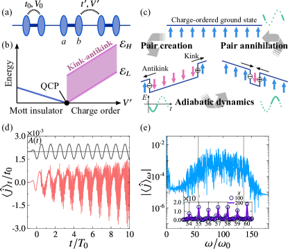
Figure 1: (a) A schematic dimer-type lattice and interactions. The ovals and the thick bars represent atoms and dimer bonds, respectively. (b) Schematic kink-antikink excitation spectra in the TI model. A shaded area represents the kink-antikink band in the CO state. The quantum-critical point (QCP) is indicated as the dot. (c) Sketches of the PS configurations, the kink-antikink pair, and the present HHG process. (d) Time profiles of vector potential $A(t)$ and current $\langle\hat{j}\rangle_{t}$. (e) Fourier transform of the current $\langle\hat{j}\rangle_{\omega}$. The vertical lines indicate ${\cal E}_{H}$ and ${\cal E}_{L}$. Inset shows an enlargement. The iTEBD method is utilized in (d) and (e). Inset of (e) shows the results with $\chi=100$ and 200. We set $V^{\prime}/(4t_{0})=2.4$, $A_{0}=5.8$, $\omega_{0}/t_{0}=0.1$, and $\tau=1/\omega_{0}$.

The GS and excited states in the TI model without the light field have been settled kirilyuk . The GS is the DM insulating state (a paramagnetic PS state), i.e., $\langle\sigma^{z}\rangle=0$ for $V^{\prime}/(4t_{0})<1$, and is the polar CO state (a ferromagnetic PS state) with spontaneous symmetry breaking of the space-inversion symmetry, i.e., $\langle\sigma^{z}\rangle\neq 0$ for $V^{\prime}/(4t_{0})>1$. The boundary at $V^{\prime}/(4t_{0})=1$ is the quantum critical point. In order to calculate the transient dynamics induced by the light field in the thermodynamic limit, the infinite time-evolving block decimation (iTEBD) method is adopted vidal . The second-order Suzuki-Trotter decomposition is utilized to calculate the time-evolution of the wavefunction $|\psi(t+\delta t)\rangle\approx e^{-i{{\cal H}(t)}\delta t}|\psi(t)\rangle$ with a small time difference $\delta t$ and the time-dependent Hamiltonian ${\cal H}(t)$. In most of the numerical calculations, the maximum number of the matrix dimension ($\chi$) in the iTEBD method, and the time difference are chosen to $\chi=200$ and $\delta t=0.01/t_{0}$, respectively, which are enough to obtain well convergent results as shown later [see inset of Fig. 1(e)]. We also adopt the exact diagonalization (ED) method based on the Lanczos algorithm for finite size clusters, where the total number of dimer units is $N=16$ and $18$ with the periodic-boundary condition. The optical absorption spectra [see Fig. S.4 in the Supplemental Material (SM)] is schematically depicted in Fig. 1(b). In the polar CO state, the excitation spectra are attributed to the kink-antikink pair excitations, and exhibit a continuous band where the upper and lower edges of the band are ${\cal E}_{H}=4(V^{\prime}/4+t_{0})$ and ${\cal E}_{L}=4(V^{\prime}/4-t_{0})$, respectively. In the DM state, the low-energy collective excitation is located at $2(t_{0}-V^{\prime}/4)$.

First, we show the HHG spectra in the polar CO state [$V^{\prime}/(4t_{0})=2.4$] in the continuous-wave (cw) light. We set $A(t)=-A_{0}e^{-t^{2}/(2\tau^{2})}\cos(\omega_{0}t)$ for $t<0$, and $A(t)=-A_{0}\cos(\omega_{0}t)$ for $t>0$ with frequency $\omega_{0}$, amplitude $A_{0}$, and raising time $\tau$. Numerical values of $\omega_{0}$ are chosen to be much smaller than the excitation energy gap $\Delta_{\rm gap}={\cal E}_{L}$. Time profiles of the electric current $\langle\hat{j}\rangle_{t}$ and its Fourier transform $\langle\hat{j}\rangle_{\omega}$, as well as $A(t)$, are shown in Figs. 1(d) and 1(e). A multiple pulse-like profile with period of $T_{0}\equiv 2\pi/\omega_{0}$ appears in $\langle\hat{j}\rangle_{t}$, and a series of sharp spikes at $\omega=n\omega_{0}$ with integer number $n$ appear in $\langle\hat{j}\rangle_{\omega}$ [see inset of Fig. 1(e)]. The HHG spectra show a plateau approximately between ${\cal E}_{L}$ and ${\cal E}_{H}$, indicating the nonperturbative processes for this HHG. Owing to the breaking of the space-inversion symmetry in the GS, both the odd and even orders of high harmonics emerge. Overall features mentioned above do not depend on $\chi(\geq 100)$ and are almost reproduced by the ED method in finite-size clusters as shown in Fig. S.2 in SM.

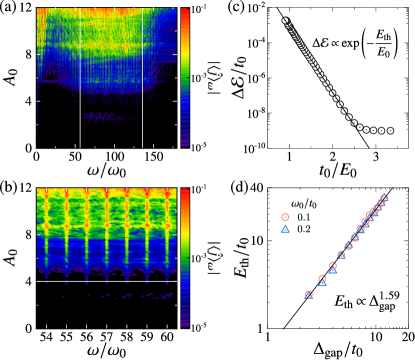
Figure 2: (a) Intensity maps of $\langle\hat{j}\rangle_{\omega}$. The vertical lines show the lower and upper edges of the kink-antikink band. (b) An enlargement of (a). The horizontal line indicates threshold intensity. (c) A logarithmic plot of the absorbed energy $\Delta{\cal E}$ as a function of inverse of $E_{0}$. The bold line shows $\Delta{\cal E}\propto\exp(-E_{\rm th}/E_{0})$. (d) A threshold electric field $E_{\rm th}$ as a function of the gap energy $\Delta_{\rm gap}$. The bold line shows $E_{\rm th}\propto\Delta_{\rm gap}^{\alpha}$ with $\alpha\sim 1.59$. The cw and one-cycle pulse field are introduced in (a) and (b), and (c) and (d), respectively. We set $V^{\prime}/(4t_{0})=2.4$, $\omega_{0}/t_{0}=0.1$, and $\tau=1/\omega_{0}$. The iTEBD method is utilized.

The HHG spectra are sensitive to the light amplitude $A_{0}$. In Figs. 2(a) and 2(b), the intensity map of $\langle\hat{j}\rangle_{\omega}$ in the $\omega$-$A_{0}$ plane and its enlargement are shown, respectively. The threshold behavior of the HHG spectra with respect to $A_{0}$ is clearly seen. We find that the threshold decreases with decreasing $V^{\prime}$ (see Fig. S.1 in SM).

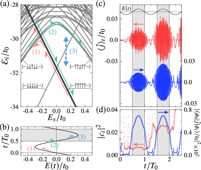
Figure 3: Results based on the adiabatic kink-antikink dynamics. (a) Energy level diagram as a function of $E_{s}$. The bold line represents the energy of the state $|\phi_{0}(E_{s})\rangle$ adiabatically connected to the all-up state at $E_{s}=0$. (b) A schematic time profile of $E(t)$. (c) Time profiles of $E(t)$ (black line) and $\langle\hat{j}\rangle_{t}$ (red line) induced by the cw light. The blue line shows the results calculated from the energy level diagram in (a) (see text). (d) Time profiles of the population of the most dominant excited state $|c_{i}|^{2}$ (red circles), and a square of the transition amplitude $|\langle\phi_{0}(E_{s})|\hat{j}|\phi_{i}(E_{s}\rangle|^{2}$ (blue triangles). Shaded areas in (b)-(d) represent time domains where $E(t)$ is positive. We set $V^{\prime}/(4t_{0})=1.6$, $A_{0}=3.6$, $\omega_{0}/t_{0}=0.1$, $\tau=1/\omega_{0}$, and $N=18$.

The observed HHG is understood by repetition of dynamics induced by a one-cycle pulse. Thus, to reveal the threshold behavior in more detail, we examine responses to a one-cycle pulse given by $A(t)=-A_{0}e^{-t^{2}/(2\tau^{2})}\cos(\omega_{0}t)$. Using the iTEBD method, we analyze the absorbed energy defined by $\Delta{\cal E}\equiv{\cal E}(t\gg\tau)-{\cal E}(t\ll-\tau)$ with total energy ${\cal E}=\langle{\cal H}_{\rm TI}\rangle/N$, which reflects population of the excited states induced by the pulse field. In Fig. 2(c), we plot $\Delta{\cal E}$ as a function of $1/E_{0}$ with the electric field amplitude $E_{0}\equiv A_{0}\omega_{0}$. We note that, instead of the vector potential, a response to the electric field is suitable to examine the breakdown phenomena which will be introduced later. The current operator in this case is defined in Eq. (8) in SM. The exponential dependence is observed as $\Delta{\cal E}\propto\exp(-E_{\rm th}/E_{0})$ with a threshold electric field $E_{\rm th}$. A deviation of data from this function for $\Delta{\cal E}/t_{0}<10^{-9}$ is attributed to the numerical artifact. This behavior implies a nonperturbative processes in HHG, and is reproduced by the ED method in finite clusters [see Fig. S.3(c) in SM]. The threshold amplitude calculated in several values of $V^{\prime}$ is scaled by the excitation energy gap $\Delta_{\rm gap}=4(V^{\prime}/4-t_{0})$ as $E_{\rm th}\propto\Delta_{\rm gap}^{\alpha}$ with $\alpha\sim 1.59$ as shown in Fig. 2(d). This indicates a Landau-Zener-like breakdown in the HHG, except for the exponent which is different from $\alpha=2$ in the case of a static field.

The observed HHG spectra and their characteristic time profiles are interpreted through the following analysis based on adiabatic kink-antikink dynamics. We consider the TI model in an electric field, ${\cal H}_{\rm TI}-[E(t)/2]\sum_{i}\sigma_{i}^{z}$, and examine this by using the ED method. The energy levels as functions of a static electric field $E(t)=E_{s}$ is shown in Fig. 3(a). The eigen wavefunction and eigen energy for finite $E_{s}$ are denoted by $|\phi_{i}(E_{s})\rangle$ and ${\cal E}_{i}(E_{s})$ $(i\geq 0)$, respectively, which are adiabatically connected to the $i$th eigen state at $E_{s}=0$. The GS at $E_{s}=0$ are doubly degenerated in the thermodynamic limit, i.e., the all-up and all-down states, schematically $|\cdots\uparrow\uparrow\uparrow\uparrow\uparrow\cdots\rangle$ and $|\cdots\downarrow\downarrow\downarrow\downarrow\downarrow\cdots\rangle$, respectively, and the excited states are continuum with the finite excitation gap from GS. With increasing $E_{s}$ from zero, the energy of the all-up (all-down) state decreases (increases).

Then, we examine the current induced by the cw field shown in Fig. 1(c) and Fig. 3(c) (red line) from a viewpoint of the adiabatic dynamics of many-body states. The wavefunction at time $t$ is expanded as $|\psi(t)\rangle=\sum_{i\geq 0}c_{i}|\phi_{i}(E_{s})\rangle\exp[-i{\cal E}_{i}(E_{s})t]$ with coefficients $c_{i}=\langle\phi_{i}(E_{s})|\psi(t)\rangle$. Here, we assume that $E_{s}$ is equal to $E(t)$ and $|\phi_{0}(E_{s})\rangle$ is adiabatically connected to the all-up state at $E_{s}=0$. Since $|c_{0}|^{2}\approx 1$ and $|c_{i\geq 1}|^{2}\ll 1$ as shown in Fig. 3(d), the current at time $t$ is approximately given by $\langle\hat{j}\rangle_{t}=\langle\psi(t)|\hat{j}|\psi(t)\rangle$ $\approx\sum_{i>0}c_{i}c_{0}^{\ast}\langle\phi_{0}(E_{s})|\hat{j}|\phi_{i}(E_{s})\rangle\exp[-i\{{\cal E}_{i}(E_{s})-{\cal E}_{0}(E_{s})\}t]+{\rm c.c.}$ In Fig. 3(c), we compare a time profile of the current calculated by the above method shown by blue line with that by the real-time evolution. We adopt the most dominant excited state among $|\phi_{i}(E_{s})\rangle$’s. The two results almost coincide. We conclude that this picture based on the adiabatic dynamics is valid to understand the real time processes in the present HHG. The facts $|c_{0}|^{2}\approx 1$ and $|c_{i\geq 1}|^{2}\ll 1$ reflect the off-resonant excitation with the light frequency $\omega_{0}\ll\Delta_{\rm gap}$, and nonperterpative tunneling processes are incorporated in $c_{i}$ for $i\geq 1$. In the time profile of $\langle\hat{j}\rangle_{t}$ in Fig. 3(c), a fine oscillation is attributed to the exponential factor $\exp[-i\{{\cal E}_{i}(E_{s})-{\cal E}_{0}(E_{s})\}t]$. An envelope with period of $T_{0}\ (=2\pi/\omega_{0})$, showing large amplitude in regions with positive $E(t)$ [shaded areas in Fig. 3(c)], is due to the amplitude factor $c_{i}\langle\phi_{0}(E_{s})|\hat{j}|\phi_{i}(E_{s})\rangle$. As shown in Fig. 3(d), this characteristic time profile of the amplitude factor does not originate mainly from populations of the excited state $|c_{i}|^{2}$, but the transition amplitude $|\langle\phi_{0}(E_{s})|\hat{j}|\phi_{i}(E_{s}\rangle|$. This means that, in contrast to the HHG in semiconductors, the many body character of the wavefunction governs the transition amplitude in the present case as discussed below.

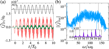
Figure 4: Results in the spinless-fermion model in the cw field. (a) Time profiles of $A(t)$ (upper) and $\langle\hat{j}\rangle_{t}$ [red (light gray) line in lower]. The green (dark gray) line in lower represents $\langle\hat{j}\rangle_{t}$ where the inter-dimer current is only taken into account. (b) Fourier transform of the current, $\langle\hat{j}\rangle_{\omega}$. Inset shows an enlargement. We set $V^{\prime}/(4t_{0})=2.4$, $V_{0}/V^{\prime}=1$, $t^{\prime}/t_{0}=0.5$, $A_{0}=5.8$, $\omega_{0}/t_{0}=0.1$, and $\tau=1/\omega_{0}$. The iTEBD method is utilized.

Now, a microscopic process of the HHG is explained by the adiabatic many-body energy diagram in Fig. 3(a). Let us start from the all-up state, $|\cdots\uparrow\uparrow\uparrow\uparrow\uparrow\cdots\rangle$, at $E_{s}=0$ as a symmetry-broken GS. The first excited state at $E_{s}=0$ is given by a liner combination of the single kink-antikink excitation states, and is adiabatically connected to $|\cdots\downarrow\downarrow\uparrow\downarrow\downarrow\cdots\rangle$ in the limit of $E_{s}\rightarrow-\infty$. With decreasing $E_{s}$ from zero, the energy level of the all-up state increases and anticrosses with the excited state [(1) in Figs. 3(a) and (b)]. This anticrossing point is known as the quantum spinodal point raedt ; miyashita . Through the Landau-Zener transition, the state which is adiabatically connected to the all-up state transfers with finite probability to the excited state $|\cdots\downarrow\downarrow\uparrow\downarrow\downarrow\cdots\rangle$ at a certain negative $E_{s}$. However, the transition amplitude $\langle\phi_{0}(E_{s})|\hat{j}|\phi_{i}(E_{s})\rangle$ is almost zero between the all-up state and this excited state, since the current operator proportional to $\sum_{i}\sigma_{i}^{y}$ brings about one PS flip. When a sign of $E(t)$ is turned into positive, the excited state moves adiabatically [(2) in Figs. 3(a) and (b)], and is changed into $|\cdots\uparrow\uparrow\downarrow\uparrow\uparrow\cdots\rangle$ at large positive $E_{s}$. The transition amplitude $\langle\phi_{0}(E_{s})|\hat{j}|\phi_{i}(E_{s})\rangle$ is finite between this excited state and the initial GS, and the system returns to the initial state accompanied by light emission [(3) in Figs. 3(a) and (b)]. This description based on the many-body states corresponds to the three-step model known for the atoms and semiconductors, and is valid at least in the region where $A_{0}$ is close to the threshold and $V^{\prime}/(4t_{0})\gtrsim 2.4$.

So far, effects of the electron itineracy is neglected on the HHG spectra calculated in the TI model, where the inter-dimer hoppings are not taken into account. It is widely recognized that, in Mott insulators as well as conventional semiconductors the electron itineracy due to the inter-site hopping integral is essential for HHG silva ; murakami . Beyond the TI model, we analyze the HHG in the interacting fermion model given in Eq. (1), where the polar CO state is realized for $V^{\prime}\gg t_{0},t^{\prime}$. A time profile of $\langle\hat{j}\rangle_{t}$ is shown in Fig. 4(a) where we set $t^{\prime}=0.5t_{0}$, and $\langle\hat{j}\rangle_{\omega}$ is shown in Fig. 4(b). Amplitude of the electric current is dominated by the intra-dimer component, and contribution from the inter-dimer current is less than $10\%$ (see green line in Fig 4(a)), although amplitude of $t^{\prime}$ is chosen to be half of $t_{0}$. We conclude that the essential characters in the HHG in the polar CO state is not governed by the electron propagation over the dimer units, but by the kind-antikink excitations and propagations.

In summary, we investigated HHG in the spontaneously symmetry-broken state realized in the TI model and the spinless-fermion model as the effective models of the interacting electrons in a dimer-type lattice structure. The kink-antikink dynamics are responsible for the present HHG, instead of the electron itineracy. The many-body character in the wavefunction governs the transition amplitude between GS and excited states. Experimental observations are crucial to confirm the present theoretical prediction for a new mechanism of HHG. Candidate materials are low-dimensional organic molecular solids, (TMTTF)₂X (TMTTF=Tetramethyltetrathiafulvalene, X=PF₆, AsF₆), which show the polar CO phase in low temperatures javadi ; monceau ; iwai .

- (1) U. Huttner, M. Kira, and S. W. Koch, Laser Photonics Rev. 11, 1700049 (2017).
- (2) S. Y. Kruchinin, F. Krausz, and V. S. Yakovlev, Rev. Mod. Phys. 90, 021002 (2018).
- (3) S. Ghimire and D. A. Reis, Nat. Phys. 15, 10 (2019).
- (4) P. Agostini and L. F. DiMauro, Rep. Prog. Phys. 67, 813 (2004).
- (5) F. Krausz and M. Ivanov, Rev. Mod. Phys. 81, 163 (2009).
- (6) L. Gallmann, C. Cirelli, and U. Keller, Annu. Rev. Phys. Chem. 63, 447 (2012).
- (7) P. B. Corkum, Phys. Rev. Lett. 71, 1994 (1993).
- (8) M. Lewenstein, P. Balcou, M. Y. Ivanov, A. L’Huillier, and P. B. Corkum, Phys. Rev. A 49, 2117 (1994).
- (9) K. L. Ishikawa and T. Sato, IEEE J. Sel. Top. Quantum Electron. 21, 8700916 (2015).
- (10) S. Ghimire, A. D. DiChiara, E. Sistrunk, P. Agostini, L. F. DiMauro, and D. A. Ries, Nat. Phys. 7, 138 (2011).
- (11) M. Hohenleutner, F. Langer, O. Schubert, M. Knorr, U. Huttner, S. W. Koch, M. Kira, and R. Huber, Nature 523, 572 (2015).
- (12) G. Ndabashimiye, S. Ghimire, M. Wu, D. A. Browne, K. J. Schafer, M. B. Gaarde, and D. A. Reis, Nature 534, 520 (2016).
- (13) H. Liu, Y. Li, Y. S. You, S. Ghimire, T. F. Heinz, and D. A. Reis, Nat. Phys. 13, 262 (2017).
- (14) N. Yoshikawa, T. Tamaya, and K. Tanaka, Science 356, 736 (2017).
- (15) T. Higuchi, M. I. Stockman, and P. Hommelhoff, Phys. Rev. Lett. 113, 213901 (2014).
- (16) P. G. Hawkins, M. Y. Ivanov, and V. S. Yakovlev, Phys. Rev. A 91, 013405 (2015).
- (17) G. Vampa, C. R. McDonald, G. Orlando, P. B. Corkum, and T. Brabec, Phys. Rev. B 91, 064302 (2015).
- (18) C. R. McDonald, G. Vampa, P. B. Corkum, and T. Brabec, Phys. Rev. A 92, 033845 (2015).
- (19) M. Wu, D. A. Browne, K. J. Schafer, and M. B. Gaarde, Phys. Rev. A 94, 063403 (2016).
- (20) T. Ikemachi, Y. Shinohara, T. Sato, J. Yumoto, M. Kuwata-Gonokami, and K. L. Ishikawa, Phys. Rev. A 95, 043416 (2017).
- (21) K. K. Hansen, T. Deffge, and D. Bauer, Phys. Rev. A 96, 053418 (2017).
- (22) T. Ikemachi, Y. Shinohara, T. Sato, J. Yumoto, M. Kuwata-Gonokami, and K. L. Ishikawa, Phys. Rev. A 98, 023415 (2018).
- (23) T. N. Ikeda, K. Chinzei, and H. Tsunetsugu, Phys. Rev. A 98, 063426 (2018).
- (24) S. Y. Kruchinin, arXiv:1806.05556.
- (25) H. Kishida, H. Matsuzaki, H. Okamoto, T. Manabe, M. Yamashita, Y. Taguchi, and Y. Tokura, Nature 405, 929 (2000).
- (26) T. Ogasawara, M. Ashida, N. Motoyama, H. Eisaki, S. Uchida, Y. Tokura, H. Ghosh, A. Shukla, S. Mazumdar, and M. Kuwata-Gonokami, Phys. Rev. Lett. 85, 2204 (2000).
- (27) R. E. F. Silva, I. V. Blinov, A. N. Rubtsov, O. Smirnova, and M. Ivanov, Nat. Photonics 12, 266 (2018).
- (28) Y. Murakami, M. Eckstein, and P. Werner, Phys. Rev. Lett. 121, 57405 (2018).
- (29) N. Tancogne-Dejean, M. A. Sentef, and A. Rubio, Phys. Rev. Lett. 121, 97402 (2018).
- (30) S. Takayoshi, Y. Murakami, and P. Werner, Phys. Rev. B 99, 184303 (2019).
- (31) W. Zhu, A. Chacon, and J. Zhu, arXiv:1811.12334
- (32) H. Kino, and H. Fukuyama, J. Phys. Soc. Jpn. 65, 2158 (1996).
- (33) M. Naka and S. Ishihara, J. Phys. Soc. Jpn. 79, 063707 (2010).
- (34) C. Hotta, Phys. Rev. B 82, 241104(R) (2010).
- (35) M. Tsuchiizu (private communication).
- (36) Derivation of the effective models and introduction of the light field in the models are explained in more detail in the Supplemental Material.
- (37) P. Pfeuty, Ann. Phys. 57, 79 (1970).
- (38) G. Vidal, Phys. Rev. Lett. 98, 070201 (2007).
- (39) H. De Raedt, S. Miyashita, K. Saito, D. García-Pablos and N. García, Phys. Rev. B 56, 11761 (1997).
- (40) S. Miyashita, K. Saito, and H. De Raedt, Phys. Rev. Lett. 80, 1525 (1998).
- (41) H. H. S. Javadi, R. Laversanne, and A. J. Epstein, Phys. Rev. B 37, 4280 (1988).
- (42) P. Monceau, F. Ya. Nad, and S. Brazovskii, Phys. Rev. Lett. 86, 4080 (2001).
- (43) Y. Naitoh, Y. Kawakami, T. Ishikawa, Y. Sagae, H. Itoh, K. Yamamoto, T. Sasaki, M. Dressel, S. Ishihara, Y. Tanaka, K. Yonemitsu, and S. Iwai, Phys. Rev. B 93, 165126 (2016).