Quantum critical scaling and holographic bound for transport coefficients near Lifshitz points

Abstract

The transport behavior of strongly anisotropic systems is significantly richer compared to isotropic ones. The most dramatic spatial anisotropy at a critical point occurs at a Lifshitz transition, found in systems with merging Dirac or Weyl point or near the superconductor-insulator quantum phase transition. Previous work found that in these systems a famous conjecture on the existence of a lower bound for the ratio of a shear viscosity to entropy is violated, and proposed a generalization of this bound for anisotropic systems near charge neutrality involving the electric conductivities. The present study uses scaling arguments and the gauge-gravity duality to confirm the previous analysis of universal bounds in anisotropic Dirac systems. We investigate the strongly-coupled phase of quantum Lifshitz systems in a gravitational Einstein-Maxwell-dilaton model with a linear massless scalar which breaks translations in the boundary dual field theory and sources the anisotropy. The holographic computation demonstrates that some elements of the viscosity tensor can be related to the ratio of the electric conductivities through a simple geometric ratio of elements of the bulk metric evaluated at the horizon, and thus obey a generalized bound, while others violate it. From the IR critical geometry, we express the charge diffusion constants in terms of the square butterfly velocities. The proportionality factor turns out to be direction-independent, linear in the inverse temperature, and related to the critical exponents which parametrize the anisotropic scaling of the dual field theory.

1 Introduction

Bounds on transport coefficients are an important tool to quantify the strength of correlations in quantum many-body systems. If one can identify a theoretical value for a minimal electrical conductivity or viscosity, then one can judge how strongly-interacting a system is. A highly influential bound for momentum conserving scattering of quantum fluids was proposed by Kovtun, Son, and Starinets Kovtun2005 (KSS) for the ratio of the shear viscosity and entropy density

$$\eta/s\geq\frac{\hbar}{4\pi k_{{\rm B}}}.$$ (1)

It is obeyed in systems like the quark gluon plasma Schaefer2014 or cold atoms in the unitary scattering limit Thomas2009 . Graphene at charge neutrality is another example that is expected to be close to this bound Mueller2009 . Within the Boltzmann transport theory one finds that a bound for $\eta/s$ can be related to the ratio $l_{{\rm mfp}}/\lambda$ of the mean-free path $l_{{\rm mfp}}$ and the mean distance $\lambda$ between carriers. However, Eq.(1) is valid even for systems that cannot be described in terms of the quasi-classical Boltzmann theory. Indeed, the bound is saturated for quantum field theories in the strong coupling limit as was shown in Ref.Kovtun2005 using the holographic duality of conformal field theory and gravity in anti-de-Sitter spacetime Maldacena1998 ; Witten1998 ; Gubser1998 .
Limiting bounds for the charge transport like the electrical conductivity are somewhat more subtle. A much discussed example is the Mott-Ioffe-Regel limit Ioffe1960 ; Mott1972 ; Gurvitch1981 that corresponds to a threshold value of the electrical resistivity when $l_{{\rm mfp}}/\lambda\sim{\cal O}\left(1\right)$. While some systems clearly show a saturation of the resistivity once $\lambda/l_{{\rm mfp}}$ reaches unity, materials like the cuprate or iron-based superconductors violate this limit Emery1995 . For a detailed discussion of correlated materials that obey or systematically violate the Mott-Ioffe-Regel bound, see Ref.Hussey2004 . Transport properties in quantum critical systems were argued under certain circumstances to be governed by a Planckian relaxation rate $\hbar\tau^{-1}\approx k_{\text{B}}T$ Zaanen2004 ; Sachdev2011 , which would also limit the electrical conductivity at quantum critical points. A bound on charge transport that is less restrictive and theoretically better justified than the Mott-Ioffe-Regel limit was proposed in Ref.Hartnoll2015 . It constrains the value of the charge diffusivity:

$$D_{c}\geq C_{D}\frac{\hbar v^{2}}{k_{{\rm B}}T},$$ (2)

with $C_{D}$ is a numerical coefficient of order unity. Here $v$ is a characteristic velocity of the problem. At charge neutrality the heat and electric currents are decoupled, and the charge diffusivity is determined by the Einstein relation $D_{c}=\sigma/{\chi}_{\rho}$. $\sigma$ is the electrical conductivity, and ${\chi}_{\rho}=\partial\rho/\partial\mu$ the charge susceptibility with particle density $\rho$ and chemical potential $\mu$. The latter is related to the charge compressibility since ${\chi}_{\rho}=-\frac{\rho^{2}}{V}\frac{\partial V}{\partial p}$. If $v^{2}{\chi}_{\rho}$ stays constant as $T\rightarrow 0$, the electrical resistivity cannot vanish slower than linearly in $T$ Hartnoll2015 . Ref.Blake2016 ; Blake2016b proposed the butterfly velocity $v=v_{\mathrm{B}}$ as the characteristic velocity. $v_{\mathrm{B}}$ follows from the analysis of out-of-time-order (OTOC) correlations $C\left(\mathbf{x},t\right)=-\left\langle\left[A\left(\mathbf{x},t\right),B\left(\mathbf{0},0\right)\right]^{2}\right\rangle$ that are discussed in the context of chaos and information scrambling Shenker2014 ; Shenker2015 ; Roberts2015 ; Roberts2016 ; Maldacena2016 . It can be obtained from the long-distance behavior, e.g. via

$$C\left(\mathbf{x},t\right)\sim e^{2\lambda_{\text{L}}\left(t-\frac{\mathbf{\left|x\right|}}{v_{\mathrm{B}}}\right)}.$$ (3)

The scrambling rate $\lambda_{\text{L}}$ that enters the OTOC is also subject to the bound $\lambda_{\text{L}}\leq 2\pi k_{\text{B}}T/\hbar$ Maldacena2016 . While the interpretation of $\lambda_{\text{L}}$ and its relation to transport and thermalization rates is not always correct Blake:2017qgd ; Klug2018 ; Davison:2018ofp ; Davison2018 ; 1710.00921 ; 1706.00019 , the butterfly velocity seems to yield a natural scale for the characteristic velocity of a system, even if no clear quasiparticle description is available. A caveat applies when a symmetry of the system is weakly broken and triggers a sound-to-diffusion crossover: in this case, the resulting diffusivity is more naturally expressed in terms of the sound velocity and the gap Davison2015b ; Davison:2018ofp ; Grozdanov:2018fic .

The focus of this paper is the investigation of anisotropic systems, where the conductivity tensor $\sigma_{\alpha\beta}$ and the viscosity tensor $\eta_{\alpha\beta\gamma\delta}$ exhibit a more complex structure with potentially different temperature dependencies for distinct tensor elements Cook2019 ; Link2018 . The anisotropy that we consider is most naturally expressed in terms of the relation between characteristic energies and momenta along different directions. For a system with two space dimensions, it holds then that:

$$\omega \sim \left|k_{x}\right|^{z/\phi}$$

$$\omega \sim \left|k_{y}\right|^{z}$$ (4)

with dynamical exponent $z$. We characterize the anisotropy in terms of the exponent $\phi$ that relates typical momenta along the two directions according to

$$\left|k_{x}\right|\sim\left|k_{y}\right|^{\phi}.$$ (5)

A single particle dispersion that is consistent with such scaling would be $\varepsilon\left(\mathbf{k}\right)\sim\left|k_{x}\right|^{z/\phi}+a\left|k_{y}\right|^{z}$ that corresponds to a system at a Lifshitz point Lifshitz1942 ; Dzyaloshinski1964 ; Goshen1974 ; Hornreich1975 ; PhysRevB.62.12338 ; SHPOT2001340 ; Shpot_2005 ; 0802.2434 . However, our conclusions do not require the existence of well defined quasiparticles with this dispersion relation.

Anisotropic systems, that obey scaling behavior of a Lifshitz transition were recently shown to violate the viscosity bound Rebhan2012 ; Jain2015 ; Ge:2014aza ; Ge2017 ; Link2018 ; 1805.01470 ; Ge:2014aza ; 1205.1797 ; 1306.1404 ; Pedraza2018 . In Ref.Link2018 a model of anisotropic Dirac fermions that emerged from two ordinary Dirac cones was analyzed as an explicit condensed matter realization Isobe2016 . Within a quasiparticle description of the transport processes and a Boltzmann equation approach, the conductivity anisotropy was found to diverge: one direction is metallic and another one insulating. Based on the quasiparticle transport theory, a modified bound was conjectured, that involves not just the viscosity tensor elements $\eta_{\alpha\beta\alpha\beta}$ and the entropy density $s\left(T\right)$, but also the conductivities Link2018 :

$$\frac{\eta_{\alpha\beta\alpha\beta}}{s}\frac{\sigma_{\beta\beta}}{\sigma_{\alpha\alpha}}\geq\frac{\hbar}{4\pi k_{{\rm B}}}.$$ (6)

Here, no summation over repeated indices is implied.
Other tensor elements like $\eta_{\alpha\beta\beta\alpha}$ continue to obey Eq.(1). The origin for this combined viscosity-conductivity bound is the different scaling behavior of the typical velocities $v_{\alpha}$ for different directions. Candidate materials with Lifshitz transitions are the organic conductor $\alpha-(\text{BEDT-TTF}_{2})\text{I}_{3}$ under pressure Julia27 , and the heterostructure of the $5/3\text{TiO}_{2}/\text{VO}_{2}$ supercell Julia28 ; Julia29 . Moreover, the surface modes of topological crystalline insulators with unpinned surface Dirac cones Julia30 and quadratic double Weyl fermions Julia31 are expected to exhibit such a behavior.

The analysis of Ref.Link2018 was based on the Boltzmann equation and did not allow to explicitly analyze a model that satisfies this bound or determine the precise numerical coefficient in Eq.(6), i.e. the factor ${1}/{4\pi}$. This can only be done within a formalism that addresses transport in strongly-coupled non-quasi-particle many-body systems. In the same context it is of interest to address the related question of whether the diffusivity bound, Eq.(2), is also modified for anisotropic systems.

In this paper we perform a holographic analysis of anisotropic transport, exploiting the duality between strongly coupled quantum field theories in $d+1$ dimensions and gravity theories in one additional dimension Maldacena1998 . The calculation is based on an Einstein-Maxwell-dilaton (EMD) action, where the anisotropy is generated by massless scalars, linear in the boundary spatial coordinates. See Refs. Rebhan2012 ; Jain2015 ; Ge:2014aza ; 1306.1404 ; Jeong2018 ; Donos:2014uba ; Ge2017 ; Mateos:2011ix ; Mateos:2011tv ; 1205.1797 ; Pedraza2018 ; Donos2014 ; 1202.4436 for previous studies of these holographic systems. As a consequence, the scalars also break translations and momentum is not conserved. If the symmetry breaking occurs explicitly, the viscosity cannot be interpreted as a hydrodynamic coefficient. It is well known that in such holographic frameworks the KSS bound is violated Rebhan2012 ; Jain2015 ; Ge:2014aza ; Ge2017 ; 1805.01470 ; Ge:2014aza ; 1205.1797 ; 1306.1404 ; Pedraza2018 ; Hartnoll2016 ; Alberte:2016xja ; Ciobanu:2017fef ; Burikham2016 ; Ling_2016 ; Ling_2017 ; 1510.06861 .
We will also investigate the case where translations are broken spontaneously through the use of a so-called Q-lattice homogeneous Ansatz Amoretti2018_CDW ; Amoretti:2017axe ; 1904.11445 , in which case momentum is still conserved and the shear viscosity remains well-defined at all temperatures.
As our focus in this work is on the anisotropy of the system, we will choose a geometry where momentum is conserved along one of the spatial directions, say the $\beta$-direction. Thus, the stress tensor elements $T_{\alpha\beta}$ serves as currents of the conserved momentum density along the direction $\beta$. Consequently, the viscosity elements $\eta_{\alpha\beta\gamma\beta}$ maintain their meaning as hydrodynamic coefficients, for all $\alpha$ and $\gamma$.

We compute the anisotropic electric conductivities in this holographic system, and find that, at charge neutrality, their ratio is given by a simple geometric ratio of the spatial elements of the bulk metric evaluated at the bulk black hole horizon. Their temperature dependence indicates metallic behavior along one spatial direction and insulating behavior along the other, as in Ref.Link2018 .

Returning to the viscosities, we find that in the direction where momentum is conserved, the viscosity matrix elements are governed by the same geometric ratio as the electric conductivities, so that, Link2018 :

$$\frac{\eta_{\alpha\beta\alpha\beta}}{s}=\frac{\hbar}{4\pi k_{\text{B}}}\frac{\sigma_{\alpha\alpha}}{\sigma_{\beta\beta}}.$$ (7)

The generalized bound Eq.(7) has to be understood as a relation between hydrodynamic coefficients, which holds at all temperatures, including the low temperature regime where the anisotropy is large. Moreover, the combination $\frac{\eta_{\alpha\beta\alpha\beta}}{s}\frac{\sigma_{\beta\beta}}{\sigma_{\alpha\alpha}}$ serves as an indicator of strong coupling behavior in anisotropic systems. In Fig.1 we show typical temperature dependencies for these transport coefficients for a specific value of the crossover exponent $\phi$ that characterizes the anisotropy. When translations are broken along the $\beta$-direction, $\eta_{\alpha\beta\gamma\beta}$ loses its hydrodynamic meaning and just gives the stress-tensor correlation function. The tensor element satisfies a holographic relation which we analyze in both the limits of high and low temperature.

In addition, we determine the anisotropic butterfly velocity $v_{B,\alpha}$ (see Refs. 1805.01470 ; Jeong2018 ; Pedraza2018 ; 1610.02669 ; Blake:2017qgd ; 1710.05765 ; 1708.07243 ; 1811.06949 for previous studies) and the compressibility, and obtain for the anisotropic diffusivity the generalization of Eq.(2)

$$D_{c,\alpha}=\frac{d_{\text{eff}}-\theta}{\Delta_{\chi}}\frac{\hbar v_{B,\alpha}^{2}}{2\pi k_{{\rm B}}T},$$ (8)

where $d_{\text{eff}}$ is the effective spatial dimensionality – see Eq.(11) below, $\theta$ the hyperscaling violating exponent, and $\Delta_{\chi}$ the scaling dimension of the charge susceptibility. Thus, the bound of Eq.(2) can be generalized to anisotropic systems. In distinction to the viscosity bound, the anisotropy only changes the universal coefficient that now depends on the exponents $\phi,z,$ and $\theta$. Furthermore, (8) recovers the limit of isotropic charge neutral theories Blake2016 . In Ref.Jeong2018 , the thermal diffusivity was computed in anisotropic setups and also found to obey a relation similar to (8). See Ref.1805.01470 for an alternative proposal to (8) at an anisotropic QCP.

Before we present the theories that yield these results, we give some general scaling arguments, assuming charge and momentum conservation. This analysis motivates us to consider the appropriate combinations of transport quantities that enter Eq.(6) and Eq.(8). The scaling analysis is then followed by a holographic analysis of the combined viscosity-conductivity bound, the charge susceptibility, and the butterfly velocity within an anisotropic gravity theory.

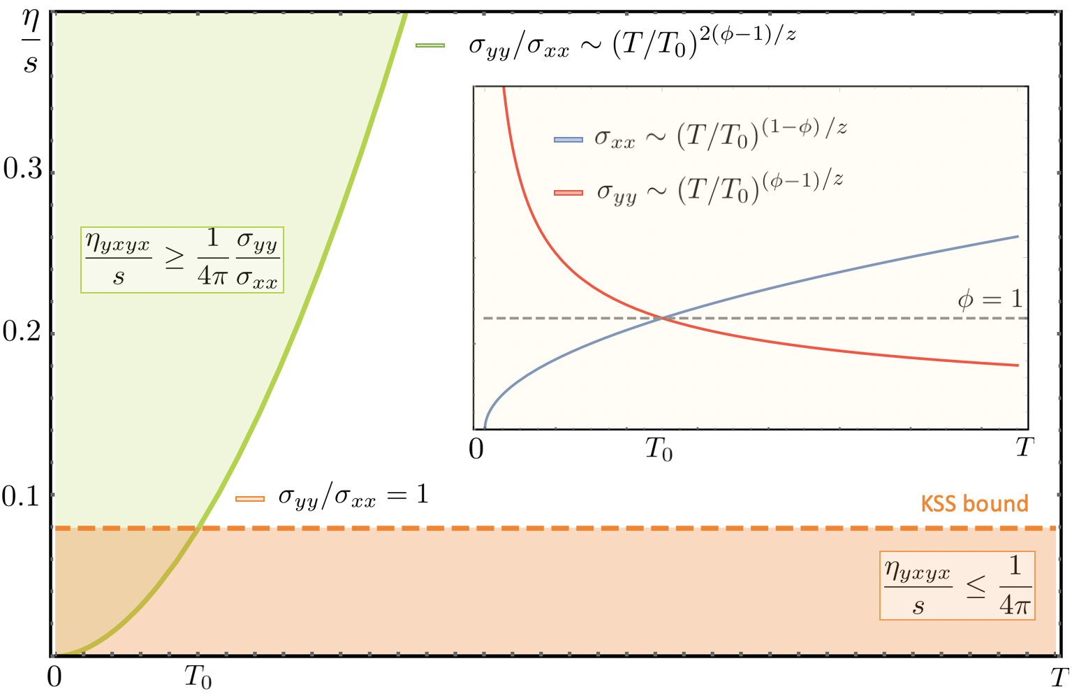
Figure 1: Main panel: temperature dependence of the $\eta/s$ tensor. In the anisotropic case the KSS bound (orange) can be parametrically violated (green line). Here, $T_{0}$ is a temperature scale below which the anisotropy effects are dominant. The conductivity ratio might constitute a new lower bound when rotations are broken (green). Inset: temperature dependence of the conductivity tensor elements $\sigma_{xx}$ and $\sigma_{yy}$. $\phi$ is the crossover exponent that characterizes the anisotropy between the different spatial directions $k_{x}\sim k_{y}^{1/\phi}$. Once $\phi\neq 0$ one element of the conductivity of a two-dimensional system must be insulating and the other must be metallic.

2 Scaling arguments

We consider the scaling behavior of transport coefficients in anisotropic systems near a quantum critical Lifshitz point. As we will see, scaling arguments can be efficiently used to make statements about transport bounds. Once a combination of physical observables has scaling dimension zero, it naturally approaches a universal value in the limit $T,\mu,\omega\cdots\rightarrow 0$, that corresponds to an underlying quantum critical state. If one can argue, usually based on an analysis of conservation laws, that this value is neither zero nor infinity, it should be some dimensionless number times the natural unit of the observable. In other words, this combination should be insensitive to irrelevant deformations of the quantum critical point. As an example we consider the electrical conductivity at zero density. For isotropic systems its scaling dimension is $d-2$, a result that follows from single-parameter scaling and charge conservation. Thus the conductivity of a zero density two-dimensional system is expected to reach a universal value in units of the natural scale $e^{2}/h$. Under the same conditions, both the viscosity and the entropy density have scale dimension $d$ such that their ratio has scaling dimension zero. Then $\eta/s$ should approach a universal value times $\hbar/k_{{\rm B}}$ which yields the correct physical unit. This observation helps to rationalize a result like Eq.(1). As an aside, these scaling considerations also offer a natural explanation why the bound Eq.(1), while applicable, is not very relevant for Fermi liquids. Here, the existence of a large Fermi surface gives rise to hyper-scaling violating exponents Huijse:2011ef . If one performs the appropriate scaling near the Fermi surface Shankar1994 , then it seems more natural to use $\eta s^{2}$ as the natural bound, a quantity that approaches a constant value as $T\rightarrow 0$.

The conclusions of this section require that scaling relations are valid, i.e that the system under consideration behaves critical and is below its upper critical dimension. In the remainder of this section we assume that this is the case. To be specific, we analyze a $d$-dimensional system and allow for one direction to be governed by a characteristic length scale with a different scaling dimension $\phi\neq 1$ than the other spatial directions, see Eqs.(4,5) above. In addition, the temporal direction is characterized by a dynamic scaling exponent $z$. Let us then consider a physical observable $O\left(\mathbf{k},\omega\right)$. By assumption the observable obeys the scaling relation

$$O\left(k_{\perp},\mathbf{k}_{\parallel},\omega\right)=b^{-\Delta_{O}}O\left(b^{\phi}k_{\perp},b\mathbf{k}_{\parallel},b^{z}\omega\right).$$ (9)

Here $\Delta_{O}$ is the scaling dimension of the observable. The $d$-dimensional momentum vector $\mathbf{k}=\left(k_{\perp},\mathbf{k}_{\parallel}\right)$ consists of one component $k_{\perp}$ that is governed by the exponent $\phi$ and a $d-1$ dimensional component $\mathbf{k}_{\parallel}$. In the subsequent holographic analysis we focus on a system with two spatial coordinates and use the notation $k_{\perp}=k_{x}$ and $k_{\parallel}=k_{y}$. While the scaling analysis presented here cannot determine the values of the exponents, it allows for rather general conclusions once those exponents are known. For an explicit model with nontrivial exponents $z$ and $\phi$, see Ref.Link2018 .

2.1 Scaling of thermodynamic quantities

We begin our discussion of scaling laws with thermodynamic quantities. For the free-energy density of the system holds the following scaling law:

$$F\left(T,\mu\right)=b^{-d_{{\rm eff}}-z}F\left(b^{z}T,b^{z}\mu\right),$$ (10)

with effective dimension

$$d_{{\rm eff}}=d-1+\phi.$$ (11)

As an energy density, $F$ should scale like unit energy per unit volume. To obtain its scaling dimension it is then easiest to start from the usual result $d+z$ for isotropic systems Sachdev2011 and replace $d$ by $d_{{\rm eff}}$. This takes into account the different weight of the directions $\mathbf{k}_{\parallel}$ and $k_{\perp}$. With $s=-\partial F/\partial T$ and $\rho=\partial F/\partial\mu$ we obtain immediately the scaling dimensions

$$\Delta_{s}=\Delta_{\rho}=d_{{\rm eff}}$$ (12)

for the entropy density $s$ and particle density $\rho$, respectively. Away from zero density, the relation $\Delta_{\rho}=d_{{\rm eff}}$ generally does not hold Gouter_2014_mom_diss ; Hartnoll2015-1 ; Davison:2018ofp . The second derivative of the free energy with respect to the chemical potential yields charge susceptibility

$${\chi}_{\rho}\left(T,\mu\right)=b^{-\Delta_{\chi}}{\chi}_{\rho}\left(b^{z}T,b^{z}\mu\right)$$ (13)

with $\Delta_{\chi}=d_{{\rm eff}}-z$. We can now use these thermodynamic relations to determine the scaling behavior of the conductivity and viscosity. To do so is possible because of the restrictions that follow from charge and momentum conservation.

2.2 Scaling of transport coefficients

The conductivity is determined via a Kubo formula from the current-current correlation function, e.g.

$${\rm Re}\,\sigma_{\alpha\beta}\left(\omega\right)=\frac{{\rm Im}\,\Pi_{\alpha\beta}\left(\omega\right)}{\omega}.$$ (14)

At zero density, the system has a finite d.c. conductivity. $\Pi_{\alpha\beta}\left(\omega\right)$ is the Fourier transform of the retarded current-current correlation function $\Pi_{\alpha\beta}\left(t\right)=-i\theta\left(t\right)\left\langle\left[j_{\alpha}\left(t\right),j_{\beta}\right]\right\rangle$. In order to exploit the implications of charge conservation we use the continuity equation

$$\partial_{t}\rho+\partial_{\alpha}j_{\alpha}=0$$ (15)

and obtain the well known relation between the longitudinal conductivity $\sigma_{\alpha\alpha}\left(\omega\right)$ and the density-density correlation $\bar{\chi}_{\rho}\left(\mathbf{k},\omega\right)$

$$\sigma_{\alpha\alpha}\left(\omega\right)=\lim_{\mathbf{k}\rightarrow 0}\frac{\omega}{k_{\alpha}^{2}}\bar{\chi}_{\rho}\left(\mathbf{k},\omega\right).$$ (16)

Here $\bar{\chi}_{\rho}\left(\mathbf{k},\omega\right)$ is the temporal Fourier transform of $\bar{\chi}_{\rho}\left(\mathbf{k},t\right)=-i\theta\left(t\right)\left\langle\left[\rho\left(\mathbf{k},t\right),\rho\left(-\mathbf{k},0\right)\right]\right\rangle$, where $\rho\left(\mathbf{k},t\right)$ is the spatial Fourier transform of the density $\rho\left(\mathbf{x},t\right)$. Since ${\chi}_{\rho}=\lim_{\mathbf{k}\rightarrow 0}\bar{\chi}_{\rho}\left(\mathbf{k},\omega=0\right)$, the scaling dimension of ${\chi}_{\rho}$ is also $\Delta_{\chi}$, given below Eq.(13). Thus we find

$$\Delta_{\sigma,\parallel} = \Delta_{\chi}+z-2=d_{{\rm eff}}-2,$$

$$\Delta_{\sigma,\perp} = \Delta_{\chi}+z-2\phi=d_{{\rm eff}}-2\phi,$$ (17)

for the conductivities along the two directions. This yields for the conductivities:

$$\sigma_{\parallel}\left(T,\omega\right) = b^{3-\phi-d}\sigma_{\parallel}\left(b^{z}T,b^{z}\omega\right),$$

$$\sigma_{\perp}\left(T,\omega\right) = b^{\phi+1-d}\sigma_{\perp}\left(b^{z}T,b^{z}\omega\right).$$ (18)

If we return to the isotropic limit, where $\phi=1$, both components of the conductivity behave the same with usual conductivity scaling dimension $d-2$. Interestingly, in the anisotropic case, this continues to be the dimension of the geometric mean $\sqrt{\sigma_{\parallel}\sigma_{\perp}}$. Distinct scaling exponents for the tensor elements imply a different temperature dependency of the conductivity for different directions. Thus, a more insulating behavior along one direction will force the other direction to be more metallic. For a two-dimensional system, one direction will have to be insulating and the other then has to be metallic as long as $\phi\neq 1$. Finally, the ratio $\sigma_{\parallel}/\sigma_{\perp}$ of the conductivity is governed by $\Delta_{\sigma,\parallel}-\Delta_{\sigma,\perp}=2\left(\phi-1\right)$, i.e.

$$\frac{\sigma_{\parallel}\left(T\right)}{\sigma_{\perp}\left(T\right)}=b^{-2\left(\phi-1\right)}\frac{\sigma_{\parallel}\left(b^{z}T\right)}{\sigma_{\perp}\left(b^{z}T\right)}.$$ (19)

We can perform a similar analysis for the viscosity tensor. It is given by a different Kubo formula

$${\rm Re}\,\eta_{\alpha\beta\gamma\delta}\left(\omega\right)=\frac{{\rm Im}\,\Pi_{\alpha\beta\gamma\delta}\left(\omega\right)}{\omega},$$ (20)

with $\Pi_{\alpha\beta\gamma\delta}\left(\omega\right)$ the Fourier transform of the retarded stress-tensor correlation function $\Pi_{\alpha\beta\gamma\delta}\left(t\right)=-i\theta\left(t\right)\left\langle\left[T_{\alpha\beta}\left(t\right),T_{\gamma\delta}\right]\right\rangle$. Momentum conservation gives rise to the continuity equation for the momentum density $g_{\alpha}\equiv T^{0}_{\alpha}$:

$$\partial_{t}g_{\beta}+\partial_{\alpha}T_{\alpha\beta}=0.$$ (21)

We are considering a system without rotation invariance. In this case it is important to keep track of the order of the tensor indices as $T_{\alpha\beta}$ cannot be brought into a symmetric form Link2018b . From the continuity equation for the momentum follows for the viscosity

$$\eta_{\alpha\beta\gamma\delta}\left(\omega\right)=\lim_{\mathbf{k}\rightarrow 0}\frac{\omega}{k_{\alpha}k_{\gamma}}\chi_{\beta\delta}^{\left(g\right)}\left(\mathbf{k},\omega\right),$$ (22)

with momentum-density correlation function $\chi_{\beta\delta}^{\left(g\right)}\left(\mathbf{k},\omega\right)$, i.e. the Fourier transform of $\chi_{\beta\delta}^{\left(g\right)}\left(\mathbf{k},t\right)=-i\theta\left(t\right)\left\langle\left[g_{\beta}\left(\mathbf{k},t\right),g_{\delta}\left(-\mathbf{k},0\right)\right]\right\rangle$. Thus, we only need to know the scaling dimension of $\chi_{\beta\delta}^{\left(g\right)}$ to determine the behavior of the viscosity. The easiest way to obtain this scaling dimension is to realize that under a boost operation, a velocity field is thermodynamically conjugate to the momentum density. A velocity has scaling dimension $z-1$ for the directions along $\mathbf{k}_{\parallel}$ and $z-\phi$ for $k_{\perp}$. To capture all the options we write this as $z-\varphi_{\alpha}$ where $\varphi_{\alpha}=1$ for all directions but along $k_{\perp}$ where we have $\varphi_{\alpha}=\phi$. Thus, it holds

$$\chi_{\beta\delta}^{\left(g\right)}\left(k_{\perp},\mathbf{k}_{\parallel},\omega\right)=b^{-\Delta_{g,\beta\delta}}\chi_{\beta\delta}^{\left(g\right)}\left(b^{\phi}k_{\perp},b\mathbf{k}_{\parallel},b^{z}\omega\right).$$ (23)

with $\Delta_{g,\beta\delta}=d_{{\rm eff}}-z+\varphi_{\beta}+\varphi_{\delta}$. In the Appendix A we obtain the same behavior from an analysis of strain generators, following Refs. Link2018b ; Bradlyn2012 . Using $\Delta_{g,\beta\delta}$ allows us to determine the scaling behavior of the viscosity tensor

$$\eta_{\alpha\beta\gamma\delta}\left(T\right)=b^{-\Delta_{\eta,\alpha\beta\gamma\delta}}\eta_{\alpha\beta\gamma\delta}\left(b^{z}T\right)$$ (24)

with

$$\Delta_{\eta,\alpha\beta\gamma\delta} = \Delta_{g,\beta\delta}+z-\varphi_{\alpha}-\varphi_{\gamma}$$ (25)

$$= d_{{\rm eff}}-\varphi_{\alpha}+\varphi_{\beta}-\varphi_{\gamma}+\varphi_{\delta}.$$

For isotropic systems, this gives the well known result that the scaling dimension of the viscosity is $d$, i.e. the same as for the entropy or particle density. For an anisotropic system the scaling dimensions of the viscosity and the entropy density can still be the same. This is the case whenever $\varphi_{\alpha}+\varphi_{\gamma}=\varphi_{\beta}+\varphi_{\delta}$. Examples are $\eta_{\perp\perp\perp\perp}$, $\eta_{\perp\perp cd}$, $\eta_{ab\perp\perp}$,$\eta_{a\perp\perp d}$, or $\eta_{\perp bc\perp}$, where $a$,$b$ etc. stand for components of $\mathbf{k}_{\parallel}.$

However, the scaling dimension of the viscosity can also be different from the one of the entropy density. This is the case for

$$\eta_{a\perp c\perp}\left(T\right) = b^{-\left(d-3+3\phi\right)}\eta_{a\perp c\perp}\left(b^{z}T\right)$$

$$\eta_{\perp b\perp d}\left(T\right) = b^{-\left(d+1-\phi\right)}\eta_{\perp b\perp d}\left(b^{z}T\right).$$ (26)

If we now take the ratio of the viscosity to entropy density, we find

$$\frac{\eta_{a\perp c\perp}\left(T\right)}{s\left(T\right)} = b^{-2\left(\phi-1\right)}\frac{\eta_{a\perp c\perp}\left(b^{z}T\right)}{s\left(b^{z}T\right)},$$

$$\frac{\eta_{\perp b\perp d}\left(T\right)}{s\left(T\right)} = b^{2\left(\phi-1\right)}\frac{\eta_{\perp b\perp d}\left(b^{z}T\right)}{s\left(b^{z}T\right)}.$$ (27)

Thus, for $\phi\neq 1$ there is always one tensor element of the viscosity, where $\eta_{\alpha\beta\gamma\delta}/s$ diverges as $T\rightarrow 0$ and another one that vanishes. The latter will then obviously violate any bound for the ratio of a viscosity to entropy density. In Ref.Link2018 it was shown that precisely these tensor elements turn out to be important for the hydrodynamic Poiseuille flow of anisotropic fluids.

The origin of unconventional scaling of both the conductivities and the viscosities is geometric, i.e. rooted in the anisotropic scaling of spatial coordinates at the Lifshitz point. If one combines Eqs.(19) and (27), it is straightforward to see that the combinations that enter Eq.(6) always have scaling dimension zero. While it certainly does not offer a proof of Eq.(6) this is necessary for such quantity to approach a universal, constant low-temperature value.

Finally we comment on the scaling behavior of the diffusivity bound, Eq.(8). To check whether this bound even makes sense for an anisotropic system, we consider the quantity

$$X_{\alpha}=k_{{\rm B}}TD_{c,\alpha}/\hbar v_{\alpha}^{2}$$ (28)

where $v_{\alpha}$ is the characteristic velocity along the $\alpha$-th direction and $D_{c,\alpha}=\sigma_{\alpha\alpha}/{\chi}_{\rho}$ the diffusivity along this direction. It obviously holds

$$\Delta_{X_{\alpha}}=z+\Delta_{\sigma,\alpha}-\Delta_{\chi}-2\left(z-\varphi_{\alpha}\right)$$ (29)

where we used again that a velocity scales as $z-\varphi_{\alpha}$. If we now insert our above results, it follows

$$\Delta_{X_{\parallel}}=\Delta_{X_{\perp}}=0.$$ (30)

This implies that $X_{\alpha}$ should approach a universal constant times $\hbar/k_{{\rm B}}$. Thus, we expect Eq.(2) to be valid even for anisotropic systems, which yields Eq.(8). In this sense is this bound even more general than the original viscosity bound of Eq.(1).

3 Holographic analysis of the viscosity-conductivity bound

The correspondence between gravity theories and quantum field theories, as it occurs in the anti-de Sitter space/conformal field theory duality Maldacena1998 ; Witten1998 ; Gubser1998 , is a powerful tool to analyze the universal properties of strongly-coupled field theories. In what follows we analyze an anisotropic bulk geometry in order to determine the relationships between distinct transport coefficients of anisotropic quantum many-body problems in the strong-coupling limit. To this end we use the membrane paradigm Thorne1986 to express boundary theory transport coefficients in terms of geometric quantities at the horizon Iqbal2009 . To be specific, we consider a system of two space dimensions, i.e. with $D=2+1$ space-time coordinates at the boundary. The relation between the generating functional of the quantum field theory and the gravity action for imaginary time is given by Witten1998 ; Gubser:1998bc

$$\left\langle e^{-\int d^{3}x\Phi_{0}{O}}\right\rangle=\left.e^{-S\left[\Phi\right]}\right|_{\Phi\left(r\rightarrow 0\right)=\Phi_{0}},$$ (31)

where ${O}$ is an operator of the field theory, $\Phi_{0}$ a conjugate source, $\Phi$ the dual field, and $S$ a gravitational action in the $D+1$ dimensional bulk, with additional coordinate $r$. Here we chose a system of coordinates where the boundary lies at $r=0$. Following Ref.Iqbal2009 , retarded Green’s functions of the field theory can be obtained from

$$\left\langle{O}\left(\mathbf{x},t\right)\right\rangle_{\Phi_{0}}=\lim_{r\rightarrow 0}\Pi\left(r,\mathbf{x},t\right),$$ (32)

where $\Pi$ is the canonical momentum conjugate to $\Phi$, as follows from the gravitational version of the Hamilton-Jacobi formalism. This finally allows for the determination of retarded Green’s functions $G\left(\mathbf{x},t\right)=-i\theta\left(t\right)\left\langle\left[{O}\left(\mathbf{x},t\right),{O}\left(\mathbf{0},0\right)\right]\right\rangle.$ For the Fourier transform with respect to momentum and frequency follows

$$G\left(\mathbf{k},\omega\right)=-\lim_{r\rightarrow 0}\frac{\Pi\left(r,\mathbf{k},\omega\right)}{\Phi\left(r,\mathbf{k},\omega\right)}.$$ (33)

Causality is preserved if one considers $\Phi$ that satisfies in-falling boundary conditions at the black hole horizon Son2002 ; Herzog2003 . The related transport coefficient is given by $-\lim_{\omega,\mathbf{k}\to 0}\frac{1}{\omega}{\rm ImG\left(\mathbf{k},\omega\right)}.$

Anisotropic, static bulk geometries cannot come from a pure gravitational action. Thus, we need to couple gravity with axial gauge fields or massless scalar fields. See also Ref.1202.4436 ; 1310.6725 ; 1306.1404 for generalities on anisotropic studies in holography.
We start from the Einstein-Maxwell-dilaton action

$$S=\int d^{3+1}x\sqrt{-g}\left(R+{\cal L}_{\text{M}}\right),$$ (34)

with Lagrangian

$${\cal L}_{\text{M}}=-\frac{1}{2}\left(\nabla\varphi\right)^{2}-V\left(\varphi\right)-\frac{Y\left(\varphi\right)}{2}\left(\nabla\psi\right)^{2}-\frac{Z\left(\varphi\right)}{4}F^{2}.$$ (35)

$\varphi$ is referred to as the dilaton. It is a scalar field which enters the action modifying all the couplings involved. $V\left(\varphi\right)$ is its own potential. We include the dilaton as it will allow us to consider anisotropic geometries that arise near the horizon of near-extremal black holes. In the absence of the dilaton field, the model reduces to the usual $\text{AdS}_{4}$ system with electromagnetic field, i.e $V\left(0\right)=2\Lambda$ with cosmological constant $\Lambda=-3/\ell^{2}$, $Z\left(0\right)=1$ and $Y(0)=0$. $\ell$ is the radius of curvature of the AdS space. As we will shortly see, by considering a bulk profile that depends linearly on one of the boundary spatial coordinates, the massless scalar $\psi$ will break the rotation and translation symmetries of the dual field theory. For related work on this family of holographic models, see Refs. Mateos:2011ix ; Mateos:2011tv ; Donos:2013eha ; Andrade2014 ; Rebhan2012 ; Pedraza2018 ; Ge2017 ; Ge:2014aza ; Jain2015 ; Ling_2016 ; Ling_2017 ; Amoretti2016_chas ; Amoretti2018_CDW ; Andrade2014 ; Davison2015b ; Donos2014 ; Hartnoll2016
$F^{2}$ is the Maxwell Lagrangian with $F_{\mu\nu}=\nabla_{\mu}A_{\nu}-\nabla_{\nu}A_{\mu}$ the usual field tensor with vector potential $A_{\mu}$. This term is needed to implement a $U\left(1\right)$ global symmetry in the boundary theory and to determine the electrical conductivity.

We summarize the field equations of motion that follow from Eq.(34) varying the action with respect to the fields $g_{\mu\nu},A_{\mu},\psi,\varphi$.
Varying the metric, we obtain the Einstein equations

$$R_{\mu\nu}-\frac{1}{2}Rg_{\mu\nu}=-\frac{1}{\sqrt{-g}}\frac{\delta(\sqrt{-g}\mathcal{L}_{\text{M}})}{\delta g^{\mu\nu}}.$$ (36)

The variation of the gauge field yields the Maxwell equations

$$\partial_{\mu}(\sqrt{-g}Z(\varphi)F^{\mu\nu})=0.$$ (37)

Notice that both the scalar fields are neutral such that the Maxwell equations are bulk conservation equations for the two-form $F$. Ultimately, this will let us evaluate the boundary charge current at the black hole horizon. Finally, the wave equations for the two scalars are:

$$\partial_{\mu}(\sqrt{-g}\,Y(\varphi)\partial^{\mu}\psi)=0,$$ (38)

$$\partial_{\mu}(\sqrt{-g}\,\partial^{\mu}\varphi)={\partial_{\varphi}}V_{\text{eff}},$$ (39)

where

$$\frac{V_{\text{eff}}}{\sqrt{-g}}={V(\varphi)+\frac{Y(\varphi)}{2}(\partial\psi)^{2}+\frac{Z(\varphi)}{4}F^{2}}.$$ (40)

In the absence of external perturbations, we use the following ansatz

$$ds^{2}=-g_{tt}(r)dt^{2}+g_{rr}(r)dr^{2}+\sum_{\alpha}g_{\alpha\alpha}(r)dx_{\alpha}^{2}$$

$$\varphi=\varphi(r),\quad A=A_{t}(r)dt,\quad\psi=ay,$$ (41)

where $a$ is real and $\alpha=\{x,y\}$. The Ansatz for $\psi$ is consistent with the field equations and preserves the homogeneity of the other fields. Indeed, $\psi$ back-reacts on the equations of motion only through gradients so that all dependence on $y$ drops out of the field equations. However, translations along the $y$-direction are broken and momentum is dissipated at a strength set by $a$. On the other hand, momentum along $x$ direction is conserved which allows us to perform a hydrodynamic analysis of the viscosity tensor elements $\eta_{\alpha x\beta x}$. The metric in (41) describes anisotropic bulk geometries since, in general, $g_{xx}\left(r\right)\neq g_{yy}\left(r\right)$. The coefficient $a$ determines the temperature scale $T_{0}$ below which the anisotropy effects are large. Setting $a=0$ restores both rotations and translations in the dual field theory.

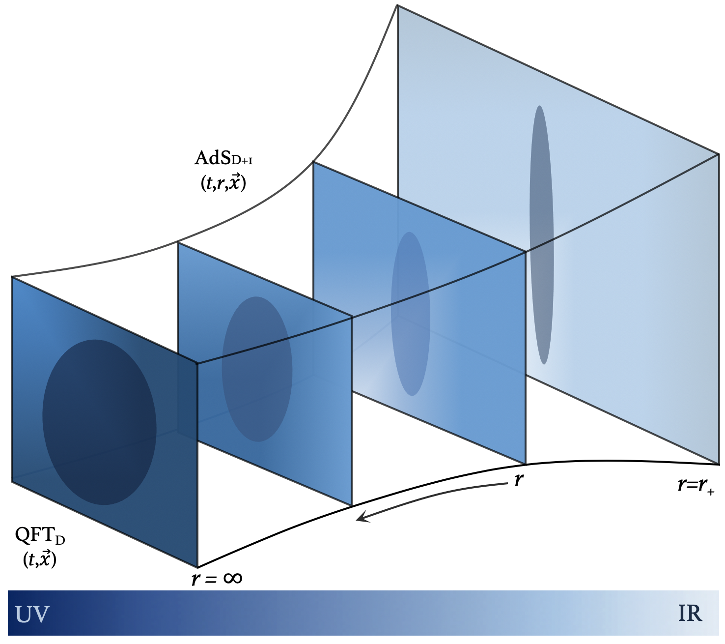
Figure 2: Cartoon of an AdS black hole geometry in ($D$+1)-spacetime dimensions. The extra coordinate $r$ is between $r=0$ and $r=r_{+}$ where the boundary and the horizon of the AdS are located, respectively. The evolution along $r$ is dual to the RG-flow of the dual $D$-spacetime dimensional QFT McGreevy . Furthermore, in order to underline how the spatial anisotropy becomes higher as one approaches the IR region, we have depicted how an ellipse is distorted in the spatial directions as $r$ decreases.

In its more general formulation, the holographic correspondence maps the RG-flow of the dual (strongly coupled) field theory to the evolution along the radial direction McGreevy – see Fig.2. The near boundary region captures the UV of the dual field theory, while the near horizon region describes the IR. In the UV ($r\to 0$) the geometry is assumed to be asymptotically $\text{AdS}_{4}$ :

$$ds^{2}=\frac{1}{r^{2}}\left(-dt^{2}+\frac{dr^{2}}{r^{2}}+dx^{2}+dy^{2}\right)+\dots$$ (42)

where the dots denote subleading terms as $r\to 0$. This requires

$$\begin{split}V_{\text{UV}}\equiv V(0)=-6,&\quad Y_{\text{UV}}\equiv Y(0)=0,\\ Z_{\text{UV}}\equiv&Z(0)=1\end{split}$$ (43)

with the dilaton vanishing like $\varphi=\varphi_{s}r^{3-\Delta_{\varphi}}+\varphi_{v}r^{\Delta_{\varphi}}+\dots$ coming from the near boundary expansion of Eq.(39). $\Delta_{\varphi}<3$ is the largest solution of $M^{2}=\Delta_{\varphi}(\Delta_{\varphi}-3)$, $M$ being the mass of the field. The dilaton field is thus dual to a relevant deformation of the UV CFT, with source $\varphi_{s}$ and vacuum expectation value $\varphi_{v}$ McGreevy .

From this discussion, we also see that the bulk field $\psi$ sources a marginal deformation of the UV CFT. Similarly, $A_{t}=\mu-\rho r+\dots$ with chemical potential $\mu$ and charge density $\rho$. In the following we analyze the charge neutral case $A_{t}=0$.

Since both scalars are dual to relevant/marginal deformations of the UV CFT, we expect the system to be able to flow to a non-trivial quantum critical phase in the IR. This IR endpoint of the RG flow is represented in the bulk by a power law geometry, which arises in the near horizon region at very low temperatures compared to the sources of the UV CFT. To find such geometries, we assume that the dilaton runs logarithmically in the IR ($r\to+\infty$) $\varphi=2\kappa\log(\hat{r}/L)$, where $\hat{r}$ is an appropriate IR radial coordinate. It is valid in the regime $\hat{r}\gg L$, where $L$ is the length scale at which the spacetime is well-approximated by its IR scaling form, see (45) below. It is generally distinct from the coordinate $r$, which covers all of spacetime. In the region $\hat{r}\gg L$, the scalar potentials take the following form Charmousis:2010zz ; Gouter_2014_mom_diss

$$V_{\text{IR}}=-V_{0}e^{\delta\,\varphi},\quad Y_{\text{IR}}=e^{\lambda\varphi},\quad Z_{\text{IR}}=\,e^{\zeta\varphi}\,.$$ (44)

The critical scaling of the previous section is holographically realized by a hyperscaling-violating Lifshitz geometry of the form

$$ds^{2}=\hat{r}^{\theta}\left(-\frac{dt^{2}}{\hat{r}^{2z}}+L^{2}\frac{d\hat{r}^{2}}{\hat{r}^{2}}+\frac{dx^{2}}{\hat{r}^{2\phi}}+\frac{dy^{2}}{\hat{r}^{2}}\right),$$ (45)

which is covariant under the scale transformation $(t,\hat{r},x,y)\to(b^{-z}t,b^{-1}{\hat{r}},b^{-\phi}x,b^{-1}y),$ up to a conformal factor $ds^{2}\to b^{-\theta}ds^{2}$. Therefore, $\phi$ and $z$ coincide with the anisotropic and dynamical exponents, and $\theta$ quantifies the violation of scale invariance in the metric Pedraza2018 ; Gouteraux:2011ce ; Huijse:2011ef . All the parameters involved are real and $V_{0},\delta,L>0$. The explicit derivation of such a solution can be found in Appendix B, for the (marginally) relevant single massless scalar case, which has $z=\phi\neq 1$, the marginally double massless scalars case, which has $z>1$, $\phi\neq 1$, and the irrelevant single massless scalar case, which has $z=1$, $\phi=1$ (and where rotations/translations along $x$ are only broken away from the IR endpoint through the irrelevant deformation).
A finite temperature can be introduced via the emblackening factor

$$ds^{2}=\hat{r}^{\theta}\left(-f\frac{dt^{2}}{\hat{r}^{2z}}+L^{2}\frac{d\hat{r}^{2}}{f\hat{r}^{2}}+\frac{dx^{2}}{\hat{r}^{2\phi}}+\frac{dy^{2}}{\hat{r}^{2}}\right),\quad f(\hat{r})=1-\left({\frac{\hat{r}}{\hat{r}_{+}}}\right)^{\delta_{0}},$$ (46)

where $\hat{r}_{+}$ denotes the location of the event horizon and $\delta_{0}=1+\phi+z-\theta$. The Hawking temperature is

$$4\pi T={\frac{|\delta_{0}|}{L}}\hat{r}_{+}^{-z}$$ (47)

and satisfies $T\to b^{z}T$, consistently with the scaling analysis. The fact that scaling stops at a finite value of the flow is reflected in the event horizon at finite $\hat{r}_{+}$. The entropy density follows from the area of the horizon $s=4\pi\hat{r}_{+}^{\phi+1}$.

Thus, with an appropriate choice of $V\left(\varphi\right)$, and $Y\left(\varphi\right)$ we can “engineer” a holographic dual that generates a desired crossover exponent $\phi$. Without more constructive statements about the field theory-gravity dual, it is not possible to determine the values of $\phi$ for a given quantum field theory. However, we can make statements about a number of physical observables for a given value of $\phi$.

3.1 Analysis of the conductivity

In this section we review the results of Ref.Iqbal2009 ; Donos2014 ; Donos:2014uba to express the electric conductivities in terms of IR quantities. In particular, we calculate the d.c. conductivity along the $\alpha$-direction

$$\sigma_{\alpha\alpha}=\lim_{\begin{subarray}{c}\omega\to 0\\ r\to 0\end{subarray}}\text{Im}\frac{j^{\alpha}(r,\omega)}{\omega A_{\alpha}(r,\omega)},$$ (48)

working directly at zero frequency and switching on a constant and small electric field. $A_{\alpha}$ is the fluctuation respect to which we linearize the gauge equations, and $j^{\alpha}$ is the associated canonical momentum.

Within the homogeneous ansatz (41), Maxwell equations assume the form

$$\partial_{r}(\sqrt{-g}Z(\varphi)F^{\mu r})=0.$$ (49)

The quantity in brackets coincides with the conjugate momentum of the gauge field $j^{\mu}=\delta S/\delta\left(\partial_{r}A_{\mu}\right)$. From the holographic dictionary (32) follows that the boundary value $j^{\mu}\left(r=0\right)$ of this quantity is the electric current density of the dual field theory. From (49) $j^{\mu}$ is radially conserved, i.e. $\partial_{r}j^{\mu}=0$. Thus, we can determine the current at the boundary from the behavior of $j^{\mu}$ at the horizon

$$j^{\mu}\left(r=0,\mathbf{x},t\right)=\lim_{r\rightarrow r_{+}}j^{\mu}\left(r,\mathbf{x},t\right).$$ (50)

In the absence of external fields, the only non zero component of $j^{\mu}$ is the temporal one $j^{t}=\sqrt{-g}Z\left(\varphi\right)F^{tr}$ which corresponds to the charge density $\rho$ of the field theory. In the following we focus on the charge neutral case $\rho=0$.
In order to determine the conductivity, we add a small electric field $E_{\alpha}=F_{\alpha t}$ in the $\alpha$-direction, e.g. via

$$A_{\alpha}^{{\rm ext}}=-E_{\alpha}t.$$ (51)

This electric field will polarize the system and therefore induce small corrections to the metric and matter fields. We parametrize those corrections via

$$A_{\alpha}=-E_{\alpha}t+\delta A_{\alpha}\left(r\right),$$

$$g_{t\alpha}=\delta g_{t\alpha}\left(r\right),$$

$$g_{r\alpha}=g_{\alpha\alpha}\left(r\right)\delta h_{r\alpha}\left(r\right),$$ (52)

and $\psi=ay+\delta\psi\left(r\right)$ if $\alpha=y$.

All terms $\delta A_{\alpha}$ etc. are assumed to be of first order in the electric field. They can be related to each other through a perturbative solution of the field equations. The above ansatz yields at first order and for zero density $\rho=0$:

$$j^{\alpha}=-\frac{\sqrt{-g}Z\left(\varphi\right)}{g_{rr}g_{\alpha\alpha}}\partial_{r}\delta A_{\alpha}.$$ (53)

This result further simplifies our analysis as we only need to determine $\delta A_{\alpha}$. To this end we perform a transformation to a set of coordinates that is free of singularities at the horizon. This is accomplished by the Eddington-Finkelstein (EF) coordinates Eddington1924 ; Finkelstein1958 $t^{\prime}=t+r_{\star}(r)$, where $dr_{\star}=dr/\gamma(r)$ is the tortoise coordinate, $\gamma(r)=\sqrt{g_{tt}(r)/g_{rr}(r)}$. In these variables holds that near the horizon

$$A_{\alpha}=-E_{\alpha}t^{\prime}+{E_{\alpha}}r_{\star}(r)+\delta A_{\alpha}.$$ (54)

If we now demand regularity of $A_{\alpha}$ in the EF coordinates it follows for the leading, singular contribution:

$$\delta A_{\alpha}\left(r\rightarrow r_{+}\right)=-E_{\alpha}r_{\star}(r).$$ (55)

It is now straightforward to determine the conductivities

$$\sigma_{\alpha\alpha}=\lim_{r\rightarrow r_{+}}\frac{j^{\alpha}}{E_{\alpha}}=\sqrt{\frac{g_{\overline{\alpha}\overline{\alpha}}}{g_{\alpha\alpha}}}Z\left(\varphi\right)\bigg{|}_{r_{+}},$$ (56)

where $\overline{x}=y$ and $\overline{y}=x$.

3.2 Analysis of the viscosity

In order to compute the correlation function (20), we act on the bulk-metric field which is dual to the boundary stress tensor Kovtun2005 . To get the shear viscosity components, we switch on small off-diagonal fluctuations of the spatial sector

$$ds^{2}\mapsto ds^{2}+e^{-i\omega t}\delta h_{xy}(r)dxdy.$$ (57)

In the following we linearize Einstein equations with respect to the one-index-up parametrization $h_{\alpha}^{\beta}=g^{\beta\beta}\delta h_{\alpha\beta}$ and compute the viscosity through

$$\eta_{\alpha\beta\alpha\beta}=\lim_{\begin{subarray}{c}\omega\to 0\\ r\to 0\end{subarray}}\frac{1}{\omega}\,\text{Im}\frac{\Pi_{\beta}^{\alpha}(r,\omega)}{{h}_{\alpha}^{\beta}(r,\omega)},$$ (58)

where $\Pi_{\beta}^{\alpha}$ is the associated radial momentum. Since the model is anisotropic, there will be two fluctuations satisfying different equations of motion.

We start with the simpler case to review the standard derivation of the viscosity, and consider $\delta h_{xy}=g_{xx}h^{x}_{y}$. The Einstein equations (36) yield

$$\partial_{\mu}\left(\frac{\sqrt{-g}}{\mathcal{N}}\partial^{\mu}h^{x}_{y}\right)=0,$$ (59)

which describes the dynamics of a massless scalar with radial dependent coupling $\mathcal{N}(r)=g_{yy}(r)g^{xx}(r)$. The canonical momentum is

$$\Pi^{y}_{x}=\frac{\sqrt{-g}}{\mathcal{N}}\partial^{r}h^{x}_{y},$$ (60)

satisfying ${\mathcal{N}}\partial_{r}\Pi^{y}_{x}=-\omega^{2}{\sqrt{-g}}h^{x}_{y}$. In the low frequency limit, i.e. $\omega\to 0$ keeping ${\omega}h^{x}_{y}$ and $\Pi$ fixed Iqbal2009 , both the fluctuation and the momentum are radially conserved allowing to perform a near horizon limit in Eq.(58). Here the fluctuation satisfies the in-falling conditions

$$h^{x}_{y}(r,\omega)\to{h}_{0}(r)\,e^{-i\omega r_{\star}(r)}.$$ (61)

$h_{0}$ is the real solution to the frequency independent wave equation, which asymptotes to a constant at the boundary and is regular at the horizon. Due to the radial conservation $h_{0}(r)=\text{const}\equiv 1$. We then obtain

$$\frac{\eta_{yxyx}}{s}=\frac{1}{4\pi}\frac{g_{xx}}{g_{yy}}\bigg{|}_{r_{+}},$$ (62)

which reproduces the bound of Eq.(1) in the isotropic limit $g_{xx}=g_{yy}$. These results, together with our findings of Eq.(56) for the conductivities immediately yield the expression Eq.(7) given in the introduction.

For the $y$-index-up parametrization we find

$$\partial_{\mu}\left({{\sqrt{-g}}{\mathcal{N}}\,\partial^{\mu}h^{y}_{x}}\right)={\sqrt{-g}}{\mathcal{N}}\,m^{2}h^{y}_{x}$$ (63)

with radially-dependent mass of the shear graviton $m^{2}(r)=a^{2}Y(\varphi)g^{yy}(r)$ arising due to the breaking of translations along $y$. As before, we define the conjugate momentum via

$$\Pi^{x}_{y}={{\sqrt{-g}}{\mathcal{N}}\,\partial^{r}h^{y}_{x}},$$ (64)

with $\partial_{r}\Pi^{x}_{y}={\sqrt{-g}}\mathcal{N}(m^{2}-\omega^{2}g^{tt})h^{y}_{x}$. The non vanishing mass makes the evolution along $r$ non trivial even at zero frequency. However, from the equations follows that $\text{Im}\left[\Pi^{x}_{y}\,{h}^{y\star}_{x}\right]$ is radially conserved Jain2015 , ${h}^{\star}$ denoting the complex conjugate fluctuation. In particular we can switch to the near horizon limit in the numerator

$$\eta_{xyxy}=\lim_{\omega\to 0}\frac{\lim_{r\to r_{+}}\text{Im}\left[\Pi^{x}_{y}\,{h}^{y\star}_{x}\right]}{\lim_{r\to 0}\omega|h^{y}_{x}|^{2}}.$$ (65)

Using the in-falling conditions in the numerator we obtain

$$\frac{\eta_{xyxy}}{s}=\frac{1}{4\pi}\frac{g_{yy}}{g_{xx}}\bigg{|}_{r_{+}}h_{0}^{2}(r_{+})$$ (66)

so that the viscosity-conductivity ratio that appears in the conjectured bound (6) becomes

$$\frac{\eta_{xyxy}}{s}\frac{\sigma_{yy}}{\sigma_{xx}}=\frac{1}{4\pi}\bigg{|}_{r_{+}}h_{0}^{2}(r_{+}).$$ (67)

$h_{0}(r_{+})$ denotes the horizon value assumed by $h^{y}_{x}(r)$. A similar result obtains in isotropic backgrounds with momentum relaxation Hartnoll2016 ; Burikham2016 ; Alberte:2016xja . $h_{0}(r_{+})$ originates from the simultaneous breaking of rotations and translations along $y$ caused by the massless scalar. Since it has a non-trivial radial evolution, we expect that it will differ from unity as temperature decreases, i.e. as the system flows away from the UV AdS₄. If the mass squared in Eq.(63) is positive (which is a sufficient condition for stability of the fluctuation spectrum, and always the case for the setups considered in this work), the metric fluctuation decreases towards the horizon– see Ref.Hartnoll2016 for the analogue in the isotropic case. In anisotropic backgrounds where $m^{2}=0$, the viscosity-conductivity bound holds exactly also for the tensor element in (66) – see e.g. Ref.1604.01346 .

3.3 Analysis of the viscosity-conductivity bound

We would now like to discuss the temperature dependence of $h_{0}(r_{+})$, both at high and low temperatures, and dependending on whether translations are broken explicitly or spontaneously. We first discuss the explicit case.

3.3.1 Explicit breaking of translations

When $Y(\varphi(r\to 0))\to 1$ near the UV, the massless scalar induces a coordinate-dependent source, and translations are broken explicitly Andrade2014 ; Gouter_2014_mom_diss .

At high temperature, i.e. $T\gg a$, the black hole horizon gets closer to the asymptotic region, and the geometry can be approximated by $\text{AdS}_{4}$-Schwarzschild. The massless scalar $\psi$ sources deviations from isotropy by inducing $a^{2}$ corrections on the metric. Since the source in the Eq.(63) depends on $a^{2}$, the second order correction to $h^{y}_{x}$ is determined by the isotropic background 1904.11445 . Eq.(66) becomes

$$4\pi\frac{\sigma_{yy}}{\sigma_{xx}}\frac{\eta_{xyxy}}{s}=1-2\int_{0}^{r_{+}}\frac{g_{rr}}{\sqrt{-g}}\left(\int_{r_{1}}^{r_{+}}\sqrt{g_{rr}g_{tt}}\,Y(\varphi)\right)_{a=0}a^{2}+O(a^{4}).$$ (68)

The integral is positive-definite and the viscosity violates the lower conductivity-bound (6). This effect has been related to the positivity of the graviton mass in Ref.Hartnoll2016 .

Using AdS-Schwarzschild background, we obtain:

$$4\pi\frac{\sigma_{yy}}{\sigma_{xx}}\frac{\eta_{xyxy}}{s}\approx 1-c_{\text{esb}}\left(\frac{a}{T}\right)^{2},$$ (69)

with $c_{\text{esb}}=({9\log 3-\sqrt{3}\pi})/{16\pi^{2}}\approx 0.0281553$, which is similar to the results in the isotropic case, Ref.Hartnoll2016 .

We can also discuss the temperature dependence of $h_{0}(r_{+})$ at low temperatures. First, we discuss the case where the massless scalar $\psi$ vanishes faster than other bulk fields towards the extremal horizon. Then, the IR endpoint enjoys rotation and translation symmetries, which are broken only through an irrelevant deformation sourced by $\psi$, see also Davison:2018ofp ; Davison2018 . These scaling solutions are discussed in appendix B.2. Since $\psi$ sources an irrelevant deformation, the formula (68) still applies and we obtain

$$4\pi\frac{\sigma_{yy}}{\sigma_{xx}}\frac{\eta_{xyxy}}{s}\approx 1-c^{ir}_{\text{esb}}\left(\frac{a}{T^{\Delta_{a}}}\right)^{2},$$ (70)

where $\Delta_{a}<0$ is the infrared scaling dimension of $a$.

Alternatively, the translation/rotation breaking field $\psi$ can source a marginal deformation at $T=0$. In this case, there is no notion of momentum, although of course we can still compute the response to shear strain using the Kubo formula. But then the object we are computing does not have the interpretation of a shear viscosity. Its temperature dependence follows from an asymptotic analysis near the boundary of the IR region and yields:

$$\frac{\sigma_{yy}}{\sigma_{xx}}\frac{\eta_{xyxy}}{s}\sim T^{\frac{\delta_{0}-2(\phi-1)}{z}\left(-1+\sqrt{1+\left(\frac{2aL}{\delta_{0}-2(\phi-1)}\right)^{2}}\right)}.$$ (71)

The sign of the exponent is not fixed, hence the tensor element can vanish or diverge – for details on the parameter range see Appendix B. This result is still valid when two massless scalars are taken into account (103). The isotropic limit of this last case is consistent with Ref.Ling_2016 ; Ling_2017 at charge neutrality.

3.3.2 Spontaneous breaking of translations

When $Y(\varphi(r\to 0))\to\varphi^{2}$, the massless scalar and the dilaton can be rearranged as the phase and the norm of a single complex scalar field $\Phi$ – see e.g. Ref.Donos2014 ; Amoretti:2017axe ; Amoretti2018_CDW . The model then describes a CFT deformed by a relevant complex coordinate-dependent operator, determined by the asymptotic expansion $\Phi(r\to 0,x)=\Phi_{s}(x)\,r^{3-\Delta_{\varphi}}+\Phi_{v}(x)\,r^{\Delta_{\varphi}}$. Picking appropriate UV boundary conditions for $\Phi$ allows translations to be broken spontaneously (SSB), restoring the hydrodynamic meaning of the viscosity. In such a setup, $\eta$ can be directly extracted from the Kubo formula Eq.(20), see e.g. Ref.Delacretaz:2017zxd .

Since we are interested in $O(a^{2})$ corrections at high temperatures, it is enough to consider the dilaton as a probe field in the $\text{AdS}_{4}$-Schwarzschild spacetime. Solving its decoupled equation of motion for $\Delta_{\varphi}=2$, the solution reads:

$$\Phi(r)=r\left[{{}_{2}F_{1}}\left(\frac{1}{3},\frac{1}{3};\frac{2}{3};\frac{r^{3}}{r_{+}^{3}}\right)\Phi_{s}+\,\,{{}_{2}F_{1}}\left(\frac{2}{3},\frac{2}{3};\frac{4}{3};\frac{r^{3}}{r_{+}^{3}}\right){r}\,\Phi_{v}\right]$$ (72)

where the $F$s are hypergeometric functions. We wish to impose horizon regularity in this solution $\left[\Phi_{s}\Gamma^{3}\left(\frac{2}{3}\right)+9{\Phi_{v}}r_{+}\Gamma^{3}\left(\frac{4}{3}\right)\right]\log\big{(}1-\frac{r}{r_{+}}\big{)}=0$, which yields a linear relation between the asymptotic coefficients

$${\Phi_{v}}=-\frac{12\pi^{3/2}}{{r_{+}}\Gamma^{3}\left(\frac{1}{6}\right)}\,{\Phi_{s}}.$$ (73)

This implies that standard Dirichlet boundary conditions cannot consistently be imposed, and SSB cannot be realized in the standard way by setting $\Phi_{s}=0$. Indeed, it is well-known that when the squared-mass of the complex scalar lies in the window $[-9/4,-5/4]$, we can choose mixed boundary conditions for which the field is dual to an operator with $\langle\mathcal{O}\rangle=\Phi_{s}$ sourced by $J=-\Phi_{v}-F^{\prime}(\Phi_{s})$ – see eg Refs.Witten:2001ua ; Caldarelli2017 . $F$ is a polynomial whose degree lies in the interval $[2,3/(3-\Delta_{\varphi})]$. In the following we choose the mass such that $\Delta_{\varphi}=2$, and fix the form of $F$ by setting SSB conditions $J=0$. In particular, we find $F(\Phi_{s})\propto\Phi_{s}^{2}$ as in Eq.(73). As pointed out in Ref.Caldarelli2017 , the mixed boundary conditions generate an extra contact term in the dual stress-energy tensor. Since this contact term is real, it does not change the imaginary part of the retarded Green’s function nor the shear Kubo formula for the shear viscosity Eq.(20). As such, previous relations such as Eq.(68) continue to hold.

We note that the leading deviations in (68) appear at $O(\Phi_{s}^{2}a^{2})$. This means we do not need to consider the backreaction of the dilaton or the massless scalars on the metric, which would source higher order terms. Evaluating the integral on the isotropic background, we find:

$$4\pi\frac{\sigma_{yy}}{\sigma_{xx}}\frac{\eta_{xyxy}}{s}\approx 1-c_{\text{ssb}}\Big{(}\frac{\Phi_{s}}{T}\Big{)}^{2}\left(\frac{a}{T}\right)^{2},$$ (74)

with $c_{\text{ssb}}\approx 0.000435607$. We observe that compared to the explicit breaking case (69), violations of the bound are further suppressed by extra powers of $T$ and will generally become sizable for lower temperatures than in the explicit breaking case.
At low temperatures and under the same assumptions for the scalar couplings (44) as in the explicit breaking case, the same temperature dependences are obtained, both for the irrelevant (70) and marginal cases (71). We emphasize that since translations are broken spontaneously, the shear viscosity remains a well-defined hydrodynamic coefficient that can be computed via the usual shear Kubo formula.

In any case, the viscosity-conductivity bound stated through the scaling analysis is holographically realized at least for one of the $\eta/s$-tensor elements.

4 Holographic analysis of the charge-diffusivity bound

The charge diffusivity in the $\alpha$-direction is determined by the electrical conductivity and the charge susceptibility via the Einstein relation $D_{\text{c},\alpha}=\sigma_{\alpha\alpha}/{\chi}_{\rho}$. In section 2 we demonstrated that the combination

$$X_{\alpha}=\frac{k_{{\rm B}}TD_{c,\alpha}}{\hbar v_{\alpha}^{2}}$$ (75)

has scaling dimension zero, which suggests that it approaches at low temperatures a universal value. In the subsequent sections we will use Eq.(56) for the conductivity, obtained through the holographic approach and determine, within the same theory, the charge susceptibility and the butterfly velocity of the system. Without loss of generality we set $\zeta=0$, as in the charge neutral case the exponent of $Z_{\text{IR}}=e^{\zeta\varphi}$ is not constrained – see Appendix B. We then obtain the result that

$$X_{\alpha}=\frac{1}{2\pi}\frac{1+\phi-\theta}{1+\phi-z}$$ (76)

independent on the space direction $\alpha$ leads to Eq.(8).

4.1 Analysis of the diffusivity

An important ingredient for the bound on the diffusivity in Eq.(2) is the isothermal charge susceptibility $\chi_{\rho}=(\partial\rho/\partial\mu)_{T}$. In order to derive the correspondent holographic relation, we formally solve Maxwell equations (49):

$$A_{t}(r)=A_{t}(r_{+})-\rho\int_{r_{+}}^{r}\frac{dr}{\sqrt{-g}Z(\varphi)g^{rr}g^{tt}}\,.$$ (77)

As mentioned, $A_{t}$ yields the chemical potential near the boundary and vanishes at the horizon, therefore

$${\chi}_{\rho}^{-1}=\int_{0}^{r_{+}}\frac{dr}{\sqrt{-g}Z(\varphi)g^{rr}g^{tt}},$$ (78)

see also Ref.Iqbal2009 . Due to the non locality of the above formula, the integral can only be worked out by explicitly solving the RG flow from the boundary to the horizon. Keeping in mind that $r_{+}\propto T^{-{1}/{z}}$, we observe that the near horizon geometry contribution scales as $T^{-{\Delta_{\chi}}/{z}}$. Within a low temperature analysis, this is the dominant term if ${\Delta_{\chi}}/{z}>0$ and the charge diffusion is uniquely controlled by the IR physics, in accord with the isotropic analysis of Ref.Blake2016 ; Blake2016b . In this case we obtain

$${\chi}^{-1}_{\rho}=-\frac{L}{\Delta_{\chi}}\frac{r^{\Delta_{\chi}}}{Z(\varphi)}\bigg{|}_{r_{+}}.$$ (79)

We can alternatively Taylor-expand the integrand $i(r)$ of (78) near the horizon. From the IR scaling behavior follows the recursion rule

$$i^{(n)}(r)=\frac{(-1)^{n}}{r^{n}}\left[\prod_{k=1}^{n}(k-\Delta_{\chi})\right]i(r),$$ (80)

$i^{(n)}(r)$ denotes the $n$-th radial derivative of $i(r)$. Plugging this expression into the Taylor expansion we find

$$i(r)=i(r_{+})\sum_{n=0}^{\infty}{{n-\Delta_{\chi}}\choose{n}}\left({1-\frac{r}{r_{+}}}\right)^{n}$$ (81)

Performing the binomial series we obtain $i(r)=i(r_{+})({{r}/{r_{+}}})^{\Delta_{\chi}-1}$, which yields the same result as the previous analysis.
The susceptibility together with the holographic conductivities (56) yields the diffusion constants

$$D_{\text{c},\alpha}=-\frac{L}{\Delta_{\chi}}\frac{r^{\theta-z}}{g_{\alpha\alpha}(r)}\bigg{|}_{r_{+}}.$$ (82)

The above results are still valid in the $\zeta\neq 0$ case.

4.2 Analysis of the butterfly velocity in anisotropic systems

Following Ref.Shenker2014 , we determine the butterfly velocity for an anisotropic holographic system using a shock-wave analysis. As mentioned in the introduction, the butterfly velocity can be thought of as the velocity of growth of out-of-time-order correlation functions of local operators. Holographically, it can be calculated from the back-reaction of the metric due to a massless particle falling towards the horizon of the black hole. The velocity of growth of this back-reaction can then be identified as the butterfly velocity.

For the subsequent analysis it is convenient to use Kruskal-coordinates

$$uv=-e^{\gamma^{\prime}(r_{+})r_{\star}(r)},\quad u/v=-e^{-\gamma^{\prime}(r_{+})t},$$ (83)

where $\gamma^{\prime}$ denotes the radial derivative. $uv=0$ and $uv=-1$ correspond to the horizon and to the boundary respectively – see Fig.3. The anisotropic metric (41) takes the form

$$ds^{2}=-g_{uv}\left(uv\right)dudv+\sum_{\alpha}g_{\alpha\alpha}\left(uv\right)dx_{\alpha}^{2}.$$

Next we perturb the system by adding $\delta T_{uu}\propto Ee^{2\pi Tt_{w}}\delta(u)\delta(x)\delta(y)$ to the holographic stress-energy tensor, which represents a particle of energy $E$ released at the left boundary at time $t_{w}$ in the past and propagating towards the $u=0$ horizon Shenker2014 ; Sfetsos1995 . The perturbed metric can then be expressed in the following shock-wave form

$$ds^{2} = -g_{uv}\left(uv\right)dudv+g_{uv}\left(uv\right)h(x,y)du^{2}$$ (84)

$$+ \sum_{\alpha}g_{\alpha\alpha}\left(uv\right)dx_{\alpha}^{2}.$$

The equation of motion for $h\left(x,y\right)$ follows from Einstein equations at near the $u=0$ horizon:

$$\left(\sum_{\alpha}\frac{\partial_{\alpha}^{2}}{c_{\alpha}^{2}}-m_{h}^{2}\right)h(x,y)=b\delta(x)\delta(y),$$ (85)

with $c_{\alpha}=\sqrt{g_{\alpha\alpha}(0)}$, $b\propto Ee^{2\pi Tt_{w}}/{g_{uv}(0)}$ and mass

$$m_{h}^{2}={\frac{1}{g_{uv}}}\frac{\partial\log(g_{xx}g_{yy})}{\partial(uv)}\Bigg{|}_{u=0}.$$ (86)

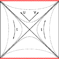
Figure 3: Black hole AdS space in Kruskal coordinates. The $(x,y)$-space, which is attached at each point, is not shown. The boundary (left/right edge) is located at $uv=-1$, the horizon (diagonal lines) is located at $uv=0$ and the singularity (upper/lower edge) is located at $uv=1$. Dashed lines represent surfaces of constant $u$. Time $t$ is flowing upwards in the right wedge and downwards in the left wedge.

Eq.(85) is consistent with the isotropic case of Ref.Blake2016b . The solution can be expressed in terms of the 0th modified Bessel function of the second kind $\mathcal{K}_{0}$ as

$$h(x,y)\propto-\frac{b\,c_{x}c_{y}}{2\pi}\mathcal{K}_{0}(m_{h}\varrho),$$ (87)

where $\varrho^{2}={c_{x}^{2}x^{2}+c_{y}^{2}y^{2}}$. At large values of $\varrho$, i.e. at large spatial distances, this gives

$$h(x,y)\propto\frac{1}{{\sqrt{\varrho}}}\exp\left[{2\pi T\left({t_{w}-\frac{m_{h}}{2\pi T}\varrho}\right)}\right].$$ (88)

From the exponent we can extract the direction-averaged scale for the velocity

$$\bar{v}_{\mathrm{B}}=\frac{2\pi T}{m_{h}}.$$ (89)

In order to switch to the original system of coordinates, we use the identity $uv\,g_{uv}(uv)=g_{tt}(r)/\partial_{r}g_{tt}(r_{+})^{2}$ and obtain

$$\bar{v}_{\mathrm{B}}^{2}=-{\frac{2\pi TL}{d_{\text{eff}}-\theta}}r_{+}^{\theta-z}.$$ (90)

To determine the butterfly velocity along $x$, we consider the case where $y=0$ and we move in the $x$-direction. This gives

$$\frac{\varrho}{\bar{v}_{\mathrm{B}}}=\frac{c_{x}|x|}{\bar{v}_{\mathrm{B}}}\equiv\frac{|x|}{v_{\mathrm{B},x}}.$$ (91)

It then follows for the velocity along the $\alpha$-direction

$$v_{\mathrm{B},\alpha}=\frac{\bar{v}_{\mathrm{B}}}{\sqrt{g_{\alpha\alpha}(r_{+})}},$$ (92)

in accord with Ref.Jeong2018 ; Pedraza2018 ; 1805.01470 ; 1610.02669 ; 1710.05765 ; Blake:2017qgd . This result violates the upper bound of the isotropic case pointed out in Ref.1612.00082 , consistently with Ref.1708.07243 ; 1811.06949

Considering the ratio between the diffusion constant (82) and the square butterfly velocity we finally obtain

$$\frac{D_{\text{c},\alpha}}{v_{\text{B},\alpha}^{2}}=\frac{d_{\text{eff}}-\theta}{\Delta_{\chi}}\frac{1}{2\pi T},$$ (93)

which yields the result Eq.(8) for the diffusivity bound.

5 Conclusions

Motivated by previous results in anisotropic Dirac systems Link2018 , in this paper we analyzed transport coefficients at a quantum Lifshitz point in the strong coupling limit, using scaling arguments and exploiting the duality between quantum field theories and gravity theories. We have focused on particle-hole symmetric theories at charge neutrality which admit a gravitational dual description. We have shown that bounds on transport coefficients of the isotropic case can be generalized to the anisotropic one.
We analyzed the behavior of several observables after a spacetime dilatation, emphasizing that the scale dimensionless ones must approach a constant value for low temperatures. It turned out that some elements of the $\eta/s$-tensor have a nonzero dimension while the diffusivity still exhibits the scaling of the rotational invariant case. In order to address the former, we included the electric transport, multiplying the ratio by a specific combination of conductivities such that the dimension of the resulting quantity is zero.
Within the Einstein-Maxwell-dilaton model considered, translational symmetry is broken along the $y$ direction by a massless scalar in the bulk with a bulk profile linear in $y$. Thus, the $x$-component of the momentum is still conserved and $T_{\alpha x}$ continues to be the current of a conserved quantity. Therefore, the viscosity tensor elements $\eta_{\alpha x\beta x}$ maintain their meaning as hydrodynamic transport coefficients. Since we can find solutions of the field equations that yield either $\phi<1$ or $\phi>1$, we can always construct an anisotropic geometry that violates the isotropic viscosity bound for at least one tensor element, while fulfilling the generalized bound given in Eq.(7).

In the direction where translations are broken, momentum relaxes at a rate $1/\tau_{\text{mr}}$. In a holographic system with slow momentum relaxation $1/\tau_{\text{mr}}\ll\Lambda$, where $\Lambda$ is a UV cutoff, there is a range of intermediate times $1/\tau_{\text{mr}}\lesssim t\ll\Lambda$ where momentum is approximately conserved. In this regime, the viscosity can be defined from the shear Kubo formula, yet is still found to violate the viscosity-to-entropy-density-ratio bound. Alternatively, it is likely that the diffusivity of transverse momentum is a better quantity to bound: the results of Ref.Ciobanu:2017fef show that it obeys a bound of the kind (2), with the speed of light as the characteristic velocity.

We also discussed the effects of translational symmetry breaking on the conductivity-viscosity bound, both in the explicit and spontaneous setups. In this latter case, deviations from the bound are more suppressed for high enough temperatures than in the explicit one.

Differently from the other quantities, the diffusivity is not solely given by data on the horizon and is expressed through an integral over the radial direction. Although we do not have the full expression of bulk fields, we have derived a near horizon formula for the compressibility, and could relate the diffusion constant to the horizon data in a simple fashion. Indeed, the near IR geometry dominates at low temperature Blake2016 ; Davison:2018ofp ; Davison2018 . On the other hand we have calculated the butterfly velocities by moving to the Kruskal system of coordinates and using a generalization of the shock-wave technique. We have computed the proportionality factor between the diffusivity to the square butterfly velocity ratio and the inverse temperature, finding that it can be expressed in terms of the critical exponents $z,\phi$, and $\theta$.
It is well-known that the KSS bound can be violated by terms containing more than two derivatives of the metric (see Ref.Cremonini:2011iq for a review), which capture finite ’t Hooft coupling corrections. A possible extension of our work would be to consider the effects of higher derivative terms involving the massless scalars, along the lines of Ref.Baggioli2017 . Moreover, particle-hole symmetry breaking could be taken into account as well.
In our work, the anisotropy was sourced by a massless scalar that also breaks translations. As we have discussed, only the bound involving the transverse viscosity is preserved. In Ref.1604.01346 , isotropy is broken by one of the spatial components of the gauge field acquiring a vev. In this setup, translations are unbroken and viscosities are still well-defined hydrodynamic transport coefficients. Their results, specifically equation (14), show that the bound (6) holds in this holographic setup. It would be interesting to further investigate such systems, as well as different sources of spontaneous anisotropy, Donos:2012gg ; Hoyos:2020zeg .
Thus, we conclude that the transport properties of a strongly-interacting many-body system near a quantum Lifshitz point can be efficiently described using holographic methods and requires a generalization of the viscosity bound obtained in isotropic theories.

Appendix A Scaling of the viscosity tensor

In this appendix we offer an alternative derivation of the scaling dimension, Eq.(25) of the viscosity tensor. The analysis leads to results identical to those presented in Section 2 of the paper.
Since the viscosity tensor describes the linear response to the temporal change of an externally-applied strain field, we can also define it using the strain generators $\mathcal{J}_{\alpha\beta}.$ The strain generators describe the deformation of the coordinate systems due to an applied external strain and are given by Bradlyn2012 ; Link2018b $\mathcal{J}_{\alpha\beta}=x_{\alpha}k_{\beta}+\frac{i}{2}\delta_{\alpha\beta}$. Hence, the viscosity tensor is defined as

$$\eta_{\alpha\beta\gamma\delta}(\omega)=\omega\,\mathrm{Im}\chi_{\alpha\beta\gamma\delta}^{(\mathcal{J})}(\omega)\,,$$ (94)

with $\chi_{\alpha\beta\gamma\delta}^{(\mathcal{J})}(\omega)$ being the Fourier transform of $\chi^{\mathcal{J}}_{\alpha\beta\gamma\delta}(t)=-i\theta(t)\langle[J_{\alpha\beta}(t),J_{\gamma\delta}(0)]\rangle$, where $J_{\alpha\beta}$ is the density of the strain generator $\mathcal{J}_{\alpha\beta}$. In order to obtain the scaling dimension of the correlation function, we assume for the strain generator density the same dimensionality as the particle density $\Delta_{\rho}=d_{eff}$ times the scaling dimension of the momentum coordinates $k_{\beta}$ , $k_{\delta}$ and the spatial coordinates $x_{\alpha}$, $x_{\gamma}$, which have the dimensionality of the inverse momentum. We find for the correlation function of the two strain generators

$$\chi_{\alpha\beta\gamma\delta}^{(\mathcal{J})}(k_{\perp},\boldsymbol{k}_{\parallel},\omega)=b^{-\Delta_{\mathcal{J},\alpha\beta\gamma\delta}}\chi_{\alpha\beta\gamma\delta}^{(\mathcal{J})}(b^{\phi}k_{\perp},b\boldsymbol{k}_{\parallel},b^{z}\omega)$$ (95)

with $\Delta_{\mathcal{J},\alpha\beta\gamma\delta}=d_{\mathrm{eff}}-z-\varphi_{\alpha}+\varphi_{\beta}-\varphi_{\gamma}+\varphi_{\delta}.$ Here we used the same notation as in the main paper, where $\varphi_{\alpha}=1$ if the $\alpha$-component is alinged along the direction of $\boldsymbol{k}_{\parallel}$ and $\varphi_{\alpha}=\phi$ for the direction of $k_{\perp}$. Using $\Delta_{\mathcal{J},\alpha\beta\gamma\delta}$ allows us to determine the scaling behavior of the viscosity tensor

$$\eta_{\alpha\beta\gamma\delta}(T,\omega)=b^{-\Delta_{\eta,\alpha\beta\gamma\delta}}\eta_{\alpha\beta\gamma\delta}(b^{z}T,b^{z}\omega)$$ (96)

with

$$\Delta_{\eta,\alpha\beta\gamma\delta} = \Delta_{\mathcal{J},\alpha\beta\gamma\delta}+z$$ (97)

$$= d_{\mathrm{eff}}-\varphi_{\alpha}+\varphi_{\beta}-\varphi_{\gamma}+\varphi_{\delta}\>,$$

which is in agreement with Eq.(25) of the main part of the paper.

Appendix B IR models

In order to analyze the IR metric (45), we derive the hyperscaling-violating solutions in the presence of both one and two massless scalar fields. It is worth to emphasize that the radial coordinate parameterizing the IR geometry (45) does not coincide with the one in the UV region (42). Davison2018 To be specific, we consider the matter Lagrangian

$${\cal L}_{\text{M}}=-\frac{1}{2}\left(\nabla\varphi\right)^{2}+V_{0}r^{2\kappa\delta}-\sum_{\alpha=1}^{p}\frac{r^{2\kappa\lambda_{\alpha}}}{2}\left(\nabla\psi_{\alpha}\right)^{2}-\frac{r^{2\kappa\zeta}}{4}F^{2},$$ (98)

where $p$ is the number of massless scalars and $\psi_{\alpha}=a_{\alpha}x_{\alpha}$, with no index summation. In the $p=1$ case it reduces to (35).
The effective dilaton potential (40) looks like

$$\frac{V_{\text{eff}}(r)}{\sqrt{-g}}=\frac{1}{2}\sum_{\alpha=1}^{p}a_{\alpha}^{2}r^{2\Lambda_{\alpha}-\theta}-V_{0}r^{2\delta\kappa},$$ (99)

where $\Lambda_{1}=\kappa\lambda_{x}+\phi$ and $\Lambda_{2}=\kappa\lambda_{y}+1$.

B.1 Marginally relevant case

In order to avoid radial dependences coming from the $a_{\alpha}$-terms, we set $2\Lambda_{\alpha}=2\kappa\delta+\theta$. This corresponds to take the massless scalars as marginal deformations of the IR fixed point. Furthermore, setting $\theta+2\delta\kappa=0$ yields a set of algebraic equations in both the cases $p=1,2$.
Let us start with the one single massless scalar case $p=1$ – we omit the subscript $\alpha=1$ everywhere. The solution to the field equations is given by:

$$z=\phi,\quad 2\kappa\delta=-\theta,\quad\kappa\lambda=-1,$$

$$4\kappa^{2}=\theta^{2}-2\theta\phi+2\phi-2,$$

$$L^{2}={(\theta-2\phi-1)(\theta-2\phi)}/{V_{0}},$$

$$a^{2}=\frac{2V_{0}(1-\phi)}{\theta-2\phi}.$$ (100)

Note how a low momentum dissipation limit ($a\to 0$) always restores the isotropy of the system ($\phi=1$). In order to get a realistic solution, we demand the positivity of the squared quantities and the specific heat $c=T\,\partial_{T}s$. In addition, we require the vanishing of the line element in the IR at $T=0$, obtaining the following set of conditions:

$$\theta<2,\,\,\,\theta^{2}+2\phi>2\theta\phi+2,\,\,\,\phi>1,$$ (101)

$$\theta>2,\,\,\,\theta^{2}+2\phi>2\theta\phi+2,\,\,\,\theta\phi<\phi^{2}+\phi.$$ (102)

In the former the IR is at $r=\infty$, in the latter at $r=0$. The null energy condition (NEC) turns out to be fulfilled.

In the $p=2$ case we find

$$2\kappa\delta=-\theta,\quad\kappa\lambda_{x}=-\phi,\quad\kappa\lambda_{y}=-1,$$

$$4\kappa^{2}=\theta(\theta-2z)-2\phi(\phi-z)-2(1-z),$$

$$L^{2}={(\theta-2z)(\theta-\phi-z-1)}/{V_{0}},$$

$$a_{x}^{2}=\frac{2V_{0}(\phi-z)}{\theta-2z},\quad a_{y}^{2}=\frac{2V_{0}(1-z)}{\theta-2z},$$ (103)

which reproduces Eq.(100) in the $a_{x}=0$ case. The consistency conditions follows from analogue considerations and are depicted in Fig.4 – the NEC is automatically satisfied.

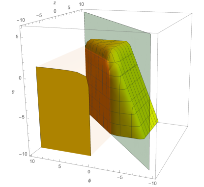
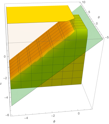
Figure 4: Parameter space for the double marginal massless scalars solution. The intersection with the plane $z=\phi$ coincides with (102).

Even in this case, sending the momentum dissipation to zero restores the isotropy of the system.
One can easily check that the above solution reproduces the single massless scalar one when $a_{x}=0$.

B.2 Irrelevant case

Now we wish to investigate the $p=1$ case, where the massless scalar acts as an irrelevant deformation of the IR endpoint. Details on the $p=2$ mixed case can be found in Ref.Davison2018 ; Jeong2018 . We firstly determine the solution when $a=0$ and then consider perturbations of the form:

$$\Phi=\Phi_{a=0}\left(1+c_{\Phi}a^{2}r^{2\Delta_{a}}\right).$$ (104)

$\Phi$ stands for the metric elements or the dilaton field, and $c_{\Phi}$ are numerical coefficients that follow from the $\mathcal{O}(a^{2})$ fields equations. Such corrections are expressed in terms of $a^{2}$ as the massless scalar enters quadratically the field equations. The leading solution is given by

$$z=\phi=1,$$

$$4\kappa^{2}=\theta(\theta-2),$$

$$L^{2}={(\theta-2)(\theta-3)}/{V_{0}},$$ (105)

provided that $\theta+2\delta\kappa=0$. Moreover we obtain

$$\Delta_{a}=1+\kappa\lambda$$ (106)

in accord with Ref.Davison2018 . The consistency conditions read

$$\theta<0,\quad\Delta_{a}<0,$$ (107)

given that the IR is located at $r\to+\infty$.

Appendix C The holographic dual of out-of-time-order correlation functions

In the context of the butterfly velocity, we consider out-of-time-order correlation functions (OTOCs) of the form $C(\vec{x},t_{w})=-\langle[A(\vec{x},t_{w}),B(0,0)]^{2}\rangle$, where $A$ and $B$ are hermitian local operators. In order to translate such functions to the holographic language, it is convenient to regularize them by rotating one of the commutators halfway around the thermal circle Maldacena2016 . This results in

$$C(\vec{x},t_{w})=-\mathrm{tr}\left[\bar{y}[A(\vec{x},t_{w}),B(0,0)]\bar{y}[A(\vec{x},t_{w}),B(0,0)\right],$$ (108)

where $\bar{y}$ is the squareroot of the density matrix. Next, we introduce the thermofield-double (TFD) state

$$\ket{\beta}=\frac{1}{\mathcal{Z}^{1/2}}\sum_{n}e^{-\beta E_{n}/2}\ket{n}_{\mathrm{L}}\!\ket{n}_{\mathrm{R}},$$ (109)

with the partition function $\mathcal{Z}$ and the inverse temperature $\beta$. This state lies in the product space of two copies of the Hilbert space and $\ket{n}_{\mathrm{L}}$ and $\ket{n}_{\mathrm{R}}$ denote energy Eigenstates with Eigenvalues $E_{n}$ in the respective copies. Operators acting on the two copies are defined as $O_{\mathrm{L}}=O^{\top}\otimes{\mathbb{1}}$ and $O_{\mathrm{R}}={\mathbb{1}}\otimes O$. With these definitions, the regularized OTOC can be written as an expectation value in the TFD state, i.e.

$$C(\vec{x},t_{w})=-\bra{\beta}[B_{\mathrm{L}}(0,0),A_{\mathrm{L}}(\vec{x},t_{w})]\cdot[A_{\mathrm{R}}(\vec{x},t_{w}),B_{\mathrm{R}}(0,0)]\!\ket{\beta}.$$ (110)

Furthermore, we note that the TFD state is invariant under time translations generated by $H_{\mathrm{tot}}=H_{\mathrm{R}}-H_{\mathrm{L}}$.

To proceed, we need to investigate the transition amplitudes prepared by $\ket{\beta}$ in order to identify the spacetime connecting the L and the R system. For two given states $\ket{\xi}$ and $\ket{\zeta}$, these transition amplitudes are given by

$$\bra{\xi}_{\mathrm{R}}\!\braket{\zeta}{{}_{\mathrm{L}}}{\beta}\propto\braket{\zeta}{e^{-\beta H/2}}{\tilde{\xi}},$$ (111)

where the conjugate state $\ket{\tilde{\xi}}$ is defined such that $\braket{n}{\tilde{\xi}}=\braket{\xi}{n}$ for all states $\ket{n}$. This definition is only well-defined if the states $\ket{n}$ are redefined by $\ket{n}\to e^{-i\mathrm{arg}\braket{\xi}{n}}\ket{n}$ in order to make the scalar products real. Using the fact that the Hamilton operator $H$ is obtained from the Hamilton density by integrating over the position space $\mathcal{P}$, the transition amplitude shows that the L and R systems are connected by the spacetime

$$\mathcal{B}=[0,\beta/2]\times\mathcal{P}.$$ (112)

According to the holographic dictionary, this spacetime is the boundary of its holographic dual. It was shown in Maldacena2001 , that the holographic dual of the TFD state is given by a two-sided black hole spacetime. For simplicity, we will demonstrate this for the case of a one-dimensional position space $\mathcal{P}$, but the results hold in any dimension. We first consider a Euclidean black hole in three dimensions, whose metric can be written in the two equivalent forms

$$ds^{2} =(r^{2}-r_{+}^{2})d\tau^{2}+\frac{1}{r^{2}-r_{+}^{2}}dr^{2}+g_{xx}(r)dx^{2},$$ (113)

$$ds^{2} =\frac{4}{(1-zz^{\star})^{2}}dzdz^{\star}+g_{xx}(zz^{\star})dx^{2}.$$ (114)

The coordinate $x$ is restricted to the position space $\mathcal{P}$ and the two expressions are related by $z=e^{\frac{2\pi}{\beta}(r_{\star}(r)-i\tau)}$ with the tortoise coordinate. Here, $g_{tt}(r)=g_{\tau\tau}(r)=r^{2}-r_{+}^{2}$ and $g_{rr}(r)=1/(r^{2}-r_{+}^{2})$.

If $\tau$ is restricted to the Euclidean time interval $[0,\beta/2]$, the boundary of the Euclidean black hole is equal to $\mathcal{B}$. This can be achieved by cutting the spacetime along the $\mathrm{Im}(z)=0$ surface. Furthermore, the metric is invariant under time translations of the form $z\to z\cdot e^{-i\frac{2\pi}{\beta}\Delta\tau}$. Such time translations change the position of the $\mathrm{Im}(z)=0$ surface, but leave the distance between its two boundary points invariant.

What remains to be implemented, is the Lorentzian time invariance. We achieve this analytic continuation by introducing Kruskal coordinates $z=-v$ and $z^{\star}=u$, yielding

$$ds^{2}=\frac{-4}{(1+uv)^{2}}dudv+g_{xx}(uv)dx^{2}.$$ (115)

This metric is invariant under Lorentzian time translations $u\to u\cdot e^{-\frac{2\pi}{\beta}\Delta t}$, $v\to v\cdot e^{\frac{2\pi}{\beta}\Delta t}$. In order to continuously connect the Kruskal coordinate frame to the Euclidean black hole, we rewrite $u=t+w$ and $v=t-w$, giving

$$ds^{2}=\,\frac{-4}{(1+t^{2}-w^{2})^{2}}dt^{2}+\frac{4}{(1+t^{2}-w^{2})^{2}}dw^{2}+g_{xx}(uv)dx^{2}.$$ (116)

At $t=0$, this metric is equal to the Euclidean black hole at the $\mathrm{Im}(z)=0$ surface. Thus, we can glue the Kruskal extension of the Lorentzian black hole to the Euclidean black hole along these surfaces (see Fig.5). The resulting spacetime is the holographic dual of the TFD state.

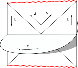
Figure 5: The plane represents the two-sided black hole in Lorentzian time. This is glued to the $\mathrm{Im}(z)=0$ surface of the Euclidean spacetime along the $t=0$ surface. The boundary regions L and R are separated along the thermal circle by a Euclidean time interval of length $\beta/2$. Lorentzian time flows forwards on the right boundary and backwards on the left boundary. The position space, which is attached at each point, is omitted.

Now that we have demonstrated the duality between the TFD state and a two-sided black hole for a one-dimensional $\mathcal{P}$, we can return to a two-dimensional $\mathcal{P}$ and implement the effect of the OTOC. OTOCs are used as a measure for the butterfly effect, which describes how a microscopic effect (on UV energy scales) can become a macroscopic effect (on IR energy scales) at later times. This motivated Shenker and Stanford to propose that the OTOC can be modelled hoographically by a massless particle, which is thrown into the system at the boundary (the UV region) and has an effect at the horizon (the IR region) at a later time Shenker2014 .

In order to quantify the effect of such a particle, we start with the action of a point particle, which can be written in the form

$$\mathcal{S}[z^{\rho}]=\frac{1}{2}\int d\lambda\,e(\lambda)\left(\frac{1}{e(\lambda)^{2}}\frac{dz^{\alpha}}{d\lambda}\frac{dz^{\beta}}{d\lambda}g_{\alpha\beta}(z^{\rho}(\lambda))-m^{2}\right).$$ (117)

Here, $z^{\rho}(\lambda)$ is a geodesic with affine parameter $\lambda$ and $e(\lambda)$ is a non-dynamical auxiliary field called ’Einbein’. In the massive case, this field is entirely fixed by the field equations and in the massless case, it can be interpreted as a gauge degree of freedom. The stress-energy tensor for a massless particle is given by

$$T_{\mu\nu}(x^{\rho})=\frac{2}{\sqrt{-g(x^{\rho})}}\frac{\delta\mathcal{S}}{\delta g^{\mu\nu}}=\int d\lambda\frac{1}{e(\lambda)}\frac{dz_{\mu}}{d\lambda}\frac{dz_{\nu}}{d\lambda}\frac{\delta^{(4)}(x^{\rho}-z^{\rho}(\lambda))}{\sqrt{-g(x^{\rho})}}.\qquad$$ (118)

A light-like infalling geodesic requires $dt/dr=-1/\gamma(r)$. If the particle is inserted at the boundary at time $-t_{w}$ , the resulting geodesic is given by

$$(z^{\mu}(\lambda))^{\top}=(-r_{\star}(\bar{r}(\lambda))-t_{w},\bar{r}(\lambda),0,0),$$ (119)

where $\bar{r}(\lambda)$ denotes the radial coordinate at position $\lambda$. If $\lambda$ is identified with the radial coordinate, $e(\lambda)$ has units of inverse mass and can be identified as the inverse of the particle energy $E$. Such a parameterization may not in general be a solution of the geodesic equation. However, for a different parameterization, the resulting stress-energy tensor would only change by a global factor. It is thus sufficient to assume the $\bar{r}(\lambda)=\lambda$ case.

The stress-energy tensor is now given by

$$T^{\mu\nu}(x^{\rho})=E\frac{\delta(x)\delta(y)\delta(t+t_{w}+r_{\star}(r))}{\sqrt{-g(x^{\rho})}}\cdot\left(\frac{\delta^{\mu t}\delta^{\nu t}}{\gamma^{2}(r)}-\frac{\delta^{\mu t}\delta^{\nu r}+\delta^{\mu r}\delta^{\nu t}}{\gamma(r)}+\delta^{\mu r}\delta^{\nu r}\right).$$ (120)

At large $t_{w}$, after switching to Kruskal coordinates, the only non-vanishing component of the stress-energy tensor for a particle inserted at the right boundary is given by

$$T_{vv}\propto Ee^{\frac{2\pi}{\beta}t_{w}}\delta(x)\delta(y)\delta(v).$$ (121)

For a particle inserted at the left boundary, time is reversed ($t\leftrightarrow-t$), which is equivalent to $u\leftrightarrow v$. In this case, the stress-energy tensor is given by

$$T_{uu}\propto Ee^{\frac{2\pi}{\beta}t_{w}}\delta(x)\delta(y)\delta(u).$$ (122)

As discussed above, perturbing a two-sided black hole with this stress-energy tensor results in a shock wave, which can be identified as the OTOC.

References

- (1) P. K. Kovtun, D. T. Son and A. O. Starinets, Viscosity in strongly interacting quantum field theories from black hole physics, Phys. Rev. Lett. 94 (Mar, 2005) 111601.
- (2) T. Schäfer, Fluid dynamics and viscosity in strongly correlated fluids, Annual Review of Nuclear and Particle Science 64 (2014) 125–148, [arXiv:1403.0653].
- (3) J. Thomas, Is an ultra-cold strongly interacting fermi gas a perfect fluid?, Nuclear Physics A 830 (2009) 665c – 672c, [arXiv:0907.0140].
- (4) M. Müller, J. Schmalian and L. Fritz, Graphene: A nearly perfect fluid, Phys. Rev. Lett. 103 (Jul, 2009) 025301, [arXiv:0903.4178].
- (5) J. M. Maldacena, The Large N limit of superconformal field theories and supergravity, Int. J. Theor. Phys. 38 (1999) 1113–1133, [hep-th/9711200].
- (6) E. Witten, Anti-de Sitter space, thermal phase transition, and confinement in gauge theories, Adv. Theor. Math. Phys. 2 (1998) 505–532, [hep-th/9803131].
- (7) S. Gubser, I. Klebanov and A. Polyakov, Gauge theory correlators from non-critical string theory, Physics Letters B 428 (1998) 105 – 114.
- (8) A. F. Ioffe and A. R. Regel, Non-crystalline, amorphous and liquid electronic semiconductors, Prog. Semicond. 26 (1960) 237–291.
- (9) N. F. Mott, Conduction in non-crystalline systems ix. the minimum metallic conductivity, The Philosophical Magazine: A Journal of Theoretical Experimental and Applied Physics 26 (1972) 1015–1026, [https://doi.org/10.1080/14786437208226973].
- (10) M. Gurvitch, Ioffe-regel criterion and resistivity of metals, Phys. Rev. B 24 (Dec, 1981) 7404–7407.
- (11) V. J. Emery and S. A. Kivelson, Superconductivity in bad metals, Phys. Rev. Lett. 74 (Apr, 1995) 3253–3256.
- (12) N. E. Hussey, K. Takenaka and H. Takagi, Universality of the mott–ioffe–regel limit in metals, Philosophical Magazine 84 (2004) 2847–2864, [https://doi.org/10.1080/14786430410001716944].
- (13) J. Zaanen, Why the temperature is high, Nature 430 (2004) 512–513.
- (14) S. Sachdev, Quantum Phase Transitions. Cambridge University Press, 2 ed., 2011, 10.1017/CBO9780511973765.
- (15) S. A. Hartnoll, Theory of universal incoherent metallic transport, Nature Physics 11 (Dec, 2014) 54 EP –, [arXiv:1405.3651].
- (16) M. Blake, Universal charge diffusion and the butterfly effect in holographic theories, Phys. Rev. Lett. 117 (Aug, 2016) 091601.
- (17) M. Blake, Universal diffusion in incoherent black holes, Phys. Rev. D 94 (Oct, 2016) 086014, [arXiv:1604.01754].
- (18) S. H. Shenker and D. Stanford, Black holes and the butterfly effect, Journal of High Energy Physics 2014 (Mar, 2014) 67, [arXiv:1306.0622].
- (19) S. H. Shenker and D. Stanford, Stringy effects in scrambling, Journal of High Energy Physics 2015 (May, 2015) 132, [arXiv:1412.6087].
- (20) D. A. Roberts, D. Stanford and L. Susskind, Localized shocks, Journal of High Energy Physics 2015 (Mar, 2015) 51, [arXiv:1409.8180].
- (21) D. A. Roberts and B. Swingle, Lieb-robinson bound and the butterfly effect in quantum field theories, Phys. Rev. Lett. 117 (Aug, 2016) 091602.
- (22) J. Maldacena, S. H. Shenker and D. Stanford, A bound on chaos, Journal of High Energy Physics 2016 (Aug, 2016) 106, [arXiv:1503.01409].
- (23) M. Blake, R. A. Davison and S. Sachdev, Thermal diffusivity and chaos in metals without quasiparticles, Phys. Rev. D96 (2017) 106008, [arXiv:1705.07896].
- (24) M. J. Klug, M. S. Scheurer and J. Schmalian, Hierarchy of information scrambling, thermalization, and hydrodynamic flow in graphene, Phys. Rev. B 98 (Jul, 2018) 045102, [arXiv:1712.08813].
- (25) R. A. Davison, S. A. Gentle and B. Goutéraux, Slow relaxation and diffusion in holographic quantum critical phases, arXiv:1808.05659.
- (26) R. A. Davison, S. A. Gentle and B. Goutéraux, Impact of irrelevant deformations on thermodynamics and transport in holographic quantum critical states, arXiv:1812.11060.
- (27) S. Grozdanov, K. Schalm and V. Scopelliti, Black hole scrambling from hydrodynamics, arXiv:1710.00921.
- (28) T. Hartman, S. A. Hartnoll and R. Mahajan, An upper bound on transport, arXiv:1706.00019.
- (29) R. A. Davison and B. Goutéraux, Momentum dissipation and effective theories of coherent and incoherent transport, JHEP 01 (2015) 039, [arXiv:1411.1062].
- (30) S. Grozdanov, A. Lucas and N. Poovuttikul, Holography and hydrodynamics with weakly broken symmetries, Phys. Rev. D99 (2019) 086012, [arXiv:1810.10016].
- (31) C. Q. Cook and A. Lucas, Electron hydrodynamics with a polygonal fermi surface, Phys. Rev. B 99 (Jun, 2019) 235148, [arXiv:1903.05652].
- (32) J. M. Link, B. N. Narozhny, E. I. Kiselev and J. Schmalian, Out-of-bounds hydrodynamics in anisotropic dirac fluids, Phys. Rev. Lett. 120 (May, 2018) 196801, [arXiv:1708.02759].
- (33) E. M. Lifshitz, On the theory of phase transformations of the second order. i. changes of the elementary cell of a crystal in phase transitions of the second order., J. Phys. (Moscow) 6 (1942) 61–74.
- (34) I. E. Dzyaloshinski, Theory of helicoidal structures in antiferromagnets. i. nonmetals, Sov. Phys. JETP 19 (1964) 960.
- (35) S. Goshen, D. Mukamel and S. Shtrikman, Non-crystalline, amorphous and liquid electronic semiconductors, Int. J. Magn. 6 (1974) 221.
- (36) R. M. Hornreich, M. Luban and S. Shtrikman, Critical behavior at the onset of -space instability on the line, Phys. Rev. Lett. 35 (Dec, 1975) 1678–1681.
- (37) H. W. Diehl and M. Shpot, Critical behavior at m-axial lifshitz points: Field-theory analysis and -expansion results, Phys. Rev. B 62 (Nov, 2000) 12338–12349.
- (38) M. Shpot and H. Diehl, Two-loop renormalization-group analysis of critical behavior at m-axial lifshitz points, Nuclear Physics B 612 (2001) 340 – 372.
- (39) M. A. Shpot, Y. M. Pis’mak and H. W. Diehl, Large-n expansion form-axial lifshitz points, Journal of Physics: Condensed Matter 17 (may, 2005) S1947–S1972.
- (40) M. A. Shpot, H. W. Diehl and Y. M. Pis’mak, Compatibility of 1/n and epsilon expansions for critical exponents at m-axial lifshitz points, arXiv:0802.2434.
- (41) A. Rebhan and D. Steineder, Violation of the holographic viscosity bound in a strongly coupled anisotropic plasma, Phys. Rev. Lett. 108 (Jan, 2012) 021601, [arXiv:1110.6825].
- (42) S. Jain, R. Samanta and S. P. Trivedi, The shear viscosity in anisotropic phases, Journal of High Energy Physics 2015 (Oct, 2015) 28, [arXiv:1506.01899].
- (43) X.-H. Ge, Y. Ling, C. Niu and S.-J. Sin, Thermoelectric conductivities, shear viscosity, and stability in an anisotropic linear axion model, Phys. Rev. D92 (2015) 106005, [arXiv:1412.8346].
- (44) X.-H. Ge, S.-J. Sin and S.-F. Wu, Universality of dc electrical conductivity from holography, arXiv:1512.01917.
- (45) M. Baggioli, B. Padhi, P. W. Phillips and C. Setty, Conjecture on the butterfly velocity across a quantum phase transition, arXiv:1805.01470.
- (46) K. A. Mamo, Holographic rg flow of the shear viscosity to entropy density ratio in strongly coupled anisotropic plasma, arXiv:1205.1797.
- (47) D. Giataganas, Observables in strongly coupled anisotropic theories, arXiv:1306.1404.
- (48) D. Giataganas, U. Gürsoy and J. F. Pedraza, Strongly coupled anisotropic gauge theories and holography, Phys. Rev. Lett. 121 (Sep, 2018) 121601, [arXiv:1708.05691].
- (49) H. Isobe, B.-J. Yang, A. Chubukov, J. Schmalian and N. Nagaosa, Emergent non-fermi-liquid at the quantum critical point of a topological phase transition in two dimensions, Phys. Rev. Lett. 116 (Feb, 2016) 076803, [arXiv:1508.03781].
- (50) A. Kobayashi, Y. Suzumura, F. Piéchon and G. Montambaux, Emergence of dirac electron pair in the charge-ordered state of the organic conductor -(bedt-ttf)2i3, Phys. Rev. B 84 (Aug, 2011) 075450, [arXiv:1107.4841].
- (51) V. Pardo and W. E. Pickett, Half-metallic semi-dirac-point generated by quantum confinement in nanostructures, Phys. Rev. Lett. 102 (Apr, 2009) 166803.
- (52) S. Banerjee, R. R. P. Singh, V. Pardo and W. E. Pickett, Tight-binding modeling and low-energy behavior of the semi-dirac point, Phys. Rev. Lett. 103 (Jul, 2009) 016402, [arXiv:0906.1564].
- (53) C. Fang and L. Fu, New classes of three-dimensional topological crystalline insulators: Nonsymmorphic and magnetic, Phys. Rev. B 91 (Apr, 2015) 161105.
- (54) S.-M. Huang, S.-Y. Xu, I. Belopolski, C.-C. Lee, G. Chang, T.-R. Chang et al., A new type of weyl semimetal with quadratic double weyl fermions in srsi2, Proceedings of the National Academy of Sciences 113 (2016) 1180–1185, [arXiv:1503.05868].
- (55) H.-S. Jeong, Y. Ahn, D. Ahn, C. Niu, W.-J. Li and K.-Y. Kim, Thermal diffusivity and butterfly velocity in anisotropic q-lattice models, Journal of High Energy Physics 2018 (Jan, 2018) 140, [arXiv:1708.08822].
- (56) A. Donos and J. P. Gauntlett, Novel metals and insulators from holography, JHEP 06 (2014) 007, [arXiv:1401.5077].
- (57) D. Mateos and D. Trancanelli, The anisotropic N=4 super Yang-Mills plasma and its instabilities, Phys. Rev. Lett. 107 (2011) 101601, [arXiv:1105.3472].
- (58) D. Mateos and D. Trancanelli, Thermodynamics and Instabilities of a Strongly Coupled Anisotropic Plasma, JHEP 07 (2011) 054, [arXiv:1106.1637].
- (59) A. Donos and J. P. Gauntlett, Thermoelectric dc conductivities from black hole horizons, Journal of High Energy Physics 2014 (Nov, 2014) 81, [arXiv:1406.4742].
- (60) D. Giataganas, Probing strongly coupled anisotropic plasma, arXiv:1202.4436.
- (61) S. A. Hartnoll, D. M. Ramirez and J. E. Santos, Entropy production, viscosity bounds and bumpy black holes, Journal of High Energy Physics 2016 (Mar, 2016) 170, [arXiv:1601.02757].
- (62) L. Alberte, M. Baggioli and O. Pujolas, Viscosity bound violation in holographic solids and the viscoelastic response, JHEP 07 (2016) 074, [arXiv:1601.03384].
- (63) T. Ciobanu and D. M. Ramirez, Shear hydrodynamics, momentum relaxation, and the KSS bound, arXiv:1708.04997.
- (64) P. Burikham and N. Poovuttikul, Shear viscosity in holography and effective theory of transport without translational symmetry, Phys. Rev. D 94 (Nov, 2016) 106001, [arXiv:1601.04624].
- (65) Y. Ling, Z. Xian and Z. Zhou, Holographic shear viscosity in hyperscaling violating theories without translational invariance, Journal of High Energy Physics 2016 (2016) , [arXiv:1605.03879].
- (66) Y. Ling, Z. Xian and Z. Zhou, Power Law of Shear Viscosity in Einstein-Maxwell-Dilaton-Axion model, Chin. Phys. C41 (2017) 023104, [arXiv:1610.08823].
- (67) X.-H. Ge, Notes on shear viscosity bound violation in anisotropic models, arXiv:1510.06861.
- (68) A. Amoretti, D. Areán, B. Goutéraux and D. Musso, Effective holographic theory of charge density waves, Phys. Rev. D97 (2018) 086017, [arXiv:1711.06610].
- (69) A. Amoretti, D. Areán, B. Goutéraux and D. Musso, DC resistivity of quantum critical, charge density wave states from gauge-gravity duality, Phys. Rev. Lett. 120 (2018) 171603, [1712.07994].
- (70) A. Amoretti, D. Areán, B. Goutéraux and D. Musso, Diffusion and universal relaxation of holographic phonons, JHEP 10 (2019) 068, [1904.11445].
- (71) Y. Ling, P. Liu and J.-P. Wu, Holographic butterfly effect at quantum critical points, arXiv:1610.02669.
- (72) W.-H. Huang, Holographic butterfly velocities in brane geometry and einstein-gauss-bonnet gravity with matters, arXiv:1710.05765.
- (73) V. Jahnke, Delocalizing entanglement of anisotropic black branes, arXiv:1708.07243.
- (74) V. Jahnke, Recent developments in the holographic description of quantum chaos, arXiv:1811.06949.
- (75) L. Huijse, S. Sachdev and B. Swingle, Hidden Fermi surfaces in compressible states of gauge-gravity duality, Phys. Rev. B85 (2012) 035121, [arXiv:1112.0573].
- (76) R. Shankar, Renormalization-group approach to interacting fermions, Rev. Mod. Phys. 66 (Jan, 1994) 129–192.
- (77) B. Goutéraux, Charge transport in holography with momentum dissipation, JHEP 04 (2014) 181, [arXiv:1401.5436].
- (78) S. A. Hartnoll and A. Karch, Scaling theory of the cuprate strange metals, Phys. Rev. B91 (2015) 155126, [arXiv:1501.03165].
- (79) J. M. Link, D. E. Sheehy, B. N. Narozhny and J. Schmalian, Elastic response of the electron fluid in intrinsic graphene: The collisionless regime, Phys. Rev. B 98 (Nov, 2018) 195103, [arXiv:1808.04658].
- (80) B. Bradlyn, M. Goldstein and N. Read, Kubo formulas for viscosity: Hall viscosity, ward identities, and the relation with conductivity, Phys. Rev. B 86 (Dec, 2012) 245309, [arXiv:1207.7021].
- (81) K. S. Thorne, R. H. Price and D. A. MacDonald, Black holes: The membrane paradigm. 1986.
- (82) N. Iqbal and H. Liu, Universality of the hydrodynamic limit in ads/cft and the membrane paradigm, Phys. Rev. D 79 (Jan, 2009) 025023, [arXiv:0809.3808].
- (83) S. S. Gubser, I. R. Klebanov and A. M. Polyakov, Gauge theory correlators from noncritical string theory, Phys. Lett. B428 (1998) 105–114, [hep-th/9802109].
- (84) D. T. Son and A. O. Starinets, Minkowski-space correlators in AdS/CFT correspondence: recipe and applications, Journal of High Energy Physics 2002 (sep, 2002) 042–042, [arXiv:math/0205051].
- (85) C. P. Herzog and D. T. Son, Schwinger-keldysh propagators from AdS/CFT correspondence, Journal of High Energy Physics 2003 (mar, 2003) 046–046.
- (86) D. Giataganas and H. Soltanpanahi, Universal properties of the langevin diffusion coefficients, arXiv:1310.6725.
- (87) A. Donos and J. P. Gauntlett, Holographic Q-lattices, JHEP 04 (2014) 040, [arXiv:1311.3292].
- (88) T. Andrade and B. Withers, A simple holographic model of momentum relaxation, Journal of High Energy Physics 2014 (May, 2014) 101, [arXiv:1311.5157].
- (89) A. Amoretti, M. Baggioli, N. Magnoli and D. Musso, Chasing the cuprates with dilatonic dyons, Journal of High Energy Physics 2016 (Jun, 2016) 113, [arXiv:1603.03029].
- (90) J. McGreevy, Holographic duality with a view toward many-body physics, Advances in High Energy Physics 2010 (2010) , [arXiv:0909.0518].
- (91) C. Charmousis, B. Goutéraux, B. S. Kim, E. Kiritsis and R. Meyer, Effective Holographic Theories for low-temperature condensed matter systems, JHEP 11 (2010) 151, [arXiv:1005.4690].
- (92) B. Goutéraux and E. Kiritsis, Generalized Holographic Quantum Criticality at Finite Density, JHEP 12 (2011) 036, [arXiv:1107.2116].
- (93) A. S. Eddington, A comparison of whitehead’s and einstein’s formulæ, Nature 113 (1924) 192–192.
- (94) D. Finkelstein, Past-future asymmetry of the gravitational field of a point particle, Phys. Rev. 110 (May, 1958) 965–967.
- (95) K. Landsteiner, Y. Liu and Y.-W. Sun, Odd viscosity in the quantum critical region of a holographic weyl semimetal, arXiv:1604.01346.
- (96) L. Alberte, M. Ammon, A. Jiménez-Alba, M. Baggioli and O. Pujolàs, Holographic Phonons, Phys. Rev. Lett. 120 (2018) 171602, [1711.03100].
- (97) L. V. Delacrétaz, B. Goutéraux, S. A. Hartnoll and A. Karlsson, Theory of hydrodynamic transport in fluctuating electronic charge density wave states, Phys. Rev. B96 (2017) 195128, [1702.05104].
- (98) E. Witten, Multitrace operators, boundary conditions, and AdS / CFT correspondence, hep-th/0112258.
- (99) M. M. Caldarelli, A. Christodoulou, I. Papadimitriou and K. Skenderis, Phases of planar AdS black holes with axionic charge, Journal of High Energy Physics 2017 (2017) , [1612.07214].
- (100) K. Sfetsos, On gravitational shock waves in curved spacetimes, Nuclear Physics B 436 (1995) 721 – 745.
- (101) M. Mezei, On entanglement spreading from holography, arXiv:1612.00082.
- (102) S. Cremonini, The Shear Viscosity to Entropy Ratio: A Status Report, Mod. Phys. Lett. B25 (2011) 1867–1888, [arXiv:1108.0677].
- (103) M. Baggioli, B. Goutéraux, E. Kiritsis and W.-J. Li, Higher derivative corrections to incoherent metallic transport in holography, JHEP 03 (2017) 170, [arXiv:1612.05500].
- (104) A. Donos and J. P. Gauntlett, Helical superconducting black holes, Phys. Rev. Lett. 108 (2012) 211601, [1203.0533].
- (105) C. Hoyos, N. Jokela, J. M. Penín and A. V. Ramallo, Holographic spontaneous anisotropy, JHEP 04 (2020) 062, [2001.08218].
- (106) J. Maldacena, Eternal black holes in anti-de sitter, Journal of High Energy Physics 2003 (apr, 2003) 021–021.