Predicting phenotypes from microarrays using amplified, initially marginal, eigenvector regression

Abstract

Motivation: The discovery of relationships between gene expression measurements and phenotypic responses is hampered by both computational and statistical impediments. Conventional statistical methods are less than ideal because they either fail to select relevant genes, predict poorly, ignore the unknown interaction structure between genes, or are computationally intractable. Thus, the creation of new methods which can handle many expression measurements on relatively small numbers of patients while also uncovering gene-gene relationships and predicting well is desirable.
Results: We develop a new technique for using the marginal relationship between gene expression measurements and patient survival outcomes to identify a small subset of genes which appear highly relevant for predicting survival, produce a low-dimensional embedding based on this small subset, and amplify this embedding with information from the remaining genes. We motivate our methodology by using gene expression measurements to predict survival time for patients with diffuse large B-cell lymphoma, illustrate the behavior of our methodology on carefully constructed synthetic examples, and test it on a number of other gene expression datasets. Our technique is computationally tractable, generally outperforms other methods, is extensible to other phenotypes, and also identifies different genes (relative to existing methods) for possible future study.
Key words: regression; principal components; matrix sketching; preconditioning
Availability: All of the code and data are available at https://github.com/dajmcdon/aimer/.

1 Introduction

A typical scenario in genomics is to obtain expression measurements for thousands of genes from microarrays or RNA-Seq which may be relevant for predicting a particular phenotype. Such studies have been useful in relating specific genetic variations to a wide variety of outcomes such as disease specific indicators (Lesage and Brice, 2009; Barrett et al., 2008; Burton et al., 2007; Sladek et al., 2007); drug or vaccine response (Saito et al., 2016; Kennedy et al., 2012); and individual traits like motion sickness (Hromatka et al., 2015) or age at menarche (Elks et al., 2010; Perry et al., 2014).In these scenarios, researchers are interested in the accurate prediction of the phenotype and the identification of a handful of relevant genes with a reasonable computational expense. With these goals in mind, supervised linear regression techniques such as ridge regression (Hoerl and Kennard, 1970), the lasso  (Tibshirani, 1996), the Dantzig selector (Candes and Tao, 2007), or other penalized methods are often employed.

However, because phenotypes tend to be the result of groups of genes, which perhaps together describe more complicated biomechanical processes, rather than individual polymorphisms, recent approaches have tried to account for this group structure. Techniques such as the group lasso (Yuan and Lin, 2006) can predict the response with sparse groupings of coefficients as long as the groups are partially understood ahead of time. In contrast, unsupervised methods such as principal components analysis (Hotelling, 1957; Jolliffe, 2002; Pearson, 1901) are often used directly on the genes when no phenotype is being examined (Alter et al., 2000; Sladek et al., 2007; Wall et al., 2003). Finally, modern approaches developed specifically for the genomics context such as supervised gene shaving (Hastie et al., 2000), tree harvesting (Hastie et al., 2001), and supervised principal components (Bair and Tibshirani, 2004; Bair et al., 2006) have sought to combine the presence of a response with the structure estimation properties of eigendecompositions from unsupervised techniques to obtain the best of both. It is this last set of techniques that most closely resemble the approach we present here. We give a more detailed discussion of supervised principal components next, before motivating our method with an example.

Notation: We will use bolded letters $\mathbf{M}$ to indicate matrices, capital letters to denote column vectors, such that $M_{j}$ is the $j^{th}$ column of the matrix $\mathbf{M}$, and lower case letters $m_{i}$ to denote row vectors (a single subscript) or scalars ($m_{ij}$ being the $i,j$ element of $\mathbf{M}$). We will use the notation $\mathbf{M}_{A}$ to mean the columns of $\mathbf{M}$ whose indices are in the set $A$ and $[k]=\{1,\ldots,k\}$. Finally, for a matrix $\mathbf{M}$, we write the singular value decomposition (SVD) of $\mathbf{M}=\mathbf{U(M)}\boldsymbol{\Lambda}(\mathbf{M})\mathbf{V(M)}^{\top}$ and define $\mathbf{M}^{\dagger}$ to be the Moore-Penrose inverse of $\mathbf{M}$. In the case only of the design matrix $\mathbf{X}$ discussed below, we will use the more compact decomposition $\mathbf{X}=\mathbf{U}\boldsymbol{\Lambda}\mathbf{V}^{\top}$.

1.1 Supervised eigenstructure techniques

The first technique for extending unsupervised principal components analysis to the case where a response is available is principal components regression (PCR, Hotelling, 1957; Kendall, 1965). Instead of regressing the response on all the available covariates as in ordinary least squares (OLS), PCR first performs an eigendecomposition of the empirical covariance matrix and then regresses the response on the subset of principal components corresponding to the largest variances. Defining $Y\in\mathbb{R}^{n}$ to be the centered response vector, and $\mathbf{X}$ to be the $n\times p$ centered design matrix, write the (reduced) SVD of $\mathbf{X}$ as $\mathbf{X}=\mathbf{U}\boldsymbol{\Lambda}\mathbf{V}^{\top}.$ For some integer $d\leq p$, the principal components regression estimator is given as the solution to

$$\boldsymbol{\widehat{\Gamma}}_{PCR}=\operatorname*{argmin}_{\Gamma}\left\lVert Y-\mathbf{U}_{[d]}\boldsymbol{\Lambda}_{[d]}\boldsymbol{\Gamma}\right\rVert_{2}^{2},$$

which has the closed form representation

$$\boldsymbol{\widehat{\Gamma}}_{PCR} =((\mathbf{U}_{[d]}\boldsymbol{\Lambda}_{[d]})^{\top}\mathbf{U}_{[d]}\boldsymbol{\Lambda}_{[d]})^{-1}(\mathbf{U}_{[d]}\boldsymbol{\Lambda}_{[d]})^{\top}Y=\boldsymbol{\Lambda}^{-1}_{[d]}\mathbf{U}^{T}_{[d]}Y.$$

Since this solution is in the space spanned by the principal components, it is easy to rotate the estimate back onto the span of $\mathbf{X}$: $\boldsymbol{\widehat{\beta}}_{PCR}:=\mathbf{V}_{[d]}\boldsymbol{\widehat{\Gamma}}_{PCR}=\mathbf{V}_{[d]}\boldsymbol{\Lambda}^{-1}_{[d]}\mathbf{U}^{T}_{[d]}Y$. Then any elements of $\boldsymbol{\widehat{\beta}}_{PCR}$ which are identically zero imply the irrelevance of those genes for predicting the phenotype while the columns of $\mathbf{V}_{[d]}^{\top}$ can be interpreted as indicating groupings of individual genes.

Principal components regression performs well under certain conditions when we believe that there are natural groupings of covariates (linear combinations) which are useful for predicting the response. However, Lu (2002) and Johnstone and Lu (2009) show that the empirical singular vectors $\mathbf{U}_{[d]}$ are poor estimates of the associated population quantity (the left singular vectors of the expected value of $\mathbf{X}$) unless $p/n\to 0$ as $n\to\infty$. In particular, when $p\gg n$, as is common in genomics where the number of gene expression measurements is much larger than the number of patients, PCR will suffer.

To avoid this flaw in PCR, various approaches have been proposed. Hastie et al. (2000) proposed a method called “gene shaving” that is applicable to both supervised (given a phenotype) and unsupervised (only gene expressions) settings. In the supervised setting, it works by computing the first principal component and ranking the genes using a combined measure that balances the principal component scores and the marginal relationship with the response. Those genes with lowest combined scores are removed and the process is repeated until only one gene remains, resulting in a nested sequence of clusters containing fewer and fewer genes. Then one chooses a cluster along this sequence, orthogonalizes the data with respect to the genes in that cluster, and repeats the entire process again, iterating until the desired number of clusters has been recovered. This procedure is somewhat computationally expensive as well as requiring both the cluster sizes and the number of clusters to be chosen.

An alternative with somewhat similar behavior is supervised principal components (SPC, Bair and Tibshirani, 2004; Bair et al., 2006). SPC avoids the high-dimensional regression problem by first selecting a much smaller subset of useful genes which have high marginal correlation with the phenotype (in contrast to gene shaving, which uses the marginal correlation and the covariance between genes). By screening out most of the hopefully irrelevant genes, we can return to the scenario where $p<n$. In follow-up work, Paul et al. (2008) show that, if a small marginal correlation with the response implies irrelevance for prediction, then SPC will find any truly relevant genes and predict the phenotype accurately. They also suggest using lasso or forward stepwise selection after SPC to further reduce the number of genes. However, if some genes have small marginal relationship with the response but large conditional relationship, they will be erroneously ignored by SPC. It is this last property that our method attempts to correct. We now illustrate that the screening step of SPC is likely to remove important genes in typical applications before discussing how our procedure avoids suffering the same fate.

1.2 A motivating example

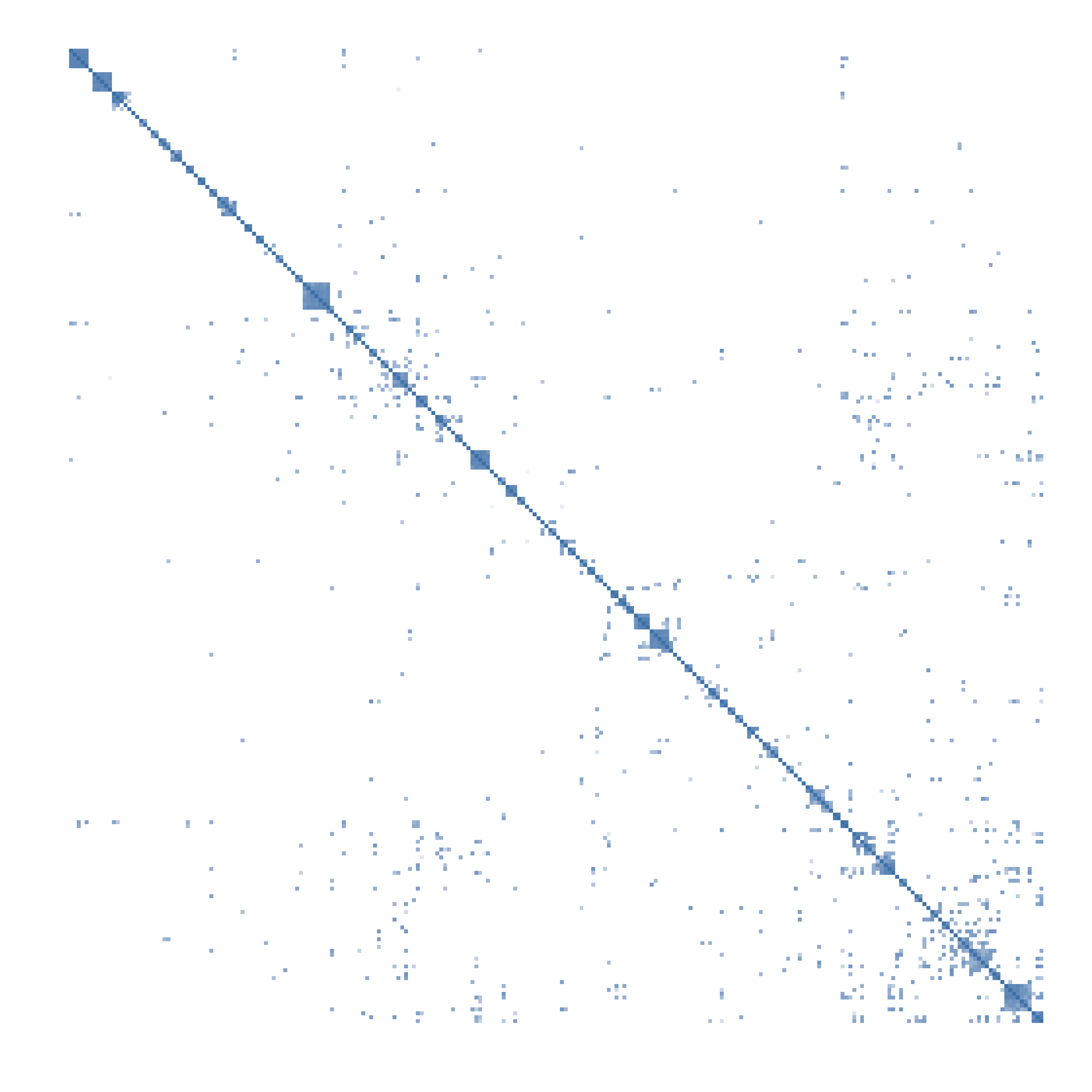
Figure 1: A sparse estimate of the inverse covariance of gene expression measurements for the first 250 genes from the DLBCL dataset. The estimate has 97.5% of the off-diagonal elements equal to 0. Darker colors represent inverse covariances of larger magnitude.

To motivate our methodology in relation to previous approaches, we examine a dataset consisting of 240 patients with diffuse large B-cell lymphoma (DLBCL, Rosenwald et al., 2002) in some detail. Each patient is measured on 7399 genes, and her survival time is recorded.

sparsity of $\boldsymbol{\Sigma}_{xx}^{-1}$		1.0000	0.9999	0.9998	0.9995	0.9991	0.9984	0.9975	0.9963	0.9946	0.9922
% non-zero $\beta$’s		0.0162	0.0216	0.0287	0.0418	0.0618	0.0843	0.1193	0.1803	0.2645	0.3699
False Negative Rate		0.0000	0.2500	0.4340	0.6117	0.7374	0.8077	0.8641	0.9100	0.9387	0.9562

Table 1: This table shows properties of the coefficients of the linear model corresponding to 10 different estimates of the inverse covariance matrix, from complete sparsity on the left (a diagonal matrix) to still more than 99% sparsity on the right. The second row is the number of non-zero population regression coefficients corresponding to each inverse covariance matrix. The bottom row shows the percentage of non-zero regression coefficients which are incorrectly ignored under the assumption on the relationship between marginal correlations and regression coefficients.

Previous approaches rely on the assumption that a small marginal correlation between the response variable, in this case patient survival time, and the vector of expression measurements for a particular gene is sufficient for guaranteeing the irrelevance of that particular gene for prediction. To make this assumption mathematically precise, suppose $y=x^{\top}\beta+\epsilon,$ where $y$ is the response, $x$ is a vector of gene expression measurements, and $\epsilon$ is a mean-zero error. Then, the assumption can be stated mathematically as $\textrm{Cov}(x_{j},y)=0\Rightarrow\beta_{j}=0$. While reasonable under some conditions, this assumption is perhaps too strong for many gene expression datasets. Very often, individual gene expressions are only predictive of phenotype in the presence of other genes. We can rewrite this assumption using the population covariance matrix between genes, $\textrm{Cov}(x,x)=\boldsymbol{\Sigma}_{xx}$, and the vector-valued covariance between gene expressions and phenotype, $\textrm{Cov}(x,y)=\Sigma_{xy}$. Then, using the population equation for $\beta$ allows us to rewrite the assumption as

$$(\Sigma_{xy})_{j}=0\Rightarrow\beta_{j}=(\boldsymbol{\Sigma}_{xx}^{-1}\Sigma_{xy})_{j}=0.$$ (1)

In words, we are assuming that the dot product of the $j^{th}$ row of the inverse covariance matrix with the covariance between $x$ and $y$ is zero whenever the $j^{th}$ element of $\Sigma_{xy}$ is zero.

To examine whether this assumption holds, we can estimate both $\boldsymbol{\Sigma}^{-1}_{xx}$ and $\Sigma_{xy}$ using the DLBCL data and imagine that these estimates are the population quantities for illustration. To estimate $\Sigma_{xy}$, we use the standard covariance estimate, but set all but the largest 120 values equal to zero, corresponding to a sparse solution. For the case of $\boldsymbol{\Sigma}^{-1}_{xx}$, estimating large inverse covariance matrices accurately is impossible when $p\gg n$ unless we assume some additional structure. If most of the entries are 0 (a necessary condition for (1) to hold), methods like the graphical lasso (glasso, Friedman et al., 2008) or graph estimation (Meinshausen and Bühlmann, 2006) have been shown to work well. We use the graph estimation technique for all 7399 genes in the dataset at ten different sparsity levels ranging from 100% to 99.2%. For visualization purposes, Figure 1 shows the first 250 genes for one estimate of the inverse covariance that is 97.5% sparse.

To assess the validity of (1), Table 1 shows the sparsity of the full inverse covariance matrix, the percentage of non-zero regression coefficients, and the percentage of non-zero regression coefficients which are incorrectly ignored by the assumption (the false negative rate). In all cases, $\Sigma_{xy}$ is about 98% sparse. Even with an extremely sparse inverse covariance matrix, the false negative rate is at least 25% meaning that 25% of possibly relevant genes are ignored by the analysis. If the sparsity of $\mathbf{\Sigma}^{-1}_{xx}$ is allowed to increase only slightly, the false negative rate increases to over 95%.

1.3 Our contribution

For a similar computational budget, our method outperforms existing approaches by taking advantage of all the data. Our method does not require that the set of non-zero regression coefficients be a subset of the non-zero marginal correlations.

Suppose that $\mathbf{M}\in\mathbb{R}^{p\times p}$ is a symmetric, nonnegative definite matrix; that is, for all vectors $a\in\mathbb{R}^{p}$, $a^{\top}\mathbf{M}a\geq 0$ and $\mathbf{M}^{\top}=\mathbf{M}$. To approximate the matrix $\mathbf{M}$, we fix an integer $\ell\ll p$ and form a sketching matrix $\mathbf{S}\in\mathbb{R}^{p\times\ell}$. Then, we report the following approximation: $\mathbf{M}\approx(\mathbf{M}\mathbf{S})(\mathbf{S}^{\top}\mathbf{M}\mathbf{S})^{\dagger}(\mathbf{M}\mathbf{S})^{\top}$. The details behind the formation of the matrix $\mathbf{S}$ control the type of approximation.

In the simplest case, which we employ here, we take $\mathbf{S}=\pi\tau,$ where $\pi\in\mathbb{R}^{p\times p}$ is a permutation of the identity matrix and $\tau=[\mathbf{I}_{\ell},\mathbf{0}]^{\top}\in\mathbb{R}^{p\times\ell}$ is a truncation matrix. While many alternative sketching matrices, mostly based on random projections, have been proposed, this method is the only one necessary to develop our results. Without loss of generality, divide the matrix $\mathbf{M}$ into blocks

$$\mathbf{M}=\begin{bmatrix}\mathbf{M}_{11}&\mathbf{M}_{21}^{\top}\\ \mathbf{M}_{21}&\mathbf{M}_{22}\\ \end{bmatrix}$$

so that we can (implicitly) construct the matrix $\mathbf{F}(\mathbf{M})\in\mathbb{R}^{p\times\ell}$ as

$$\mathbf{F}(\mathbf{M}):=\mathbf{M}\mathbf{S}=\left[\begin{array}[]{c}\mathbf{M}_{11}\\ \mathbf{M}_{21}\\ \end{array}\right].$$

Because

$$\mathbf{M} \approx(\mathbf{M}\mathbf{S})(\mathbf{S}^{\top}\mathbf{M}\mathbf{S})^{\dagger}(\mathbf{M}\mathbf{S})^{\top}=\mathbf{F}(\mathbf{M})(\mathbf{S}^{\top}\mathbf{M}\mathbf{S})^{\dagger}\mathbf{F}(\mathbf{M})^{\top},$$

we can approximate the eigendecomposition of $\mathbf{M}$ using the SVD of $\mathbf{F}(\mathbf{M})$. If we decompose $\mathbf{F}=\mathbf{U}(\mathbf{F})\boldsymbol{\Lambda}(\mathbf{F})\mathbf{V}(\mathbf{F})^{\top},$ where we have suppressed the dependence of $\mathbf{F}$ on $\mathbf{M}$ when $\mathbf{F}$ is an argument for clarity, then the resulting approximation to the eigenvectors of $\mathbf{M}$ is $\mathbf{V}(\mathbf{M})\approx\mathbf{F}\mathbf{V}(\mathbf{F})\boldsymbol{\Lambda}(\mathbf{F})^{\dagger}=\mathbf{U}(\mathbf{F}).$ Likewise, the approximate eigenvalues of $\mathbf{M}$ are given the singular values $\boldsymbol{\Lambda}(\mathbf{F})$.

Homrighausen and McDonald (2016) show that this approximation is more accurate than the one based on $\mathbf{M}_{11}$ for performing a principal components analysis. As previous techniques for principal components regression (like SPC) are based on $\mathbf{M}_{11}$ rather than $\mathbf{F}$, it is possible that by using $\mathbf{F}$, we will have better results. As we will see, this intuition turns out to be true under some conditions which were suggested in Section 1.2. In particular, for essentially the same computational budget, our procedure outperforms previous procedures if some genes have small marginal correlations with the phenotype but are, nonetheless, important for predicting the phenotype conditional on the presence of other genes. Furthermore, even if the assumption in (1) is true, our procedure is not much worse than existing approaches.

In Section 2, we discuss exactly how to implement our methodology. We examine the behavior of our procedure in Section 3. In Section 3.1, we state an explicit model for the data-generating mechanism in order to be clear about the conditions under which our procedure works well. Section 3.2 uses a number of carefully constructed simulations to show when our technique works well, and when it doesn’t. In Section 4, we examine our procedure on four genetics datasets, including the one discussed above. We find that our methods slightly outperform existing techniques on three of them, suggesting that the motivation is sound. Finally, in Section 5, we give conclusions and discuss some avenues for future work.

2 Methods and computations

We now give the details of our methodology. For clarity, we assume that the design matrix $\mathbf{X}$ and the response $Y$ are already centered. Let $T$ be a $p$-dimensional vector denoting standardized regression coefficient estimates, i.e. for any $j\in\{1,2,\ldots,p\}$, $t_{j}$ is the coefficient estimate of standardized univariate regression between response $Y$ and covariate $X_{j}$. We use standardized regression so that the coefficient estimates are comparable across disparate covariates. Note that $t_{j}$ is also the marginal correlation between the response $Y$ and covariate $X_{j}$.

For some threshold $t_{*}$, we separate $\mathbf{X}$ into two matrices $\mathbf{X}_{A}$ and $\mathbf{X}_{A^{c}}$, where $A=\{j:\left|t_{j}\right|>t_{*}\}$. We assume $|A|=\ell$. The hope is that $\mathbf{X}_{A}$ contains many of the genes that are most predictive of the phenotype under study. Ideally, high marginal correlations will suggest relevant predictors to be emphasized in the decomposition, but unlike other methods, we will also use those genes in the set $A^{c}$. We now focus on $\mathbf{X}_{new}=[\mathbf{X}_{A},\ \mathbf{X}_{A^{c}}]$ and note that it has the same range as $\mathbf{X}$. Therefore, we will use the approximation technique discussed in Section 1.3 to try to estimate the eigendecomposition of $\mathbf{\Sigma}_{xx}$ using sample quantities. Because $\mathbf{X}_{new}^{\top}\mathbf{X}_{new}$ is symmetric and positive definite, write

$$\mathbf{F}=\mathbf{X}_{new}^{\top}\mathbf{X}_{A}=\begin{pmatrix}\mathbf{X}^{\top}_{A}\mathbf{X}_{A}\\ \mathbf{X}^{\top}_{A^{c}}\mathbf{X}_{A}\end{pmatrix},$$

and decompose $\mathbf{F}=\mathbf{U}(\mathbf{F})\boldsymbol{\Lambda}(\mathbf{F})\mathbf{V}(\mathbf{F})$. For some integer $d\in\{1,\ldots,\ell\}$, we define

$$\mathbf{\widehat{V}}_{[d]} =\mathbf{U}_{[d]}(\mathbf{F}),$$

$$\mathbf{\widehat{\Lambda}}_{[d]} =\boldsymbol{\Lambda}_{[d]}(\mathbf{F})^{1/2},\quad\quad\textrm{and}$$

$$\mathbf{\widehat{U}}_{[d]} =\mathbf{X}_{new}\mathbf{\widehat{V}}_{[d]}\boldsymbol{\widehat{\Lambda}}^{-1}_{[d]}.$$

Now we have estimates for the principal components $\mathbf{\widehat{U}}_{[d]}\boldsymbol{\widehat{\Lambda}}_{[d]}$. Therefore, just as with principal components regression, we can regress $Y$ on the estimated principal components to produce estimated coefficients in principal component space:

$$\boldsymbol{\widehat{\Gamma}}_{AIMER}=\operatorname*{argmin}_{\Gamma}\left\lVert Y-\mathbf{\widehat{U}}_{[d]}\boldsymbol{\widehat{\Lambda}}_{[d]}\boldsymbol{\Gamma}\right\rVert_{2}^{2} =\boldsymbol{\widehat{\Lambda}}^{-1}_{[d]}\mathbf{\widehat{U}}^{T}_{[d]}Y.$$

Then the coefficient estimates for linear regression in the space spanned by $\mathbf{X}_{new}$ are given by

$$\boldsymbol{\widehat{\beta}}_{AIMER}=\mathbf{\widehat{V}}_{[d]}\boldsymbol{\widehat{\Gamma}}_{AIMER}=\mathbf{\widehat{V}}_{[d]}\boldsymbol{\widehat{\Lambda}}^{-1}_{[d]}\mathbf{\widehat{U}}^{T}_{[d]}Y.$$ (2)

Because our methodology uses marginal regression to select a small number of hopefully relevant predictors before “amplifying” their eigenstructure information with the $\mathbf{F}$ matrix, we refer to our technique as “Amplified, Initially Marginal, Eigenvector Regression” (AIMER).

Unlike previous approaches, the solution given by (2) is not sparse: with probability 1, $(\boldsymbol{\widehat{\beta}}_{AIMER})_{j}\neq 0,\ \forall j$. However, most of the coefficients will be small. We therefore threshold the estimates to produce our final estimator:

$$\boldsymbol{\widehat{\beta}}_{AIMER}(b):=\boldsymbol{\widehat{\beta}}_{AIMER}\boldsymbol{1}_{(b,\infty)}(|\boldsymbol{\widehat{\beta}}_{AIMER}|),$$ (3)

where $b\geq 0$, and $\boldsymbol{1}_{A}(w)$ is the indicator function, which returns the value one for every element of $w\in A$ and zero otherwise. We summarize this procedure in Algorithm 1. As with SPC, the computational burden of our method is dominated by the SVD. We use an SVD of $\mathbf{F}$ while SPC uses the SVD of $\mathbf{X}_{A}$. However, since the SVD is cubic in the smaller dimension, in both cases the computation is $O(|A|^{3})$. Thus, to leading order, both methods require the same amount of computation.

Input: centered design matrix $\mathbf{X}$, centered response $Y$, thresholds $t_{*},b_{*}\geq 0$, integer $d$

1 Compute marginal correlation $t_{j}$ between $X_{j}$ and $Y$ for all $j$;

2

3Set $A=\{j:\left|t_{j}\right|>t_{*}\}$;

4

5Set $\mathbf{X}_{new}=[\mathbf{X}_{A},\ \mathbf{X}_{A^{c}}]$;

6

7Define $\mathbf{F}=\mathbf{X}_{new}^{\top}\mathbf{X}_{A}$;

8

9Decompose $\mathbf{F}=\mathbf{U(\mathbf{F})\Lambda(\mathbf{F})V(\mathbf{F})}^{\top}$;

10

11Set $\mathbf{\widehat{V}}_{[d]}=\mathbf{U}_{[d]}(\mathbf{F})$;

12

13Set $\boldsymbol{\widehat{\Lambda}}_{[d]}=\boldsymbol{\Lambda}_{[d]}(\mathbf{F})^{1/2}$;

14

15Set $\mathbf{\widehat{U}}_{[d]}=\mathbf{X}_{new}\mathbf{\widehat{V}}_{[d]}\boldsymbol{\widehat{\Lambda}}^{-1}_{[d]}$;

16

17Calculate $\boldsymbol{\widehat{\beta}}=\mathbf{\widehat{V}}_{[d]}\boldsymbol{\widehat{\Lambda}}^{-1}_{[d]}\mathbf{\widehat{U}}^{T}_{[d]}\mathbf{Y}$ ;

18

19Set $\boldsymbol{\widehat{\beta}}(b_{*}):=\boldsymbol{\widehat{\beta}}\boldsymbol{1}_{(b_{*},\infty)}(|\boldsymbol{\widehat{\beta}}|)$;

20

Output: coefficient estimates $\boldsymbol{\widehat{\beta}}(b_{*})$

Algorithm 1 Amplified, Initially Marginal, Eigenvector Regression (AIMER)

To make predictions given a new observation $x_{*}$, we simply center it using the mean of the original data, reorder its entries to conform to $\mathbf{X}_{new}$, multiply by the coefficient vector in (3), and add the mean of the original response vector.

3 Experimental analysis

To examine the performance of our method, we set up a number of carefully constructed simulations under various conditions. We first discuss the generic data model we assume, a latent factor model, which is amenable to analysis via SPC or AIMER.

3.1 Data model

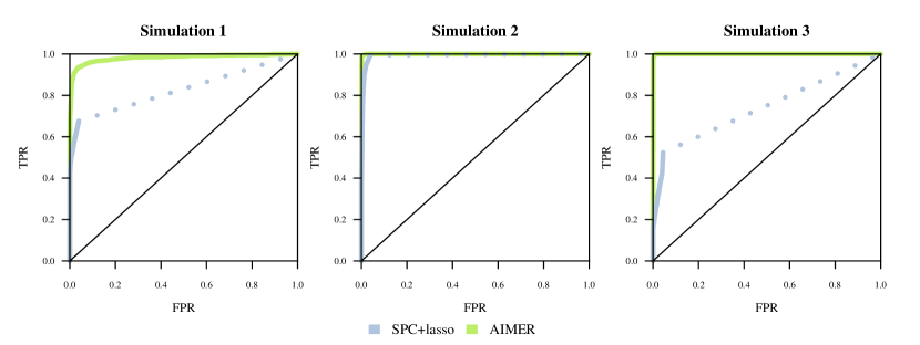
Figure 2: Receiver operating characteristic (ROC) Curve for Simulations 1–3. The $x$-axis is the false positive rate while the $y$-axis is the true positive rate. The curves present averages across 100 replications. SPC is limited to only 50 selected genes, and so its false positive rate is bounded. The dashed line indicates its best case theoretical performance were it allowed to continue to select further genes.

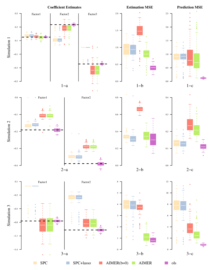
Figure 3: Estimation and prediction performance of SPC and AIMER in the first three simulations. The left panel shows the estimates of the regression coefficients, the middle panel shows the mean squared error (MSE) of estimation for all 1000 genes, and the right panel shows prediction MSE on the held-out data. The boxes indicate variability across 100 replications. The dashed black horizontal lines indicate the true values of $\beta$.

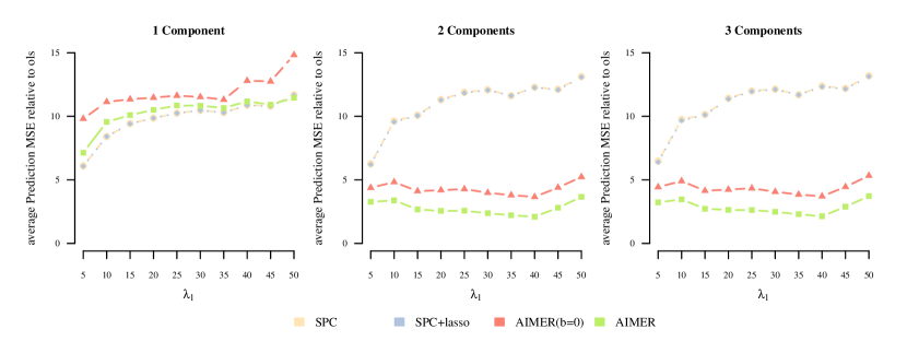
Figure 4: Prediction MSE averaged across 100 replications for each method for different numbers of components (Simulation 4). We also allow $\lambda_{1}$ to vary between 5 and 50.

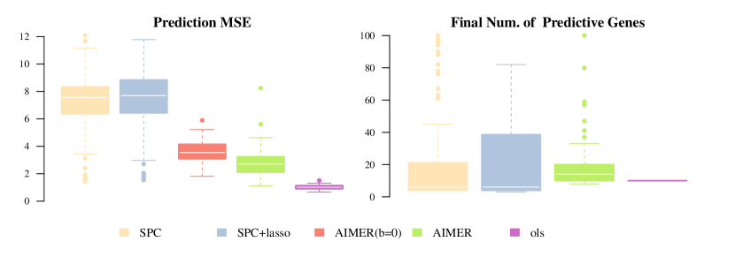
Figure 5: Performance of each method when we allow $t_{*}$ to be chosen by cross validation rather than fixed to choose 50 genes (Simulation 5).

Simulation		1	2	3
True #		15	10	10
SPC		50 (0)	50 (0)	50 (0)
SPC+lasso		31 (9.011)	39 (3.636)	46 (2.665)
AIMER($b=0$)		1000 (0)	1000 (0)	1000 (0)
AIMER		39 (9.225)	21 (12.750)	16 (7.558)

Table 2: Average final number of predictive genes in Simulations 1, 2, and 3. The standard deviation is shown in parentheses.

Consider the multivariate Gaussian linear regression model

$$y=x^{\top}\boldsymbol{\beta}+\sigma_{1}\epsilon$$ (4)

with $y$ the response, ${x}\in\mathbb{R}^{p}$ a column vector of gene expression measurements, $\boldsymbol{\beta}=(\beta_{1},\cdots,\beta_{p})^{\top}$ the coefficients, $\epsilon$ a random Gaussian distributed error with zero mean and variance 1, and $\sigma_{1}>0$. We further assume that $x\sim N_{p}(\mathbf{0},\boldsymbol{\Sigma}_{xx})$ has a Gaussian distribution with mean vector $\mathbf{0}$ and covariance matrix $\boldsymbol{\Sigma}_{xx}$. We will assume that $\boldsymbol{\beta}$ is sparse, in that most of its elements are exactly 0 indicating no linear relationship between the associated gene and the response. Finally, the design matrix $\mathbf{X}$ and the response vector $Y$ include $n$ independent observations of $x$ and $y$ respectively.

Model for $\mathbf{X}$.

As $\boldsymbol{\Sigma}_{xx}$ is symmetric and positive (semi-) definite, we can decompose it as

$$\boldsymbol{\Sigma}_{xx} =\mathbf{V}(\boldsymbol{\Sigma}_{xx})\mathbf{L}(\boldsymbol{\Sigma}_{xx})\mathbf{V}^{T}(\boldsymbol{\Sigma}_{xx})$$

$$=\begin{pmatrix}V_{1}&\cdots&V_{p}\end{pmatrix}\begin{pmatrix}l_{1}&&0\\ &\ddots&\\ 0&&l_{p}\end{pmatrix}\begin{pmatrix}V^{\top}_{1}\\ \vdots\\ V^{\top}_{p}\end{pmatrix},$$

where $V_{1},\cdots,V_{p}$ are orthonormal eigenvectors on $\mathbb{R}^{p}$ and $l_{1}\geq\cdots\geq l_{p}\geq 0$ are eigenvalues. We assume that there is some $1\leq G\leq p$ such that the eigenvalues can be seperated into two groups, one of which includes relatively large eigenvalues and the other relatively small eigenvalues, that is, $l_{k}=\lambda_{k}+\sigma^{2}_{0}$ for $1\leq k\leq G$ and $l_{k}=\sigma^{2}_{0}$ for $k>G$ where $\lambda_{1}\geq\cdots\geq\lambda_{G}>0$, and $\sigma^{2}_{0}>0.$

Then, because $\mathbf{X}$ is multivariate Gaussian, we can write $\mathbf{X}$ as

$$\mathbf{X} =\mathbf{U}_{G}\mathbf{\Lambda}_{G}\mathbf{V}^{T}_{G}+\sigma_{0}\mathbf{E}$$

$$=\begin{pmatrix}U_{1}&\cdots&U_{G}\end{pmatrix}\begin{pmatrix}\sqrt{\lambda_{1}}&&0\\ &\ddots&\\ 0&&\sqrt{\lambda_{G}}\end{pmatrix}\begin{pmatrix}V^{\top}_{1}\\ \vdots\\ V^{\top}_{G}\end{pmatrix}+\sigma_{0}\mathbf{E}$$

where latent factors $U_{1},\ldots,U_{G}$ are independent and identically distributed (i.i.d.) $N_{n}(\mathbf{0},\mathbf{I})$ vectors, and the noise matrix $\mathbf{E}$ is $n\times p$ with i.i.d. $N(0,1)$ entries independent of $U_{1},\ldots,U_{G}$.

Model for $Y$.

We assume that $Y$ is a linear function of the first $K\leq G$ latent factors in $\mathbf{U}_{G}$ plus additive Gaussian noise: $Y=\mathbf{U}_{K}\boldsymbol{\Theta}+\sigma_{1}Z,$ where $\boldsymbol{\Theta}$ is the coefficient vector, $\sigma_{1}>0$ is a constant, and $Z$ is distributed $N_{n}(\mathbf{0},\mathbf{I})$, independent of $\mathbf{X}$. Note that the expectation of $Y$ is zero and that this is a specific form of (4).

Implication of the model.

Under this model for $\mathbf{X}$ and $Y$, the population marginal covariance between each gene $X_{j}$ and the response $Y$ can be written as

$$\Sigma_{xy} =\begin{pmatrix}\textrm{Cov}(X_{1},Y)\\ \vdots\\ \textrm{Cov}(X_{p},Y)\end{pmatrix}=\mathbf{V}_{K}\mathbf{\Lambda}_{K}\mathbf{\Theta}.$$ (5)

Therefore, the population ordinary least squares coefficients of regressing $Y$ on $\mathbf{X}$ ($\boldsymbol{\beta}$ in (4)) can be written as

$$\boldsymbol{\beta} =\boldsymbol{\Sigma}_{xx}^{-1}\Sigma_{xy}=\mathbf{V}_{K}\mathbf{L}^{-1}_{K}\mathbf{\Lambda}_{K}\boldsymbol{\Theta}$$ (6)

We will define the set $\mathscr{B}:=\{j:(\Sigma_{xy})_{j}\neq 0\}$ and the set $\mathscr{A}:=\{j:\beta_{j}\neq 0\}$. We note that for $K=1$, it is always the case that $\mathscr{A}=\mathscr{B}$. By manipulating the parameters in $\boldsymbol{\Theta}$, $\mathbf{L}$, and $\mathbf{\Lambda}$, we can create a number of scenarios for testing AIMER against alternative methods.

3.2 Experiments

We present results under five different experiments. For each of the simulations which follow, we generate datasets with $n=200$ and $p=1000$. We use half ($n=100$) to estimate the model and test our predictions on the other half. We repeat this process 100 times for each combination of parameters. Throughout, we use $\sigma_{0}=\sqrt{.1}\approx.3$ and $\sigma_{1}=.1$. The matrix $\mathbf{U}$ is generated with i.i.d. standard Gaussian entries, while the matrix $\mathbf{V}$ is constructed by hand to have the correct number of orthogonal components.

The first experiment is designed to be favorable to AIMER. The second is designed to be favorable to SPC. The third examines the extent to which the assumption that $\mathcal{A}=\mathcal{B}$ is beneficial to SPC over AIMER. The fourth examines the impact of using incorrect numbers of components, while the fifth uses cross validation on all the tuning parameters.

Simulation 1: Favorable conditions for AIMER.

In this simulation, we create data which is amenable to AIMER at the expense of the conditions for SPC, that is we use $\mathscr{B}\subset\mathscr{A}$. We set parameters in the data model as $K=G=3$ and choose $\lambda_{1}=10,$ $\lambda_{2}=5,$ and $\lambda_{3}=1$. In order to achieve $\mathscr{B}\subset\mathscr{A}$, we set $\theta_{1}=\theta_{2}=1$ and solve (5) for $\theta_{3}$ so that some corresponding elements of $\Sigma_{xy}$ will be zero. We make the first 15 elements of $\boldsymbol{\beta}$ non-zero, 5 corresponding to each of the three principal components. Thus, the first 10 genes have non-zero population marginal correlation and the remaining 990 have zero marginal correlation. In this scenario, SPC should find the first 10 important genes, but AIMER will find the remaining 5 important genes as well.

In order to focus on the relationship between performance and the condition $\mathscr{B}\subset\mathscr{A}$, we examine the methods for a fixed computational budget and choose $t_{*}$ to select the same $50$ most predictive genes. We examine SPC, SPC with lasso, AIMER($b=0$), and AIMER. We use the first 3 principal components for regression in all the methods. For SPC with lasso and AIMER, we choose the remaining tuning parameters via 10-fold cross-validation. We also give results for OLS on the first 15 genes. This is the oracle estimator, the best one could hope to do with foreknowledge of the predictive genes.

Figure 2 shows the classification performance using a receiver operating characteristic (ROC) curve for SPC with lasso and AIMER in the left panel (the remaining panels are for the next two simulations). Examining the figure, it is easy to see that SPC+lasso identifies the first 10 genes easily, but AIMER is able to capture all 15 predictive genes at a low cost of false positive identifications. A more detailed analysis is given in the first row of Figure 3. Panel 1–a shows the ability of each method to estimate the $\boldsymbol{\beta}$ coefficients of three different factors. Coefficient estimates for the 5 genes in factor 1 by AIMER are slightly more accurate, and no more variable, than SPC+lasso. Furthermore, AIMER is better at estimating those $\boldsymbol{\beta}$’s associated with factor 2, and much better at those associated with factor 3 (these are assumed zero in SPC). Panel 1–b examines the mean square error (MSE) of estimation as the average squared difference between the true coefficients and their estimates for all 1000 genes. The overall estimation accuracy of AIMER($b=0$) is worse because of the inclusion of so many useless genes (it estimates all 1000), however, by thresholding with AIMER, accuracy is improved and exceeds that of SPC with and without lasso. In panel 1–c, we show the MSE for prediction, the average squared difference between predicted values and the actual observations, for a test set. This MSE is smaller for AIMER than for SPC much of the time, but the variance across simulations is large.

Simulation 2: Favorable conditions for SPC.

This simulation compares the performance of SPC and AIMER under conditions which are more favorable to SPC. In particular, we choose parameters such that $\mathscr{A}=\mathscr{B}$. While AIMER is likely to perform worse because it will tend to include irrelevant genes, it is not too much worse. Most of the parameters are the same as in Simulation 1, except that $K=G=2$, $\lambda_{1}=10$, $\lambda_{2}=1$, $\theta_{1}=\theta_{2}=1$, and we use the first two principal components to do regression. Therefore, 10 out of 1000 genes are truly predictive of the response, and all 10 have non-zero marginal correlation with the response (the rest have $\Sigma_{xy}=0$). Looking again at Figure 2, both SPC+lasso and AIMER can identify all 10 predictive genes at a small price of false positives. Examining Figure 3, we see that the estimation accuracy of SPC/SPC+lasso is better than that of AIMER as expected, and the MSE of prediction for AIMER is about twice that of SPC/SPC+lasso. The estimation MSE (panel 2–b) of AIMER is comparable to that of SPC.

Simulation 3: Slight perturbations.

In this simulation, we adjust only $\theta_{2}=3$, rather than 1 as in simulation 2, thereby maintaining the condition that $\mathscr{A}=\mathscr{B}$. However, in this case AIMER works much better than SPC/SPC+lasso. Figures 2 and 3 show that AIMER can easily identify all the predictive genes, has more precise coefficient estimates, and has much smaller MSE for prediction. The reason is that, even though $\mathscr{A}=\mathscr{B}$, the marginal correlations for some predictive genes are very small. Therefore those genes are more difficult for SPC to identify, but AIMER can compensate.

For one further comparison, Table 8 shows the average (standard deviation in parentheses) number of predictive genes selected in each of the first three simulations. AIMER selects the smallest number of coefficients in most cases.

Simulation 4: Choosing the number of components.

	DLBCL			Breast cancer			Lung cancer			AML
Methods	MSE	# genes	$d$	MSE	# genes	$d$	MSE	# genes	$d$	MSE	# genes	$d$
lasso	0.6805	20		0.6285	9		0.8159	22		1.9564	6
ridge	0.6485	7399		0.6407	4751		0.7713	7129		1.9234	6283
SPC	0.6828	41	3	0.6066	16	2	0.8344	19	3	2.4214	24	2
SPC+lasso	0.6780	31	3	0.6029	14	2	0.8436	9	4	2.3980	22	2
AIMER($b=0$)	1.1896	7399	2	2.6531	4751	1	0.9444	7129	1	12.4014	6283	1
AIMER	0.6518	28	4	0.6004	31	3	1.0203	13	1	1.8746	36	4

Table 3: The MSE on the test set, the number of selected genes, and the number of principal components used ($d$ if relevant), each averaged across the 10 random training-testing splits. Bolded values indicate the best predictive performance for each type of method (with and without structure learning) for each data set.

In the previous simulations, we used the correct number of principal components, though such a choice is unlikely to be possible given real data. In this simulation, we examine the impact choosing the number of components has on estimation accuracy. We use similar parameter settings as Simulation 1 except with $K=G=2$ rather than 3 (we maintain the condition that $\mathcal{B}\subset\mathcal{A}$). We then use all the methods with 1, 2, and 3 components. We also adjust the values of $\lambda_{1}$ in a range from 5 to 50. As we can see in Figure 4, using two components reduces MSE for AIMER($b=0$) and AIMER across all values of $\lambda_{1}$ relative to using only one component, while using more than two components has little impact. With only one component, SPC performs better than AIMER, likely due to smaller variance for a similar bias, but using two or three components leads to large gains for AIMER. In practice, it is worthwhile to try several numbers of components and use cross-validation to decide which works best.

Simulation 5: The screening threshold.

In previous simulations, we choose $t_{*}$ so that variable screening by the marginal correlation would always select exactly 50 genes. Thus, we could compare methods based on their ability to use the same amount of information. In reality, it may be better to choose the threshold $t_{*}$ using cross validation. In this simulation, we use the same conditions as in the previous simulation with $\lambda_{1}=10$. It is still not appropriate to have more genes than patients, so we allow the number of selected genes to be anything less than the number of patients (100). We further use 10-fold cross-validation to choose the best threshold.

As shown in Figure 5, allowing $t_{*}$ to be chosen rather than fixed leads to improved results for AIMER relative to SPC/SPC+lasso. The prediction MSE decreases and fewer genes are selected.

4 Performance on real data

We now illustrate our methods on 4 empirical datasets in genomics that record the censored survival time and gene expression measurements from DNA microarrays of patients with 4 different types of cancer. The first dataset comes from Rosenwald et al. (2002) and contains 240 patients with diffuse large B-cell lymphoma (DLBCL) and 7399 genes. The second dataset has 4751 gene expression measurements of 78 breast cancer patients (Van’t Veer et al., 2002). The third consists of 86 lung cancer patients measured on 7129 genes (Beer et al., 2002), and finally, we analyze a dataset consisting of 116 patients with acute myeloid leukemia (AML, Bullinger et al., 2004) and 6283 genes.

Since the survival times for some patients are censored and right-skewed, we use $\log(\textrm{survival time}+1)$ as the response. A Cox model would be more appropriate, but this transformation is enough to illustrate our methodology. In order to assess our method using limited data, we randomly select half of the data as the training set and let the rest be in the testing set, then estimate each model using the training half and predict the held out data. We repeat this procedure for 10 random splits and report the average error. We use 10-fold cross-validation on the training set to choose all tuning parameters ($t_{*}$, $b_{*}$, $d$, and $\lambda$ where appropriate), mimicking the procedure of a real data analysis.

We apply 7 methods on each dataset: 1) PCR; 2) lasso; 3) ridge regression; 4) SPC; 5) SPC+lasso; 6) AIMER($b=0$); and 7) AIMER. We use the R packages pls (Mevik and Wehrens, 2007) to perform PCR and glmnet (Friedman et al., 2010) to perform lasso and ridge. For PCR, SPC, SPC+lasso, AIMER($b=0$), and AIMER, we allow the number of components $d$ to be chosen between 1 and 5.

Our results are shown in Table 4. For each dataset, we show the MSE on the testing set, the number of selected genes, and the number of principal components used (if relevant), averaged across the 10 random training-testing splits. We do not show results for PCR because it is uniformly awful. The results in Table 4 are largely consistent with the conclusions we derive from simulations. AIMER and SPC+lasso tend to select a similar number of genes, though AIMER has better prediction error on 3 of the 4 datasets. Interestingly, the genes selected by SPC+lasso, lasso, and AIMER rarely overlap, suggesting that to identify genes for further study, one should try all three methods. The online Supplement lists the genes identified by AIMER for each dataset. In the case of DLBCL, we also list any previous research relating the selected genes to lymphoma.

The Lung Cancer data is rather odd in that AIMER$(b=0)$ has better performance than AIMER. This anomaly is likely because, in contrast with the other datasets, the lung cancer expression measurements have not been scaled relative to a control group. We tried two transformations using only the treatment group to approximate such a scaling, but, while the performance of our method becomes comparable to SPC following transformations, it remains slightly worse. Without a control group, it is difficult to explain this outcome with any certainty. A comparison of these alternative transformations with our results in Table 4 is contained in the online Supplement.

As seen in the table, ridge regression is sometimes the best of all the methods. Previous experience suggests that ridge regression is dominant if the genes are highly correlated or when there is not a particularly predictive set of genes. However, the fact that ridge does not screen out unimportant genes is a barrier to its applications in genomics. On the other hand, AIMER approaches or exceeds the small prediction error of ridge regression while also selecting a small number of predictive genes, making it a better candidate for solving these types of problems.

5 Discussion

High-dimensional regression methods help in predicting future survival time and identifying possibly predictive genes for diseases. However, the large number of genes, the limited access to patients, and the complex covariance structure between genes make the problem both computationally and statistically difficult. In both simulations and analysis of actual gene expression datasets, AIMER has comparable or slightly improved prediction accuracy relative to existing methods and finds small numbers of actually predictive genes, all while having a similar computational burden. On the other hand, there are some issues which warrant further exploration.

A major benefit of SPC is that it comes with theoretical guarantees under certain assumptions. While our methodology is intended to work when these assumptions don’t hold, we do not yet have comparable guarantees. However, the simulated experiments in this paper have suggested how we might derive such results in a more general setting.

For the real data examples in this paper, we applied a simple monotonic transformation to the response variable, however, extending our methods to Cox models, which are more appropriate, and other generalized linear models for predicting discrete traits is highly desirable. It may also be useful to examine other eigenstructure techniques such as Locally Linear Embeddings or Laplacian Eigenmaps to produce non-linear predictors. Finally, using other matrix approximation techniques may yield improved performance or be more amenable to theoretical analysis.

Funding

This work is supported by the National Science Foundation [grant number DMS–14-07439 to D.J.M.].

Conflict of interest: none to declare.

Appendix A Genes identified for the DLBCL data

In this supplement, we perform AIMER on all four datasets (DLBCL (Rosenwald et al., 2002), breast cancer (Bullinger et al., 2004), lung cancer (Beer et al., 2002), AML (Van’t Veer et al., 2002)) discussed in the manuscript. Rather than using training sets containing 50% of the data as in the main paper, we use all the observations here. We allow our method to select up to as many features as there are observations.

A.1 DLBCL

For the DLBCL data, we not only list the selected genes, but also attempt to find any discussion of those genes in existing literature. Our final estimated model uses 49 gene features, which correspond to 26 genes. To examine the relevance of each selected gene for DLBCL, we adopt two approaches. The first endeavors to find literature examining the biological connection of the identified gene to any type of lymphoma. The second lists any reference in the (rather lengthy) methodological literature in statistics, computer science, and bioinformatics that uses statistical or machine learning methods to examine the DLBCL dataset.

We display our findings for all 26 genes in Table 4. To summarize, 16 out of the 26 genes have been related to lymphoma in the biological literature, and 19 of them have already been identified via statistical techniques developed for the DLBCL dataset. While many of the 26 genes have been previously connected to lymphoma in general and DLBCL in particular, AIMER does identify 4 genes with symbols ALDH2, CELF2, COL16A1, and DHRS9 that have not been previously identified in the biological or methodological literature. We note that, while we have made every effort to locate each gene, given the large and evolving literature on this topic, those we have been unable to locate may have none-the-less been previously studied.

	Symbol	In biology	Source(s)	In methodology	Source(s)	Name of gene
1	ALDH2	$\times$		$\times$		aldehyde dehydrogenase 2 family (mitochondrial)
2	BCL2	✓	Kramer et al. (1996); Blenk et al. (2007)	✓	Lossos et al. (2004); Blenk et al. (2007)	BCL2, apoptosis regulator
3	CCND2	✓	Blenk et al. (2007)	✓	Miyazaki et al. (2008); Lossos et al. (2004); Blenk et al. (2007)	cyclin D2
4	CELF2	$\times$		$\times$		CUGBP Elav-like family member 2
5	COL3A1	✓	Rosenwald et al. (2002); Blenk et al. (2007)	✓	Blenk et al. (2007)	collagen type III alpha 1 chain
6	COL16A1	$\times$		$\times$		collagen type XVI alpha 1 chain
7	CR2	$\times$		✓	Ma and Huang (2007); Miyazaki et al. (2008)	complement C3d receptor 2
8	CYP27A1	$\times$		✓	Zhao and Wang (2010)	cytochrome P450 family 27 subfamily A member 1
9	DHRS9	$\times$		$\times$		dehydrogenase/reductase 9
10	EPHB1	✓	Asmar et al. (2013)	✓	Zhao and Wang (2010)	EPH receptor B1
11	ESTs	✓	Rosenwald et al. (2002)	✓	Liu et al. (2010)	ESTs
12	FN1	✓	Rosenwald et al. (2002); Blenk et al. (2007)	✓	Lossos et al. (2004); Blenk et al. (2007)	fibronectin 1
13	FUT8	$\times$		✓	Li et al. (2015)	fucosyltransferase 8
14	IGHM	$\times$		✓	Blenk et al. (2007); Miyazaki et al. (2008); Zhao and Wang (2010)	immunoglobulin heavy constant mu
15	IGKC	$\times$		✓	Miyazaki et al. (2008); Zhao and Wang (2010)	immunoglobulin kappa constant
16	IRF4	✓	Alizadeh et al. (2000); Radivojac et al. (2008)	✓	Blenk et al. (2007); Li et al. (2015)	interferon regulatory factor 4
17	KIAA0233	✓	Rosenwald et al. (2002); Blenk et al. (2007)	✓	Blenk et al. (2007)	KIAA0233 gene product
18	LMO2	✓	Natkunam et al. (2007); Alizadeh et al. (2000)	✓	Blenk et al. (2007); Liu et al. (2010); Lossos et al. (2004)	LIM domain only 2
19	MAPK10	✓	Ying and Gao (2010)	✓	Blenk et al. (2007); Liu et al. (2010); Zhao and Wang (2010)	mitogen-activated protein kinase 10
20	MME	$\times$		✓	Blenk et al. (2007)	membrane metalloendopeptidase
21	MMP2	✓	Gouda et al. (2014)	✓	Ma and Huang (2007)	matrix metallopeptidase 2
22	MMP7	✓	Matsumoto et al. (2008)	$\times$		matrix metallopeptidase 7
23	MMP9	✓	Sakata et al. (2004); Alizadeh et al. (2000)	✓	Liu et al. (2010)	matrix metallopeptidase 9
24	MYB	✓	Dai et al. (2016)	✓	Blenk et al. (2007)	MYB proto-oncogene, transcription factor
25	SPARC	✓	Meyer et al. (2011); Brandt et al. (2013)	$\times$		secreted protein acidic and cysteine rich
26	VPREB3	✓	Rodig et al. (2010)	$\times$		V-set pre-B cell surrogate light chain 3

Table 4: DLBCL Predictive Genes. AIMER selected 26 genes. We note that while we have made every effort to locate all 26 genes in the literature, a $\times$ should be taken to indicate that we were unable to locate a reference for that gene rather than the stronger conclusion that no one has yet investigated it.

A.2 Genes identified for breast cancer, lung cancer and AML data

As before, we allow the maximum number of selected genes be the same as the total number of patients. AIMER identifies 78 genes with breast cancer data, 12 genes for lung cancer, and 50 genes for the AML dataset. We list the top 20 selected genes for breast cancer in Table 5, all 12 selected genes for lung cancer in Table 6, and the top 20 selected genes for AML in Table 7.

	Gene
1	Contig47405$\_$RC
2	NM$\_$002964
3	NM$\_$002965
4	NM$\_$005980
5	Contig43983$\_$RC
6	NM$\_$017422
7	NM$\_$002963
8	NM$\_$020974
9	Contig50360$\_$RC
10	Contig55725$\_$RC
11	NM$\_$018265
12	NM$\_$006115
13	AK001423
14	NM$\_$004525
15	Contig38438$\_$RC
16	AL050227
17	NM$\_$014479
18	NM$\_$002421
19	NM$\_$000266
20	NM$\_$006419

Table 5: Top 20 selected genes for breast cancer dataset by AIMER.

	Gene
1	D49824$\_$s$\_$at
2	X57809$\_$s$\_$at
3	M17886$\_$at
4	S71043$\_$rna1$\_$s$\_$at
5	M87789$\_$s$\_$at
6	V00594$\_$s$\_$at
7	X98482$\_$r$\_$at
8	M34516$\_$at
9	hum$\_$alu$\_$at
10	HG2873-HT3017$\_$at
11	HG3364-HT3541$\_$at
12	HG3549-HT3751$\_$at

Table 6: 12 selected genes for lung cancer dataset by AIMER.

	Gene
1	112298 MSLN mesothelin
2	111553 GAGED2 G antigen, family D, 2
3	117339 APOC2 apolipoprotein C-II
4	330384 SERPINF1 serine (or cysteine) proteinase inhibitor, clade F (alpha-2 antiplasmin, pigment epithelium derived factor), member 1
5	330504 TRG@ T cell receptor gamma locus
6	220502 TCF4 transcription factor 4
7	101316 HLA-DRB3 major histocompatibility complex, class II, DR beta 3
8	109247 TRG@ T cell receptor gamma locus
9	98472 KIAA0476 KIAA0476 gene product
10	331153 HLA-DRB3 major histocompatibility complex, class II, DR beta 3
11	313178 KIAA1165 likely ortholog of mouse Nedd4 WW domain-binding protein 5A
12	330849 HLA-DRB3 major histocompatibility complex, class II, DR beta 3
13	107072 NCF4 **neutrophil cytosolic factor 4, 40kDa
14	114151 HLA-DRB3 major histocompatibility complex, class II, DR beta 3
15	246144 ESTs Highly similar to CAMP-DEPENDENT PROTEIN KINASE INHIB
16	103236 TRG@ T cell receptor gamma locus
17	118267 SDPR serum deprivation response (phosphatidylserine binding protein)
18	114582 HLA-DPB1 major histocompatibility complex, class II, DP beta 1
19	309986 THY1 Thy-1 cell surface antigen
20	119834 LPHH1 latrophilin 1

Table 7: Top 20 selected genes for AML dataset by AIMER.

Appendix B Alternative analysis for lung cancer data

Compared with the other three datasets, the public lung cancer data comes presents gene expression measurements for only patients who have been diagnosed with lung cancer. The other three datasets instead give the logarithm of the ratio between diseased sample expression measurements and a reference control group. To try to make the lung cancer dataset comparable to the others, we perform two separate transformations on the data. The first transformation is to take the base-2 logarithm of all the expression measurements. Because some measurements are negative, before taking the logarithm, we first add the negative of the minimum value plus one to each feature vector, making all measurements at least 1. This transformation mimics the standard process. The second transformation orthonormalizes the gene expression matrix.

We use the same training and testing procedure as in the main paper on the original dataset and the two transformed datasets. Table 8 shows the corresponding prediction MSE, the number of selected genes, and the number of components used (when necessary) averaged over 10 training-testing splits. It turns out that both the $\log_{2}$ transformation and normalization improves AIMER relative to the other methods. The number of components used in AIMER also increases. The number of selected genes for AIMER on the $\log_{2}$ transformed dataset is the same as with the original dataset, but AIMER selects more genes on the normalized dataset. However, even after these two transformations, AIMER is still not quite as accurate as SPC. We posit that using the conventional transformation with a control group may enhance the results for AIMER.

	original dataset				$\log_{2}$ transformation				normalization
Methods	MSE	# genes	$d$		MSE	# genes	$d$		MSE	# genes	$d$
lasso	0.8159	22			0.8722	16			0.7921	20
ridge	0.7713	7129			0.7594	7129			0.7687	7129
SPC	0.8344	19	3		0.8268	32	5		0.7799	22	3
SPC+lasso	0.8436	9	4		0.8376	25	4		0.7864	19	3
AIMER($b=0$)	0.9444	7129	1		0.9570	7129	1		4.5202	7129	3
AIMER	1.0203	13	1		0.8901	13	2		0.8244	42	4

Table 8: The MSE on the test set, the number of selected genes, and the number of principal components used ($d$ if relevant), each averaged across the 10 random training-testing splits on the three datasets respectively.

References

- Alizadeh et al. (2000) Alizadeh, A. A., Eisen, M. B., Davis, R. E., Ma, C., Lossos, I. S., Rosenwald, A., Boldrick, J. C., Sabet, H., Tran, T., Yu, X., et al. (2000), “Distinct types of diffuse large B-cell lymphoma identified by gene expression profiling,” Nature, 403(6769), 503–511.
- Alter et al. (2000) Alter, O., Brown, P. O., and Botstein, D. (2000), “Singular value decomposition for genome-wide expression data processing and modeling,” Proceedings of the National Academy of Sciences, 97(18), 10101–10106.
- Asmar et al. (2013) Asmar, F., Punj, V., Christensen, J., Pedersen, M. T., Pedersen, A., Nielsen, A. B., Hother, C., Ralfkiaer, U., Brown, P., Ralfkiaer, E., et al. (2013), “Genome-wide profiling identifies a DNA methylation signature that associates with TET2 mutations in diffuse large B-cell lymphoma,” Haematologica, 98(12), 1912.
- Bair and Tibshirani (2004) Bair, E., and Tibshirani, R. (2004), “Semi-supervised methods to predict patient survival from gene expression data,” PLoS Biology, 2(4), e108.
- Bair et al. (2006) Bair, E., Hastie, T., Paul, D., and Tibshirani, R. (2006), “Prediction by supervised principal components,” Journal of the American Statistical Association, 101(473).
- Barrett et al. (2008) Barrett, J. C., Hansoul, S., Nicolae, D. L., et al. (2008), “Genome-wide association defines more than 30 distinct susceptibility loci for crohn’s disease,” Nature Genetics, 40(8), 955–962.
- Beer et al. (2002) Beer, D. G., Kardia, S. L., Huang, C.-C., et al. (2002), “Gene-expression profiles predict survival of patients with lung adenocarcinoma,” Nature medicine, 8(8), 816–824.
- Blenk et al. (2007) Blenk, S., Engelmann, J., Weniger, M., Schultz, J., Dittrich, M., Rosenwald, A., Müller-Hermelink, H.-K., Müller, T., and Dandekar, T. (2007), “Germinal center B cell-like (GCB) and activated B cell-like (ABC) type of diffuse large B-cell lymphoma (DLBCL): Analysis of molecular predictors, signatures, cell cycle state and patient survival,” Cancer Informatics, 3, 399–420.
- Brandt et al. (2013) Brandt, S., Montagna, C., Georgis, A., Schüffler, P. J., Bühler, M. M., Seifert, B., Thiesler, T., Curioni-Fontecedro, A., Hegyi, I., Dehler, S., et al. (2013), “The combined expression of the stromal markers fibronectin and SPARC improves the prediction of survival in diffuse large B-cell lymphoma,” Experimental Hematology & Oncology, 2(1), 27.
- Bullinger et al. (2004) Bullinger, L., Döhner, K., Bair, E., et al. (2004), “Gene expression profiling identifies new subclasses and improves outcome prediction in adult myeloid leukemia,” The New England Journal of Medicine, 350(16), 1605–1616.
- Burton et al. (2007) Burton, P. R., Clayton, D. G., Cardon, L. R., et al. (2007), “Genome-wide association study of 14,000 cases of seven common diseases and 3,000 shared controls,” Nature, 447(7145), 661–678.
- Candes and Tao (2007) Candes, E. J., and Tao, T. (2007), “The Dantzig selector: Statistical estimation when is much larger than ,” The Annals of Statistics, 35(6), 2313–2351.
- Dai et al. (2016) Dai, Y.-H., Hung, L.-Y., Chen, R.-Y., Lai, C.-H., and Chang, K.-C. (2016), “ON 01910. Na inhibits growth of diffuse large B-cell lymphoma by cytoplasmic sequestration of sumoylated C-MYB/TRAF6 complex,” Translational Research, 175, 129–143.
- Elks et al. (2010) Elks, C. E., Perry, J. R., Sulem, P., et al. (2010), “Thirty new loci for age at menarche identified by a meta-analysis of genome-wide association studies,” Nature Genetics, 42(12), 1077–1085.
- Friedman et al. (2008) Friedman, J., Hastie, T., and Tibshirani, R. (2008), “Sparse inverse covariance estimation with the graphical lasso,” Biostatistics, 9(3), 432–441.
- Friedman et al. (2010) Friedman, J., Hastie, T., and Tibshirani, R. (2010), “Regularization paths for generalized linear models via coordinate descent,” Journal of Statistical Software, 33(1), 1.
- Gouda et al. (2014) Gouda, H. M., Khorshied, M. M., El Sissy, M. H., Shaheen, I. A. M., and Mohsen, M. M. A. (2014), “Association between matrix metalloproteinase 2 (MMP2) promoter polymorphisms and the susceptibility to non-Hodgkin’s lymphoma in Egyptians,” Annals of Hematology, 93(8), 1313–1318.
- Hastie et al. (2000) Hastie, T., Tibshirani, R., Eisen, M., et al. (2000), “Identifying distinct sets of genes with similar expression patterns via “gene shaving”,” Genome Biology, 1(2), 1–21.
- Hastie et al. (2001) Hastie, T., Tibshirani, R., Botstein, D., and Brown, P. (2001), “Supervised harvesting of expression trees,” Genome Biology, 2(1), research0003–1.
- Hoerl and Kennard (1970) Hoerl, A. E., and Kennard, R. W. (1970), “Ridge regression: Biased estimation for nonorthogonal problems,” Technometrics, 12(1), 55–67.