Basis Function Method for Numerical Loop Quantum Cosmology:
The Schwarzschild Black Hole Interior

Abstract

Loop quantum cosmology is a symmetry-reduced application of loop quantum gravity that has led to the resolution of classical singularities such as the big bang, and those at the center of black holes. This can be seen through numerical simulations involving the quantum Hamiltonian constraint that is a partial difference equation. The equation allows one to study the evolution of sharply-peaked Gaussian wave packets that generically exhibit a quantum “bounce” or a non-singular passage through the classical singularity, thus offering complete singularity resolution. In addition, von-Neumann stability analysis of the difference equation – treated as a stencil for a numerical solution that steps through the triad variables – yields useful constraints on the model and the allowed space of states. In this paper, we develop a new method for the numerical solution of loop quantum cosmology models using a set of basis functions that offer a number of advantages over computing a solution by stepping through the triad variables. We use the Corichi and Singh model for the Schwarzschild interior as the main case study in this effort. The main advantage of this new method is computational efficiency and the ease of parallelization. In addition, we also discuss how the stability analysis appears in the context of this new approach.

I Introduction

Classical general relativity is plagued with singularities such as those at the center of black holes and also the big bang in cosmological models. In loop quantum gravity, the spacetime continuum is replaced by a discrete quantum structure wherein geometric operators such as areas and volumes have discrete eigenvalues with a non-zero minimum lqg1 ; lqg2 ; lqg3 . The discrete structure of quantum spacetime only plays a significant role when the curvature approaches Planck scale; otherwise, strong agreement with general relativity is found. Nearly two decades of study has been performed in the context of singularity resolution in symmetry-reduced cosmological models with fairly robust results that replace the big bang with a big bounce lqc ; lqc1 ; lqc2 ; lqc3 . States sharply peaked on classical trajectories when the universe is large and expanding, can be evolved backward using the quantum Hamiltonian constraint; such states evolve in a stable and non-singular way, and bounce in the deep Planck regime into a contracting branch dgms14 .

Several of the above mentioned results were obtained through the application of computational techniques in the field of loop quantum gravity (See Refs. nlqc ; nlqc1 ; nlqc2 and references therein). Recently, similar numerical studies were performed in the context of the Corichi and Singh (CS) model of the Schwarzschild interior CS resulting in a clear numerical demonstration of singularity resolution YKS . The CS model improves upon previous models, offering a consistent and correct infra-red limit and independence from fiducial structures used in the quantization procedure. The quantum Hamiltonian constraint is a partial difference equation in two discrete triad variables making it somewhat more complicated in comparison with the previously studied cosmological models. Von-Neumann stability analysis of this equation results in a stability condition for black holes which have a very large mass compared to the Planck mass. In addition, further analysis for such large black holes leads to a constraint on the choice of the allowed states in numerical evolution. Evolution of a sharply peaked Gaussian wave packet yields a bounce in one of the triad variables, but for the other triad variable singularity resolution arises through a simple passage through the classical singularity. In addition, states are found to be peaked at the classical trajectory for a long time before and after the classical singularity YKS . These results support a symmetric quantum black hole to white hole transition paradigm that has received tremendous attention in recent years bhwh ; bhwh1 ; bhwh2 .

Needless to say that the semi-classical behavior of the model is expected in the regime where the triad variables have large values in comparison to the Planck scale. This implies that the numerical triad grid required must span a very large domain, and is often limited by the finite computational resources (memory, compute time, numerical precision, etc.). In practice, our previous efforts succeeded in performing numerical simulations only on the scale of a few hundred Planck units in each triad dimension YKS . The method used therein was a straightforward approach inspired by a finite-difference stencil computation – a recursive stepping through a 2D grid built using two discrete- valued triad variables. The method was difficult to parallelize owing to its intrinsically serial structure and was also constrained by finite floating-point numerical precision. In this paper, we develop a new numerical solution method inspired by the well-known spectral collocation approach for numerical solutions of partial differential equations that utilizes a set of basis functions in one triad variable, and performs an explicit stepping in the other variable. This allows for high computational efficiency, especially for the larger sized computations and reduced numerical precision requirements. Moreover, the basis function approach is readily parallelizable on multi- and many- core processors like modern CPUs and GPUs.

An alternative method of solution to quantum Hamiltonian constraints could also offer a different perspective on the role of the von-Neumann stability analysis in loop quantum cosmology models. After all, one may ask, are the discovered instabilities through that analysis a true feature of the model and possibly the underlying physics, or simply an artifact of some sort of how one solves the equations? The von-Neumann stability analysis is most commonly used to evaluate finite-difference stencil-based computations, i.e. a local stepping approach on a grid built using the triad variables’ discrete set of values. What if one took a more global approach towards solving the equation, that doesn’t involve any stepping? Does the same instability manifest itself in some other way? If so, then indeed, that would be a strong indication of the inherent nature of the instability and its relevance to a property of the model and possibly even something physical. In this paper, we study this question in some detail and show that the previously discovered instabilities are not simply artifacts of the manner in which the equations where solved, rather they are indicative of the issues within the CS model itself or something else of significance (see Ref. YKS for different possibilities).

This paper is organized as follows: In Sec. II we introduce the loop quantum CS model and briefly describe its key features. In Sec. III we present the new numerical method to solve such models, and in Sec. III.1 we apply this technique to a variable-separated representation of the CS model. In Sec. III.2 the application is broadened to the full 2D form of the CS model. A discussion of some of the technical aspects of the implementation of the new numerical technique are also presented therein. A detailed discussion of the instability exhibited by the CS model is presented in Sec. III.3. We conclude with a discussion of results in Sec. IV, and the novel benefit that the numerical technique offers is elaborated on in Sec. IV.1 and Sec. IV.2.

II Background

The loop quantization of the Schwarzschild interior is performed using a Kantowski-Sachs vacuum spacetime with a phase space expressed in terms of holonomies of Ashtekar-Barbero connection components $b$ and $c$, and the two conjugate triad variables $p_{b}$ and $p_{c}$. The space-time metric in terms of these variables is given by

$${\mathrm{d}}s^{2}=-N^{2}{\mathrm{d}}t^{2}+\frac{p_{b}^{2}}{|p_{c}|L_{o}^{2}}{\mathrm{d}}x^{2}+|p_{c}|({\mathrm{d}}\theta^{2}+\sin^{2}\theta{\mathrm{d}}\phi^{2})~{}.$$ (1)

Here $L_{o}$ is a fiducial length scale in the $x$-direction of the spatial manifold. To relate this with the usual Schwarzschild metric variables, $p_{b}$ and $p_{c}$ satisfy

$$\frac{p_{b}^{2}}{p_{c}}=\frac{2m}{t}-1~{}~{}~{}~{}|p_{c}|=t^{2}~{},$$ (2)

where $m=GM$, with $M$ as the ADM mass of the black hole space-time. In the classical theory, the horizon at $t=2m$ is identified with $p_{b}=0$ and $p_{c}=4m^{2}$ while the central singularity is where both $p_{b}$ and $p_{c}$ vanish. In the quantum theory, the eigenvalues of triad operators are given by

$$\hat{p}_{b}\,|{\mu,\tau}\rangle=\frac{\gamma{\ell}_{\rm Pl}^{2}}{2}\,\mu\,|{\mu,\tau}\rangle,~{}~{}\hat{p}_{c}\,|{\mu,\tau}\rangle=\gamma{\ell}_{\rm Pl}^{2}\,\tau\,|{\mu,\tau}\rangle$$ (3)

where $\gamma$ is the Immirzi parameter and ${\ell}_{\rm Pl}$ is the Planck length. Loop quantization of the classical Hamiltonian constraint using the holonomies of the connection components $b$ and $c$ yields the following quantum difference equation CS

$$\delta_{b}(\sqrt{|\tau|}+\sqrt{|\tau+2\delta_{c}|})\left(\Psi_{\mu+2\delta_{b},\tau+2\delta_{c}}-\Psi_{\mu-2\delta_{b},\tau+2\delta_{c}}\right)$$

$$\hskip-5.69046pt+\tfrac{1}{2}\,(\sqrt{|\tau+\delta_{c}|}-\sqrt{|\tau-\delta_{c}|})\bigg{[}(\mu+2\delta_{b})\Psi_{\mu+4\delta_{b},\tau}$$

$$\hskip 11.38092pt~{}~{}~{}~{}~{}+(\mu-2\delta_{b})\Psi_{\mu-4\delta_{b},\tau}-2\mu(1+2\gamma^{2}\delta_{b}^{2})\Psi_{\mu,\tau}\bigg{]}$$

$$\hskip-5.69046pt+\delta_{b}(\sqrt{|\tau|}+\sqrt{|\tau-2\delta_{c}|})\left(\Psi_{\mu-2\delta_{b},\tau-2\delta_{c}}-\Psi_{\mu+2\delta_{b},\tau-2\delta_{c}}\right)$$

$$=0~{}.$$ (4)

Here, for a Schwarzschild black hole interior corresponding to mass $m$,

$$\delta_{b}=\frac{\sqrt{\Delta}}{2m},~{}~{}~{}\mathrm{and}~{}~{}~{}~{}\delta_{c}=\frac{\sqrt{\Delta}}{{L_{o}}}~{}~{}~{}$$ (5)

where $\Delta$ denotes the minimum area eigenvalue in loop quantum gravity, i.e. $\Delta=4\sqrt{3}\pi\gamma{\ell}_{\rm Pl}^{2}$.

III Basis Function Method

In this section, we demonstrate the use of our newly developed basis function method (BFM) to solve discrete quantum Hamiltonian constraints in loop quantum cosmology. As mentioned earlier, this approach is inspired by the well-known spectral collocation method use commonly for numerical solutions of partial differential equations. The main advantage of the basis function method is its high computational efficiency and ease of parallelization on modern computer hardware. We also compare the basis method based solutions with the previous approach of recursively stepping (RSM) through a grid of triad variable values.

We use the example of the CS model of the Schwarschild interior throughout. We set $\gamma\delta_{b}\rightarrow 0$ (a requirement for stable solutions YKS ) and set $\delta_{c}=2\delta_{b}=1$ without loss of generality.

III.1 Separable Solutions

Let us begin with performing a separation-of-variables solution of the CS model under consideration. To demonstrate the viability of the basis function method solution for this model, $\Psi$ is taken to be of the form $\Psi_{\mu,\tau}\rightarrow A(\mu)B(\tau)$, which reduces the CS model to

$$(\mu+2\delta_{b})A(\mu+4\delta_{b}) + (\mu-2\delta_{b})A(\mu-4\delta_{b})=2\mu A(\mu)$$

$$2\delta_{b}\lambda(A(\mu-2\delta_{b}) - A(\mu+2\delta_{b}))+4\mu\gamma^{2}\delta_{b}^{2}A(\mu)$$ (6)

and

$$(\sqrt{|\tau|}+\sqrt{|\tau+2\delta_{c}|})B(\tau+2\delta_{c})$$

$$-(\sqrt{|\tau|}+\sqrt{|\tau-2\delta_{c}|})B(\tau-2\delta_{c})$$

$$=-\lambda(\sqrt{|\tau+\delta_{c}|}-\sqrt{|\tau-\delta_{c}|})B(\tau)$$ (7)

where $\lambda$ is the separation parameter.

The basic idea behind the basis function method is to start with a set of appropriate functions, and then solve the difference equation on a linear span of this set. The chosen basis should allow for highly variable behavior for small values of the triad variables $\mu$ and $\tau$, but only capture very smooth behavior for much larger values. This allows for very sharp quantum fluctuations in the deep Planck regime, and yet very smooth semi-classical behavior for large values of the triad variables. One approach to build such a basis is to seek inspiration from a Fourier basis as used in spectral collocation methods, but with a non-constant wavelength, i.e. $k(x)$. Note that our requirement of smoother behavior for larger values of $x$, then becomes the condition that $k(x)$ be a monotonically decreasing function of $x$. Specifically, we let $k$ drop rapidly (exponentially) with $x$. Thus our desired modified Fourier basis would take the form, $\exp(in\theta(x))$ where $\theta^{\prime}(x)=k(x)$ drops exponentially with $x$. Given such a form for a basis, we can then expand any solution as a linear combination of these basis elements and obtain the values of the coefficients by imposing the difference equation. Thus, ultimately we solve a linear system of equations for which a wide variety of efficient numerical algorithms and solvers are readily available.

More specifically, we choose the basis functions to take the form,

$$\Phi_{n}(\tau)=\exp(ine^{-\frac{|\tau|}{N}\exp(\frac{2n}{N})})$$ (8)

which is a slightly modified version of a basis that was proposed by one of us in Ref. CK06 many years ago. Some sample basis elements are depicted in Fig. 1.

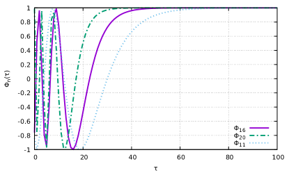
Figure 1: Sample basis elements utilized throught this work. Note how they allow for highly oscillatory behavior at small values of the triad and then smoothen out as the values get larger.

The basis function method ultimately involves solving a linear system of equations for a vector of weights $\omega_{n}$, where $n$ is an index spanning the number of basis elements. The system matrix is represented as an “interpolation matrix”, with each entry being the sequence in Eqn. 7, and with each $B$ replaced with an appropriate representation of Eqn. 8. Each row in this matrix corresponds to an increasing value of $\tau$ in the domain of the computation. Thus, Eqn. 7 would be represented as

$$\sum^{N}_{n=0}\omega_{n}\big{[}(\sqrt{|\tau|}+\sqrt{|\tau+2\delta_{c}|})\Phi_{n}(\tau+2\delta_{c})$$

$$-(\sqrt{|\tau|}+\sqrt{|\tau-2\delta_{c}|})\Phi_{n}(\tau-2\delta_{c})$$

$$+\lambda(\sqrt{|\tau+\delta_{c}|}-\sqrt{|\tau-\delta_{c}|})\Phi_{n}(\tau)\big{]}=0$$ (9)

To solve the above system for the function $B(\tau)$, other than the trivial $B(\tau)=0$, inspiration was taken from a standard technique for numerically solving partial differential equations. A row can be injected into the system matrix, as long as there is an accompanying column, to disrupt the homogeneity of the system without fundamentally changing the computation. This row can be interpreted as numerically incorporating initial or boundary conditions; and in our approach is treated as a restriction on the solution. For our results in this section, we used $\sum_{n}\omega_{n}\Phi_{n}(\tau=T)=1$ for a large value of $T$.

Using this approach, a reconstructed solution can be generated, which is in precise agreement with the recursively computed solution. In Fig. 2 we show a sample basis solution for the $B(\tau)$ equation as compared with a recursion based solution computed by stepping through the values of the $\tau$ variable. There, we set $\gamma\delta_{b}\rightarrow 0$ (a requirement for stable solutions) and set $\delta_{c}=2\delta_{b}=\lambda=1$ for simplicity.

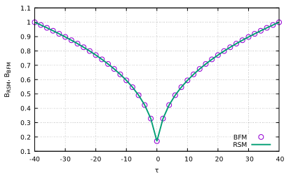
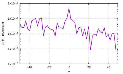
Figure 2: Solution of the $B(\tau)$ equation using the basis function method as compared with a solution computed by stepping through the $\tau$ values using a recursive approach. The upper panel shows both solutions plotted together. The lower panel depicts the absolute difference between the two solutions, which is on the scale of machine precision.

Similarly to solve Eqn. 6 we first make the substitution $C(\mu)\equiv A(\mu+2\delta_{b})-A(\mu-2\delta_{b})$ which results in

$$\mu\big{(}C(\mu+2\delta_{b})-C(\mu-2\delta_{b})\big{)} +$$

$$2\delta_{b}\big{(}C(\mu+2\delta_{b})+C(\mu-2\delta_{b})\big{)} = -2\lambda C(\mu)~{}.$$ (10)

This allows us to easily solve Eqn. 6 using both the basis function method and the recursive approach. The outcome is similar as that shown previously for the $B(\tau)$ function.

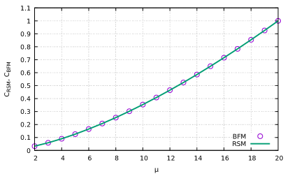
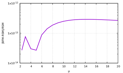
Figure 3: Solution of the $C(\mu)$ equation using the basis function method as compared with a solution computed by stepping through the $\mu$ values using a recursive approach. The upper panel shows both solutions plotted together. The lower panel depicts the absolute difference between the two solutions.

III.2 Full 2D Solution: Evolution with Basis Functions

The numerical solution computation for the full 2D non-separable case, takes a similar approach. The solution is again taken to be a weighted-sum of the basis functions Eqn. 8, but with $\tau$ dependent weights. This leads to Eqn. II taking the form

$$\sum^{N}_{n=0}\omega_{n}(\tau-2\delta_{c})(\Phi_{n}(\mu+2\delta_{b})-\Phi_{n}(\mu-2\delta_{b}))=$$

$$\hskip-5.69046pt\tfrac{\sqrt{|\tau|}+\sqrt{|\tau+2\delta_{c}|}}{\sqrt{|\tau|}+\sqrt{|\tau-2\delta_{c}|}}\left(\Psi_{\mu+2\delta_{b},\tau+2\delta_{c}}-\Psi_{\mu-2\delta_{b},\tau+2\delta_{c}}\right)$$

$$\hskip-5.69046pt+\tfrac{1}{2\delta_{b}}\,\tfrac{\sqrt{|\tau+\delta_{c}|}-\sqrt{|\tau-\delta_{c}|}}{\sqrt{|\tau|}+\sqrt{|\tau-2\delta_{c}|}}\bigg{[}(\mu+2\delta_{b})\Psi_{\mu+4\delta_{b},\tau}+$$

$$\hskip 11.38092pt(\mu-2\delta_{b})\Psi_{\mu-4\delta_{b},\tau}-2\mu(1+2\gamma^{2}\delta_{b}^{2})\Psi_{\mu,\tau}\bigg{]}~{}.$$ (11)

The solution can then be reconstructed on the full range of $\mu,\tau$ values via

$$\Psi_{\mu,\tau}=\sum^{N}_{n=0}\omega_{n}(\tau)\Phi_{n}(\mu)~{}.$$ (12)

The $\tau$ dependence is captured by stepping through a $\tau$-valued grid of this reconstructed solution.

Similar to the 1D variable-separated case, the basis function method ultimately leads to a linear system of equations. The system involves finding the weights $\omega_{n}$, while the invertible system matrix represents the left-hand-side of Eqn. III.2. A boundary condition is implemented in the manner of row-column injection used previously, where $\lim_{\mu\rightarrow\infty}\Psi_{\mu,\tau}=0$ is represented as $\sum_{n}\omega_{n}\Phi_{n}(\mu=M)=0$. As typically done in such models, we impose a constraint that represents an initial “semi-classical” wave-packet, i.e. a Gaussian profile for the solution at large $\tau$, and then step backwards in $\tau$, ultimately evolving the system deep into the quantum regime and beyond.

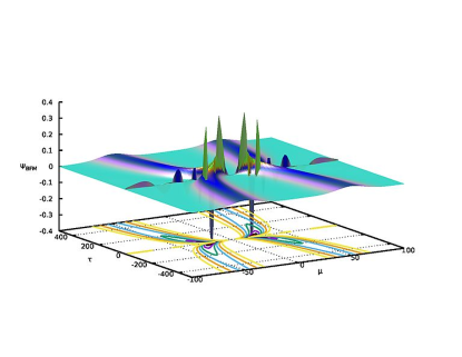
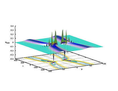
Figure 4: Solution of Eqn. II using the basis function method (upper panel) as compared with a solution computed by stepping through the $\tau,\mu$ values using a recursive approach (lower panel).

The error denoted by the $L_{\infty}$-norm as the maximum value of the residual between the recursive step method and basis method solutions at slices of constant $\tau$ is depicted in Fig. 5.

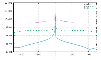
Figure 5: $L_{\infty}$-norm of the error at each value of $\tau$ for different number of basis elements $N=20,23,25$.

It is clear that the error stays low for the larger values of $\tau$, however it increases in the neighborhood of $\tau=0$. This is likely due to the use of a relatively small number of basis elements. In fact, as seen in Fig. 5, it is clear that overall error reduces dramatically with even a modest increase in the number of basis elements. Of course, one can also envision a minor tweak in the form of the basis to reduce the error in the small $\tau$ regime further. We do not attempt to do that in this work.

The agreement between the basis and recursive method can be even further inspected by examining the volume expectation value $\langle v\rangle$. This is shown in Fig. 6.

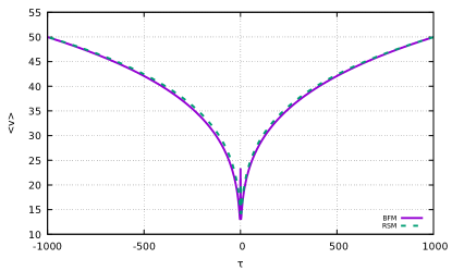
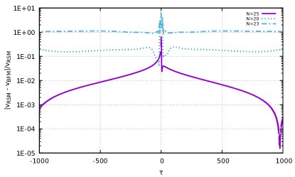
Figure 6: $\langle v\rangle$ computed using both the basis function method and the recursive step method, and the associated relative difference.

III.2.1 Optimization

To reduce computational cost, we make use of a key property of the solutions, i.e. they must get smoother for the larger triad values. When the solutions are smooth, they can be interpolated very effectively, thus allowing for a significant reduction in the “sampling rate”. In order to take advantage of this, we only solve over a subset of triad values as computed through this expression

$$\mu_{i+1}=\mu_{i}+\lfloor 1+\big{(}\frac{2\mu_{i}}{25}\big{)}^{2}\rfloor$$ (13)

where $\lfloor\rfloor$ denotes the “integer part” or the gint function. Visually, this set can be represented as shown in Fig. 7. Through some experimentation, we discovered that this form yields significant computational benefit with relatively little loss of accuracy. This allows us to reduce the effective grid size by a factor of 10, offering us a tremendous speed-up!

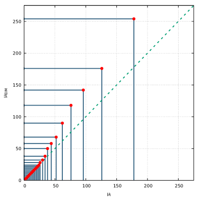
Figure 7: Subset of $\mu$ variable grid values compared with optimal $\mu$ variable grid values obtained through the empirical interpolation method.

In addition, while the choice of basis etc. was made largely based on physical considerations and numerical experimentation, we can show that this choice is reasonably optimal using a reduced basis approach BasReduc2010 with an empirical interpolation method framework EIM2008 , calculated via the greedy algorithm AFHNT13 . This was done using the open source code rompy rompy1 ; rompy2 which demonstrated that the optimal sampling nodes have a similar distribution to the nodes generated with Eqn. 13. This is shown graphically in Fig. 7. Utilizing the chosen basis function in Eqn. 8, one can generate an associated Vandermonde matrix, with the elements

$$V_{i,j}=\Phi_{j}(\mu_{i})~{}.$$ (14)

If the basis elements $\Phi_{j}(\mu_{i})$ are considered as a reduced basis, one can then perform a singular value decomposition (SVD) of $V_{i,j}$. This demonstrates that the chosen basis is approximately orthonormal and well-conditioned. This was further verified by performing Gram-Schmidt orthonormalization on the basis, which led to no perceived difference in the orthogonality of the basis, and only an insignificant reduction in the conditioning. Thus, we observe that while certain techniques may be used to improve our basis function method (e.g. Gram-Schmidt, Empirical Interpolation), they are not necessarily required.

III.3 Instability

After performing von-Neumann stability analysis on Eqn. II, it was noted previously YKS that the model is subject to an instability condition,

$$\mu > 4\tau~{}.$$ (15)

This condition $\mu>4\tau$ is of particular interest as it only appears through use of von-Neumann stability analysis in the context of the full 2D system Eqn. II, and not in the variable-separable case. This is indicative of the fact that the $\mu>4\tau$ condition is a consequence of the full 2D form of the quantum Hamiltonian constraint. In this section, we attempt to understand how exactly this instability appears in the 2D equation – both, in the context of the stencil-based, finite-difference-like stepping approach and, of course, the basis function method.

III.3.1 The Large $\mu,\tau$ Limit

Beginning with the original Eqn. II and taking the approximation $(\mu,\tau)>>(\delta_{b},\delta_{c})$ and setting $\gamma\delta_{b}\rightarrow 0$, we obtain

$$(1+\sqrt{|1+2\frac{\delta_{c}}{\tau}|})\left(\Psi_{\mu+2\delta_{b},\tau+2\delta_{c}}-\Psi_{\mu-2\delta_{b},\tau+2\delta_{c}}\right)$$

$$\hskip-5.69046pt+\tfrac{1}{2\delta_{b}}\,(\sqrt{|1+\frac{\delta_{c}}{\tau}|}-\sqrt{|1-\frac{\delta_{c}}{\tau}|})\bigg{[}(\mu)\Psi_{\mu+4\delta_{b},\tau}+$$

$$\hskip 11.38092pt(\mu)\Psi_{\mu-4\delta_{b},\tau}-2\mu\Psi_{\mu,\tau}\bigg{]}+$$

$$\hskip-5.69046pt(1+\sqrt{|1-2\frac{\delta_{c}|}{\tau}})\left(\Psi_{\mu-2\delta_{b},\tau-2\delta_{c}}-\Psi_{\mu+2\delta_{b},\tau-2\delta_{c}}\right)$$

$$=0~{}.$$ (16)

Next, we insert the following Taylor approximation, making implicit use of the expectation that the solution tends towards smooth behavior for large values of $\mu,\tau$

$$\Psi_{\mu\pm l\delta_{b},\tau\pm m\delta_{c}}\approx \Psi(\mu\pm l\delta_{b},\tau\pm m\delta_{c})$$

$$\rightarrow \Psi\pm l\delta_{b}\tfrac{\partial}{\partial\mu}\Psi\pm m\delta_{c}\tfrac{\partial}{\partial\tau}\Psi$$

$$+\tfrac{(l\delta_{b})^{2}\partial^{2}}{2!\partial\mu^{2}}\Psi+\tfrac{(m\delta_{c})^{2}\partial^{2}}{2!\partial\tau^{2}}\Psi$$

$$\pm 2lm\delta_{b}\delta_{c}\tfrac{\partial^{2}}{\partial\mu\partial\tau}\Psi+\dots$$

$$\sqrt{|1\pm 2\frac{\delta_{c}}{\tau}|}\approx 1\pm\frac{\delta_{c}}{\tau}~{}.$$

This substitution reduces Eqn. III.3.1, to the expression

$$4\tau\frac{\partial^{2}}{\partial\mu\partial\tau}\Psi+\frac{\partial}{\partial\mu}\Psi+\mu\frac{\partial^{2}}{\partial\mu^{2}}\Psi=0$$ (17)

which can be further reduced into an equation of the form of the advection partial differential equation,

$$\dot{\beta}+\frac{\mu}{4\tau}\beta^{\prime}=0$$

$$\beta\equiv\mu\frac{\partial}{\partial\mu}\Psi~{}.$$ (18)

Now, it is relatively easy to see why an instability appears for $\mu>4\tau$ part of the computational domain. Making an analogy with the so-called, “CFL condition” cfl that commonly appears in numerical partial differential equation methods, Eqn. III.3.1 presents an advection equation with a locally defined speed of $v=\tfrac{\mu}{4\tau}$. This defines, at each point in ($\tau,\mu$), a local light cone extending into the past defined by the region traced out by the characteristic speed $v$. However, the finite-difference stencil as defined by the Hamiltonian constraint, has a triad stepping ratio of $\delta_{b}/2\delta_{c}=1$. This results in an instability when $v>1$, since the local physical domain of dependence is no longer fully contained within the local computational domain as determined by the quantum Hamiltonian constraint.

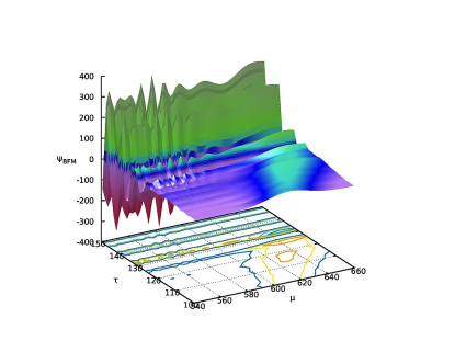
Figure 8: Evolution using the basis function method into the unstable regime of $\mu,\tau$.

As mentioned before, the instability condition of $\mu>4\tau$ is a result of recursive stepping through both $\mu$ and $\tau$ as in Eqn. II. With a global method like the basis method, it could be reasoned that such a local instability condition may be avoided. However, it does not; this can be seen by performing a “shift” of coordinates, $\mu\rightarrow\mu+555,\tau\rightarrow\tau+100$ and allowing part of the Gaussian wavepacket to evolve into the unstable regime. Fig. 8 depicts such a sample evolution.

We find that the instability condition as shown is still applicable even in the basis function method. It is suspected that this is due to an intrinsic issue with the CS model, or perhaps due to the lack of a complete Hilbert space of solutions or possibly even a reflection of some underlying physics. Thus, von-Neumann analysis continues to be beneficial towards providing insight on the viability of models in loop quantum cosmology. More specifically, it is able to provide various constraints on such models based on the requirement that evolutions must be stable nlqc ; YKS ; SS .

III.3.2 Stability in the Basis Function Method

To understand the instability in the context of the basis function approach, we take Eqns. II and 12 together, while noting that the only time-varying component in Eqn. 12 is $\vec{\omega}$. We then rewrite Eqn. II using vector and matrix notation

$$\Psi_{\mu\pm k\delta_{b},\tau\pm n\delta_{c}}\rightarrow \sum^{N}_{i=0}\Phi_{i}(\mu\pm k\delta_{b})\omega_{i}(\tau\pm n\delta_{c})$$

$$= \mathbf{\Phi}(\mu\pm k\delta_{b})\vec{\omega}_{\tau\pm n\delta_{c}}~{}.$$ (19)

where $\mathbf{\Phi}$ is a square matrix with the different basis elements arranged in columns and each row representing a different $\mu$ value. In this notation the CS model can be rewritten as

$$\big{(}\tfrac{\sqrt{|\tau|}+\sqrt{|\tau-2\delta_{c}|}}{\sqrt{|\tau|}+\sqrt{|\tau+2\delta_{c}|}}\big{)}\bigg{[}\mathbf{\Phi}(\mu-2\delta_{b})-\mathbf{\Phi}(\mu+2\delta_{b})\bigg{]}\vec{\omega}_{\tau-2\delta_{c}}$$

$$\hskip-5.69046pt+\frac{1}{2}\big{(}\tfrac{\sqrt{|\tau+\delta_{c}|}-\sqrt{|\tau-\delta_{c}|}}{\sqrt{|\tau|}+\sqrt{|\tau+2\delta_{c}|}}\big{)}\bigg{[}(\mu+2\delta_{b})\mathbf{\Phi}(\mu+4\delta_{b})+(\mu-2\delta_{b})\mathbf{\Phi}(\mu-4\delta_{b})-2\mu\mathbf{\Phi}(\mu)\bigg{]}\vec{\omega}_{\tau}$$

$$\hskip-5.69046pt-\bigg{[}\mathbf{\Phi}(\mu-2\delta_{b})-\mathbf{\Phi}(\mu+2\delta_{b})\bigg{]}\vec{\omega}_{\tau+2\delta_{c}}=\vec{0}~{}.$$ (20)

Given that $\mathbf{\Phi}$ is a matrix of full rank, we can compute the inverse of matrix $\mathbf{A}$ (defined below) and obtain

$$\mathbf{I}\vec{\omega}_{\tau+2\delta_{c}}+\frac{1}{2}\big{(}\tfrac{\sqrt{|\tau-\delta_{c}|}-\sqrt{|\tau+\delta_{c}|}}{\sqrt{|\tau|}+\sqrt{|\tau+2\delta_{c}|}}\big{)}\mathbf{A}^{-1}\mathbf{B}\vec{\omega}_{\tau}-\big{(}\tfrac{\sqrt{|\tau|}+\sqrt{|\tau-2\delta_{c}|}}{\sqrt{|\tau|}+\sqrt{|\tau+2\delta_{c}|}}\big{)}\mathbf{I}\vec{\omega}_{\tau-2\delta_{c}}= \;\vec{0}$$

$$\mathbf{\Phi}(\mu-2\delta_{b})-\mathbf{\Phi}(\mu+2\delta_{b})\equiv \;\mathbf{A}$$

$$\big{[}(\mu+2\delta_{b})\mathbf{\Phi}(\mu+4\delta_{b})+(\mu-2\delta_{b})\mathbf{\Phi}(\mu-4\delta_{b})-2\mu\mathbf{\Phi}(\mu)\big{]}\equiv \;\mathbf{B}~{}.$$ (21)

This can be further reduced down to

$$\mathbf{I}\vec{\omega}_{\tau+2\delta_{c}}+\frac{1}{2}\alpha\mathbf{D}\vec{\omega}_{\tau}-\beta\mathbf{I}\vec{\omega}_{\tau-2\delta_{c}}= \vec{0}$$

$$\mathbf{D}\equiv\;\mathbf{A}^{-1}\mathbf{B}$$

$$\alpha\equiv\big{(}\tfrac{\sqrt{|\tau-\delta_{c}|}-\sqrt{|\tau+\delta_{c}|}}{\sqrt{|\tau|}+\sqrt{|\tau+2\delta_{c}|}}\big{)}$$

$$\beta\equiv\big{(}\tfrac{\sqrt{|\tau|}+\sqrt{|\tau-2\delta_{c}|}}{\sqrt{|\tau|}+\sqrt{|\tau+2\delta_{c}|}}\big{)} ~{}.$$ (22)

Finally, if the following definitions are made,

$$\vec{q}_{\tau}\equiv\begin{bmatrix}\vec{\omega}_{\tau}\\ \vec{\omega}_{\tau-2\delta_{c}}\end{bmatrix} \mathbf{\Pi}\equiv\begin{bmatrix}-\tfrac{1}{2}\alpha\mathbf{D}&\beta\mathbf{I}\\ \mathbf{I}&\mathbf{0}\end{bmatrix}$$ (23)

then one can use Eqn. 23 to express Eqn. III.3.2 in the following manner,

$$\vec{q}_{\tau+2\delta_{c}}=\mathbf{\Pi}\vec{q}_{\tau}~{}.$$ (24)

Now, we use the eigenvalues of matrix $\mathbf{\Pi}$ to test for stability; if any of the eigenvalue magnitudes exceed unity, that makes the solution of Eqn. 24 grow unboundedly. With some additional simplifications (in particular, $(\mu,\tau)>>(\delta_{b},\delta_{c})$) accompanied with some numerical computations it is not difficult to see that one obtains the same unstable region ($\mu>4\tau$) as derived before in Ref. YKS using basic von Neumann stability analysis.

IV Discussion and Conclusions

In this paper, we have developed a new numerical method that is particularly suitable for computing solutions to the quantum Hamiltonian constraint of models in loop quantum cosmology. The method is inspired by the spectral collocation method that is commonly used for numerically solving partial differential equations. It uses a special set of basis functions that take full advantage of the expected behavior of physical solutions of the model. We also compared the new basis function method with the previously used approach of a stencil-style computation using a recursive computation over a grid of allowed values for the triad variables. In addition, we also discussed how the stability analysis appears in the context of the basis approach.

In this section we will document how the basis function method improves upon previous approaches. As pointed out earlier, the main advantage is computational efficiency and ease of parallelization.

IV.1 Parallelizability

The basis function method ultimately involves the computation of a solution of a linear system of equations of size proportional to the square of the number of basis elements in use. Since this is a very well-studied problem, there exist many highly optimized solvers available even for parallel hardware such as multi-core CPUs and many-core GPUs. On the other hand, the recursive step method is intrinsically serial and rather challenging to parallelize.

Cores	BFM Run-Time (s)
1	161.110
2	85.805
4	48.852
8	29.751

Table 1: Run-Time by number of cores with simple OpenMP multi-threading on $\mu,\tau\in[-1600,1600]$ grid

With a simple multi-threaded implementation for the BFM algorithm, the benefit of parallelization can be clearly seen. Increased benefit is expected when the number of basis elements gets larger; and we anticipate a more in-depth study of this feature for both multi-core CPUs and many-core GPUs in future work.

IV.2 Precision

As mentioned above, the basis function method involves solving a linear system of equations. Performing an analysis on the backward error of matrix inversion techniques yields

$$\mathbf{A}\vec{x}= \vec{b}$$

$$\epsilon_{BFM}=||\mathbf{A}^{-1}\vec{b}-\vec{x}||= \mathcal{O}(\kappa_{2}\epsilon_{machine})$$

$$\kappa_{2}\equiv ||\mathbf{A}^{-1}||_{2}||\mathbf{A}||_{2}\propto N~{}.$$ (25)

On the other hand it has been found that for a recursive step method with $\mu\in[\tfrac{-M}{2},\tfrac{M}{2}]$ and $\tau\in[\tfrac{-T}{2},\tfrac{T}{2}]$, the error $\epsilon_{RSM}\propto\mathcal{O}(T\times M\epsilon_{machine})$. Since standard backward error is proportional to the number of basis elements, we have shown that a small and constant number can compute solutions on a range of domains accurately; it stands to reason that as long as the non-zero regions of the computed solution are reasonably well sampled by the basis, the BFM approach can calculate a larger range of solutions with a set level of computational precision.

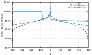
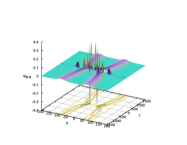
Figure 9: Relative $L_{2}$ error for various size domains, and evolution with the basis function method over large domain, $\mu,\tau\in[-1600:1600]$

It can be seen in Fig. 9 that the recursive step method based solution experiences unbounded growth due to fixed, finite available precision; while the basis method computed solution maintains the correct overall behavior expected. For a closer analysis of the effects that finite precision can have on the recursive step method solutions a precision test can be performed. For such a test, we maintain a constant domain and solve identical simulations with varying precision. The error can then be analyzed by taking the highest precision solution as most accurate. Our standard error analysis follows as

$$\epsilon_{P}(\tau_{i}) =\frac{\sum_{n}|\Psi_{Quad}(\mu_{n},\tau_{i})-\Psi_{P}(\mu_{n},\tau_{i})|^{2}}{\sum_{n}\Psi^{2}_{Quad}(\mu_{n},\tau_{i})}$$

where $P$ is a precision other than quadruple-precision (e.g. double, single). The results are depicted in Fig. 10. They suggest that the recursive step method is far more prone to suffer from precision limitations over the basis method. This ultimately translates into a major computational advantage in favor of the basis method.

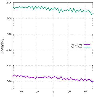
Figure 10: Precision test for single (4-byte), and double (8-byte) precision. It is clear that error grows significantly as the evolution progresses (recall, the system evolves backward in $\tau$).

In summary, we have developed a new numerical approach towards solving quantum Hamiltonian constraints in loop quantum cosmology. The approach makes use of a set of basis functions, specifically designed using key physical features of the solutions in mind. This basis method, borrows from the well-known spectral collocation method for solving partial differential equations. We demonstrate the efficacy of the method and compare it with the previously used recursive step method. We find that the basis method offers a number of benefits over the previously used approach, especially in the area of computational efficiency. Throughout this paper, we use the Corichi and Singh loop quantum model of the Schwarzschild interior for demonstration purposes.

Acknowledgements: The authors would like to thank Drs. Alfa Heryudono, Scott Field and Sigal Gottlieb for very helpful suggestions throughout this work. G. K. thanks research support from National Science Foundation (NSF) Grant No. PHY-1701284 and Office of Naval Research/Defense University Research Instrumentation Program (ONR/ DURIP) Grant No. N00014181255.

References

- (1) T. Thiemann, Modern Canonical Quantum General Relativity, Cambridge Monographs on Mathematical Physics, Cambridge University Press (2008).
- (2) C. Rovelli, Quantum Gravity, Cambridge University Press (2007).
- (3) A. Ashtekar, J. Pullin, Loop Quantum Gravity: The First 30 Years (100 Years of General Relativity), World Scientific (2017).
- (4) A. Ashtekar, and P. Singh, Class. Quant. Grav. 28, 213001 (2012).
- (5) M. Bojowald, Living Rev. Rel., 11, 4 (2008).
- (6) A. Ashtekar, T. Pawlowski, and P. Singh, Phys. Rev. Lett. 96, 141301 (2006).
- (7) A. Ashtekar, T. Pawlowski, and P. Singh, Phys. Rev. D 74, 084003 (2006).
- (8) P. Singh, Computing in Science & Engineering 20(4), 26 (2018).
- (9) D. Brizuela, D. Cartin, and G. Khanna, SIGMA 8, 001 (2012).
- (10) P. Singh, Class. Quant. Grav. vol. 29, 244002 (2012).
- (11) P. Diener, B. Gupt, M. Megevand, and P. Singh, Class.Quant. Grav., 31, 165006 (2014)
- (12) A. Corichi, P. Singh, Class. Quantum Grav. 33, 055006 (2016).
- (13) A. Yonika, G. Khanna, P. Singh, Class. Quantum Grav. 35, 045007 (2018).
- (14) H. Haggard and C. Rovelli, Phys. Rev. D 92, 104020 (2015).
- (15) E. Bianchi, M. Christodoulou, F. D’Ambrosio, H. Haggard and C. Rovelli, Class. Quantum Grav. 35, 225003 (2018).
- (16) J. Olmedo, S. Saini and P. Singh, Class. Quantum Grav. 34, 225011 (2017).
- (17) S. Connors, G. Khanna, Class. Quantum Grav. 23, 2919 (2006).
- (18) S. Chaturantabut, D. Sorensen, SIAM J. of Sci. Comput. 32(5), (2010)
- (19) Y. Maday, N. Nguyen, A. Patera, G. Pau, Communications on Pure and Applied Analysis 8(1), (2009)
- (20) H. Antil, S. Field, F. Herrmann, R. Nochetto, M. Tiglio, Journal of Scientific Computing 57, (2013)
- (21) S. Field, C. Galley, J. Hesthaven, J. Kaye, M. Tiglio, Phys. Rev. X 4, 031006 (2014)
-
(22)
C. Galley, rompy package
https://bitbucket.org/chadgalley/rompy/src/master - (23) R. Courant, K. O. Friedrichs, H. Lewy, IBM Journal 11, 215 (1967).
- (24) P. Diener, B. Gupt and P. Singh, Class. Quant. Grav. 31, 025013 (2014)
- (25) S. Saini and P. Singh, Class. Quant. Grav. 36, 105010 (2019)