Recommender Systems with Heterogeneous Side Information

Abstract.

In modern recommender systems, both users and items are associated with rich side information, which can help understand users and items. Such information is typically heterogeneous and can be roughly categorized into flat and hierarchical side information. While side information has been proved to be valuable, the majority of existing systems have exploited either only flat side information or only hierarchical side information due to the challenges brought by the heterogeneity. In this paper, we investigate the problem of exploiting heterogeneous side information for recommendations. Specifically, we propose a novel framework jointly captures flat and hierarchical side information with mathematical coherence. We demonstrate the effectiveness of the proposed framework via extensive experiments on various real-world datasets. Empirical results show that our approach is able to lead a significant performance gain over the state-of-the-art methods.

1. Introduction

Recommender systems can mitigate the information overload problem by providing online users with the most relevant information (Sarwar et al., 2001; Su and Khoshgoftaar, 2009; Ricci et al., 2015). A successful recommender system often requires accurate understanding of user preferences. Collaborative filtering, which models the interactions between users and items, is one of the most popular techniques to achieve this goal (Sarwar et al., 2001; Koren et al., 2009; He et al., 2017). Traditional collaborative filtering based recommender systems have been proven to be suffered from the data sparsity and cold-start problems (Adomavicius and Tuzhilin, 2005; Su and Khoshgoftaar, 2009). On the other hand, in addition to interactions, users and items are often associated with side information, which has become increasingly available in real-world recommender systems (Fang and Si, 2011; Ning and Karypis, 2012). Such side information provides independent sources for recommendations, which can mitigate the data sparsity and cold start problems and have great potentials to boost the performance. As a consequence, a large body of research has been developed to exploit side information for recommendations (Yang et al., 2016; Lu et al., 2012; Ricci et al., 2015; Wang et al., 2018).

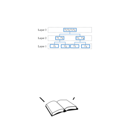
Figure 1. An illustration of flat and hierarchical side information.

Side information is typically heterogeneous, which can be roughly categorized into flat and hierarchical side information (Wang et al., 2018). Flat and hierarchical side information are referred to attributes associated with users and items presenting no hierarchical and hierarchical structures, respectively (Wang et al., 2018). Take books for example, side information of one book can include the publish year, the book authors, the written language, and the genres it belongs to. Attributes such as year, author and language, presenting no hierarchical structures, are flat. The genres, however, contain subtypeOf relationship and can be organized in a hierarchical structure. Figure 1 gives a concrete example, which shows six attributes of the book Animal Farm with colored background. The flat information includes George Orwell, 1945 and English and are listed in the left part of figure. Literature&Fiction, Historical Fiction, and Political are the genres Animal Farm belongs to according to Amazon Web Store. As shown in the figure, these genres are organized into a hierarchical structure as genre$\rightarrow$subgenre$\rightarrow$detailed-genre such that Animal Farm firstly belongs to the genre Literature&Fiction, under which there are sub-genres such as Historical Fiction and Genre Fiction. In this sub-genre level, Animal Farm belongs to Historical Fiction. It further falls into a more detailed-category Political. Likewise, users are also associated with both flat information such as age, gender, education level and hierarchical information such as communities they belong to and the places of their birth.

There are numerous works incorporating flat or hierarchical side information for recommendations  (Fang and Si, 2011; Ning and Karypis, 2012; Yang et al., 2016; Lu et al., 2012; Ricci et al., 2015; Wang et al., 2018). Most of these systems have been designed to exploit either only flat side information or only hierarchical side information. The major reason is that flat and structured side information are intrinsically different and it is challenging to jointly exploit them. One trivial solution is to flatten the hierarchy and treat it as flat information. However, such solution ignores the unique properties of hierarchical information, which have been proven beneficial by previous works (Lu et al., 2012; Wang et al., 2018; Menon et al., 2011). In fact, both flat and hierarchical side information can provide valuable information for understanding user preferences and item characteristics. For instance, female are generally more interested in high heel shoes than male and items belonging to the same detailed-genre are likely to be more similar than those in the same sub-genre. Thus, it is desired to design frameworks incorporating the two types of side information simultaneously.

In this paper, we investigate the problem of exploiting both flat and hierarchical side information for recommendations. We propose a novel framework, which aims to address two challenges: (1) how to jointly capture heterogeneous side information and (2) how to mathematically use them for recommendations. The main contributions of our work can be summarized as follows:

• We provide a principled approach to simultaneously capture both flat and hierarchical information mathematically.

• We introduce a unified recommendation framework HIRE, which can model Heterogeneous side Information for REcommendation coherently.

• We conduct extensive experiments with various real-world datasets to validate the effectiveness of the proposed framework and understand the importance of flat and hierarchical side information for recommendations.

2. Methodology

In this section, we present the proposed recommendation framework that coherently captures flat and hierarchical information of both users and items. Specifically, we firstly introduce the notations that will be used in the rest of the paper and then describe a basic model which forms the basis of the framework. After that, we go into details of the framework components that model the flat and heterogeneous information, respectively, combining of which leads to an optimization problem. Finally, we propose an efficient algorithm to solve it.

Throughout this paper, regular letters are used to denote scalers. The vectors and matrices are represented by bold lower-case letters such as ${\bf h}$ and bold upper-case letters such as W, respectively. In addition, for an arbitrary matrix ${\bf W}$, we use ${\bf W}(i,:)$ and ${\bf W}(:,j)$ to denote the $i^{th}$ row and $j^{th}$ column of it, respectively; and the $(i,j)^{th}$ entry of ${\bf W}$ is represented as ${\bf W}(i,j)$. The transpose and Frobenius norm of ${\bf W}$ is denoted as ${\bf W}^{T}$ and $\|{\bf W}\|_{F}^{2}$, respectively. Moreover, let $\mathcal{U}=\{u_{1},u_{2},\cdots,u_{n}\}$ to be the set of $n$ users and $\mathcal{V}=\{v_{1},v_{2},\cdots,v_{m}\}$ be the set of $m$ items. We assume there exists a user-item rating matrix ${\bf R}\in\mathbb{R}^{n\times m}$ and if a user $u_{i}$ has rated item $v_{j}$, ${\bf R}(i,j)>0$ denotes the rating score, otherwise, ${\bf R}(i,j)=0$. In addition, let ${\bf X}\in\mathbb{R}^{d_{x}\times n}$ and ${\bf Y}\in\mathbb{R}^{d_{y}\times m}$ be the matrices that contain flat side information of users and items with $d_{x}$ and $d_{y}$ associated attributes, respectively. Next, we will describe a basic recommendation model, based on which we will build the whole framework.

2.1. The Basic Model

Weighted matrix factorization is an effective approach used in collaborative filtering based recommender systems to obtain users’ and items’ representations that contain information regarding users’ preference and items’ characteristics. Specifically, it decomposes the rating matrix and models the users and items in the same low-dimensional latent space. Mathematically, weighted matrix factorization solves the following optimization problem:

$$\min_{{\bf U},{\bf V}}\underbrace{\|{\bf M}\odot({\bf R}-{\bf U}{\bf V})\|^{2}_{F}+\lambda(\|{\bf U}\|^{2}_{F}+\|{\bf V}\|^{2}_{F})}_{f({\bf U},{\bf V})}$$

where $\odot$ is the Hadamard operation denoting element-wise multiplication. ${\bf M}\in\mathbb{R}^{n\times m}$ is the indication matrix such that ${\bf M}(i,j)=1$ if ${\bf R}(i,j)>0$, otherwise, ${\bf M}(i,j)=0$. The obtained matrices ${\bf U}\in\mathbb{R}^{n\times d}$ and ${\bf V}\in\mathbb{R}^{d\times m}$ are the corresponding representations of users and items in the latent space. Thus, the rating score given by $u_{i}$ to $v_{j}$ is approximated by the dot item of their latent representations, that are ${\bf U}(i,:)$ and ${\bf V}(:,j)$, respectively. $\lambda$ is used to control the weight of regularization terms that are adopted to avoid overfitting. One of the most important strength of matrix factorization based model is that it allows to incorporate other information in addition to the ratings (Koren et al., 2009). Next, we will base on the basic weighted matrix factorization model to build our framework.

2.2. Capturing The Flat Information

The side information of items or users are intrinsically heterogeneous, which can be flat and heterogeneous. For example, in Figure 1, a book can have both flat attributes such as author, year, and hierarchical attributes such as genres it belongs to. The difference between different types of side information requires special treatment for each individual. In this subsection, we describe the model component that aims to capture the flat side information. To simplify, we first focus on capturing side information of users and then generalize it to that of items.

In weighted matrix factorization, users’ latent representation matrix ${\bf U}$ contains their preference indicated by the rating scores they give to items. The side information, however, provides another independent source from which users’ preference could be inferred. For example, it is very likely that a programmer is more interested in a mechanical keyboard than a dancer, which suggests that users’ occupation could provide an important indicator whether an item should be recommended or not. In addition, both hidden representation ${\bf U}(i,:)$ and side information ${\bf X}(:,i)$ describe the same user $u_{i}$. Hence, in the same latent space, ${\bf U}(i,:)$ and ${\bf X}(:,i)$ should be similar. With this intuition, we extend the basic weight matrix factorization model to capture the flat side information contained in ${\bf X}$ as follows:

$$\min_{{\bf U},{\bf V}} f({\bf U},{\bf V})+\gamma\|{\bf S}^{u}{\bf U}^{T}-{\bf X}\|^{2}_{F}$$

where ${\bf S}^{u}\in\mathbb{R}^{d_{x}\times d}$ is the projection matrix that projects users’ hidden representations ${\bf U}$ into the same latent space as ${\bf X}$. The Frobenius norm indicates the distance between the representations of users from two perspectives, which are forced to be close. In this way, the learned users representations ${\bf U}$ also capture flat side information contained in ${\bf X}$.

However, in practice, ${\bf X}$ is usually very sparse. For example, while a user profile could include various types of information, making ${\bf X}$ high-dimensional, many users may only provide a part of the profile, which renders ${\bf X}$ very sparse. To address this issue, we adopt autoencoders, which provide a way to obtain robust feature representations in an unsupervised manner (Bengio et al., 2013) and have been successfully applied in various tasks such as speech enhancement (Lu et al., 2013), natural language generation (Li et al., 2015b) and face alignment (Zhang et al., 2014). In this work, we choose to incorporate marginalized denoising autoencoders (MDA) into the proposed model, as it is much more computationally efficient than others (Chen et al., 2012) and we leave incorporating other autoencoders as one future direction.

MDA firstly takes the side information ${\bf X}=[{\bf x}_{1},{\bf x}_{2},\cdots,{\bf x}_{n}]$ as input and corrupts the features to obtain noising version ${\tilde{\bf x}}_{i}$ for each user $u_{i}$. The corruption process can be done in different ways. In this paper, we follow the practice in (Chen et al., 2012) and corrupt features by randomly setting each feature to be $0$ with the probability $p\geq 0$. In contrast to traditional stacked denoising autoencoders that have the two-level encoder and decoder structures, in MDA, only one single mapping ${\bf W}^{u}:\mathbb{R}^{d_{x}}\rightarrow\mathbb{R}^{d_{x}}$ is used to reconstruct the original features and the reconstruction loss is defined as follows:

(1) $$\mathcal{L}({\bf W}^{u})=\frac{1}{2n}\sum_{i=1}^{n}\|{\bf x}_{i}-{\bf W}^{u}{\tilde{\bf x}}_{i}\|^{2}$$

The random corruption of the features may lead to the solution ${\bf W}^{u}$ of high variance. In order to avoid this, $k$-times corruption is performed and the overall reconstruction loss becomes:

(2) $$\mathcal{L}({\bf W}^{u})=\frac{1}{2nk}\sum_{j=1}^{k}\sum_{i=1}^{n}\|{\bf x}_{i}-{\bf W}^{u}{\tilde{\bf x}}_{i,j}\|^{2}$$

where ${\tilde{\bf x}}_{i,j}$ denotes the corrupted version of feature ${\bf x}_{i}$ at the $j^{th}$-time. Written in matrix form, the above loss function can be expressed as:

(3) $$\mathcal{L}({\bf W}^{u})=\frac{1}{2nk}\|{\bar{\bf X}}-{\bf W}^{u}{\tilde{\bf X}}\|_{F}^{2}$$

where ${\bar{\bf X}}=[{\bf X},{\bf X},\cdots,{\bf X}]\in\mathbb{R}^{d_{x}\times nk}$ and ${\tilde{\bf X}}=[{\tilde{\bf X}}_{1},{\tilde{\bf X}}_{2},\cdots,{\tilde{\bf X}}_{k}]\in\mathbb{R}^{d_{x}\times nk}$ with ${\tilde{\bf X}}_{j}$ denoting the $j^{th}$ corrupted version of the original features ${\bf X}$. The solution of the minimization of the loss function defined in Eq (3) can be written in a closed form: ${\bf W}^{u}={\bf K}{\bf J}^{-1}$, where ${\bf K}={\bar{\bf X}}{\tilde{\bf X}}^{T}$ and ${\bf J}={\tilde{\bf X}}{\tilde{\bf X}}^{T}$. Ideally, we would like to make infinitely corrupted versions of ${\bf X}$ to obtain the most stable mapping ${\bf W}^{u}$. This can be achieved by letting $k\rightarrow\infty$ and computing the expectations of ${\bf K}$ and ${\bf J}$ (Chen et al., 2012).

With the obtained mapping layer ${\bf W}^{u}$, robust features of users can be easily constructed from original feature matrix ${\bf X}$ by ${\bf W}^{u}{\bf X}$. Hence, the framework that captures the flat side information of users with robust feature mapping becomes:

(4) $$\min_{{\bf U},{\bf V},{\bf S}^{u},{\bf W}^{u}}f({\bf U},{\bf V})+\gamma(\|{\bf S}^{u}{\bf U}^{T}-{\bf W}^{u}{\bf X}\|^{2}_{F}+\|{\bar{\bf X}}-{\bf W}^{u}{\tilde{\bf X}}\|_{F}^{2})$$

Similarly, the flat information of items can also be captured as follows:

(5) $$\min_{{\bf U},{\bf V},{\bf S}^{v},{\bf W}^{v}}f({\bf U},{\bf V})+\theta(\|{\bf S}^{v}{\bf V}-{\bf W}^{v}{\bf Y}\|^{2}_{F}+\|{\bar{\bf Y}}-{\bf W}^{v}{\tilde{\bf Y}}\|_{F}^{2})$$

where ${\bf S}^{v}\in\mathbb{R}^{d_{y}\times d}$ is the project matrix that projects ${\bf V}$ into the same space as ${\bf Y}$, ${\bf W}^{v}\in\mathbb{R}^{d_{y}\times d_{y}}$ is the mapping layer that obtains robust features from ${\bf Y}$, ${\bar{\bf Y}}=[{\bf Y},{\bf Y},\cdots,{\bf Y}]\in\mathbb{R}^{d_{y}\times mk}$ and ${\tilde{\bf Y}}=[{\tilde{\bf Y}}_{1},{\tilde{\bf Y}}_{2},\cdots,{\tilde{\bf Y}}_{k}]\in\mathbb{R}^{d_{y}\times mk}$ with ${\tilde{\bf Y}}_{j}$ representing the $j^{th}$ corrupted version of ${\bf Y}$.

2.3. Incorporating The Hierarchical Information

Unlike flat information, features in hierarchical information are structured. For example, as shown in Figure 1, the genres of books can be organized into a hierarchical structure. It is very likely that books belong to the detailed genres are more similar than those in sub-genres. Thus, it should be desirable to recommend the book that is in the same detailed-genre with the one that has received high rating score from the user. As hierarchical information is intrinsically different with flat information, the approach introduced in the previous subsection is not suitable. Hence, in this subsection, we introduce how to incorporate hierarchical information by extending the basic matrix factorization model. Without the loss of generality, we firstly introduce the approach to incorporate hierarchical side information of items, which can be naturally applied to that of users.

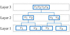
Figure 2. An illustrative example of hierarchical structure.

Typically, we can use a tree to represent a hierarchical structure. In a tree, each parent node can have different numbers of child nodes, which can also be the parents of the nodes in the next layer. Recall the example given by Figure 1, which shows the hierarchical structure of genres of a book. The genre Literature & Fiction is the parent node of several child nodes, such as ${\it GenreFiction}$, Historical Fiction, etc. The child node ${\it HistoricalFiction}$ is also the parent of other nodes such as ${\it Political}$. The leaf nodes are those who have no child such as ${\it Political}$. From this example, it is easily observed that the hierarchical structure can naturally be characterized by the parent-child relation. With this intuition, next we introduce how to incorporate the structure information from parent-child perspective.

The item characteristic matrix ${\bf V}\in\mathbb{R}^{d\times m}$ shows the latent representations of items in a $d$-dimensional latent space. To incorporate the hierarchical structure, we can further decompose ${\bf V}$ into two matrices ${\bf V}^{1}\in\mathbb{R}^{m_{1}\times m}$ and ${\bf V}^{2\prime}\in\mathbb{R}^{d\times m_{1}}$ such that ${\bf V}\approx{\bf V}^{2\prime}{\bf V}^{1}$, assuming there are $m_{1}$ nodes (or sub-categories) in the second layer. Hence, ${\bf V}^{1}$ indicates the parent-child relation between the $m_{1}$ categories in the second layer and $m$ items in the first layer. Moreover, ${\bf V}^{2\prime}$ gives the latent representations of the $m_{1}$ categories. In this way, the latent representation of $v_{j}$ can be expressed by the $j^{th}$ item’s parent categories and their latent representations as ${\bf V}^{2\prime}{\bf V}^{1}(:,j)$. If the structured information has more than two layers, we can further decompose ${\bf V}^{2\prime}$ such that ${\bf V}^{2\prime}\approx{\bf V}^{3\prime}{\bf V}^{2}$, where ${\bf V}^{2}\in\mathbb{R}^{m_{2}\times m_{1}}$ denotes the parent-child relation between categories in the third and second layers, respectively. Similarly, ${\bf V}^{3\prime}\in\mathbb{R}^{d\times m_{3}}$ denotes the representations of $m_{2}$ categories in the third layer. With this, $j^{th}$ item’s representation can be expressed by ${\bf V}^{3\prime}{\bf V}^{2}{\bf V}^{1}(:,j)$.

The above process can be repeated $q$-$1$ times to capture hierarchical structure of $q$ layers as follows:

(6) $${\bf V}\approx{\bf V}^{q}\cdots{\bf V}^{3}{\bf V}^{2}{\bf V}^{1}$$

where ${\bf V}^{i}\in\mathbb{R}^{m_{i}\times m_{i-1}}(1\leq i<q)$, ${\bf V}^{q}\in\mathbb{R}^{d\times m_{q-1}}$ and $m_{0}=m$.

The parent-child relations indicated by Eq. (6) are implicit and they should be in conformity with explicit ones suggested by hierarchical side information. To achieve this, next we extend Eq. (6) to incorporate the structures in the side information. Let ${\bf T}^{k}\in\mathbb{R}^{m_{k-1}\times m_{k}}$ indicate the parent-child relation between categories in layer $k$ and layer $k+1$ of the hierarchical structure of side information. Specifically, ${\bf T}^{k}(i,j)=1$ denotes that the $i^{th}$ category in layer $k$ is the child of $j^{th}$ category in layer $k+1$. Figure 2 gives an example, where ${\bf T}^{2}\in\mathbb{R}^{2\times 1}$ and ${\bf T}^{2}(1,1)=1,{\bf T}^{2}(2,1)=1$. Thus, the hierarchical structure can be defined by the set $\mathcal{T}=\{{\bf T}^{1},{\bf T}^{2},\cdots,{\bf T}^{q}\}$, assuming there are $q$ layers. Intuitively, the presentation of a parent category should be aggregated from those of all the child categories it contains. Thus, a natural way to capture the parent-child relations in $\mathcal{T}$ is to make parent representations denoted as ${\bf V}^{q}\cdots{\bf V}^{i}$ to be close to the aggregation of their children’s representations denoted as ${\bf V}^{q}\cdots{\bf V}^{i-1}$.

In this work, we choose the mean function to be the aggregation function due to its computational efficiency and leave exploring other choices as one future work. Thus, the structure indicated by the item side information can be captured as follows:

$$\min\underbrace{\sum_{i=2}^{q}\|{\bf V}^{q}\cdots{\bf V}^{i}-{\bf V}^{q}\cdots{\bf V}^{i-1}{\bf Q}^{i-1}\|_{F}^{2}}_{f^{v}({\bf V}^{i},{\bf Q}^{i-1})}$$

where ${\bf Q}^{k}$ is the normalized version of ${\bf T}^{k}$ and ${\bf Q}^{k}(i,j)=\frac{{\bf T}^{k}(i,j)}{\sum_{i=1}^{m_{k-1}}{\bf T}^{k}(i,j)}$.

In a similar way, we can also incorporate hierarchical information of users as:

$$\min\underbrace{\sum_{i=2}^{p}\|{\bf U}^{i}\cdots{\bf U}^{p}-{\bf P}^{i-1}{\bf U}^{i-1}\cdots{\bf U}^{p}\|_{F}^{2}}_{f^{u}({\bf U}^{i},{\bf P}^{i-1})}$$

where ${\bf U}^{i}\in\mathbb{R}^{n_{i-1}\times n_{i}}$ and ${\bf P}^{k}(i,j)=\frac{{\bf C}^{k}(i,j)}{\sum_{i=1}^{n_{k-1}}{\bf C}^{k}(i,j)}$ is the normalized version of ${\bf C}^{k}\in\mathbb{R}^{n_{k-1}\times n_{k}}$, which indicates the parent-child relationship in hierarchical side information of users. $p$ is number of layers of the hierarchy and $1\leq i<p$.

2.4. The Proposed Framework HIRE

Previous subsections introduce the model components that aim to capture both flat and hierarchical side information. Combining them, the framework HIRE is to solve the following optimization problem:

(7) $$\min_{\begin{subarray}{c}{\bf U}^{1},\cdots,{\bf U}^{p},{\bf S}^{u},{\bf W}^{u}\\ {\bf V}^{1},\cdots,{\bf V}^{q},{\bf S}^{v},{\bf W}^{v}\end{subarray}} f({\bf U},{\bf V})+\alpha f^{u}({\bf U}^{i},{\bf P}^{i-1})+\beta f^{v}({\bf V}^{i},{\bf Q}^{i-1})$$

$$+\gamma(\|{\bf S}^{u}{\bf U}^{T}-{\bf W}^{u}{\bf X}\|^{2}_{F}+\|{\bar{\bf X}}-{\bf W}^{u}{\tilde{\bf X}}\|_{F}^{2})$$

$$+\theta(\|{\bf S}^{v}{\bf V}-{\bf W}^{v}{\bf Y}\|^{2}_{F}+\|{\bar{\bf Y}}-{\bf W}^{v}{\tilde{\bf Y}}\|_{F}^{2})$$

where ${\bf U}={\bf U}^{1}{\bf U}^{2}\cdots{\bf U}^{p}$ and ${\bf V}={\bf V}^{q}\cdots{\bf V}^{2}{\bf V}^{1}$. $\gamma$ and $\theta$ control the contribution of flat information, $\alpha$ and $\beta$ decides the contribution of hierarchical information. Hence, the proposed framework simultaneously models both flat and hierarchical side information with mathematical coherence. Following the tradition (Koren et al., 2009), we will use the gradient descent method to optimize the formulation of the proposed framework. Next we will use ${\bf U}^{i}$ as one example to illustrate how to get the gradient of parameters due to the page limitation. Before calculating the gradient, we define ${\bf A}^{i}$, ${\bf H}^{i}$, ${\bf D}^{i}$, ${\bf G}_{i}^{k}$ and ${\bf B}_{i}^{k}$ that can be used to simplify the expressions:

$${\bf A}^{i}=\begin{cases}{\bf U}^{1}{\bf U}^{2}\ldots{\bf U}^{i-1},&\mbox{if }i\neq 1\\ {\bf I},&\mbox{if }i=1\end{cases}$$

$${\bf H}^{i}=\begin{cases}{\bf U}^{i+1}\ldots{\bf U}^{p}{\bf V}^{q}\ldots{\bf V}^{1},&\mbox{if }i\neq p\\ {\bf V}^{q}\ldots{\bf V}^{1},&\mbox{if }i=p\end{cases}$$

$${\bf D}^{i}=\begin{cases}{\bf U}^{i+1}{\bf U}^{i+2}\ldots{\bf U}^{p},&\mbox{if }i\neq p\\ {\bf I},&\mbox{if }i=p\end{cases}$$

$${\bf G}_{i}^{k}=\begin{cases}{\bf U}^{k+1}\cdots{\bf U}^{i-1},&\mbox{if }k\neq i-1\\ {\bf I},&\mbox{if }k=i-1\end{cases}$$

$${\bf B}_{i}^{k}={\bf P}^{k}{\bf U}^{k}{\bf G}_{i}^{k}$$

where $1\leq i\leq p$ and $1\leq k<i-1$. By dropping irrelevant terms in Eq. (7), remaining terms related to ${\bf U}^{i}$ are as follows:

$$\mathcal{L}({\bf U}^{i})=\|{\bf M}\odot({\bf R}-{\bf A}^{i}{\bf U}^{i}{\bf H}^{i})\|_{F}^{2}+\lambda\|{\bf U}^{i}\|_{F}^{2}+\alpha\|({\bf I}-{\bf P}^{i}{\bf U}^{i}){\bf D}^{i}\|_{F}^{2}$$

$$+\alpha\sum_{k=1}^{i-1}\|({\bf G}_{i}^{k}-{\bf B}_{i}^{k}){\bf U}^{i}{\bf D}^{i}\|_{F}^{2}+\gamma\|{\bf S}^{u}({\bf A}^{i}{\bf U}^{i}{\bf D}^{i})^{T}-{\bf W}^{u}{\bf X}\|_{F}^{2}$$

Now, we can obtain the gradient of ${\bf U}^{i}$ as:

(8) $$\frac{\partial\mathcal{L}({\bf U}^{i})}{\partial{\bf U}^{i}}={{\bf A}^{i}}^{T}[{\bf M}\odot({\bf A}^{i}{\bf U}^{i}{\bf H}^{i}-{\bf R})]{{\bf H}^{i}}^{T}+\lambda{\bf U}^{i}$$

$$+\alpha\sum_{k=1}^{i-1}({\bf G}_{i}^{k}-{\bf B}_{i}^{k})^{T}({\bf G}_{i}^{k}-{\bf B}_{i}^{k}){\bf U}^{i}{\bf D}^{i}{{\bf D}^{i}}^{T}$$

$$+\alpha{{\bf P}^{i}}^{T}({\bf P}^{i}{\bf U}^{i}{\bf D}^{i}-{\bf D}^{i}){{\bf D}^{i}}^{T}+\gamma{{\bf A}^{i}}^{T}({\bf A}^{i}{\bf U}^{i}{\bf D}^{i}{{\bf S}^{u}}^{T}-{\bf X}^{T}{\bf W}^{u}){\bf S}^{u}{{\bf D}^{i}}^{T}$$

2.4.1. Time Complexity Analysis

The most expensive operations in the optimization process are updating ${\bf U}^{i}$ and ${\bf V}^{i}$, which in each iteration will cost $\mathcal{O}\big{(}nn_{1}n_{i-1}+(2n_{i}n_{i+1}+mm_{1})d+n_{i-1}^{2}(n_{i}+\sum_{k=1}^{i-1}n_{k})\big{)}$ and $\mathcal{O}\big{(}mm_{1}m_{i-1}+(2m_{i}m_{i+1}+nn_{1})d+m_{i-1}^{2}(m_{i}+\sum_{k=1}^{i-1}m_{k})\big{)}$, respectively. Thus, assume $N$ iterations are needed in total, the overall time complexity of the optimization process is $\mathcal{O}\Big{(}\sum_{i}^{p}\big{(}nn_{1}n_{i-1}+(2n_{i}n_{i+1}+mm_{1})d+n_{i-1}^{2}(n_{i}+\sum_{k=1}^{i-1}n_{k})\big{)}+\sum_{i}^{q}\big{(}mm_{1}m_{i-1}+(2m_{i}m_{i+1}+nn_{1})d+m_{i-1}^{2}(m_{i}+\sum_{k=1}^{i-1}m_{k})\big{)}\Big{)}$.

3. Experiments

Table 1. Recommendation performance comparison. All prediction differences between HIRE and other methods are statistically significant.

Methods	MovieLens (100K)			MovieLens (1M)			BookCrossing
	40%	60%	80%	40%	60%	80%	40%	60%	80%
SVD	1.0152	0.9704	0.9491	0.9161	0.9087	0.8947	4.7746	2.8866	2.0899
NMF	1.0352	0.9955	0.9715	0.9446	0.9293	0.9227	2.9381	2.7832	2.6055
I-CF	1.0601	1.0485	1.0343	1.0229	1.0065	0.9975	2.0216	1.9989	2.2250
NeuMF	1.0928	1.0877	1.0849	0.9872	0.9834	0.9825	2.0191	1.8708	1.8586
mSDA-CF	1.0968	1.0891	1.0792	1.0498	1.0482	1.0466	3.0015	2.1992	1.8692
HSR	0.9879	0.9647	0.9376	0.9074	0.8906	0.8742	4.8821	4.1072	3.6137
HIRE	0.9703	0.9398	0.9243	0.8957	0.8778	0.8607	2.3364	1.9193	1.8432

In this section, we firstly introduce the experimental settings. Then, we compare the proposed framework HIRE with representative baselines to answer the first question. Finally, we analyze each model component, which gives answer to the section question. To encourage the reproducible results, we make our code publicly available at: https://github.com/tal-ai/Recommender-Systems-with-Heterogeneous-Side-Information.

3.1. Experimental Settings

We evaluate the proposed framework on three benchmark datasets MovieLens (100K), MovieLens (1M), and BookCrossing and all of them are publicly available (Harper and Konstan, 2016; Ziegler et al., 2005).

• MovieLens (100K) and MovieLens (1M) are collected from a movie review website where users can give movie rating scores on a scale from 1-5. MovieLens (100k) contains 100,000 ratings from 1000 users on 1700 movies and MovieLens (1M) contains 1 million ratings from 6000 users on 4000 movies. For movies, we use genres as hierarchical information; for users, we use age and gender as flat information and occupation as the hierarchical information.

• BookCrossing is a book rating dataset collected from Book-Crossing community and the rating score is from 1 to 10. After basic data cleaning, we get 17028 ratings from 1009 users on 1816 books. For books, we use publish year and author as flat information and publisher as hierarchical information; for users, we use age and location as the flat and hierarchical information, respectively.

For each dataset, we split it into training and test sets such that training set contains $x\%$ of the data and test contains $1-x\%$. We vary $x$ as $\{40,60,80\}$. We choose the commonly used Root Mean Square Error (RMSE) as the measurement metrics of the recommendation performance and lower value of RMSE indicates better performance. In fact, a small improvement in RMSE means a significant improvement of recommender systems (Koren, 2008).

3.2. Recommendation Performance Comparison

In this subsection, we evaluate the recommendation performance of proposed framework by comparing it with following representative baselines:

• SVD (Golub and Reinsch, 1970): It is a matrix factorization technique that factorizes a user-item rating matrix to obtain latent representations of customers and products via singular-value decomposition (SVD). In this method, only rating information is used;

• NMF (Gu et al., 2010): Non-negative matrix factorization (NMF) is one of the most popular algorithms used in recommender systems. Unlike SVD, it adds non-negative constraints to the latent representations. This method also only uses rating information;

• I-CF (Sarwar et al., 2001): This is a item-based collaborative filtering approach that recommends items to users based on the similarity computed from the rating matrix;

• NeuMF (He et al., 2017): NeuMF replaces inner product by combining GMF and MLP neural architectures with sharing embedding layer and is able to significantly improves recommendation performance. In this method, only rating information is used.

• mSDA-CF (Li et al., 2015a): This method integrates matrix factorization and deep feature learning and achieves state-of-the-art performance. It uses both rating and flat side information and ignores hierarchical one.

• HSR (Wang et al., 2018): HSR is a state-of-the-art algorithm which is able to capture both rating and structured side information. However, flat information is ignored in this method.

Note that the parameters of all methods are selected through five-fold cross validation and the details of parameter selection of the proposed framework are discussed in the later subsections. we repeat each experiment five times and report the average performance in Table 1. The following observations can be made from the table:

• NeuMF is likely to outperform other traditional CF methods, which suggests the power of deep learning in recommendations. Currently our basic model is based on matrix factorization and it has great potential to choose NeuMF as the basic model to further improve the performance.

• Systems incorporating side information tend to obtain better performance compared to their corresponding systems without side information. This observation supports the importance of side information.

• The proposed framework HIRE achieves the best performance in most of the cases. We contribute the superior performance to its ability to capture both flat and structured side information. More details regarding the contribution of each component will be discussed in following subsection.

With the above observation, we are able to draw a conclusion to answer the first question: the proposed framework that incorporates heterogeneous side information significantly improves the recommendation performance over the state-of-the-art methods. In the next subsection, we will give a detailed analysis of the contribution from flat and hierarchical side information, respectively.

3.3. Component Analysis

In this subsection, we systematically examine the effect of key components by constructing following model variants:

• HIRE-FU: it eliminates the contribution of flat side information of users by setting $\gamma=0$ in Eq. (7).

• HIRE-FV: it eliminates the contribution of flat side information of items by setting $\theta=0$ in Eq. (7).

• HIRE-SU: it eliminates the contribution of hierarchical side information of users by setting $\alpha=0$ in Eq. (7).

• HIRE-SV: it eliminates the contribution of hierarchical side information of items by setting $\beta=0$ in Eq. (7).

The recommendation performance on MovieLens (100K) is shown in Figure 3. Since we observe similar results on other datasets, we only show that on MovieLens (100K) dataset to save space. From the Figure 3, we can easily observe that HIRE obtains the least RMSE error among all its variants in all cases. This suggests that recommendation performance degrades when ignoring any type of side information. Thus, it is important to incorporate heterogeneous side information in recommender systems.

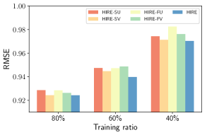
Figure 3. Performance analysis of HIRE with different components.

3.4. Parameter Analysis

In this subsection, we further analyze the sensitivity of the four key parameters $\gamma$, $\theta$, $\alpha$ and $\beta$ that control the contributions of flat side information of users, flat side information of items, hierarchical side information of users, and hierarchical information of items, respectively. In detail, for each of the four parameters, we conduct experiment with the proposed framework by varying the value of it while fixing the others. The performance is shown in Figure 4. Similarly, only performance on MovieLens (100K) is reported due to the space limitation. From both figures, we clearly see that the performance tends to first increase and then decrease, which further supports the importance of side information in recommendations.

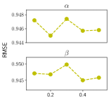
(a) Performance with $\alpha$ abd $\beta$

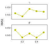
(b) Performance with $\gamma$ and $\theta$

Figure 4. Parameter analysis with $\alpha$, $\beta$, $\gamma$ and $\theta$

4. Related Work

In this section, we give a brief overview of the related recommender systems. A large body of research has been devoted to developing algorithms to improve the performance of recommender systems, which play a crucial role in the increasingly digitalized society. Among them, collaborative filtering based approaches have achieved great success. Roughly, collaborative filtering can be categorized into two type: (1) memory-based approaches (Sarwar et al., 2001; Wang et al., 2006; Melville et al., 2002; Popescul et al., 2001), which aim at exploring neighborhood information of users or items for recommendation; and (2) model-based methods (Koren et al., 2009; Ma et al., 2008; Gu et al., 2010), which try to model the underlying mechanism that governs user rating process. Generally, model-based methods show superior performance than the content-based ones. In particular, Matrix Factorization (MF) based collaborative filtering have gained great popularity due to their high performance and efficiency (Lee and Seung, 1999; Koren et al., 2009; Mnih and Salakhutdinov, 2008; Salakhutdinov and Mnih, 2008; Srebro et al., 2005). Despite of its success, collaborative filtering approaches are known to suffer from data sparsity issues, as the number of items or users is typically very large but the number of ratings is relatively small. One popular way to address this issue is to incorporate the increasingly available side information in the model (Fang and Si, 2011; Vasile et al., 2016; Tang et al., 2016; Adomavicius and Tuzhilin, 2011; Wang et al., 2018; Lu et al., 2012). The majority of studies exploit either only flat side information (Fang and Si, 2011; Adomavicius and Tuzhilin, 2011), or only hierarchical side information (Wang et al., 2018; Lu et al., 2012) due to the challenges brought by the inherent difference between these two types of information. However, our work addresses these challenges and is able to incorporate the two types of information simultaneously.

5. Conclusion

In this paper, we investigate the problem of exploiting heterogeneous side information for recommendations. Specifically, we propose a novel recommendation framework HIRE that is able to capture both flat and hierarchical side information with mathematical coherence. Extensive experiments on three benchmark datasets verify the effectiveness of the framework and demonstrate the impact of both flat and hierarchical side information on recommendation performance.

References

- (1)
- Adomavicius and Tuzhilin (2005) Gediminas Adomavicius and Alexander Tuzhilin. 2005. Toward the next generation of recommender systems: A survey of the state-of-the-art and possible extensions. TKDE 6 (2005), 734–749.
- Adomavicius and Tuzhilin (2011) Gediminas Adomavicius and Alexander Tuzhilin. 2011. Context-aware recommender systems. In Recommender systems handbook. Springer, 217–253.
- Bengio et al. (2013) Yoshua Bengio, Aaron Courville, and Pascal Vincent. 2013. Representation learning: A review and new perspectives. IEEE transactions on pattern analysis and machine intelligence 35, 8 (2013), 1798–1828.
- Chen et al. (2012) Minmin Chen, Zhixiang Xu, Kilian Weinberger, and Fei Sha. 2012. Marginalized denoising autoencoders for domain adaptation. arXiv preprint arXiv:1206.4683 (2012).
- Fang and Si (2011) Yi Fang and Luo Si. 2011. Matrix co-factorization for recommendation with rich side information and implicit feedback. In Proceedings of the 2nd International Workshop on Information Heterogeneity and Fusion in Recommender Systems. ACM, 65–69.
- Golub and Reinsch (1970) Gene H Golub and Christian Reinsch. 1970. Singular value decomposition and least squares solutions. Numerische mathematik 14, 5 (1970), 403–420.
- Gu et al. (2010) Quanquan Gu, Jie Zhou, and Chris Ding. 2010. Collaborative filtering: Weighted nonnegative matrix factorization incorporating user and item graphs. In SDM. SIAM, 199–210.
- Harper and Konstan (2016) F Maxwell Harper and Joseph A Konstan. 2016. The movielens datasets: History and context. Acm transactions on interactive intelligent systems (tiis) 5, 4 (2016), 19.
- He et al. (2017) Xiangnan He, Lizi Liao, Hanwang Zhang, Liqiang Nie, Xia Hu, and Tat-Seng Chua. 2017. Neural collaborative filtering. In WWW. 173–182.
- Koren (2008) Yehuda Koren. 2008. Factorization meets the neighborhood: a multifaceted collaborative filtering model. In KDD. ACM, 426–434.
- Koren et al. (2009) Yehuda Koren, Robert Bell, and Chris Volinsky. 2009. Matrix factorization techniques for recommender systems. Computer 8 (2009), 30–37.
- Lee and Seung (1999) Daniel D Lee and H Sebastian Seung. 1999. Learning the parts of objects by non-negative matrix factorization. Nature 401, 6755 (1999), 788.
- Li et al. (2015b) Jiwei Li, Minh-Thang Luong, and Dan Jurafsky. 2015b. A hierarchical neural autoencoder for paragraphs and documents. arXiv preprint arXiv:1506.01057 (2015).
- Li et al. (2015a) Sheng Li, Jaya Kawale, and Yun Fu. 2015a. Deep collaborative filtering via marginalized denoising auto-encoder. In CIKM. ACM, 811–820.
- Lu et al. (2012) Kai Lu, Guanyuan Zhang, Rui Li, Shuai Zhang, and Bin Wang. 2012. Exploiting and exploring hierarchical structure in music recommendation. In Asia Information Retrieval Symposium. Springer, 211–225.
- Lu et al. (2013) Xugang Lu, Yu Tsao, Shigeki Matsuda, and Chiori Hori. 2013. Speech enhancement based on deep denoising autoencoder.. In Interspeech. 436–440.
- Ma et al. (2008) Hao Ma, Haixuan Yang, Michael R Lyu, and Irwin King. 2008. Sorec: social recommendation using probabilistic matrix factorization. In CIKM. ACM, 931–940.
- Melville et al. (2002) Prem Melville, Raymond J Mooney, and Ramadass Nagarajan. 2002. Content-boosted collaborative filtering for improved recommendations. Aaai/iaai 23 (2002), 187–192.
- Menon et al. (2011) Aditya Krishna Menon, Krishna-Prasad Chitrapura, Sachin Garg, Deepak Agarwal, and Nagaraj Kota. 2011. Response prediction using collaborative filtering with hierarchies and side-information. In Proceedings of the 17th ACM SIGKDD international conference on Knowledge discovery and data mining. ACM, 141–149.
- Mnih and Salakhutdinov (2008) Andriy Mnih and Ruslan R Salakhutdinov. 2008. Probabilistic matrix factorization. In NIPS. 1257–1264.
- Ning and Karypis (2012) Xia Ning and George Karypis. 2012. Sparse linear methods with side information for top-n recommendations. In RecSys. ACM, 155–162.
- Popescul et al. (2001) Alexandrin Popescul, David M Pennock, and Steve Lawrence. 2001. Probabilistic models for unified collaborative and content-based recommendation in sparse-data environments. In UAI. Morgan Kaufmann Publishers Inc., 437–444.
- Ricci et al. (2015) Francesco Ricci, Lior Rokach, and Bracha Shapira. 2015. Recommender systems: introduction and challenges. In Recommender systems handbook. Springer, 1–34.
- Salakhutdinov and Mnih (2008) Ruslan Salakhutdinov and Andriy Mnih. 2008. Bayesian probabilistic matrix factorization using Markov chain Monte Carlo. In ICML. ACM, 880–887.
- Sarwar et al. (2001) Badrul Sarwar, George Karypis, Joseph Konstan, and John Riedl. 2001. Item-based collaborative filtering recommendation algorithms. In WWW. ACM, 285–295.
- Srebro et al. (2005) Nathan Srebro, Jason Rennie, and Tommi S Jaakkola. 2005. Maximum-margin matrix factorization. In NIPS. 1329–1336.
- Su and Khoshgoftaar (2009) Xiaoyuan Su and Taghi M Khoshgoftaar. 2009. A survey of collaborative filtering techniques. Advances in artificial intelligence 2009 (2009).
- Tang et al. (2016) Jiliang Tang, Suhang Wang, Xia Hu, Dawei Yin, Yingzhou Bi, Yi Chang, and Huan Liu. 2016. Recommendation with Social Dimensions.. In AAAI. 251–257.
- Vasile et al. (2016) Flavian Vasile, Elena Smirnova, and Alexis Conneau. 2016. Meta-prod2vec: Product embeddings using side-information for recommendation. In RecSys. ACM, 225–232.
- Wang et al. (2006) Jun Wang, Arjen P De Vries, and Marcel JT Reinders. 2006. Unifying user-based and item-based collaborative filtering approaches by similarity fusion. In SIGIR. ACM, 501–508.
- Wang et al. (2018) Suhang Wang, Jiliang Tang, Yilin Wang, and Huan Liu. 2018. Exploring Hierarchical Structures for Recommender Systems. TKDE 30, 6 (2018), 1022–1035.
- Yang et al. (2016) Jie Yang, Zhu Sun, Alessandro Bozzon, and Jie Zhang. 2016. Learning hierarchical feature influence for recommendation by recursive regularization. In RecSys. ACM, 51–58.
- Zhang et al. (2014) Jie Zhang, Shiguang Shan, Meina Kan, and Xilin Chen. 2014. Coarse-to-fine auto-encoder networks (cfan) for real-time face alignment. In ECCV. Springer, 1–16.
- Ziegler et al. (2005) Cai-Nicolas Ziegler, Sean M McNee, Joseph A Konstan, and Georg Lausen. 2005. Improving recommendation lists through topic diversification. In WWW. ACM, 22–32.