A Sufficient Statistic for Influence
in Structured Multiagent Environments

Abstract

Making decisions in complex environments is a key challenge in artificial intelligence (AI). Situations involving multiple decision makers are particularly complex, leading to computational intractability of principled solution methods. A body of work in AI has tried to mitigate this problem by trying to distill interaction to its essence: how does the policy of one agent influence another agent? If we can find more compact representations of such influence, this can help us deal with the complexity, for instance by searching the space of influences rather than the space of policies. However, so far these notions of influence have been restricted in their applicability to special cases of interaction. In this paper we formalize influence-based abstraction (IBA), which facilitates the elimination of latent state factors without any loss in value, for a very general class of problems described as factored partially observable stochastic games (fPOSGs). On the one hand, this generalizes existing descriptions of influence, and thus can serve as the foundation for improvements in scalability and other insights in decision making in complex multiagent settings. On the other hand, since the presence of other agents can be seen as a generalization of single agent settings, our formulation of IBA also provides a sufficient statistic for decision making under abstraction for a single agent. We also give a detailed discussion of the relations to such previous works, identifying new insights and interpretations of these approaches. In these ways, this paper deepens our understanding of abstraction in a wide range of sequential decision making settings, providing the basis for new approaches and algorithms for a large class of problems.

1 Introduction

One of the important ideas in the development of algorithms for multiagent systems (MASs) is the identification of compressed representations of the information that is relevant for an agent (?, ?, ?, ?, ?, ?, ?, ?, ?, ?, ?, ?, ?). For instance, when a cook and a waiter collaborate, the waiter might not need to know all details of how the cook prepares the food; it may be sufficient if he/she has an understanding of the time that it will take.

In this paper we investigate abstractions that aim at decomposing structured MASs into a set of smaller interacting problems (?, ?). In particular, we describe in detail the concept of influence-based abstraction (IBA), which facilitates the abstraction of latent state variables without sacrificing task performance. It constructs a smaller, local model for one of the agents given the policies of the other agents. IBA consists of two steps: first, we compute a so-called influence point—a more abstract representation of how an agent’s local problem is affected by other agents and external (i.e., non-local) parts of the problem—, second, this influence is used to construct the smaller influence-augmented local model (IALM). This IALM can subsequently be used to compute a best response.

IBA does not only give a new perspective on best-response computations themselves, but this new perspective also has broader implications. For instance, it forms the basis of influence search (?, ?, ?, ?), which can provide significant speedup for multiagent planning by searching the space of joint influences rather than the potentially much bigger space of joint policies. It also can underpin guarantees on the quality of heuristic solutions, by considering optimistic influences (?), or approximate influences (?). While in this article, we assume that the model (which can be seen as a specific type of dynamic Bayesian network) is known in advance, future work could consider learning such representations. Moreover, IBA can serve as inspiration, in the context of deep reinforcement learning, for neural network architectures that compute approximate versions of influence, which can improve learning, both in terms of speed as well as performance (?).

This article gives a formal definition of influence that can be used to perform IBA for general factored partially observable stochastic games (fPOSGs) (?, ?), and proves that an IALM constructed using this definition of influence in fact allows computation of an exact best-response. In other words, it shows that this description of influence is a sufficient statistic of the policy of the other agents: it is sufficient to predict observations and rewards and to thereby optimize value. This article extends our previous paper (?) in the following ways:

1. it provides a complete proof of the claimed exactness of IBA;

2. it elaborates on a number of technical subtleties, such as dealing with multiple sources of influence, and specifying initial beliefs in the IALM;

3. it provides an extension of IBA and corresponding proofs to fPOSGs with intra-stage dependencies, which are critical for the expressiveness of the formalism (cf. Section 4.1.1);

4. it provides additional illustration and explanation, making the concept of IBA more accessible;

5. it deepens the discussion of the relation to special cases of fPOSGs, and more explicitly identifies ways in which future work can improve scalability of these sub-classes;

6. it provides a much more extensive discussion of related work, including the more recent work on deep reinforcement learning (RL). Specifically, by building on the theoretical results provided in this paper, it generates insights into the nature of the ‘approximate value factorization’ assumption which has been successfully exploited by a popular class of deep RL methods.

Additionally, in Section 3 we make a simple (but, in the context of IBA, novel) observation: the presence of other agents can be seen as a generalization of single agent settings, which directly implies that our formulation of IBA also provides a sufficient statistic for decision making under abstraction for a single agent. While there is a multitude of performance loss bounds available for abstractions, e.g., see ? (?, ?, ?, ?, ?, ?, ?), these are usually based on assumed quality bounds on the transition probabilities and rewards of the abstracted model (see Section 8.3 for more details). In contrast, our work here shows how an abstracted model can preserve exact transition and reward predictions, by ‘remembering’ appropriate elements of the local history. In the words of ? (?), we detail an approach to perfectly “uncover […] hidden state” in abstractions for a large class of structured problems.

As such, the contributions of this paper are of a theoretical nature: they provide a principled understanding of lossless abstractions in structured (multiagent) decision problems by providing a formal framework that gives a unified perspective on previous work, while at the same time providing new insights and extending the scope of applicability. The main technical result is the proof of sufficiency given in Section 6: the smaller influence-augmented local model produced by IBA can be used instead of the original larger model without any loss in solution quality (i.e., value). The proof is not only a certification of the theory, it also serves a practical purpose: it isolates the core technical property that needs to hold for sufficiency, thus providing 1) insight into how abstraction of latent state factors affects value, 2) a derivation that can be used to obtain a simplification of influence in simpler cases, and 3) a recipe of how to prove similar results for more complex settings.

This paper is organized as follows: First, Section 2 provides the necessary background by introducing single and multiagent models for decision making. Section 3 introduces the concept of computing best responses (using global value functions) to the policies of other agents and the concept of ‘local form models’ which formalizes a desired abstraction for an agent. Next, in Section 4, we bring these concepts together: we show how an agent can locally compute a best-response (compute a local value function) provided it is given an influence point. Section 5 extends this framework to problems with intra-stage dependencies. Section 6 then presents the main proof of sufficiency of our influence points, i.e., it shows that they provide sufficient information to compute optimal policies without any loss in value. Section 7 discusses reinterpretations of previous work on forms of influence-based abstraction in our more general framework, while Section 8 details the relations to other related work. Finally, Section 9 concludes.

2 Background

Here we concisely provide background on some of the models that we use. The main purpose is to introduce the notation formally. For an extensive introduction to partially observable Markov decision processes (POMDPs) we refer to ? (?) and ? (?), for an introduction to multiagent variants see ? (?, ?) and ? (?).

Unavoidably, this manuscript contains a fair amount of terminology and mathematical notations. To aid the reader we have included a list of acronyms (Appendix B) and a list of recurring notation (Appendix C).

2.1 Single-Agent Models: POMDPs

Partially observable Markov decision processes, or POMDPs, provide a formal framework for the interaction of an agent with a stochastic, partially observable environment. That is, they provide an agent with the capabilities to reason about both action uncertainty as well as state uncertainty.

2.1.1 Model

A POMDP is a discrete time model, in which the agent selects an action at every time step or stage. It extends the regular Markov decision process (MDP) (?) to settings in which the state of the environment cannot be observed. It can be formally defined as follows.

Definition 1 (POMDP).

A partially observable Markov decision process (POMDP) is defined as a tuple $\mathcal{M}^{POMDP}=\left\langle\mathcal{S},{\mathcal{A}},T,R,{\mathcal{O}},O,H,{{{b}}^{0}}\right\rangle$ with the following components:

• $\mathcal{S}$ is a (finite) set of states $s$. The state at some stage $t$ is denoted ${s}^{t}$;

• ${\mathcal{A}}$ is the (finite) set of actions ${a}$;

• $T$ is the transition probability function, that specifies $T(s^{\prime}|s,{a})=\Pr({s}^{t+1}=s^{\prime}\mid{s}^{t}=s,\ {a}^{t}={a}),$ the probability of a next state $s^{\prime}$ given a current state $s$ and action ${a}$. This directly demonstrates the primed shorthand notation we will occasionally use;

• $R$ is the immediate reward function $R:\mathcal{S}\times\mathcal{A}\times\mathcal{S}\rightarrow$. With $R(s,{a},s^{\prime})$ we denote the reward specified for a particular transition $s,a,s^{\prime}$;

• ${\mathcal{O}}$ is the set of observations;

• $O$ is the observation probability function, which specifies $O({o}|{a},s^{\prime})=\Pr({o}^{t+1}={o}\mid{a}^{t}={a},\,{s}^{t+1}=s^{\prime})$, the probability of a particular observation ${o}$ after ${a}$ and resulting state $s^{\prime}$;

• $H$ is the horizon of the problem as mentioned above;

• ${{b}}^{0}\in\Delta(\mathcal{S})$, is the initial state distribution at time $t=0$.

In many cases, the set of states is huge, and states can be thought of as composed of values assigned to different variables:

Definition 2 (Factored POMDP).

In a factored POMDP (fPOMDP), the state space $\mathcal{S}$ is spanned by a set $\mathcal{F}=\left\{{F}^{1},\dots,{F}^{|\mathcal{F}|}\right\}$ of state variables ${F}^{k}$ (that are also called factors). Each of these can take values from its domain ${\mathcal{F}}^{k}$, such that the set of states is defined as $\mathcal{S}={\mathcal{F}}^{1}\times\dots\times{\mathcal{F}}^{|\mathcal{F}|}$.

The merit of such a factored POMDP is that, by making the structure of the problem (i.e., how different factors influence each other) explicit, the model can be much more compact. In particular, the initial state distribution can be compactly represented as a Bayesian network (?, ?, ?), and the transition and reward model can be specified compactly using a two-stage dynamic Bayesian network (2DBN) (?), and a similar approach can be taken for the observation model (?). (An example of a 2DBN will be discussed in Figure 2 2.)

The fPOMDP model is closely related to the framework of influence diagrams (?, ?). In fact, by unrolling (over time) the 2DBN we create an influence diagram. We point out, however, that our notion of influence (i.e., the influence point and the resulting influence-based abstraction we will detail in Section 4) is novel; it has not been considered in influence diagrams.

2.1.2 Beliefs

In contrast to regular MDPs, in a POMDP the agent cannot observe the state; it only observes the observations. However, the observations are not a Markovian signal: i.e., the last observation ${o}^{t}$ made by the agent does not provide the same amount of information (to predict the rewards and the future of the process) as the action-observation history (AOH), the entire history of actions and observations ${\vec{h}}^{t}=\left({a}^{0},{o}^{1},\dots,{a}^{t-1},{o}^{t}\right)$. This means that in general the agent needs to select its actions based on ${\vec{h}}^{t}$ in order to achieve optimal performance.

Luckily, for a POMDP this history can be summarized compactly as a belief, which is defined as the posterior probability distribution over states given the history:

$${{b}}(s)\operatorname{\triangleq}\Pr(s|{{b}}^{0},{\vec{h}}^{t}).$$

The belief does not only summarize the history, it does so in a lossless way. That is, a belief is a sufficient statistic for optimal decision making (?); it allows an agent to reach the same performance as an agent that would act optimally based on the AOH ${\vec{h}}^{t}$.

This belief can be recursively computed, which means that an agent can update its belief as it interacts with its environment. We write ${{b}}^{\prime}=BU({{b}},{a},{o})$, where $BU({{b}},{a},{o})$ is the belief update operator that, given a previous belief $b$ taken action ${a}$ and received observation ${o}$, produces the next belief:

$$\forall s^{\prime}\qquad BU({{b}},{a},{o})(s^{\prime})=\frac{1}{\Pr({o}|{{b}},{a})}\Pr({o}|{a},s^{\prime})\sum_{s}\Pr(s^{\prime}|s,{a}){{b}}(s).$$ (2.1)

Here, $\Pr({o}|{{b}},{a})$ is a normalization constant:

$$\Pr({o}|{{b}},{a})=\mathbf{E}_{{s}\sim{{b}},{s}^{\prime}\sim T({s},{a},\cdot)}\left[O({a},{s}^{\prime},{o})\right]=\sum_{s^{\prime}}\Pr({o}|{a},s^{\prime})\sum_{s}\Pr(s^{\prime}|s,{a}){{b}}(s).$$

2.1.3 Policies and Value Functions

In a POMDP, the agent employs a policy, ${\pi}$, to interact with its environment. Such a policy is a (deterministic) mapping from beliefs to actions. Note that, given the initial belief ${{b}}^{0}$, such a policy will specify an action for each observation history.

The goal of the decision maker, or agent, in the POMDP is to choose a policy ${\pi}$ that maximizes the expected (discounted) cumulative reward:

$$\mathbf{E}\left[\sum_{t=0}^{H-1}\gamma^{t}R({s}^{t},{a}^{t},{s}^{t+1})|{{b}}^{0},{\pi}\right],$$ (2.2)

here

• $H$ is the horizon, i.e., the number of time steps, or stages, for which we want to plan,

• the expectation is over sequences of states and observations induced by the policy ${\pi}$,

• $\gamma\in[0,1]$ is the discount factor.

In this work, we focus on the finite-horizon case, in which it is typical (but not necessary) to assume $\gamma=1$.

For a finite-horizon POMDP, the optimal (action-)value function for stage $t$ can be expressed as

$${Q}^{t}({{b}},{a})=\begin{cases}R({{b}},{a}),&t=H-1\\ R({{b}},{a})+\gamma\sum_{{o}}\Pr({o}|{{b}},{a})V^{{t+1}}(BU({{b}},{a},{o})),&\text{otherwise}\end{cases}$$ (2.3)

where $V^{{t+1}}({{b}}^{\prime})=\max_{{a}^{\prime}}{Q}^{t+1}({{b}}^{\prime},{a}^{\prime})$ is the value of acting optimally in the next time step and $R({{b}},{a})$ is the expected immediate reward:

$$R({{b}},{a})=\mathbf{E}_{s\sim{{b}},s^{\prime}\sim T(\cdot|s,{a})}\left[R(s,{a},s^{\prime})\right]=\sum_{s}{{b}}(s)\sum_{s^{\prime}}\Pr(s^{\prime}|s,{a})R(s,{a},s^{\prime}).$$ (2.4)

2.2 Multiagent Models: POSGs

The POMDP model can be extended to include multiple self-interested agents as follows.

Definition 3 (POSG).

A partially observable stochastic game (POSG) is defined as a tuple $\mathcal{M}^{POSG}=\left\langle\mathcal{D},\mathcal{S},\mathcal{A},T,\mathcal{R},\mathcal{O},O,H,{{{b}}^{0}}\right\rangle$ with the following components:

• $\mathcal{D}=\{{1},\dots,{n}\}$ is the set of $n$ agents.

• $\mathcal{S}$ is a (finite) set of states.

• $\mathcal{A}={\mathcal{A}}_{1}\times\dots\mathcal{A}_{n}$ is the set of joint actions $a=\left\langle{a}_{1},\dots,{a}_{n}\right\rangle$, with ${\mathcal{A}}_{i}$ the set of individual actions for agent $i$.

• $T$ is the transition probability function, that now depends on joint actions: $T({s}^{t+1}|{s}^{t},{a}^{t})=\Pr({s}^{t+1}|{s}^{t},{a}^{t})$.

• $\mathcal{R}=\left\langle{R}_{1},\dots R_{n}\right\rangle$ is the collection of immediate reward functions (one for each agent). Each ${R}_{i}:\mathcal{S}\times\mathcal{A}\times\mathcal{S}\rightarrow$ maps from states, joint actions and next states to an immediate reward for agent $i$.

• $\mathcal{O}={\mathcal{O}}_{1}\times\dots\times{\mathcal{O}}_{n}$ is the set of joint observations $o=\langle{o}_{1},\dots,{o}_{n}\rangle$, with ${\mathcal{O}}_{i}$ the set of individual observations for agent $i$,

• $O$ is the observation probability function, which specifies $\Pr(o|a,s^{\prime})$, the probability of a particular joint observation $o$ after $a$ and resulting state $s^{\prime}$.

• $H$ is the horizon of the problem as mentioned above.

• ${{b}}^{0}\in\Delta(\mathcal{S})$, is the initial state distribution at time $t=0$.

Since in a POSG each agent has its own goal, there no longer is a definition of optimality. Instead it is customary to focus on game-theoretic solution concepts (?). Such solutions, e.g., Nash equilibria, typically specify a tuple of policies $\pi=\left\langle{\pi}_{1},\dots,{\pi}_{n}\right\rangle$, one for each agent, that are in equilibrium. In general, we will refer to a tuple of policies $\pi$ as a joint policy.

Of course, it is also possible to consider cooperative teams of agents. In this case, we align the goals of the agents by giving them the same reward function:

Definition 4 (Dec-POMDP).

A decentralized partially observable Markov decision process (Dec-POMDP) is a POSG where all agents share the same reward function: $\forall_{i,j}\;{R}_{i}={R}_{j}$.

Since interests are aligned, in a Dec-POMDP we can speak about optimality. Moreover, there is guaranteed to be at least one deterministic joint policy that is optimal (?). As was the case for POMDPs, we can also consider variants of the multiagent models with factored state spaces. We will refer to these as factored POSGs (fPOSGs) and factored Dec-POMDPs (fDec-POMDPs) (?).

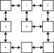
Figure 1: A possible instantiation of the House Search problem: 1, 2 represent the starting locations of the agents, while ‘T’ encodes the possible locations of the target.

As an example, we consider the House Search problem (?), in which a team of robots must find a target (say a remote control) in a house with multiple rooms. This task is representative of an important class of problems in which a team of agents needs to locate objects or targets. In House Search the assumption is that a prior probability distribution over the location of the target is available and that the target is stationary or moves in a manner that does not depend on the strategy used by the searching agents.

Example.

The House Search environment can be represented by a graph, as illustrated in Figure 1 for the case of two agents. At every time step each agent can stay in the current room or move to a next one. The location of an agent $i$ at time step $t$ is denoted $l_{i}^{t}$ and that of the target is denoted $l_{tgt}^{t}$. In general, the target could move with probabilities $p(l_{tgt}^{{}^{\prime}}|l_{tgt})$. The actions (movements) of each agent have a specific cost $c_{i}(l_{i},{a}_{i})$ (e.g., the energy consumed by navigating to a next room) and can fail; we allow for stochastic transitions $p(l_{i}^{\prime}|l_{i},{a}_{i})$. Also, each robot might receive a penalty $c_{time}$ for every time step that the target is not found yet. When a robot is in (or near) the same node as the target, there is a probability of detecting the target $p(detect_{i}|l_{tgt},l_{i})$, which will be modeled by a Boolean state variable ‘target found’ ${f}^{t}$, which both agents can observe (thus modeling a communication channel which the agents can only use to inform each other of detection). When the target is detected, the agents also receive a reward $r_{detect}$. Given the prior distribution and model of target behavior, the goal is to optimize the sum (over time) of rewards, thus trading off movement cost and probability of detecting the target as soon as possible. In this paper, we focus on the local perspective of a protagonist agent and therefore will assume that each agent has its individual rewards (so the POSG setting).

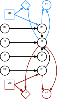
(a) With intra-stage connections.

(b) Without intra-stage connections.

Figure 2: Factored representation of the House Search problem. Actions, observations and rewards of the first agent are in light blue, while those of agent 2 are in dark red. State variables are in black. We use standard shapes for influence diagrams: rectangles for actions, circles for random variables, and diamonds for rewards  (e.g., ?) .

Figure 2a demonstrates how a two-stage dynamic Bayesian network (2DBN) can be used to compactly represent the transition, observation, and reward model (?). For instance, for each state variable at a state $t+1$, the 2DBN shows which other entities (state factors and actions) influence it. The figure illustrates that most dependencies are across-stage (e.g., $l_{2}^{t}$ influences $l_{2}^{t+1}$) but that it is also possible to have intra-stage dependencies (ISDs). For instance, whether the target will be detected at stage $t+1$ depends on $l_{2}^{t+1}$ not on $l_{2}^{t}$. The representation of the transition model is compact since it can be represented as a product of conditional probability tables (CPTs), each of which are exponential only in the number of incoming dependencies. So as long as the number of incoming connections is limited, the transition probabilities can be represented compactly. Figure 2a also shows that this type of representation can also be employed for observation probabilities, as well as rewards.

Since ISDs complicate the notation and definition of influence, we also consider a version of the problem that has no intra-stage connections, shown in Figure 2b. For rewards and observations, intra-stage connections are still allowed. (In fact, since the observation probabilities in the standard POMDP definition depend on the next state $s^{\prime}$, there is no way of representing them without intra-stage connections). Note that this is a slightly different problem than the problem represented in Figure 2a: in the problem without ISDs the agents have a chance of detecting the target at stage $t+1$ if they are co-located with the target at stage $t$, which means that there is a one-step delay incurred before they receive the reward. This illustrates the fact the ISDs do allow for a more expressive model, and that therefore developing theory that support such connections is an important goal.

To facilitate easier exposition, in Section 4 we will first introduce the concept of influence-based abstraction without ISDs. These will be considered in Section 5. Before we can jump to the topic of influence-based abstraction, however, we will need to discuss decision problems from a local perspective, in Section 3, which covers problems with ISDs.

3 Best Responses and Local-Form Models

In contrast to the typical solutions to POSGs and Dec-POMDPs, which try and identify a joint policy as the solution, this paper focuses on the local perspective of an individual agent. From this perspective, the agent’s goal is to compute a best-response to the policies used by other agents. That is, given a multiagent model with state uncertainty (either a POSG or Dec-POMDP) and given some policy for the other agents ${\pi}_{-{i}}=\left\langle{\pi}_{1},\dots,{\pi}_{i-1},{\pi}_{i+1},\dots,{\pi}_{n}\right\rangle$, we want to compute the best response ${\pi}_{i}^{BR}$ for agent $i$. Such best-response computation is obviously important for self-interested agents (i.e., in POSGs), but is also an important component in many Dec-POMDP solution methods (?, ?, ?, ?, ?). Also, let us point out that we make no restrictions on the policies employed by the other agents: they are general mappings from the action-observation histories ${\vec{h}}_{j}^{t}$ to probability distributions over actions. For instance, their policies could be learning algorithms such as Q-learning. As such, the setting we consider is very general.

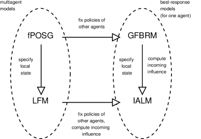
Figure 3: Overview of various models used.

As illustrated in Figure 3, we will consider a number of different types of models in this paper. The starting point is given by the fPOSG or a special case thereof (e.g., a Dec-POMDP). We refer those models as global-form models. For such models, it is possible to directly compute a best-response by fixing the policies of the other agents. We refer to the resulting POMDP as a global-form best-response model (GFBRM); these models will be introduced next. Subsequently, we will introduce local-form models (LFMs), which restrict the state factors that each agent primarily cares about. That is, an agent in an LFM only reasons about a subset of factors. This will then form the basis for computing best-responses in such a local model, called influence-augmented local model (IALM), which will be enabled by influence-based abstraction introduced in Section 4.

3.1 Global-Form Best-Response Model

In this section we define a Global-Form Best-Response Model (GFBRM) that an agent can use in order to compute a best-response in a general POSG. We first define this model and then talk about value functions for this model.

Specification of the Model

The basic idea of defining a best-response model is shown in Figure 4. By fixing ${\pi}_{-{i}}$, the policies of the other agents, all the choice nodes are turned into random variables that now depend on the AOHs that those agents observed (?). So the key construct here is that the AOH of the other agent(s) is made part of the hidden state (often termed latent state factors) of the best-response model. This can be formalized as follows.

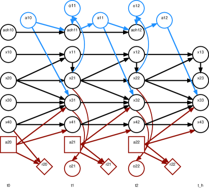
Figure 4: A hypothetical global-form best-response model for agent 2, unrolled over time. This model has a number of state factors ${F}^{k}$. In addition, the action-observation history ${\vec{h}}_{1}^{t}$ (or, more general, internal state) of agent 1 can be interpreted as a state factor in this model.

Definition 5 (Global-Form Best-Response Model).

Let $\mathcal{M}^{POSG}=\left\langle\mathcal{D},\mathcal{S},\mathcal{A},T,\mathcal{R},\mathcal{O},O,H,{{{b}}^{0}}\right\rangle$ be a (f)POSG and let ${\pi}_{-{i}}$ be a profile of policies for all agents but $i$. We say that the POMDP $\mathcal{M}_{i}^{GFBR}(\mathcal{M}^{POSG},{\pi}_{-{i}})=\left\langle\bar{{\mathcal{S}}_{i}},{\mathcal{A}}_{i},\bar{T}_{i},\bar{R}_{i},{\mathcal{O}}_{i},\bar{O}_{i},H,\bar{{{b}}_{i}}{}^{0}\right\rangle$ is a Global-Form Best-Response Model (GFBRM) for agent $i$, where

• $\bar{{\mathcal{S}}_{i}}$ is the set of augmented states ${\bar{s}}_{i}^{t}=\langle s,{\vec{h}}_{-{i}}^{t}\rangle$ that specify an underlying state of the POSG as well as an AOH history for all the other agents.

• ${\mathcal{A}}_{i},{\mathcal{O}}_{i}$ are the (unmodified) sets of actions and observations for agent $i$.

• The transitions

  $$\bar{T}_{i}({\bar{s}}_{i}^{t+1}|{\bar{s}}_{i}^{t},{a}_{i}^{t}) = \bar{T}_{i}(\langle{s}^{t+1},{\vec{h}}_{-{i}}^{t+1}\rangle|\langle{s}^{t},{\vec{h}}_{-{i}}^{t}\rangle,{a}_{i}^{t})$$ (3.1)

  $$= \bar{T}_{i}(\langle{s}^{t+1},\left({\vec{h}}_{-{i}}^{t},{a}_{-{i}}^{t},{o}_{-{i}}^{t+1}\right)\rangle|\langle{s}^{t},{\vec{h}}_{-{i}}^{t}\rangle,{a}_{i}^{t})$$

  $$= \Pr({o}_{-{i}}^{t+1},{s}^{t+1},{a}_{-{i}}^{t}|{s}^{t},{a}_{i}^{t},{\vec{h}}_{-{i}}^{t})$$

  $$= \Pr({o}_{-{i}}^{t+1}|{a}_{i}^{t},{a}_{-{i}}^{t},{s}^{t+1})\Pr({s}^{t+1}|{s}^{t},{a}_{i}^{t},{a}_{-{i}}^{t})\Pr({a}_{-{i}}^{t}|{\vec{h}}_{-{i}}^{t})$$

  $$= \left[\sum_{{o}_{i}^{t+1}}O({o}^{t+1}|{a}^{t},{s}^{t+1})\right]T({s}^{t+1}|{s}^{t},{a}^{t}){\pi}_{-{i}}({a}_{-{i}}^{t}|{\vec{h}}_{-{i}}^{t})$$

  with ${\pi}_{-{i}}({a}_{-{i}}^{t}|{\vec{h}}_{-{i}}^{t})=\prod_{j\neq i}{\pi}_{j}({a}_{j}^{t}|{\vec{h}}_{j}^{t})$ the probability of ${a}_{-{i}}^{t}$ given ${\vec{h}}_{-{i}}^{t}$ according to ${\pi}_{-{i}}$.

• The observations

  $$\bar{O}_{i}({o}_{i}^{t+1}|{a}_{i}^{t},{\bar{s}}_{i}^{t+1}) = \bar{O}_{i}({o}_{i}^{t+1}|{a}_{i}^{t},\langle{s}^{t+1},\left({\vec{h}}_{-{i}}^{t},{a}_{-{i}}^{t},{o}_{-{i}}^{t+1}\right)\rangle)$$ (3.2)

  $$= \Pr({o}_{i}^{t+1}|{a}_{i}^{t},{a}_{-{i}}^{t},{s}^{t+1},{o}_{-{i}}^{t+1})$$

  $$= \frac{\Pr({o}_{i}^{t+1},{o}_{-{i}}^{t+1}|{a}_{i}^{t},{a}_{-{i}}^{t},{s}^{t+1})}{\Pr({o}_{-{i}}^{t+1}|{a}_{i}^{t},{a}_{-{i}}^{t},{s}^{t+1})}$$

  $$= \frac{O({o}^{t+1}|{a}^{t},{s}^{t+1})}{\sum_{{o}_{i}^{t+1}}O({o}^{t+1}|{a}^{t},{s}^{t+1})}$$

  (Note that ${o}^{t+1}=\left\langle{o}_{i}^{t+1},{o}_{-{i}}^{t+1}\right\rangle$, such that the summation is over the component of ${o}^{t+1}$ corresponding to agent $i$).

• $\bar{R}_{i}$ is the augmented reward model

  $$\bar{R}_{i}({\bar{s}}_{i}^{t},{a}_{i}^{t},{\bar{s}}_{i}^{t+1}) = \bar{R}_{i}(\langle{s}^{t},{\vec{h}}_{-{i}}^{t}\rangle,{a}_{i}^{t},\langle{s}^{t+1},{\vec{h}}_{-{i}}^{t+1}=\left({\vec{h}}_{-{i}}^{t},{a}_{-{i}}^{t},{o}_{-{i}}^{t+1}\right)\rangle)$$ (3.3)

  $$= {R}_{i}({s}^{t},{a}_{i}^{t},{a}_{-{i}}^{t},{s}^{t+1})$$

  Note that ${a}_{-{i}}^{t}$ is specified by ${\bar{s}}_{i}^{t+1}$.

• $H$ is the (unmodified) horizon.

• $\bar{{{b}}_{i}}{}^{0}$ is the initial belief.

A GFBRM is a POMDP, which means that an agent can track a belief, which is now a distribution over augmented states ${\bar{s}}_{i}=\langle{s}^{t},{\vec{h}}_{-{i}}^{t}\rangle$, as usual. We will refer to such beliefs as global-form beliefs, denoted ${b}_{i}^{g}$. The initial global-form belief follows directly from the initial belief of the POSG. Since at the first stage, the history of the other agents is the empty history $()$, it is trivially constructed from ${{b}}^{0}$:

$$\forall_{s}\ {b}_{i}^{g,{0}}(\left\langle s,()\right\rangle)\operatorname{\triangleq}{{b}}^{0}(s).$$

Note that the description of the GFBRM depends rather crucially on the fact that we choose AOHs for the representation of the internal state of the other agent(s). That is, we assume that the policies of the other agent(s) are based on their AOHs. While this is a very general model, other models of other agents with a more limited description of internal state (e.g., finite state controllers) can be useful too. For such more compact descriptions, however, it is not always possible to construct a POMDP model with an independent transition and observation model. Instead, one may need to replace $\bar{T},\bar{O}$ by a combined ‘dynamics function’ $\bar{D}$ that specifies $\bar{D}({\bar{s}}_{i}^{t+1},{o}_{i}^{t+1}|{\bar{s}}_{i}^{t},{a}_{i}^{t})$. For more details see ? (?).

Value Function

Since a GFBRM is just a POMDP, all POMDP theory and solution methods apply. E.g., the optimal (action-)value function is given by:

$${Q}_{i}^{t}({b}_{i}^{g},{a}_{i}^{t})={R}_{i}({b}_{i}^{g},{a}_{i}^{t})+\gamma\sum_{{o}_{i}^{t+1}}\Pr({o}_{i}^{t+1}|{b}_{i}^{g},{a}_{i}^{t}){V}_{i}^{t+1}(BU({b}_{i}^{g},{a}_{i}^{t},{o}_{i}^{t+1}))$$ (3.4)

where

$${R}_{i}({b}_{i}^{g},{a}_{i}^{t}) =\mathbf{E}_{{\bar{s}}_{i}^{t}\sim{b}_{i}^{g},{\bar{s}}_{i}^{t+1}\sim\bar{T}_{i}({\bar{s}}_{i}^{t},{a}_{i}^{t},\cdot)}\left[\bar{{R}_{i}}({\bar{s}}_{i}^{t},{a}_{i}^{t},{\bar{s}}_{i}^{t+1})\right]$$

$$=\sum_{{s}^{t}}\sum_{{s}^{t+1}}\sum_{{a}_{-{i}}}\Pr({s}^{t+1}|{s}^{t},a){R}_{i}({s}^{t},a,{s}^{t+1})\sum_{{\vec{h}}_{-{i}}^{t}}\Pr({a}_{-{i}}|{\vec{h}}_{-{i}}^{t}){b}_{i}^{g}({s}^{t},{\vec{h}}_{-{i}}^{t})$$ (3.5)

(see Appendix A.1.1) and

$$\Pr({o}_{i}^{t+1}|{b}_{i}^{g},{a}_{i}^{t})=\mathbf{E}_{{\bar{s}}_{i}^{t}\sim{b}_{i}^{g},{\bar{s}}_{i}^{t+1}\sim\bar{T}_{i}({\bar{s}}_{i}^{t},{a}_{i}^{t},\cdot)}\left[\bar{O}_{i}({o}_{i}^{t+1}|{a}_{i}^{t},{\bar{s}}_{i}^{t+1})\right]\\ =\sum_{{s}^{t}}\sum_{{s}^{t+1}}\sum_{{a}_{-{i}}}\sum_{{o}_{-{i}}^{t+1}}\Pr({s}^{t+1}|{s}^{t},a)\Pr({o}^{t+1}|a,{s}^{t+1})\sum_{{\vec{h}}_{-{i}}^{t}}\Pr({a}_{-{i}}|{\vec{h}}_{-{i}}^{t},{\pi}_{-{i}}){b}_{i}^{g}({s}^{t},{\vec{h}}_{-{i}}^{t})$$ (3.6)

(see Appendix A.1.2.)

Solution of the GFBRM gives the best-response value for agent $i$:

$${V}_{i}({\pi}_{-{i}})\operatorname{\triangleq}{V}_{i}^{0}({b}_{i}^{g,{0}}).$$ (3.7)

3.2 Local-Form Model

GFBRMs allow an agent $i$ to compute a best-response policy against the fixed policies ${\pi}_{-{i}}$ of the other agents. A difficulty here is that agent $i$ needs to reason about many state factors as well as the internal state (the action-observation history) of the other agents. That is, drawing an analogy to human interactions, it is like in a simple collaborative task (e.g., carrying a table), we would need to reason over the inner working of our collaborator’s brain, as well as over the sequence of images that he or she perceives. Clearly, such an approach is infeasible in general. To make a step in the direction to overcome this problem, here we introduce local-form models (LFMs) which restrict the set of state factors that each agent primarily cares about, and eliminates the dependence on the AOH of other agents.

Local States

An LFM augments an fPOSG with a function that provides a description of each agent’s local state, i.e., the set of variables that each agent will model as part of its local problem. Local state descriptions comprise potentially overlapping subsets of state factors that will allow us to decompose an agent’s best-response computation from the global state. We start with some definitions.

Definition 6 (Local state function).

The local state function $S:\mathcal{D}\rightarrow 2^{\mathcal{F}}$ maps from agents to subsets of state factors $S({i})\subseteq\mathcal{F}$.

The local state function defines the local state space of each agent. In particular, we say that a state factor $F\in\mathcal{F}$ is modeled by an agent $i$ if it is part of its local state space: $F\in S({i})$.

Definition 7 (Local state space).

The local state space of agent $i$ is defined as the Cartesian product of the values that its modeled state factors can take:

$${\mathcal{X}}_{i}\;\operatorname{\triangleq}\;\prod_{\begin{subarray}{c}k\text{ s.t.}{F}^{k}\in S({i})\end{subarray}}{\mathcal{F}}^{k}$$ (3.8)

(remember that $\mathcal{F}$ is the set of state factors, while ${\mathcal{F}}^{k}$ is the set of values that the $k$-th state factor ${F}^{k}$ can take).

Definition 8 (Observation-relevant factor).

We say that a state factor $F$ is observation-relevant for an agent $i$, denoted $\text{ORel}{}_{i}(F)$, if it affects the probability of the agent’s observation. That is, when in the 2DBN there is a link from ${F}^{t}$ to ${o}_{i}^{t}$ (i.e., $F$ is a parent of ${o}_{i}^{t}$).

Definition 9 (Reward-relevant factor).

Similarly, a state factor $F$ is reward-relevant for an agent $i$, $\text{RRel}{}_{i}(F)$ if it affects the agent’s rewards, i.e., if ${F}^{t}$ or ${F}^{t+1}$ is a parent of ${R}_{i}^{t}$.

We can now define the local-form model.

Definition 10 (Local-form model).

A local-form POSG, also referred to as local-form model (LFM), is a pair $\mathcal{M}^{LFM}=\left\langle\mathcal{M},S\right\rangle$, where $\mathcal{M}$ is an fPOSG and $S$ is a local state function such that, for all agents:

1. All observation-relevant factors are in the local state: $\forall_{{i}}\forall_{F}\;\text{ORel}{}_{i}(F)\implies F\in S({i}).$

2. All reward-relevant factors are in the local state: $\forall_{{i}}\forall_{F}\;\text{RRel}{}_{i}(F)\implies F\in S({i}).$

Modeled and Non-modeled Factors

The basic idea behind the definition of the local-form model is to avoid reasoning over the subset of variables from the global-form model that are superfluous when it comes to computing the best response. Therefore, these non-modeled factors can be abstracted away. The requirements on observation- and reward-relevant factors make certain that the observation probabilities and rewards are still specified in this abstracted model. Note also that this means that we will only be able to abstract away (latent) state variables, not observation variables themselves. We will show that such latent factor abstraction can, in principle, be performed without loss in value. This certainly would not be the case for abstracting away observation variables: in general this would lead to a loss of information and a corresponding drop in achievable value (?).

The focus in this text is on the best-response perspective for one agent $i$. This allows us to divide the set of state factors in ones modeled by agent $i$’s local problem (indicated with $x$) and ones that are not modeled (indicated with $y$). To reduce the notational load, we will no longer distinguish between a factor (${F}^{k}$ above) and its values (${\mathcal{F}}^{k}$ above). In particular, we will simply write

• ${x}^{k}$ (an instantiation of) a modeled factor (with index $k$),

• ${x}_{i}$ (an instantiation of) all modeled factors of agent $i$,

• ${y}^{k}$ (an instantiation of) a non-modeled factor (with index $k$),

• ${y}_{i}$ (an instantiation of) all non-modeled factors of agent $i$,

such that ${s}^{t}=\langle{x}_{i}^{t},{y}_{i}^{t}\rangle$. We stress that ‘modeled’ is different from ‘observed’. In particular, our aim is to construct a smaller POMDP with fewer (modeled) factors, but those factors may not be observable. In fact, all state factors ${x}^{k}$ (and of course also ${y}^{k}$) are expressed as latent variables. When an agent can somehow (noisily) perceive information about ${x}^{k}$, this should be modeled by the observation function: there should be an arrow from such factors to the observation ${o}_{i}$ of the agent and the CPT of ${o}_{i}$ should appropriately express the observability of factor. Note that by construction of the LFM (cf. Definition 10), no such dependencies may exist from a ${y}^{k}$ to ${o}_{i}$. In general, the observation ${o}_{i}$ may itself consists of multiple observation factors, but we will not consider this in this paper.

Transition Probabilities

In an LFM, the probability of the next local state is the marginal of the entire state:

$$\Pr({x}_{i}^{t+1}|{s}^{t},{a}_{i},{a}_{-{i}})=\sum_{{y}_{i}^{t+1}}\Pr({x}_{i}^{t+1},{y}_{i}^{t+1}|{s}^{t},{a}_{i},{a}_{-{i}})$$ (3.9)

In an LFM, just as in a normal fPOSG, the flat transition probabilities on the right hand side of this equation are given by the product of the CPTs. However, from the perspective of an agent $i$ we can now group these CPTs in three different categories: 1) those corresponding to modeled factors that are only affected by other factors and actions that are modeled, 2) those corresponding to modeled factors that are affected by at least one factor or action of the external problem, and 3) those corresponding to non-modeled factors. We will refer to the state factors corresponding to these as:

1. Only-locally-affected factors (OLAFs) ${\mathring{x}}^{k}$. These can have incoming arrows from all modeled factors ${x}_{i}^{t}$ at the previous stage, and from all modeled factors ${x}_{i}^{t+1}$ intra-stage (but, obviously, excluding ${\mathring{x}}^{k,t+1}$ itself, and respecting a non-cyclic structure as any 2DBN).

2. Non-locally-affected factors (NLAFs) ${\tilde{x}}^{k}$. These are affected by at least one non-modeled (intra-stage or previous-stage) factor or action of another agent.

3. Non-modeled factors (NMFs) ${y}^{k}$.

(Note that the oversets on ${x}$ were chosen to resemble ‘o’ and ‘n’ for OLAF and NLAF respectively). These three types of factors are illustrated in Figure 5a, which shows a hypothetical local-form model. Using the introduced notation, we can write the transition probabilities as:

$$\Pr({s}^{t+1}|{s}^{t},{a}_{i},{a}_{-{i}})=\left[\Pr({\mathring{x}}_{i}^{t+1}|\dots)\Pr({\tilde{x}}_{i}^{t+1}|\dots)\Pr({y}_{i}^{t+1}|\dots)\right]\\ =\Pr({\mathring{x}}_{i}^{t+1}|{x}_{i}^{t},{\tilde{x}}_{i}^{t+1},{a}_{i})\Pr({\tilde{x}}_{i}^{t+1}|{x}_{i}^{t},{\mathring{x}}_{i}^{t+1},{y}_{i}^{t},{y}_{i}^{t+1},{a}_{i},{a}_{-{i}})\Pr({y}_{i}^{t+1}|{x}_{i}^{t},{x}_{i}^{t+1},{y}_{i}^{t},{a}_{i},{a}_{-{i}})$$ (3.10)

with

• $\Pr({\mathring{x}}_{i}^{t+1}|{x}_{i}^{t},{\tilde{x}}_{i}^{t+1},{a}_{i})$ representing a product of CPTs of OLAFs ${\mathring{x}}^{k}$:

  $$\Pr({\mathring{x}}_{i}^{t+1}|{x}_{i}^{t},{\tilde{x}}_{i}^{t+1},{a}_{i})=\prod_{k\in OLAF(i)}\Pr({\mathring{x}}^{k,t+1}|{x}_{i}^{t},{x}_{i}^{t+1},{a}_{i})$$ (3.11)

  Note that although such individual factors ${\mathring{x}}^{k,t+1}$ can have intra-stage dependencies on other OLAFs ${\mathring{x}}^{l,t+1}$ (i.e., ${\mathring{x}}^{k,t+1}$ can depend on ${x}_{i}^{t+1}$ which can include other OLAFs ${\mathring{x}}^{l,t+1}$), the product term $\Pr({\mathring{x}}_{i}^{t+1}|{x}_{i}^{t},{\tilde{x}}_{i}^{t+1},{a}_{i})$ itself can only have intra-stage dependencies on ${\tilde{x}}_{i}^{t+1}$.

• $\Pr({\tilde{x}}_{i}^{t+1}|{x}_{i}^{t},{\mathring{x}}_{i}^{t+1},{y}_{i}^{t},{y}_{i}^{t+1},{a}_{i},{a}_{-{i}})$ the product of NLAF probabilities:

  $$\Pr({\tilde{x}}_{i}^{t+1}|{x}_{i}^{t},{\mathring{x}}_{i}^{t+1},{y}_{i}^{t},{y}_{i}^{t+1},{a}_{i},{a}_{-{i}})=\prod_{k\in NLAF(i)}\Pr({\tilde{x}}^{k,t+1}|{x}_{i}^{t},{x}_{i}^{t+1},{y}_{i}^{t},{y}_{i}^{t+1},{a}_{i},{a}_{-{i}})$$ (3.12)

• $\Pr({y}_{i}^{t+1}|{x}_{i}^{t},{x}_{i}^{t+1},{y}_{i}^{t},{a}_{i},{a}_{-{i}})$ the product of probabilities of the NMFs ${y}^{k}$:

  $$\Pr({y}_{i}^{t+1}|{x}_{i}^{t},{x}_{i}^{t+1},{y}_{i}^{t},{a}_{i},{a}_{-{i}})=\prod_{k\in NMF(i)}\Pr({y}^{k,t+1}|{x}_{i}^{t},{x}_{i}^{t+1},{y}_{i}^{t},{y}_{i}^{t+1},{a}_{i},{a}_{-{i}})$$ (3.13)

(a) Illustration of an abstract local-form model for agent 2. Factors can be divided into non-modeled factors (${F}^{1}$), non-locally-affected factors (${F}^{2}$, ${F}^{3}$, shaded in this figure), and locally-affected factors (${F}^{4}$). Also note that ${F}^{4}$ is reward-relevant, while ${F}^{2}$ and ${F}^{3}$ are observation-relevant factors.

(b) Local-form model for agent 2 in the house search problem without intra-stage dependencies. The ‘found’ variable $f$ is the only NLAF since it is affected by NMF ${l}_{1}^{t}.$

Figure 5: Local-form models.

Value Function

An LFM contains an fPOSG and as such best-response values for an agent $i$ can be defined using the techniques discussed above in Section 3.1. In particular, we can just ignore the local state function and apply the definition of Q-value (3.4) with the previously stated definitions of $R_{i}({b}_{i}^{g},{a}_{i})$ (3.5) and $\Pr({o}_{i}^{t+1}|{b}_{i}^{g},{a}_{i})$ (3.6).

Clearly, however, we would like to now rewrite the value function in a way that represents the local structure imposed by the LFM requirements and exploits this for computational benefits. The former is possible: for an LFM, we can indeed derive a expression for $R_{i}({b}_{i}^{g},{a}_{i})$ that is more local (see Appendix A.2.1).

$$R_{i}({b}_{i}^{g},{a}_{i}^{t})=\sum_{{x}_{i}^{t}}\sum_{{x}_{i}^{t+1}}R_{i}({x}_{i}^{t},{a}_{i}^{t},{x}_{i}^{t+1})\Pr({x}_{i}^{t},{x}_{i}^{t+1}|{b}_{i}^{g},{a}_{i}^{t},{\pi}_{-{i}}),$$ (3.14)

where (remember ${s}^{t}=\langle{x}_{i}^{t},{y}_{i}^{t}\rangle$)

$$\Pr({x}_{i}^{t},{x}_{i}^{t+1}|{b}_{i}^{g},{a}_{i}^{t},{\pi}_{-{i}})\operatorname{\triangleq}\sum_{{y}_{i}^{t}}\sum_{{a}_{-{i}}^{t}}\Pr({x}_{i}^{t+1}|{s}^{t},{a}_{i}^{t},{a}_{-{i}}^{t})\sum_{{\vec{h}}_{-{i}}^{t}}\Pr({a}_{-{i}}^{t}|{\vec{h}}_{-{i}}^{t},{\pi}_{-{i}}){b}_{i}^{g}({s}^{t},{\vec{h}}_{-{i}}^{t}).$$ (3.15)

And, similarly, we can find a new, local, expression for the observation probability (Appendix A.2.2):

$$\Pr({o}_{i}^{t+1}|{b}_{i}^{g},{a}_{i}^{t})=\sum_{{x}_{i}^{t+1}}\Pr({o}_{i}^{t+1}|{a}_{i}^{t},{x}_{i}^{t+1})\Pr({x}_{i}^{t+1}|{b}_{i}^{g},{a}_{i}^{t},{\pi}_{-{i}})$$ (3.16)

where

$$\Pr({x}_{i}^{t+1}|{b}_{i}^{g},{a}_{i}^{t})\operatorname{\triangleq}\sum_{{s}^{t}}\sum_{{a}_{-{i}}^{t}}\Pr({x}_{i}^{t+1}|{s}^{t},{a}_{i}^{t},{a}_{-{i}}^{t})\sum_{{\vec{h}}_{-{i}}^{t}}\Pr({a}_{-{i}}^{t}|{\vec{h}}_{-{i}}^{t}{\pi}_{-{i}}){b}_{i}^{g}({s}^{t},{\vec{h}}_{-{i}}^{t}).$$ (3.17)

These new definitions of $R_{i}({b}_{i}^{g},{a}_{i}),\,\Pr({o}_{i}^{t+1}|{b}_{i}^{g},{a}_{i})$ can be used directly in conjunction with the definition of Q-value (3.4).

However, even though these definitions (3.14) and (3.16) are local, they still depend on the global-form belief and this must perform summations over full states ${s}^{t}$ and histories of other agents ${\vec{h}}_{-{i}}^{t}$ via (3.15) and (3.17), rendering them intractable for larger problems. In the next section, we will investigate formulations that are based on more local beliefs to try and overcome this computational hurdle. Before jumping to this, we first state an observation:

Observation.

The presented definition of an LFM with multiple agents is a strict generalization of a single agent problem.

While this is a simple observation, the upshot of this is that the theory of influence-based abstraction that we will introduce in the remainder of this paper also directly applies to single-agent settings. Specifically, the formulas and results we will derive have more specific forms for the single-agent case. We discuss relations to abstraction methods for single-agent settings in Section 8.3.

4 Influence-Based Abstraction

In the previous section we introduced the GFBRM, which could be used to compute a best response against a fixed policy of other agents. This model gives a straightforward way of formulating the problem of computing a best-response. However, it is specified over the global state and internal state of other agents (i.e., their AOHs), which means that solving this model is computationally intractable.

To provide a more localized perspective, the local-form POSG defines for each agent a subset of factors that it should be concerned with. However, even if the policies of the other agents are fixed, it is not clear how an agent $i$ can restrict its reasoning to its local state ${x}_{i}$: the non-modeled factors will still affect the local state transitions. Intuitively, we need to capture the influence that the non-modeled part of the problem exerts on the modeled part.

In this section, we formalize this intuition. In particular, we treat an LFM from the perspective of one agent and consider how that agent is affected by the other agents and can compute a best response against that ‘incoming’ influence.

In an attempt to avoid notation overload, we first present a formulation without considering intra-stage connections. The general formulation that can deal with such connections is given in Section 5.

4.1 Definition of Influence

As discussed in Section 3.1, when the other agents are following a fixed policy, they can be regarded as part of the environment. The resulting decision problem can be represented by the complete unrolled DBN, as we saw in Figure 44. In this figure, a node ${F}^{t}$ is a different node than ${F}^{t+1}$ and an edge at (emerging from) stage $t$ is a different from the edge at $t+1$ that corresponds to the same edge in the 2DBN. Given this uniqueness of nodes and edges, we can define the ‘influence’ as follows.

4.1.1 Influence Links, Sources and Destinations

Intuitively, the influence of other agents is the effect of those edges leading into the agent’s local problem. We say that every directed edge from outside the local model (e.g., from an NMF or action of another agent) to inside the local model (e.g., to a modeled state factor, observation variable, or reward), is an influence link $\langle{u}^{t},{v}^{t}\rangle$, where ${u}^{t}$ is called the influence source and ${v}^{t}$ is the influence destination. In this section, we will assume that influence links traverse a stage of the process (i.e., that the influence source for a destination ${v}^{t}$ lies in the stage $t-1$), but since we will also consider intra-stage influence links at a later point in this document, to keep notation consistent, we label an entire influence link with the stage-index of its destination.

For example, let us consider the House Search problem’s LFM shown in Figure 5b on page 5b. It shows that the link from ${l}_{1}^{t}$, the location of agent 1, to the ‘target found’ variable ${f}^{t+1}$ is an influence link, such that we would write the link as $\left\langle{u}^{t+1}={l}_{1}^{t},{v}^{t+1}={f}^{t+1}\right\rangle$, similarly $\left\langle{u}^{t}={l}_{1}^{t-1},{v}^{t}={f}^{t}\right\rangle$ would denote the influence link in the preceding time step.

Assuming no intra-stage influence links, an influence source ${u}^{t}$ can be either an action ${a}_{j}^{t-1}$ or non-modeled state factor ${y}^{t-1}$. We write ${u}_{\rightarrow i}^{t}=\langle{y}_{u}^{t-1},{a}_{u}^{t-1}\rangle$ for an instantiation of all influence sources exerting influence on agent $i$ at stage $t$. That is, in the case of multiple influence links pointing to modeled factors in stage $t$, ${y}_{u}^{t-1}$ denotes the (value of) influence sources that are state factors, while ${a}_{u}^{t-1}$ corresponds to those influence sources that are actions. For instance, in our House Search example, ${y}_{u}^{t-1}=\{{l}_{1}^{t-1}\},$ while ${a}_{u}^{t-1}=\emptyset$ since there are no actions that are influence sources. We write $\vec{h}{}_{u}^{t-1}$ for the AOHs of those other agents whose action is an influence source (i.e., $\vec{h}{}_{u}^{t-1}$ and ${a}_{u}^{t-1}$ involve the same agents) .

In general, an influence destination can be either a (per definition non-locally-affected) modeled factor ${\tilde{x}}^{t}$, an observation variable ${o}_{i}^{t}$, or a local reward node ${R}_{i}^{t}$. But Definition (10) requires reward- or observation-relevant factors to be included in the local state; effectively we restrict ourselves to the setting where the influence destination is an NLAF. This restriction is without loss in generality: because we will introduce (in Section 5) the machinery to deal with intra-stage influence links, influences on observations and rewards can easily be dealt with by introducing a ‘dummy’ NLAF that acts as a proxy for the observation or reward. A similar construction can be used to deal with settings where actions of other agents would directly influence the observations or rewards of the agent under concern. As such, the capability of dealing with such intra-stage dependencies is critical for the applicability of the theory of influence-based abstraction.

4.1.2 Sufficient Information to Predict Influences: D-Separating Sets

If agent $i$ would in advance know the value of its influence sources at different time steps, it could easily compute its best response by making use of only this knowledge and its local model. For instance, if in the House Search example of Figure 5b5b, we would in advance perfectly know the location of agent 1 at each timestep and thus know the sequence of values for ${l}_{1}^{t}$, we could decouple the local problem by just looking at the appropriate slices of the CPT of ${f}^{t}$.

Of course, this is in general not possible, since the influence sources are random variables. However, the influence exerted on agent $i$ can be captured if we know the probability distribution over their values. That is, in order to predict the probability of some ${\tilde{x}}_{i}^{t+1}$ (i.e., an influence destination) agent $i$ only cares about the following marginal probability

$$\sum_{{u}_{\rightarrow i}^{t+1}}\Pr({\tilde{x}}_{i}^{t+1}|{x}_{i}^{t},{a}_{i}^{t},{u}_{\rightarrow i}^{t+1})\Pr({u}_{\rightarrow i}^{t+1}|\ldots),$$ (4.1)

where the dots ($\ldots$) indicate any information that agent $i$ needs to predict the probability of the values of the influence sources as accurately as possible. Moreover, since these probabilities will be used to plan a best response, correlations between influence sources and local states are important. This unfortunately means that in general, we might need to condition $\Pr({u}_{\rightarrow i}^{t+1}|...)$ on the entire history of actions, observations and and local states.

Fortunately, it turns out that in many cases we can find substantially more compact representations of the conditional probability of ${u}_{\rightarrow i}^{t+1}$, by making use of the concept of d-separation in graphical models (?, ?). In particular, when two nodes $A,B$ in a Bayesian network are d-separated given some of subsets ${D}$ of evidence nodes, then $A$ and $B$ are conditionally independent given ${D}$, which means that $\Pr(A|D,B)=\Pr(A|D)$ and vice versa. Whether nodes are d-separated can be easily checked, by applying a small set of rules on the graph (?, chapter 8).

Now, we can define the influence as a conditional probability distribution over ${u}_{\rightarrow i}^{t+1}$, given a d-separating set. Specifically, let ${D}_{i}^{t+1}$ be a subset of variables (possibly including state factors and actions) in the local problem of agent $i$ at stages $0,\dots,t$,

Definition 11 (D-separating set).

${D}_{i}^{t+1}$ is a d-separating set for agent $i$’s influence at stage $t+1$ if and only if it d-separates ${y}_{u}^{t},\vec{h}{}_{u}^{t}$ from ${x}_{i}^{t},{\vec{h}}_{i}^{t}$. That is, if:

$$\forall_{{y}_{u}^{t},{\vec{h}}_{u}^{t}}\qquad\Pr({y}_{u}^{t},{\vec{h}}_{u}^{t}|{x}_{i}^{t},{\vec{h}}_{i}^{t},{D}_{i}^{t+1},{{b}}^{0},{\pi}_{-{i}})=\Pr({y}_{u}^{t},{\vec{h}}_{u}^{t}|{D}_{i}^{t+1},{{b}}^{0},{\pi}_{-{i}}).$$ (4.2)

This definition implies that remembering more than ${D}_{i}^{t+1}$ is not useful for predicting ${y}_{u}^{t},{\vec{h}}_{u}^{t}$ and hence for predicting ${u}_{\rightarrow i}^{t+1}=\langle{y}_{u}^{t},{a}_{u}^{t}\rangle$. Given their policies, the actions of other agents only depend on their AOHs. We note that when the other agents use simpler (e.g., memoryless) policies, one might not need to predict the full action observation history for agents whose actions are influence sources. Instead we will only need to predict relevant part, denoted $\rho({\vec{h}}_{u}^{t})$. Similarly, there might be a sufficient statistic $\sigma$ that summarizes ${D}_{i}^{t+1}$ and still is enough to provide the conditional independence. In such case we would only need

$$\forall_{{y}_{u}^{t},{\vec{h}}_{u}^{t}}\qquad\Pr({y}_{u}^{t},\rho({\vec{h}}_{u}^{t})|{x}_{i}^{t},{\vec{h}}_{i}^{t},\sigma({D}_{i}^{t+1}),{{b}}^{0},{\pi}_{-{i}})=\Pr({y}_{u}^{t},\rho({\vec{h}}_{u}^{t})|\sigma({D}_{i}^{t+1}),{{b}}^{0},{\pi}_{-{i}}).$$ (4.3)

To avoid a further burden on notation, we will not explicitly consider these special cases, and in our description assume that we condition on the values of the variables in the d-separating set. However, we will see examples of such more compact description of the information needed to predict the influence sources.

Deciding on ${D}_{i}^{t+1}$ needs to be done in advance to compute the influence. When the d-separating set is compressed, $\sigma({D}_{i}^{t+1}),$ this will typically involve input by the human designer. However, we note that efficient algorithms are known to compute a minimal d-separating set (?, ?, ?) in cases where this would be infeasible to do by hand.

Example.

Figure 6 illustrates a d-separating set ${D}_{i}^{3}$ for agent $i=2$ in House Search. It shows that, in order to accurately compute the probability of influence source ${l}_{1}^{2}$, agent 2 needs to condition on ${f}^{0:2}$, the history of the found variable, as well as the histories of the location of the target $l_{tgt}$ and its own location ${l}_{2}$. This dependence on the history in general leads to large conditioning sets, but in many cases the history can be represented more compactly. For instance, in House Search the ‘found’ variable can only switch on (not off) which means that its history ${f}^{0:t}$ can be summarized compactly. In cases where the target is static the same holds for ${l}_{tgt}^{0:t}$.

Figure 6: Illustration of the incoming influence on protagonist agent $i=2$ in House Search at stage $t=3$. ${f}^{3}$ is the only influence destination, with influence source ${y}_{u}^{2}={l}_{1}^{2}$ (i.e., ${u}_{\rightarrow i}^{3}=\left\langle{l}_{1}^{2}\right\rangle$). The shaded nodes indicate the d-separating set ${D}_{i}^{3}$, which, in accordance with (4.2), d-separates the influence source ${l}_{1}^{2}$, from agent 2’s AOH ${\vec{h}}_{i}^{t}$ and possibly remaining other local variables ${x}_{i}^{t}$ (in this case there are no such variables, but one could imagine adding a battery life variable for agent 2).

Example.

Figure 7 describes a variant of the planetary exploration domain (?). Here agent 2 is a mars rover which is tasked with navigating to some goal. Agent 1 is a satellite which can aid the rover by planning a path, but this will use up computational resources and battery power modeled by ${bt}_{1}^{t}$ (which it may want to use to support other rovers too, for instance). In the figure this is illustrated by the fact that the action of agent 1 ${a}_{1}\in\{NOOP,PLAN\}$ (which now is the influence source) determines if there is a plan available for agent 2, modeled by a binary variable $pl$ (which is the influence destination). In this example, the d-separating set only contains this variable $pl$. Again its history can be compactly summarized: as having the plan can only turn true, we can just store the time (if any) at which $pl$ was switched to true.

Figure 7: Illustration of the influence experienced by the mars rover (agent $i=2$) at stage $t=3$ in the planetary exploration domain. If the satellite (agent 1) computes and transmits a plan (pl), the rover can more effectively navigate from that point onward.

4.1.3 The Influence Exerted on Agent $i$

Given the above machinery, we can now state our definition of influence:

Definition 12 (Incoming Influence).

The incoming influence at stage $t+1$, denoted ${I}_{\rightarrow i}^{t+1}({\pi}_{-{i}})$, is a conditional probability distribution over values of the influence sources ${u}_{\rightarrow i}^{t+1}$:

$$I({u}_{\rightarrow i}^{t+1}|{D}_{i}^{t+1})\operatorname{\triangleq}\sum_{\vec{h}{}_{u}^{t}}\Pr({a}_{u}^{t}|\vec{h}{}_{u}^{t})\Pr({y}_{u}^{t},\vec{h}{}_{u}^{t}|{D}_{i}^{t+1},{{b}}^{0},{\pi}_{-{i}}).$$ (4.4)

In order to predict ${a}_{u}^{t}$ (the ‘influence source actions’) we need to predict the action-observation histories of the corresponding agents $\vec{h}{}_{u}^{t}$, but otherwise these histories are not needed and can thus be marginalized out. Note that, to reduce notational burden we drop arguments that can be inferred, such as ${{b}}^{0},{\pi}_{-{i}}$. That is, $I({u}_{\rightarrow i}^{t+1}|{D}_{i}^{t+1})$ is shorthand for ${I}_{\rightarrow i}^{t+1}({u}_{\rightarrow i}^{t+1}|{D}_{i}^{t+1},{{b}}^{0},{\pi}_{-{i}})$. In cases where we want to refer to this distribution as a whole, we will write ${I}_{\rightarrow i}^{t+1}({\pi}_{-{i}})$, or use the shorthand ${I}_{\rightarrow i}^{t+1}$.

We will also say that this is the influence exerted on agent $i$ at stage $t$ or experienced by agent $i$ at stage $t+1$. So far, these notions coincide, but when we consider intra-stage connections in the next section, we will discriminate between these concepts.

Finally, we are in position to specify the complete influence on agent $i$:

Definition 13 (incoming influence point).

An incoming influence point ${I}_{\rightarrow i}({\pi}_{-{i}})$ for agent $i$, specifies the incoming influences for all stages ${I}_{\rightarrow i}({\pi}_{-{i}})=\left({I}_{\rightarrow i}^{1}({\pi}_{-{i}}),\dots,{I}_{\rightarrow i}^{H}({\pi}_{-{i}})\right)$.

As we will see in the remainder of this paper, an influence point contains all the information about the non-modeled part of the problem that agent $i$ needs to compute a best response ‘locally’, i.e., only using its local model and that influence point. This can bring computational benefits for instance when there would be changes in the local model that require repeatedly performing planning, or in cases where the influence point can be computed easily. This form of influence-based abstraction, however, is not providing a free lunch (?): in general computing the incoming influences (4.4) for the different stages comprise a set of challenging inference problems. Fortunately, traction can still be gained in many special cases of problems identified in past work (?, ?, ?, ?, ?, ?, ?, ?, ?, ?, ?), and IBA gives a unified perspective on these. Moreover, it can be used as tool to identify further special cases that allow for efficient solution, such as the class of ND-POMDPs discussed in Section 7. Given the potential benefits of using influence representations (?), such future search for special cases of problems that allow for compact influence specifications together with the inference algorithms that efficiently compute these is an important line of research. Our definition of influence in this section provides the general framework in which these special cases should be sought.

4.2 The Influence-Augmented Local Model (IALM)

Given the above definition of influence, we can now define a smaller local model for our protagonist agent $i$. The main idea is that given an incoming influence point, agent $i$ no longer needs to reason over the non-modeled part of the problem. Instead, it can use the influence to compute marginal probabilities as expressed by (4.1), and this will allow it to compute an exact best-response.

In this section, we will first investigate a single NLAF and how the influence on it can be incorporated. Then we move to talk about the case where multiple variables in the local state $S({i})$ are non-locally affected. Then we proceed to the formal definition of the IALM, and how it can be solved.

4.2.1 Induced CPTs

In the case of a single influence destination, we can interpret (4.1) as constructing a new ‘influence-induced’ CPT:

Definition 14 (Induced CPT).

Let ${\tilde{x}}^{t+1}$ be an influence destination, and ${u}^{t+1}$ (the instantiation of) the corresponding influence sources. Given the influence ${I}_{\rightarrow i}^{t+1}({\pi}_{-{i}})$, and its d-separating set ${D}_{i}^{t+1}$, we define the induced CPT for ${\tilde{x}}^{t+1}$ as the CPT that has probabilities:

$$p_{{I}_{\rightarrow i}^{t+1}}({\tilde{x}}^{t+1}|{x}_{i}^{t},{D}_{i}^{t+1},{a}_{i})=\sum_{{u}_{\rightarrow i}^{t+1}=\left\langle{y}_{u}^{t},{a}_{u}\right\rangle}\Pr({\tilde{x}}^{t+1}|{x}_{i}^{t},{a}_{i},{u}_{\rightarrow i}^{t+1})I({u}_{\rightarrow i}^{t+1}|{D}_{i}^{t+1})$$ (4.5)

It is important to note that an induced CPT is specified purely in local terms, i.e., making use of variables that are modeled by our protagonist agent $i$. Therefore, the basic idea is that we can now define a smaller local model—which we will call the Influence-Augmented Local Model (IALM)—by replacing the CPTs of influence destinations (i.e., NLAFs) by induced CPTs.

4.2.2 Dealing With Multiple NLAFs

In case that there are multiple NLAFs, i.e., multiple variables ${\tilde{x}}^{t+1}$ in the local state space $S({i})$ that are affected non-locally at the same stage $t+1$, the story is slightly more involved, since we need to deal with their correlations.

Ideally, we would want to treat induced CPTs in the same way as normal CPTs; that is, we would represent the joint probability of NLAFs as a the product of induced CPTs:

$$\Pr({\tilde{x}}_{i}^{t+1}|{x}_{i}^{t},{D}_{i}^{t+1},{a}_{i},{I}_{\rightarrow i}^{t+1})=\prod_{k\in NLAF(i)}p_{{I}_{\rightarrow i}^{t+1}}({\tilde{x}}^{k,t+1}|{x}_{i}^{t},{D}_{i}^{t+1},{a}_{i}).$$ (4.6)

However, in general this is not possible since the different ${\tilde{x}}^{k,t+1}$ are correlated via any common influence sources. That is, in general the probability is given by:

$$\Pr({\tilde{x}}_{i}^{t+1}|{x}_{i}^{t},{D}_{i}^{t+1},{a}_{i},{I}_{\rightarrow i}^{t+1})=\sum_{{u}_{\rightarrow i}^{t+1}=\left\langle{y}_{u}^{t},{a}_{u}\right\rangle}I({u}_{\rightarrow i}^{t+1}|{D}_{i}^{t+1})\prod_{k\in NLAF(i)}\Pr({\tilde{x}}^{k,t+1}|{x}_{i}^{t},{a}_{i},{u}_{\rightarrow i}^{t+1})$$ (4.7)

Of course, in certain cases a factorization as induced CPTs is possible. The above equations directly make clear when this is the case.

Proposition 1.

If each NLAF ${\tilde{x}}^{k,t+1}$ has its own influence sources ${u}^{k,t+1}$ (and these do not overlap), and if these sources are conditionally independent given ${D}_{i}^{t+1}$:

$$I({u}_{\rightarrow i}^{t+1}|{D}_{i}^{t+1})=\prod_{k\in NLAF(i)}I({u}^{k,t+1}|{D}_{i}^{t+1}),$$

then the joint probability of NLAFs factorizes as the product of induced CPTs as shown in (4.6).

Proof.

Under stated conditions, we can rewrite as follows:

$$\eqref{eq:P(NLAFS)__general}= \sum_{{u}_{\rightarrow i}^{t+1}=\left\langle\dots,{u}^{k,t+1},\dots\right\rangle}I({u}_{\rightarrow i}^{t+1}|{D}_{i}^{t+1})\prod_{k\in NLAF(i)}\Pr({\tilde{x}}^{k,t+1}|{x}_{i}^{t},{a}_{i},{u}^{k,t+1})$$

$$= \sum_{{u}_{\rightarrow i}^{t+1}=\left\langle\dots,{u}^{k,t+1},\dots\right\rangle}\left[\prod_{k\in NLAF(i)}I({u}^{k,t+1}|{D}_{i}^{t+1})\right]\prod_{k\in NLAF(i)}\Pr({\tilde{x}}^{k,t+1}|{x}_{i}^{t},{a}_{i},{u}^{k,t+1})$$

$$= \sum_{{u}_{\rightarrow i}^{t+1}=\left\langle\dots,{u}^{k,t+1},\dots\right\rangle}\prod_{k\in NLAF(i)}I({u}^{k,t+1}|{D}_{i}^{t+1})\Pr({\tilde{x}}^{k,t+1}|{x}_{i}^{t},{a}_{i},{u}^{k,t+1})$$

$$= \prod_{k\in NLAF(i)}\sum_{{u}^{k,t+1}}I({u}^{k,t+1}|{D}_{i}^{t+1})\Pr({\tilde{x}}^{k,t+1}|{x}_{i}^{t},{a}_{i},{u}^{k,t+1})=\eqref{eq:P(NLAFS)__product-of-ICPTS}\qed$$

4.2.3 The IALM: A Formal Model to Incorporate Influence

Here we formally define the IALM, which is a non-stationary POMDP, since at every stage the influence destinations can be influenced in a different manner.

Definition 15 (IALM).

Given an LFM, $\mathcal{M}^{LFM}$, and profile of policies for other agents ${\pi}_{-{i}}$, an Influence-Augmented Local Model (IALM) for agent $i$ is a POMDP $\mathcal{M}_{i}^{IALM}(\mathcal{M}^{LFM},{\pi}_{-{i}})=\left\langle\bar{\mathcal{S}},{\mathcal{A}}_{i},\bar{T}_{i},\bar{R}_{i},{\mathcal{O}}_{i},\bar{O}_{i},H,{b}_{i}^{l,{0}}\right\rangle$, where

• $\bar{\mathcal{S}}$ is the set of augmented states ${\bar{s}}_{i}^{t}=\langle{x}_{i}^{t},{D}_{i}^{t+1}\rangle$ that specify an underlying local state of the POSG, as well as the d-separating set ${D}_{i}^{t+1}$ for the next-stage influences. Note that ${D}_{i}^{t+1}$ typically needs to include certain state factors for stage $t$, such that ${x}_{i}^{t}$ and ${D}_{i}^{t+1}$ both will specify such variables. This is no problem, as long as they specify consistent assignments; we define $\bar{\mathcal{S}}$ to be the set of states that are consistent.

• ${\mathcal{A}}_{i},{\mathcal{O}}_{i}$ are the (unmodified) sets of actions and observations for agent $i$.

• The transition function $\bar{T}_{i}({\bar{s}}_{i}^{t+1}|{\bar{s}}_{i}^{t},{a}_{i}^{t})$ which we will discuss in detail shortly.

• The observation function $\bar{O}_{i}({o}_{i}^{t+1}|{a}_{i}^{t},{\bar{s}}_{i}^{t+1})=O({o}_{i}^{t+1}|{a}_{i}^{t},{x}_{i}^{t+1})$, since agent $i$’s observations only depend on its local state (cf. Definition 10, property 1).

• The reward function $\bar{{R}_{i}}({\bar{s}}_{i}^{t},{a}_{i}^{t},{\bar{s}}_{i}^{t+1})={R}_{i}({x}_{i}^{t},{a}_{i}^{t},{x}_{i}^{t+1})$, since agent $i$’s rewards only depend on its local state (cf. Definition 10, property 2).

• $H$ is the unmodified horizon.

• ${b}_{i}^{l,{0}}$ is the initial state distribution, which is a local-form belief. It is a distribution over augmented states ${\bar{s}}_{i}^{0}=\langle{x}_{i}^{0},{D}_{i}^{1}\rangle$. Since for the first stage ${D}_{i}^{1}$ can only contain elements from ${x}_{i}^{0}$, it can trivially be constructed from a probability distribution over ${x}_{i}^{0}$, and such a distribution can be constructed from ${{b}}^{0}$, as we discuss in a bit more detail below.

In defining $\bar{T}_{i}$ and ${b}_{i}^{l,{0}}$, a few subtleties arise that we now discuss.

Transition Probabilities

Clearly, the IALM’s transition probabilities should express

$$\bar{T}_{i}({\bar{s}}_{i}^{t+1}|{\bar{s}}_{i}^{t},{a}_{i}^{t})\operatorname{\triangleq}\Pr(\langle{x}_{i}^{t+1},{D}_{i}^{t+2}\rangle|\langle{x}_{i}^{t},{D}_{i}^{t+1}\rangle,{a}_{i}^{t},{I}_{\rightarrow i}^{t+1}).$$ (4.8)

For such probabilities to be specified, we need some further requirements on the d-separating sets. In particular, we require that (the instantiation of) ${D}_{i}^{t+2}$ is fully specified by ${x}_{i}^{t},{a}_{i}^{t},{x}_{i}^{t+1}$ and ${D}_{i}^{t+1}$.

Definition 16 (d-set update function).

The d-set update function is a function $d$ that takes the previous-stage d-separating set and the latest transition, and that returns the next d-separating set:

$${D}_{i}^{t+2}=d({x}_{i}^{t},{a}_{i}^{t},{x}_{i}^{t+1},{D}_{i}^{t+1}).$$

In other words: $d$ ‘selects’ the variables from ${x}_{i}^{t},{a}_{i}^{t},{x}_{i}^{t+1},{D}_{i}^{t+1}$ such that it forms the next d-separating set.

Given a d-set update function we can write:

$$\Pr(\langle{x}_{i}^{t+1},{D}_{i}^{t+2}\rangle|\langle{x}_{i}^{t},{D}_{i}^{t+1}\rangle,{a}_{i}^{t},{I}_{\rightarrow i}^{t+1})=\Pr({x}_{i}^{t+1}|\langle{x}_{i}^{t},{D}_{i}^{t+1}\rangle,{a}_{i}^{t},{I}_{\rightarrow i}^{t+1})\boldsymbol{1}_{\{{D}_{i}^{t+2},d({x}_{i}^{t},{a}_{i}^{t},{x}_{i}^{t+1},{D}_{i}^{t+1})\}},$$

where $\boldsymbol{1}_{\{\cdot,\cdot\}}$ denotes the Kronecker delta function.

A typical way to fulfill the requirement that ${D}_{i}^{t+2}$ is fully specified by ${x}_{i}^{t},{a}_{i}^{t},{x}_{i}^{t+1}$ and ${D}_{i}^{t+1}$ is to assume that the d-separating sets for all stages are chosen as the history of the same subset ${D}_{i}\subseteq S(i)$ of modeled features.

Example.

Looking at Figure 6 on page 6, the d-separating set ${D}_{2}^{3}$ for predicting ${f}^{3}$ is given by the history of the ‘found’, ‘location of target’ and ‘location of agent 2’ variables. So we can write ${D}_{2}=\left\{f,{l}_{tgt},{l}_{2}\right\}$, and define ${D}_{2}^{3}$ to be its history at stage $t=2$: ${D}_{2}^{3}=\vec{D}{}_{2}^{2}$.

The probabilities $\Pr({x}_{i}^{t+1}|\langle{x}_{i}^{t},{D}_{i}^{t+1}\rangle,{a}_{i}^{t})$ are now factored as the product of the CPTs of the OLAFs and the induced probabilities for the NLAFs:

$$\bar{T}_{i}({\bar{s}}_{i}^{t+1}|{\bar{s}}_{i}^{t},{a}_{i}^{t})\operatorname{\triangleq}\Pr({x}_{i}^{t+1}|\langle{x}_{i}^{t},{D}_{i}^{t+1}\rangle,{a}_{i}^{t},{I}_{\rightarrow i}^{t+1})\boldsymbol{1}_{\{{D}_{i}^{t+2},d({x}_{i}^{t},{a}_{i}^{t},{x}_{i}^{t+1},{D}_{i}^{t+1})\}},\\ =\Pr({\tilde{x}}_{i}^{t+1}|\langle{x}_{i}^{t},{D}_{i}^{t+1}\rangle,{a}_{i}^{t},{I}_{\rightarrow i}^{t+1})\Pr({\mathring{x}}_{i}^{t+1}|{x}_{i}^{t},{\tilde{x}}_{i}^{t+1},{a}_{i})\boldsymbol{1}_{\{{D}_{i}^{t+2},d({x}_{i}^{t},{a}_{i}^{t},{x}_{i}^{t+1},{D}_{i}^{t+1})\}}.$$ (4.9)

Here the first term is given by (4.7) and the second term is given by (3.11).

Initial Local State Distribution

(a) The Bayesian network $G^{0}$ representing the initial belief.

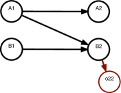
(b) The 2DBN (a conditional Bayesian network) $G^{\rightarrow}$ representing the transition and observation probabilities.

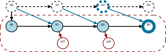
(c) The unrolled network $G=\text{unroll}(G^{0},G^{\rightarrow})$. To convert it to an IALM, the local-form initial belief ${b}_{i}^{l,{0}}(B^{0})$ and incoming influences ${I}_{\rightarrow i}^{t+1}(A^{t}|B^{0},\dots,B^{t})$ need to be computed via inference. See text for further explanation.

Figure 8: Construction of the IALM.

Here we discuss some of the issues involved in defining the initial belief in the IALM. Note that in a factored models such as fPOSGs, the initial state distribution ${{b}}^{0}$ is specified as a Bayesian network $G^{0}$. Together with the 2DBN, $G^{\rightarrow}$ (which in fact is a conditional probability distribution), it can form the unrolled DBN $G=\text{unroll}(G^{0},G^{\rightarrow})$ which specifies the joint distribution over all the state variables, as is illustrated in Figure 8. Note that the figure gives a simplified representation not involving any actions.

Now we will discuss how to specify the initial belief ${b}_{i}^{l,{0}}({x}_{i}^{0})$ of the IALM. The basic idea is to simply restrict $G^{0}$ to those variables in the set $S(i)$ of agent $i$’s local state variables. However, this can lead to problems when there are arrows in $G^{0}$ pointing from variables not included in $S(i)$ to variables included in $S(i)$. For instance, in Figure 8, the initial belief is factored: ${{b}}^{0}(s)=\Pr(A^{0})\Pr(B^{0}|A^{0})$. The initial local-form belief, however, should only be specified over $B^{0}$. The solution is to marginalize out the dependencies:

$${b}_{i}^{l,{0}}(B^{0})=\sum_{A^{0}}\Pr(A^{0})\Pr(B^{0}|A^{0}).$$

This is also gives the general recipe for any other problem: construction of ${b}_{i}^{l,{0}}$ from ${{b}}^{0}$ is a marginal inference task. Certainly, for certain complex problems this could be intractable, but the hope is that for many real-world problems the prior ${{b}}^{0}$ is sufficiently sparsely structured for this not to be an issue. Also, any of the vast number of (exact or approximate) inference methods developed in the last decades can be used (?, ?, ?, ?, ?).

Impact of Correlations of Initial State Factors on the D-separating Set

Note that the correlation of the initial state distribution can affect d-separation and therefore what variables need to be included in the d-separating set ${D}_{i}^{t}$. For instance, if in the above example there additionally is a state factor $C$, which is not connected to $A$ or $B$ in the 2DBN $G^{\rightarrow}$, but which is a parent of $A$ in $G^{0}$, we get the unrolled DBN as shown in Figure 9.

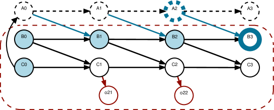
Figure 9: Impact of initial belief connectivity on the d-separating set of the IALM.

Now, to define the IALM, we will need the induced probability of $B^{3}$, which according to (4.7) can be written as

$$\Pr(B^{3}|\left\langle B^{2},{D}_{i}^{3}\right\rangle,{I}_{\rightarrow i}^{3})=\sum_{A^{2}}I(A^{2}|{D}_{i}^{3})\Pr(B^{3}|B^{2},A^{2}).$$

Therefore ${D}_{i}^{3}$ needs to contain any variables that can be used to better predict $A^{2}$ (more formally, any variables that d-separate $A^{2}$ from ${\vec{h}}_{i}^{t}$ and any remaining variables $x_{i}^{t}$, cf. Definition 11). However, looking at the figure, we see that this means that $C^{0}$ needs to be included in the d-set.

At the same time, however, we see that we do not need to condition on the entire history $\vec{C}^{t}$. This may appear counter intuitive, since observations at later time steps (e.g, ${o}_{i}^{1}$ and ${o}_{i}^{2}$) certainly provide information about $A^{2}$, while they also depend on $\vec{C}^{t}$. But this is precisely the point: by including $C^{0}$ in the d-separating set, it becomes part of the hidden state—e.g., for $t=2$ we have ${\bar{s}}_{i}^{2}=\langle{x}_{i}^{2},{D}_{i}^{3}\rangle=\langle\left\langle C^{2}\right\rangle,\left\langle B^{0},B^{1},B^{2},C^{0}\right\rangle\rangle$—and those later observations certainly provide information as to what that hidden state is.

4.3 Planning in an IALM

Here we look at how we can plan using an IALM. It turns out that this is surprisingly simple, since an IALM is a (special case of) POMDP.

Observation.

An influence-augmented local model is a POMDP.

Proof.

This can simply be verified by comparing Definition 15 to the definition of a POMDP (Definition 1).∎

This means that belief updates and definition of value functions follow as usual. For completeness and future reference, we write these out in detail below.

4.3.1 Local-form Belief Update

As implied by Definition 15, in an IALM, an agent uses a local-form belief:

Definition 17 (local-form belief).

A local-form belief ${b}_{i}^{l,{t}}$ for an IALM constructed for agent $i$ is the posterior probability distribution over augmented states ${\bar{s}}_{i}^{t}=\langle{x}_{i}^{t},{D}_{i}^{t+1}\rangle$.

The belief update for such a local-form belief is as in a regular POMDP, cf. (2.1):

$$BU({b}_{i}^{l},{a}_{i}^{t},{o}_{i}^{t+1})({\bar{s}}_{i}^{t+1})=\frac{1}{\Pr({o}_{i}^{t+1}|{b}_{i}^{l},{a}_{i}^{t})}\bar{O}_{i}({o}_{i}^{t+1}|{a}_{i}^{t},{\bar{s}}_{i}^{t+1})\sum_{{\bar{s}}_{i}^{t}}\bar{T}_{i}({\bar{s}}_{i}^{t+1}|{\bar{s}}_{i}^{t},{a}_{i}^{t}){b}_{i}^{l}({\bar{s}}_{i}^{t})=\\ \frac{O({o}_{i}^{t+1}|{a}_{i}^{t},{x}_{i}^{t+1})}{\Pr({o}_{i}^{t+1}|{b}_{i}^{l},{a}_{i}^{t})}\sum_{{x}_{i}^{t},{D}_{i}^{t+1}}\Pr({x}_{i}^{t+1}|\langle{x}_{i}^{t},{D}_{i}^{t+1}\rangle,{a}_{i}^{t},{I}_{\rightarrow i}^{t+1})\boldsymbol{1}_{\{{D}_{i}^{t+2},d({x}_{i}^{t},{a}_{i}^{t},{x}_{i}^{t+1},{D}_{i}^{t+1})\}}{b}_{i}^{l}({x}_{i}^{t},{D}_{i}^{t+1})$$ (4.10)

The expected observation probability (the normalization factor) in this case can be shown (see the derivation in Appendix A.3.1) to satisfy

$$\Pr({o}_{i}^{t+1}|{b}_{i}^{l},{a}_{i}^{t}) = \mathbf{E}_{{\bar{s}}_{i}^{t}\sim{b}_{i}^{l},{\bar{s}}_{i}^{t+1}\sim\bar{T}({\bar{s}}_{i}^{t},{a}_{i}^{t},\cdot)}\left[\bar{O}({o}_{i}^{t+1}|{a}_{i}^{t},{\bar{s}}_{i}^{t+1})\right]$$ (4.11)

$$= \mathbf{E}_{\left\langle{x}_{i}^{t},{D}_{i}^{t+1}\right\rangle\sim{b}_{i}^{l},\left\langle{x}_{i}^{t+1},{D}_{i}^{t+2}\right\rangle\sim\bar{T}(\left\langle{x}_{i}^{t},{D}_{i}^{t+1}\right\rangle,{a}_{i}^{t},\cdot)}\left[O({o}_{i}^{t+1}|{a}_{i}^{t},{x}_{i}^{t+1})\right]$$

$$= \sum_{{x}_{i}^{t+1}}O({o}_{i}^{t+1}|{a}_{i}^{t},{x}_{i}^{t+1})\Pr({x}_{i}^{t+1}|{b}_{i}^{l},{a}_{i}^{t},{I}_{\rightarrow i}^{t+1}),$$

with

$$\Pr({x}_{i}^{t+1}|{b}_{i}^{l},{a}_{i}^{t},{I}_{\rightarrow i}^{t+1})\operatorname{\triangleq}\sum_{{x}_{i}^{t},{D}_{i}^{t+1}}\Pr({x}_{i}^{t+1}|\langle{x}_{i}^{t},{D}_{i}^{t+1}\rangle,{a}_{i}^{t},{I}_{\rightarrow i}^{t+1}){b}_{i}^{l}({x}_{i}^{t},{D}_{i}^{t+1}).$$ (4.12)

4.3.2 IALM Value

Putting everything together, we can show that for an IALM, the value function is similar to the normal POMDP value function:

Proposition 2 (IALM value function).

The value function is given by

$${Q}_{i}^{t}({b}_{i}^{l},{a}_{i}^{t})={R}_{i}({b}_{i}^{l},{a}_{i}^{t})+\gamma\sum_{{o}_{i}^{t+1}}\Pr({o}_{i}^{t+1}|{b}_{i}^{l},{a}_{i}^{t}){V}_{i}^{t+1}(BU({b}_{i}^{l},{a}_{i}^{t},{o}_{i}^{t+1})),$$ (4.13)

$${V}_{i}^{t+1}({b}_{i}^{l})=\max_{{a}_{i}}{Q}_{i}^{t+1}({b}_{i}^{l},{a}_{i}),$$ (4.14)

where

$${R}_{i}({b}_{i}^{l},{a}_{i}^{t}) = \mathbf{E}_{{\bar{s}}_{i}^{t}\sim{b}_{i}^{l},{\bar{s}}_{i}^{t+1}\sim\bar{T}({\bar{s}}_{i}^{t},{a}_{i}^{t},\cdot)}\left[\bar{R_{i}}({\bar{s}}_{i}^{t},{a}_{i}^{t},{\bar{s}}_{i}^{t+1})\right]$$ (4.15)

$$= \sum_{{x}_{i}^{t}}\sum_{{x}_{i}^{t+1}}{R}_{i}({x}_{i}^{t},{a}_{i}^{t},{x}_{i}^{t+1})\Pr({x}_{i}^{t},{x}_{i}^{t+1}|{b}_{i}^{l},{a}_{i}^{t},{I}_{\rightarrow i}^{t+1})$$

with

$$\Pr({x}_{i}^{t},{x}_{i}^{t+1}|{b}_{i}^{l},{a}_{i}^{t},{I}_{\rightarrow i}^{t+1})\operatorname{\triangleq}\sum_{{D}_{i}^{t+1}}\Pr({x}_{i}^{t+1}|\langle{x}_{i}^{t},{D}_{i}^{t+1}\rangle,{a}_{i}^{t},{I}_{\rightarrow i}^{t+1}){b}_{i}^{l}({x}_{i}^{t},{D}_{i}^{t+1}).$$ (4.16)

Proof.

This follows from the value function of regular POMDPs together with the derivations of ${R}_{i}({b}_{i}^{l},{a}_{i}^{t})$ and $\Pr({x}_{i}^{t},{x}_{i}^{t+1}|{b}_{i}^{l},{a}_{i}^{t},{I}_{\rightarrow i}^{t+1})$ in Appendix A.3.2.∎

The solution of the IALM gives the influence-based best-response value, defined as the value of the initial local-form belief:

$${V}_{i}({I}_{\rightarrow i}({\pi}_{-{i}}))\operatorname{\triangleq}{V}_{i}^{0}({b}_{i}^{l,{0}}).$$ (4.17)

4.4 IBA by Example

To further clarify the process of influence-based abstraction, and provide some intuition of the potential computational savings and in which cases they could arise, we discuss two examples in some more detail.

The Planetary Exploration Domain.

First, let us consider the planetary rover domain illustrated in Figure 7. We will give a characterization of this problem in terms of number of states, for both the global-form best-response model (GFBRM) and IALM, thus providing an analysis of the computational savings that can arise in this case.

We will use the following notations and assumptions:

• $L$ is the number of locations

• $pl\in\left\{yes,no\right\}$ indicates if a plan has been sent to the rover.

• $B$ is the number of private states ${bt}_{1}$ of the satellite (e.g., number of battery levels).

• $\left|{\mathcal{O}}_{1}\right|$ is the size of the observation set of agent 1. In case that ${o}_{1}={bt}_{1}$, i.e., the satellite can perfectly observe its battery level, we would have $\left|{\mathcal{O}}_{1}\right|=B$.

• ${a}_{1}\in\left\{NOOP,\,PLAN\right\}$ is the action of the satellite.

So now, in the GFBRM model, the augmented state for the rover (who is agent 2) is ${\bar{s}}_{2}^{t}=\langle{s}^{t},{\vec{h}}_{1}^{t}\rangle=\langle{bt}_{1}^{t},{pl}^{t},{l}_{2}^{t},{\vec{h}}_{1}^{t}\rangle$. Given the above assumptions, the number of AOHs for the satellite at stage $t$ is $|{\vec{\mathcal{H}}}_{1}^{t}|=\left(2\left|{\mathcal{O}}_{1}\right|\right)^{t}$. And therefore the state space of the GFBRM is of size $\left|{\bar{\mathcal{S}}}_{i}^{t}\right|=2LB\cdot\left(2\left|{\mathcal{O}}_{1}\right|\right)^{t}$.

In contrast, in an IALM, we have states ${\bar{s}}_{2}^{t}=\langle{x}_{2}^{t},{D}_{2}^{t+1}\rangle=\left\langle\left\langle{pl}^{t},{l}_{2}^{t}\right\rangle,{pl}^{0:t}\right\rangle=\left\langle{l}_{2}^{t},{pl}^{0:t}\right\rangle$, meaning that the size of the state space in the IALM is $L\cdot 2^{t+1}$, which is strictly smaller than the GFBRM model.

Moreover, we can exploit that fact that $pl$ can only turn on, meaning that ${pl}^{0:t}$ has only $t+2$ possible values: it got turned on on one of the stages $0\dots t$ or it has not yet been turned on (“$NotYet$”). We refer to this re-coded variable as $PlanIssueTime^{t}=\sigma({pl}^{0:t})$ such that we can write ${\bar{s}}_{i}^{t}=\left\langle{l}_{2},PlanIssueTime^{t}\right\rangle$. This means that the number of IALM states at stage $t$ in the planetary exploration problem can be further reduced to $L\left(t+2\right)$. This suggests that the IALM will be much cheaper to solve for larger horizons: it scales linearly with $t$, whereas the GFBRM scales exponentially with $t$.

However, our discussion so far has excluded the time it takes to construct the IALM. Specifically, to compute the transition probabilities for every stage $t$, we will need to compute the incoming influence:

$$I({u}_{\rightarrow 1}^{t+1}|{D}_{1}^{t+1})=\Pr({a}_{1}^{t}|PlanIssueTime^{t}).$$

In general, we would need to compute this for all possible instantiations of ${D}_{2}^{t+1}$. However, in this case, the action of the satellite agent is only relevant in when $PlanIssueTime^{t}=NotYet$, which mean that we only need to compute the probability $\Pr({a}_{1}^{t}|PlanIssueTime^{t}=NotYet)$. Applying (4.4) yields (we leave ${{b}}^{0},{\pi}_{-{i}}$ implicit):

$$\Pr({a}_{1}^{t}|PlanIssueTime^{t})=\sum_{{\vec{h}}_{1}^{t}}{\pi}_{1}({a}_{1}^{t}|{\vec{h}}_{1}^{t})\Pr({\vec{h}}_{1}^{t}|PlanIssueTime^{t}),$$

which shows that if we have $\Pr({\vec{h}}_{1}^{t}|PlanIssueTime^{t})$ for each stage $t$, we can directly derive $\Pr({a}_{1}^{t}|PlanIssueTime^{t})$. The main issue therefore is to compute $\Pr({\vec{h}}_{1}^{t}|PlanIssueTime^{t})$ for all $t=1\dots h-1$. This is essentially a belief tracking problem. Specifically, we can model this as a special type of hidden Markov model where the hidden state is $\langle{bt}_{1}^{t},{\vec{h}}_{1}^{t}\rangle$, and our observations are ${pl}^{t}$. The number of such states at stage $t$ is $B\cdot\left(2\left|{\mathcal{O}}_{1}\right|\right)^{t}$ and that also is the dominant term in the complexity.

This shows that in this example, computing a best-response using a GFBRM requires to solve a POMDP with $\left|\mathcal{S}^{GFBR}\right|=2LB\cdot\left(2\left|{\mathcal{O}}_{1}\right|\right)^{t}$, while doing it using an IALM requires solving a POMDP with $\left|\mathcal{S}^{IALM}\right|=L\left(t+2\right)$ states and a construction cost of $O\left(B\cdot\left(2\left|{\mathcal{O}}_{1}\right|\right)^{t}\right)$. This means that particularly when also the number $L$ of locations is considerable, we can tackle much larger problems, since we have isolated the exponential complexity of tracking ${\vec{h}}_{1}^{t}$ from the impact of the number of locations $L$. Similarly, in the case where $B$ (in general the number of states induced by non-modeled factors) is very large, this cost now only appears in the IALM construction and is not multiplied with $L$.

The House Search Domain

Next, we turn to the House Search problem, illustrated in Figure 6. In contrast to Planetary Exploration, House Search exhibits a more substantial d-separating set ${D}_{2}^{t+1}$ and so we expect less computational savings. In fact, as we will see below, the IALM provides little to no computational benefit except in the face of additional assumptions on the structure of the problem.

Let us again define the sizes of the relevant quantities:

• $L$ is the number of locations.

• $f\in\left\{yes,no\right\}$ indicates if the target has been found. Once a target has been found the location ${l}_{1}$ of agent 1 no longer has any effect.

• $\left|{\mathcal{O}}_{1}\right|$ is the size of the observation set of agent 1. In case that ${o}_{1}=\left\langle{l}_{1},f\right\rangle$, i.e., the agent can perfectly observe its location and if the target is found, we would have $\left|{\mathcal{O}}_{1}\right|=2L$.

• ${\mathcal{A}}_{1}={\mathcal{A}}_{2}$ are the action sets that can allow the agents to move to adjacent rooms.

Repeating the analysis, we see that the GFBRM state is ${\bar{s}}_{2}^{t}=\langle{s}^{t},{\vec{h}}_{1}^{t}\rangle=\left\langle\left\langle{l}_{1}^{t},{f}^{t},{l}_{tgt}^{t},{l}_{2}^{t}\right\rangle,{\vec{h}}_{1}^{t}\right\rangle$. Since $|{\vec{\mathcal{H}}}_{1}^{t}|=\left(\left|{\mathcal{A}}_{1}\right|\left|{\mathcal{O}}_{1}\right|\right)^{t},$ the state space of the GFBRM is of size $\left|{\bar{\mathcal{S}}}^{t}\right|=2L^{3}\left(\left|{\mathcal{A}}_{1}\right|\left|{\mathcal{O}}_{1}\right|\right)^{t}$. If we assume the agent has 4 movement actions and can perfectly observe it location and if the target is found, as above, this becomes $2L^{3}\left(4\cdot 2L\right)^{t}=2L^{3}\left(8L\right)^{t}=2^{3t+1}L^{t+3}$.

On the other hand, the IALM has states ${\bar{s}}_{2}^{t}=\langle{x}_{2}^{t},{D}_{2}^{t+1}\rangle=\left\langle{f}^{0:t},{l}_{tgt}^{0:t},{l}_{2}^{0:t}\right\rangle$. Therefore, without further simplifications, the size of the state space at stage $t$ in the IALM is $2^{t+1}\cdot L^{2(t+1)}$. In other words, even disregarding the construction costs of the IALM, this would only guaranteed to be smaller for time step $t=1$, as illustrated in Table 1.

Simplifications are possible, however: as before, the ‘found’ variable $f$ may only turn on which reduces the IALM state to ${\bar{s}}_{2}^{t}=\left\langle foundTime^{t},{l}_{tgt}^{0:t},{l}_{2}^{0:t}\right\rangle$ and the state space size to $(t+2)\cdot L^{2(t+1)}$. When the target is stationary, this reduces to $(t+2)\cdot L\cdot L^{(t+1)}$. Also, it may not be realistic that all sequences of locations are realizable. Given a fixed start position and 4 deterministic movement actions, the number of realizable sequences of locations would be $O(4^{t}),$which would lead to a ‘simplified IALM’ with state space of size $(t+2)\cdot L\cdot 4^{t}$. Exploiting the realizable location sequences of agent $1$ to similarly reduce the state space of the GFBRM leads to $2\cdot L^{3}\cdot(t+2)\cdot 4^{t}$ states. As such, the IALM representation in terms of ${\bar{s}}_{2}^{t}=\langle{x}_{2}^{t},{D}_{2}^{t+1}\rangle$ enables us to capture structure of the problem to significantly reduce its local state space.

			stage $t$
model	state space size		$1$	$2$	3	4
GFBRM	$2^{3t+1}L^{t+3}$		$16L^{4}$	$128L^{5}$	$1024L^{6}$	$8192L^{7}$
GFBRM simplified	$2\cdot L^{3}\cdot(t+2)\cdot 4^{t}$		$24L^{3}$	$128L^{3}$	$640L^{3}$	$3072L^{3}$
IALM naive	$2^{t+1}\cdot L^{2(t+1)}$		$4L^{4}$	$8L^{6}$	$16L^{8}$	$32L^{10}$
IALM simplified	$L\cdot(t+2)\cdot 4^{t}$		$12L$	$64L$	$320L$	$1536L$

Table 1: State space sizes for GFBRM and two versions of IALM models for the House Search problem.

Of course, we did not yet cover the cost of the construction cost of the IALM by computing the influence. Here, we sketch what is involved in the construction of the ‘simplified IALM’ we constructed. Specifically the influence specification now is:

$$I({u}_{\rightarrow 1}^{t+1}|{D}_{1}^{t+1})=\Pr({l}_{1}^{t}|\left\langle FoundTime^{t},{l}_{tgt},{l}_{2}^{0:t-1}\right\rangle).$$

As before, we only care about cases where $FoundTime^{t}=NotYet$ (since otherwise the location ${l}_{1}^{t}$ is irrelevant). However, the different options for ${l}_{tgt},{l}_{2}^{0:t-1}$ should be evaluated, which means that we need to solve the inference problem for $O(L\cdot 4^{t-1})$ instantiations of the d-set. Each of these instantiations requires tracking hidden states of the form $\left\langle{l}_{1}^{t},{\vec{h}}_{1}^{t}\right\rangle$, and there are $L\left(\left|{\mathcal{A}}_{1}\right|\left|{\mathcal{O}}_{1}\right|\right)^{t}$ of them in general. For the simplified setting of deterministic moves and perfect observations by agent 1 this can be limited to $L\cdot t\cdot 4^{t}$ since in that case ${\vec{h}}_{1}^{t}=\left\langle{f}^{0:t},{l}_{1}^{0:t}\right\rangle=\left\langle FoundTime^{t},{l}_{1}^{0:t}\right\rangle$.

In summary, the simplified version of the House Search problem enables us to reduce the state space of the best-response model substantially, from $2^{3t+1}L^{t+3}$ to $L\cdot(t+2)\cdot 4^{t}$. However to construct the IALM state space at stage $t$ still requires time of the order $(L\cdot 4^{t-1})(L\cdot t\cdot 4^{t})=L^{2}\cdot t\cdot 4^{2t-1}$.

4.5 More General Implications of IBA

In the above, we saw that IBA can lead to more efficient computation of exact best-responses in settings that have sufficient structure to exploit. However, our motivation for developing the theory presented in this paper is more general than this. Here we elaborate on the broader implications that we envision.

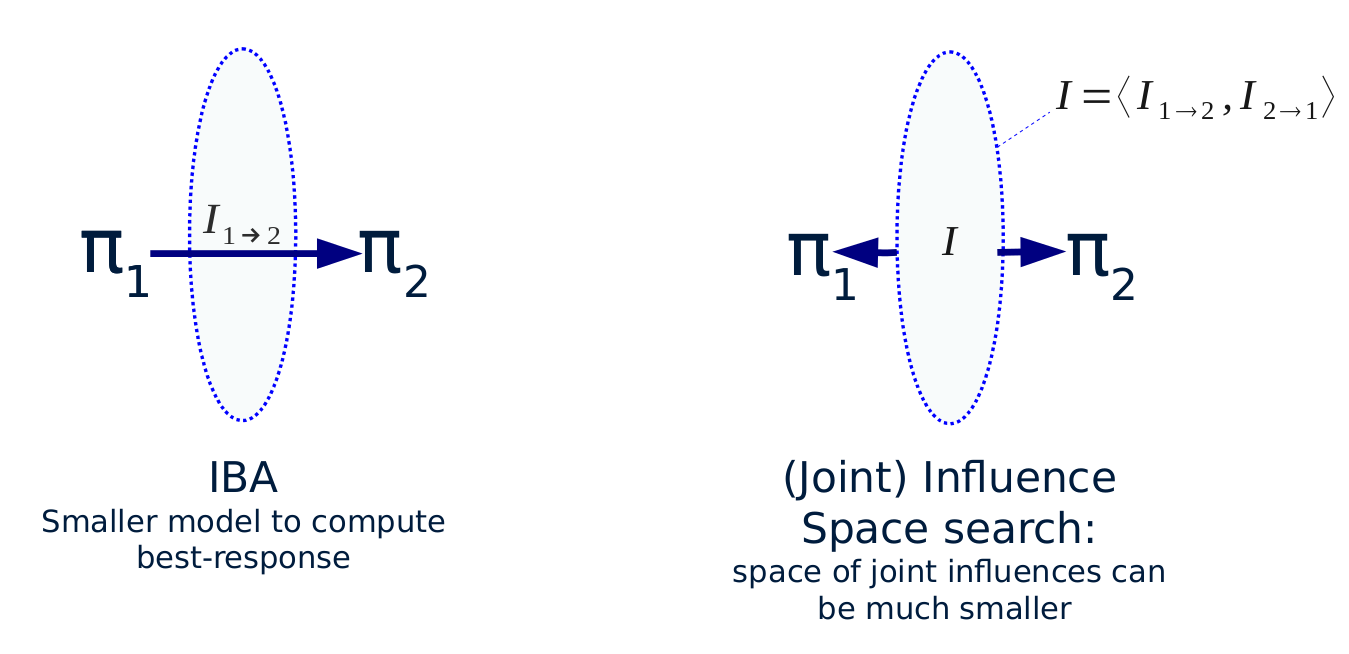
Figure 10: Illustration of the ideas of influence-based abstraction and influence search.

4.5.1 Influence Search

The ideas underlying influence-based abstraction were developed in the research community focusing on multiagent sequential decision making by people like ? (?), ? (?) and ? (?). The goal that these works pursued were not the computation of merely a best response, but of the optimal joint policy. Hence these works performed a type of influence search (?). The idea, illustrated in Figure 10, is that many policies of one agent, say agent $1$, may correspond to the same influence $I_{1\rightarrow 2}$ on agent $2$, which would mean that the set of such influences could be much smaller than the set of possible policies ${\pi}_{2}$. Therefore, if it is possible to search through the space of joint influences ${I}=\left\langle I_{1\rightarrow 2},I_{2\rightarrow 1}\right\rangle$, this could be much more effective than searching the much larger space of joint policies $\pi=\left\langle{\pi}_{1},{\pi}_{2}\right\rangle$. Specifically, ? (?) showed orders of improvement in computational cost over joint policy-search approaches.

So far, however, these ideas have only been exploited in sub-classes of fDec-POMDPs (see also Section 7), and generalizing influence search to general fDec-POMDPs or even fPOSG (i.e., to find Nash equilibria) is still an open problem. Our definition of influence in Definition 12 can serve as a starting point for such extensions.

4.5.2 Approximate Influence Representations

The discussion in Section 4.4 demonstrated that, in cases with sufficient structure, the representation of the influence $I({u}_{\rightarrow i}^{t+1}|{D}_{i}^{t+1})$ can be compact, leading to substantial benefits. However, at the same time it also showed that in general, without exploiting special properties of the domain, these representations can become very big and unwieldy due to the dependence on the history of a subset of variables. Large influence representations can not be exploited for more efficient best-response computations, and they also suggest that the number of possible influences will be large, possibly limiting the effectiveness of influence search.

However, even though exact representations of $I({u}_{\rightarrow i}^{t+1}|{D}_{i}^{t+1})$ may be very large, it might be the case that approximate representations $\hat{I}({u}_{\rightarrow i}^{t+1}|{D}_{i}^{t+1})$ can be compactly represented while still affording good performance; for the purposes of making good predictions it is usually not required to remember the full history (?, ?, ?, ?). Moreover, learning such approximate influence points is a supervised learning problem (a specific type of sequence prediction problem), which means that we can directly build on recent advancements for such prediction problems, including work on deep learning  (?, ?). Of course, whether the successes from natural language processing (?, ?), machine translation (?), speech recognition (?, ?) or biological sequence data (?) will transfer to the task of influence prediction remains to be investigated, but there already are some positive indications.

Specifically, some studies have shown that approximate representations of influence can enable further scalability in a variety of respects. For instance, ? (?) introduced the idea of transfer planning, which defines a number of smaller source tasks, whose solution is transferred to the larger (involving more agents) target task. The definition of the source tasks ignores the actual influence of the rest of the system, and hence can be seen as a very naive special case of approximate influence-based abstraction: it assumes an arbitrary influence point for each sub-problem. Nevertheless, the authors empirically showed that this can lead to good performance in Dec-POMDPs with many agents. This was corroborated by ? (?) who employed optimistic influences (also an approximate form of influence) to compute factored upper bounds on the Dec-POMDP value function. They demonstrated that in some cases the solution found by transfer planning for Dec-POMDPs with over 50 agents was essentially optimal. Recently, ? (?) demonstrated that, by using learned (recurrent neural network) representations of influence in online planning, it is possible to get better task performance when the time for action selection is limited. Of course, giving hard performance guarantees for such approaches is very difficult, but ? (?) show that it is possible to derive performance loss bounds for approximate influence representations. Their analysis also suggests that typical machine learning approaches that minimize the cross-entropy loss may be well aligned with minimizing the performance loss.

As such, there is substantial evidence that approximate extension of the formal IBA framework presented in this paper can lead to various benefits. Related to this is the new perspective these approaches give on the systems they aim to control. For instance, both ? (?) and ? (?) experimented with forms of “influence strength” to better understand parametrized domains by looking at the impact on the resulting solution quality. Further formalization and refinements of such notions could lead to a better understanding of the application of decision making methods to complex domains.

4.5.3 Identifying Inductive Biases

Notions like influence strength can enable us to better understand the problems that we are trying to tackle, and the IBA perspective can generate more of such insights. For instance, the discussion on the impact of the initial state distribution 4.2.3 neatly exemplifies some different types of structure we can expect to encounter when dealing with abstraction in structured decision making processes.

Identification of such structure is important even for deep learning: even though the representations are learned automatically, no learning methods are effective without the appropriate inductive biases (?, ?). For instance, convolutional neural networks are so successful for image processing because they exploit the fact that there is local and repeated structure in real-world images. In a similar way, in the discussion on the initial state distribution, we noticed that certain forms of structure, such as dependence on certain state factors at stage $t=0$, might be common in sequential decision processes involving abstraction.

In fact, recent research provides clear evidence that structure as implied by influence-based abstraction can be effectively used to bias deep reinforcement learning (?). Specifically, that work shows that by equipping a policy and/or value network with a recurrent sub-network that is only fed with a subset of variables (roughly corresponding to the d-separating set) can lead to higher performance than feed-forward networks, while learning much faster than a full-sized recurrent neural network. Further connections to deep RL and multiagent RL approaches are discussed in Section 8.

5 IBA With Intra-Stage Dependencies

The previous section presented the framework of influence-based abstraction, which enables us to abstract away hidden state variables in so-called local-form models. We illustrated how this can lead to speeding up best-response computations and discussed more general implications of the theory. So far we assumed there are no intra-stage connections: all influence links span a time step. However, intra-stage dependencies (ISDs) can be useful to specify a more intuitive model, as we saw for House Search in Figure 2a. Additionally, there could be problems that only have a correct formulation using intra-stage dependencies: since intra-stage connections can model additional correlations, the transition functions $T({s}^{t+1}|{s}^{t},{a}^{t})$ that can be represented without ISDs is a strict subset of those we can represent with ISDs. Simply removing ISDs from problems that need them is not possible, as it is not clear what probabilities the CPTs should specify for the remaining parents.

Moreover, intra-stage connections enable us to introduce ‘dummy’ variables, as discussed in Section 4.1.1. Without this capability, the requirement of including all observation-relevant and reward-relevant variables in the local state (cf. Definition 10) would limit the applicability of influence-based abstraction. For instance, imagine the setting where our agent’s reward is directly affected by how many other agents take the some action $a$. Without intra-stage connections, we would be forced to model all the action variables of the other agents in the local state, making the local model intractable. However, using intra-stage connections, we can instead introduce a count variable that affects our reward, while we do not model (abstract away) all the individual actions of other agents. As such, the ability to use ISDs can allow us to effectively describe scenarios with anonymous interactions, such as mean-field games and others (?, ?, ?, ?, ?, ?), in the IBA framework.

Therefore, this section extends our definition of influence to also be applicable for models that have such intra-stage dependencies (ISDs).

5.1 Definition of Influence under ISDs

Here we extend IBA by adapting notions of influence sources, d-separating sets, and incoming influence points to properly take into account ISDs.

5.1.1 Intra-Stage Influence Sources

In settings with intra-stage dependencies, there is at least one non-modeled factor ${y}^{t+1}$ that influences an NLAF ${\tilde{x}}^{t+1}$. If there are multiple such factors, we let ${y}_{u}^{t+1}$ denote them. Therefore, in order to perform IBA in settings with ISDs, we will need to predict influence sources ${u}_{\rightarrow i}^{t+1}=\left\langle{y}_{u}^{t},{a}_{u}^{t},{y}_{u}^{t+1}\right\rangle$. In order to correctly deal with the intra-stage sources ${y}_{u}^{t+1}$, we will additionally need to consider those variables that influence them.

Indirect Sources

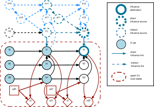
Figure 11: Illustration of the influence experienced by protagonist agent $i=2$ in the intra-stage version of House Search at stage $t=2$. ${f}^{2}$ is the influence destination, with direct influence source ${y}_{u}^{2}=\left\langle{l}_{1}^{2}\right\rangle$ (i.e., ${u}_{\rightarrow i}^{2}=\left\langle{l}_{1}^{2}\right\rangle$). Additionally, the figure highlights the indirect influence sources ${y}_{v}^{1}=\left\langle{l}_{1}^{1}\right\rangle$, ${a}_{v}^{t}=\left\langle{a}_{1}^{1}\right\rangle$ and $\vec{h}{}_{v}^{1}=\left\langle{\vec{h}}_{1}^{1}\right\rangle$, which determine the influence that is exerted at stage $t=1$. (Note that ${l}_{1}^{1}$ in fact is also a direct influence source for the influence experienced at stage $t=1$.)

In particular, we use ‘$v$’ as the symbol to denote such ‘indirect’ or ‘second order’ influences and will write ${x}_{v}^{t},{y}_{v}^{t},{a}_{i}^{t},{a}_{v}^{t},{x}_{v}^{t+1}$ and ${y}_{v}^{t+1}$ for the possible ancestors in the 2DBN of intra-stage sources ${y}_{u}^{t+1}$.

Example.

Figure  11 illustrates the direct and indirect influence sources for House Search. In order to be able to make accurate predictions of the influence destination ${f}^{2}$, at stage $t=1$ we should be able to predict ${l}_{1}^{1}\,({y}_{v}^{1})$ and ${a}_{1}^{1}\,({a}_{v}^{t})$ as accurately as possible. Given that we assume access to the policy of agent $1$, we can equivalently predict ${y}_{v}^{1}={l}_{1}^{1},\vec{h}{}_{v}^{1}={\vec{h}}_{1}^{1}$.

Now, in order to define the influence, we will need to consider the probability of such ${y}_{u}^{t+1}$ given variables that we know how to predict at stage $t$. In general it is given by:

$$\Pr({y}_{u}^{t+1}|{x}_{v}^{t},{y}_{v}^{t},{a}_{i}^{t},{a}_{v}^{t},{x}_{v}^{t+1})=\sum_{{y}_{v}^{t+1}}\Pr({y}_{u}^{t+1},{y}_{v}^{t+1}|{x}_{v}^{t},{y}_{v}^{t},{a}_{i}^{t},{a}_{v}^{t},{x}_{v}^{t+1}),$$ (5.1)

where:

• $\Pr({y}_{u}^{t+1},{y}_{v}^{t+1}|{x}_{v}^{t},{y}_{v}^{t},{a}_{i}^{t},{a}_{v}^{t},{x}_{v}^{t+1})$ is the product of CPTs of (both direct and indirect) intra-stage sources—in Figure  11 this is simply $\Pr({l}_{1}^{2}|{l}_{1}^{1},{a}_{1}^{1})$,

• ${x}_{v}^{t}$ are those state factors at stage $t$ (“in the left-hand slice of the 2DBN”) that are modeled by agent $i$, and are ancestor to an intra-stage influence source of agent $i$ at stage $t+1$ (“in the right-hand slice of the 2DBN”)—in Figure  11 no such variables exist,

• ${y}_{v}^{t}$ are those state factors in the left-hand slice of the 2DBN that are not modeled by agent $i$, but are ancestor to an influence destination of agent $i$—in Figure  11 this is ${l}_{1}^{1}$,

• ${x}_{v}^{t+1},$ ${y}_{v}^{t+1}$ are the modeled, respectively non-modeled state factors at state $t+1$ that are ancestors to an intra-stage influence source—in Figure  11 no such variables exist,

• ${a}_{i}^{t}$ might directly or indirectly affect an an intra-stage influence source, in which case it needs to be included in (5.1)—in Figure  11 this is not the case, and

• ${a}_{v}^{t}$ are the actions of other agents that are ancestors of an intra-stage influence source—in Figure  11 this is ${a}_{1}^{1}$.

We will also write ${\vec{h}}_{v}^{t}$ for the AOHs of the agents $v$ that correspond to ${a}_{v}^{t}$ (i.e., those agents of which the action is an ancestor in the 2DBN of an influence destination of agent $i$).

All sources

So far we have introduced notation using $u$ for direct sources and using $v$ for indirect sources. We will also want to consider the union of direct and indirect sources, and for these purposes we will write $w$. For example, we will write ${a}_{w}^{t}=\left\langle{a}_{u}^{t},{a}_{v}^{t}\right\rangle$ for the actions of agents that either directly or indirectly influence an influence destination.

5.1.2 The D-Separating Set

We now build on this insight to define the d-separating set in problems with intra-stage dependencies:

Definition 18 (d-separating set).

The d-separating set for agent $i$, ${D}_{i}$, is a subset of variables (state factors and/or actions), such that the history of these variables d-separates ${y}_{w}^{t},{\vec{h}}_{w}^{t}$ from ${x}_{i}^{t},{\vec{h}}_{i}^{t}$. I.e., it is defined in such a way that

$$\forall_{{y}_{w}^{t},{\vec{h}}_{w}^{t}}\qquad\Pr({y}_{w}^{t},{\vec{h}}_{w}^{t}|{x}_{i}^{t},{\vec{h}}_{i}^{t},{D}_{i}^{t+1},{{b}}^{0},{\pi}_{-{i}})=\Pr({y}_{w}^{t},{\vec{h}}_{w}^{t}|{D}_{i}^{t+1},{{b}}^{0},{\pi}_{-{i}}).$$ (5.2)

As before this should be interpreted to mean: ${D}_{i}^{t+1}$ d-separates ${y}_{w}^{t},{\vec{h}}_{w}^{t}$ from those parts of ${x}_{i}^{t},{\vec{h}}_{i}^{t}$ (i.e, of the local model) not contained in ${D}_{i}^{t+1}$.

Comparing Definition 18 with the earlier Definition 11, we see they are pleasingly similar; all that changed is that $u$’s have been replaced with $w$’s to now take into account the possibility of indirect sources.

5.1.3 Definition of Influence under ISDs

With this as background, we are now in position to define the concept of influence in all its generality:

Definition 19 (Experienced Influence under ISDs).

The influence experienced by agent $i$ at stage $t+1$ is a conditional probability distribution over the direct influence sources:

$$I({u}_{\rightarrow i}^{t+1}|{D}_{i}^{t+1},{x}_{v}^{t},{a}_{i}^{t},{x}_{v}^{t+1})\operatorname{\triangleq}\Pr(\left\langle{y}_{u}^{t},{a}_{u}^{t},{y}_{u}^{t+1}\right\rangle|{D}_{i}^{t+1},{x}_{v}^{t},{a}_{i}^{t},{x}_{v}^{t+1},{{b}}^{0},{\pi}_{-{i}})\\ =\sum_{\left\langle{y}_{v}^{t},{a}_{v}^{t},{y}_{v}^{t+1}\right\rangle}\Pr({y}_{u}^{t+1},{y}_{v}^{t+1}|{x}_{v}^{t},{y}_{v}^{t},{a}_{i}^{t},{a}_{v}^{t},{x}_{v}^{t+1})\sum_{{\vec{h}}_{w}^{t}}{\pi}_{w}({a}_{w}^{t}|{\vec{h}}_{w}^{t})\Pr({y}_{w}^{t},{\vec{h}}_{w}^{t}|{D}_{i}^{t+1},{{b}}^{0},{\pi}_{-{i}})$$ (5.3)

where

• $u$ denote (direct) influence sources;

• $v$ denote the (indirect) ‘second order’ sources;

• $w$ (as above) denotes the union of $u$ and $v$;

• $\Pr({y}_{u}^{t+1},{y}_{v}^{t+1}|{x}_{v}^{t},{y}_{v}^{t},{a}_{i}^{t},{a}_{v}^{t},{x}_{v}^{t+1})$ is the term necessary to predict the intra-stage sources. It is a term that consists of the product of CPTs;

• ${\pi}_{w}({a}_{w}^{t}|{\vec{h}}_{w}^{t})=\prod_{i\in w}{\pi}_{i}({a}_{i}^{t}|{\vec{h}}_{i}^{t})={\pi}_{u}({a}_{u}^{t}|{\vec{h}}_{u}^{t}){\pi}_{v}({a}_{v}^{t}|{\vec{h}}_{v}^{t})$ is the product of action probabilities according to the policies of the other agents that are relevant directly (the $u$) or indirectly for intra-stage sources (the $v$); and

• $\Pr({y}_{w}^{t},{\vec{h}}_{w}^{t}|{D}_{i}^{t+1},{{b}}^{0},{\pi}_{-{i}})=\Pr({y}_{u}^{t},{y}_{v}^{t},{\vec{h}}_{u}^{t},{\vec{h}}_{v}^{t}|{D}_{i}^{t+1},{{b}}^{0},{\pi}_{-{i}})$ predicts the non-modeled factors that are relevant directly (the $u$) or indirectly for intra-stage sources (the $v$), as well as the histories for the relevant agents.

Tying back to the example of Figure 11, (5.3) reduces to

$$I({l}_{1}^{2}|{D}_{2}^{2})=\sum_{{l}_{1}^{1},{a}_{1}^{1}}\Pr({l}_{1}^{2}|{l}_{1}^{1},{a}_{1}^{1})\sum_{{\vec{h}}_{1}^{1}}{\pi}_{1}({a}_{1}^{1}|{\vec{h}}_{1}^{1})\Pr({l}_{1}^{1},{\vec{h}}_{1}^{1}|{D}_{1}^{2},{{b}}^{0},{\pi}_{1}).$$

We use ${I}_{\rightarrow i}^{t+1}({\pi}_{-{i}})$ to denote the conditional distribution $I(\cdot|{D}_{i}^{t+1},{x}_{i}^{t},{a}_{i}^{t},{x}_{i}^{t+1})$.

We make a few observations:

• The term $\Pr({y}_{u}^{t+1},{y}_{v}^{t+1}|{x}_{v}^{t},{y}_{v}^{t},{a}_{i}^{t},{a}_{v}^{t},{x}_{v}^{t+1})$ can be simplified as given by (5.1), but it is important to keep in mind that this resulting term requires actual inference and is not the product of CPTs anymore.

• Note that, in many cases, we will consider other agents that use deterministic policies, however, we chose to give the more general description that also allows for stochastic policies. In case of deterministic policies, the summation over ${a}_{v}^{t}$ can be omitted, ${a}_{v/w}^{t}$ can be replaced by ${\pi}_{v/w}^{t}({\vec{o}}_{v/w}^{\,t})$, and ${\vec{h}}_{w}^{t}$ becomes ${\vec{o}}_{w}^{\,t}$ (?).

• The dependence of $I({u}_{\rightarrow i}^{t+1}|{D}_{i}^{t+1},{x}_{v}^{t},{a}_{i}^{t},{x}_{v}^{t+1})$ on ${a}_{i}^{t}$ is only needed when ${a}_{i}^{t}$ is an indirect source (i.e., it is an ancestor of ${y}_{u}^{t+1}\text{ or }{y}_{v}^{t+1}$).

5.1.4 Exerted vs. Experienced Influence

Here we make a reinterpretation of the experienced influence at stage $t+1$ as the result of the influence exerted at stage $t$ plus the effect of the intra-stage effects. While this does not fundamentally change anything about the definition of influence per Definition 19, it may provide some insight on the nature with which influence manifests itself in settings with intra-stage connections, and provide guidance for possible implementations.

In particular, it is possible to define a distribution, only in terms of variables at stage $t$, which acts as a sufficient statistic to predict the intra-stage source. The intuition is that the experienced influence, can be thought of as being induced by the exerted influence:

• Exerted Influence (at stage $t$):

  $$\Pr({y}_{w}^{t},{a}_{w}^{t}|{D}_{i}^{t+1},{{b}}^{0},{\pi}_{-{i}})=\Pr({y}_{u}^{t},{y}_{v}^{t},{a}_{u}^{t},{a}_{v}^{t}|{D}_{i}^{t+1},{{b}}^{0},{\pi}_{-{i}})\\ =\sum_{{\vec{h}}_{w}^{t}}{\pi}_{w}({a}_{w}^{t}|{\vec{h}}_{w}^{t})\Pr({y}_{w}^{t},{\vec{h}}_{w}^{t}|{D}_{i}^{t+1},{{b}}^{0},{\pi}_{-{i}}).$$ (5.4)

• Experienced Influence (at $t+1$):

  $$I({u}_{\rightarrow i}^{t+1}|{D}_{i}^{t+1},{x}_{v}^{t},{a}_{i}^{t},{x}_{v}^{t+1})=\Pr({y}_{u}^{t},{a}_{u}^{t},{y}_{u}^{t+1}|{D}_{i}^{t+1},{x}_{v}^{t},{x}_{v}^{t+1},{{b}}^{0},{\pi}_{-{i}})\\ =\sum_{\left\langle{y}_{v}^{t},{a}_{v}^{t},{y}_{v}^{t+1}\right\rangle}\Pr({y}_{u}^{t+1},{y}_{v}^{t+1}|{x}_{v}^{t},{y}_{v}^{t},{a}_{i}^{t},{a}_{v}^{t},{x}_{v}^{t+1})\Pr({y}_{w}^{t},{a}_{w}^{t}|{D}_{i}^{t+1},{{b}}^{0},{\pi}_{-{i}}).$$ (5.5)

This last equation (5.5) clearly demonstrates how the experienced influence is induced by the exerted influence. The notion of exerted influence (5.4) lays a clear link to IBA in settings without ISDs (cf. Equation 4.4) and is conceptually useful since it isolates which information needs to be retained for each stage $t$. As such, we expect that any practical implementations for computing the influence by means of filtering (belief tracking) (?, ?) would use this as the primary quantity of interest.

5.2 Influence-Augmented Local Model (IALM)

Here we define the influence-augmented local model under intra-stage connections. Looking at Definition 15, we can conclude that the only changes that we need to make involve the transition function (4.9).

In particular, we need to deal with the fact our definition of influence (5.3) can now be of the more complex form $I({u}_{\rightarrow i}^{t+1}|{D}_{i}^{t+1},{x}_{v}^{t},{a}_{i}^{t},{x}_{v}^{t+1})$, as given by (5.5). This means that the NLAF probability $\Pr({\tilde{x}}_{i}^{t+1}|\langle{x}_{i}^{t},{D}_{i}^{t+1}\rangle,{a}_{i}^{t},{I}_{\rightarrow i}^{t+1})$ given by (4.7) must be updated to deal with this new form, and this in turn implies that the definition of $\bar{T}_{i}({\bar{s}}_{i}^{t+1}|{\bar{s}}_{i}^{t},{a}_{i}^{t})$ per (4.9) needs to be updated too.

Let us start with the former. Like (3.12), this can now depend on ISDs from OLAFs ${\mathring{x}}_{i}^{t+1}$

$$\Pr({\tilde{x}}_{i}^{t+1}|\langle{x}_{i}^{t},{D}_{i}^{t+1}\rangle,{\mathring{x}}_{i}^{t+1},{a}_{i}^{t},{I}_{\rightarrow i}^{t+1})\operatorname{\triangleq}\\ \sum_{{u}_{\rightarrow i}^{t+1}=\left\langle{y}_{u}^{t},{a}_{u}^{t},{y}_{u}^{t+1}\right\rangle}I({u}_{\rightarrow i}^{t+1}|{D}_{i}^{t+1},{x}_{v}^{t},{a}_{i}^{t},{x}_{v}^{t+1})\Pr({\tilde{x}}_{i}^{t+1}|{x}_{i}^{t},{\mathring{x}}_{i}^{t+1},{a}_{i}^{t},{u}_{\rightarrow i}^{t+1}),$$ (5.6)

with $\Pr({\tilde{x}}_{i}^{t+1}|{x}_{i}^{t},{\mathring{x}}_{i}^{t+1},{a}_{i}^{t},{u}_{\rightarrow i}^{t+1})$ simply the product of CPTs of the NLAFs, as given by (3.12), but now restricted to only ${y}_{i}^{t},{y}_{i}^{t+1},{a}_{-{i}}^{t}$ that are influence sources.

We are now in the position to define the IALM under intra-stage dependencies:

Definition 20 (IALM).

Given an LFM with intra-stage dependencies, $\mathcal{M}^{LFM}$, and profile of policies for other agents ${\pi}_{-{i}}$, an Influence-Augmented Local Model (IALM) for agent $i$ is a POMDP $\mathcal{M}_{i}^{IALM}(\mathcal{M}^{LFM},{\pi}_{-{i}})=\left\langle\bar{\mathcal{S}},{\mathcal{A}}_{i},\bar{T}_{i},\bar{R}_{i},{\mathcal{O}}_{i},\bar{O}_{i},H,{b}_{i}^{l,{0}}\right\rangle$, where

• $\bar{\mathcal{S}},{\mathcal{A}}_{i},\bar{R}_{i},{\mathcal{O}}_{i},\bar{O}_{i},H,{b}_{i}^{l,{0}}$ are identical to those in Definition 15,

• $\bar{T}_{i}$ is the transition function is defined as:

$$\bar{T}_{i}({\bar{s}}_{i}^{t+1}|{\bar{s}}_{i}^{t},{a}_{i}^{t})\operatorname{\triangleq}\Pr({x}_{i}^{t+1}|\langle{x}_{i}^{t},{D}_{i}^{t+1}\rangle,{a}_{i}^{t},{I}_{\rightarrow i}^{t+1})\boldsymbol{1}_{\{{D}_{i}^{t+2},d({x}_{i}^{t},{a}_{i}^{t},{x}_{i}^{t+1},{D}_{i}^{t+1})\}}\\ =\Pr({\tilde{x}}_{i}^{t+1}|\langle{x}_{i}^{t},{D}_{i}^{t+1}\rangle,{\mathring{x}}_{i}^{t+1},{a}_{i}^{t},{I}_{\rightarrow i}^{t+1})\Pr({\mathring{x}}_{i}^{t+1}|{x}_{i}^{t},{\tilde{x}}_{i}^{t+1},{a}_{i}^{t})\boldsymbol{1}_{\{{D}_{i}^{t+2},d({x}_{i}^{t},{a}_{i}^{t},{x}_{i}^{t+1},{D}_{i}^{t+1})\}},$$ (5.7)

with the first term is given by (5.6) and the second term is given by (3.11).

5.3 Planning in an IALM with ISDs

Since the only modifications that we needed to make to incorporate ISDs were in the transition function, the conclusions about how to plan in IALM made in Section 4.3 remain valid. In particular, the IALM is still a POMDP, with a well-defined belief-update function, and value functions. The solution of the IALM still gives the influence-based best-response value, defined in (4.17) as the value of the initial local-form belief: ${V}_{i}({I}_{\rightarrow i}({\pi}_{-{i}}))\operatorname{\triangleq}{V}_{i}^{0}({b}_{i}^{l,{0}}).$

6 Sufficiency of Influence-Based Abstraction

In this section, we will show that influence-based abstraction is completely lossless. By that we mean that an IALM constructed according to Definition 20 can be used to accurately predict rewards and observations, and thus to compute an exact, optimal (best-response) value.

The latter is our main result, Theorem 1, which shows that the optimal values for the GFBRM and the IALM are equal, thus establishing that one can use the IALM to plan (or learn) without any loss in value. In other words, it proves that the definition of influence constitutes a sufficient statistic for predicting the optimal value, and thus that the resulting IALM achieves a best-response against the policy ${\pi}_{-{i}}$ that generated the influence ${I}_{\rightarrow i}({\pi}_{-{i}})$.

Theorem 1.

For a finite-horizon POSG, the solution of the IALM for the incoming influence point ${I}_{\rightarrow i}({\pi}_{-{i}})$ associated with any ${\pi}_{-{i}}$ achieves the same value $V_{i}({I}_{\rightarrow i}({\pi}_{-{i}}))$, given by (4.17), as the best-response value $V_{i}({\pi}_{-{i}})$, given by (3.7), computed against ${\pi}_{-{i}}$ directly:

$$\forall_{{\pi}_{-{i}}}\quad V_{i}({I}_{\rightarrow i}({\pi}_{-{i}}))=V_{i}({\pi}_{-{i}}).$$ (6.1)

We note that this results also holds in the presence of intra-stage connections. To prove the result (in Section 6.4) we will show that the immediate reward terms and observation probabilities are equal (Section 6.3). In turn, to show this, we will need to show that transition probabilities are the same given a local-form belief and a global-form belief, which means that the local-form belief is a sufficient statistic to predict the next local state (Section 6.2). In order to allow the rewriting to take place, we first show how the global-form belief can be factorized.

We believe that this proof by itself is useful: it isolates the core technical property that needs to hold for sufficiency in Lemma 1 in Section 6.2. In this way it 1) conveys insight into the nature of how abstraction of latent state factors affects value, 2) provides a derivation that can be used to obtain simplifications of the definition of influence (Definition 19) in simpler cases, and 3) provides a recipe of how to prove similar results in problems which add even more complexities.

6.1 Factorization of the Global-Form Belief

In order to prove the equivalence of the GFBRM and the IALM, we will show that their value functions are the same. In order to do that, it will be necessary to decompose the global-form belief ${b}_{i}^{g}$ in components.

To do that, we make use of the insight that, for any ${D}_{i}^{t+1}$, the law of total probability allows us to write

$${b}_{i}^{g}({s}^{t},{\vec{h}}_{-{i}}^{t})=\sum_{{D}_{i}^{t+1}}{{b}}_{i}(\left\langle{x}_{i}^{t},{y}_{i}^{t}\right\rangle,{\vec{h}}_{-{i}}^{t},{D}_{i}^{t+1})=\sum_{{D}_{i}^{t+1}}{{b}}_{i}({x}_{i}^{t},{D}_{i}^{t+1}){{b}}_{i}({y}_{i}^{t},{\vec{h}}_{-{i}}^{t}|{x}_{i}^{t},{D}_{i}^{t+1}).$$ (6.2)

(We drop the superscript ‘g’ because we are rewriting to something that we do not call global-form belief anymore.)

Also, it is important to remember that the belief is defined as

$${b}_{i}^{g}({s}^{t},{\vec{h}}_{-{i}}^{t})\operatorname{\triangleq}\Pr({s}^{t},{\vec{h}}_{-{i}}^{t}|{\vec{h}}_{i}^{t},{{b}}^{0},{\pi}_{-{i}}),$$

which means that in (6.2), the definitions of the components are

$${{b}}_{i}({x}_{i}^{t},{D}_{i}^{t+1}) \operatorname{\triangleq} \Pr({x}_{i}^{t},{D}_{i}^{t+1}|{\vec{h}}_{i}^{t},{{b}}^{0},{\pi}_{-{i}}),$$ (6.3)

$${{b}}_{i}({y}_{i}^{t},{\vec{h}}_{-{i}}^{t}|{x}_{i}^{t},{D}_{i}^{t+1}) \operatorname{\triangleq} \Pr({y}_{i}^{t},{\vec{h}}_{-{i}}^{t}|{x}_{i}^{t},{D}_{i}^{t+1},{\vec{h}}_{i}^{t},{{b}}^{0},{\pi}_{-{i}}).$$ (6.4)

These equations further clarify how to think about inclusion of actions ${a}_{i}$ and observations ${o}_{i}$ inside the d-separating set ${D}_{i}^{t+1}$: the belief per definition conditions on the history of actions and observations, as such these can be included in ${D}_{i}^{t+1}$ without further problems. In particular, suppose that $a_{i}^{k}$ is part of d-separating set ${D}_{i}^{t+1}$, then this will lead to $\Pr({x}_{i}^{t},\left\langle\dots a_{i}^{k}\dots\right\rangle|\left\langle\dots a_{i}^{k}\dots\right\rangle,{{b}}^{0},{\pi}_{-{i}})$ in (6.4). However, the interpretation is simply that this does not influence the probabilities, since $P(x|x)=1$. Similarly, it would lead to a term $\Pr({y}_{i}^{t},{\vec{h}}_{-{i}}^{t}|{x}_{i}^{t},\left\langle\dots a_{i}^{k}\dots\right\rangle,\left\langle\dots a_{i}^{k}\dots\right\rangle,{{b}}^{0},{\pi}_{-{i}})$ in (6.4). Again, this poses no problem, since $\Pr(y|x,x)=\Pr(y|x)$. However, let us repeat that we do need all observation relevant state factors in the local state: otherwise we cannot define the local observation model $\bar{O}_{i}$ and track the local-form belief ${{b}}_{i}({x}_{i}^{t},{D}_{i}^{t+1})$ (cf. Definition 10 and Definition 15).

6.2 Sufficiency for Prediction of Local State Transitions

In this section, we show that the influence together with the local-form belief is sufficient to predict local state transitions. We first prove the following lemma, that shows that pairwise marginal distributions over states are the same in the IALM and the GFBRM. This will then be used in other proofs.

Lemma 1.

The joint distribution over current local state and next local state induced by a local-form belief is identical to that of the global-form belief:

$$\forall_{{\vec{h}}_{i}^{t}}\forall_{{x}_{i}^{t},{x}_{i}^{t+1}}\qquad\Pr({x}_{i}^{t},{x}_{i}^{t+1}|{b}_{i}^{g},{a}_{i}^{t},{\pi}_{-{i}})=\Pr({x}_{i}^{t},{x}_{i}^{t+1}|{b}_{i}^{l},{a}_{i}^{t},{I}_{\rightarrow i}^{t+1}),$$ (6.5)

where ${b}_{i}^{l},\,{b}_{i}^{g}$ denote the for the local-form and global-form beliefs induced by ${\vec{h}}_{i}^{t}$.

Proof.

To improve readability we will omit some time indices that do not cause confusion. We assume arbitrary ${\vec{h}}_{i}^{t},{x}_{i}^{t},{x}_{i}^{t+1}$, and start with the left-hand side, which is given by (3.15):

$$\sum_{{y}_{i}^{t}}\sum_{{a}_{-{i}}}\Pr({x}_{i}^{t+1}|{s}^{t},{a}_{i},{a}_{-{i}})\sum_{{\vec{h}}_{-{i}}^{t}}\Pr({a}_{-{i}}|{\vec{h}}_{-{i}}^{t},{\pi}_{-{i}}){b}_{i}^{g}({s}^{t},{\vec{h}}_{-{i}}^{t})$$

$$=$$ {via (6.2)}

$$\sum_{{y}_{i}^{t}}\sum_{{a}_{-{i}}}\Pr({x}_{i}^{t+1}|{s}^{t},{a}_{i},{a}_{-{i}})\sum_{{\vec{h}}_{-{i}}^{t}}\Pr({a}_{-{i}}|{\vec{h}}_{-{i}}^{t},{\pi}_{-{i}})\left[\sum_{{D}_{i}^{t+1}}{{b}}_{i}({x}_{i}^{t},{D}_{i}^{t+1}){{b}}_{i}({y}_{i}^{t},{\vec{h}}_{-{i}}^{t}|{x}_{i}^{t},{D}_{i}^{t+1})\right]$$ (6.6)

$$=$$ {via (3.9)}

$$\sum_{{y}_{i}^{t}}\sum_{{a}_{-{i}}}\left[\sum_{{y}_{i}^{t+1}}\Pr({y}_{i}^{t+1},{x}_{i}^{t+1}|{s}^{t},{a}_{i},{a}_{-{i}})\right]\sum_{{\vec{h}}_{-{i}}^{t}}\Pr({a}_{-{i}}|{\vec{h}}_{-{i}}^{t},{\pi}_{-{i}})\sum_{{D}_{i}^{t+1}}{{b}}_{i}({x}_{i}^{t},{D}_{i}^{t+1}){{b}}_{i}({y}_{i}^{t},{\vec{h}}_{-{i}}^{t}|{x}_{i}^{t},{D}_{i}^{t+1})$$ (6.7)

$$=$$ {via (3.10)}

$$\sum_{{y}_{i}^{t}}\sum_{{a}_{-{i}}}\sum_{{y}_{i}^{t+1}}\Pr({\mathring{x}}_{i}^{t+1}|{x}_{i}^{t},{a}_{i},{\tilde{x}}_{i}^{t+1})\Pr({\tilde{x}}_{i}^{t+1}|{x}_{i}^{t},{\mathring{x}}_{i}^{t+1},{a}_{i},{y}_{u}^{t},{y}_{u}^{t+1},{a}_{u})\Pr({y}_{i}^{t+1}|{x}_{i}^{t},{y}_{i}^{t},{a}_{i},{a}_{-{i}},{x}_{i}^{t+1})$$

$$\sum_{{\vec{h}}_{-{i}}^{t}}\Pr({a}_{-{i}}|{\vec{h}}_{-{i}}^{t},{\pi}_{-{i}})\sum_{{D}_{i}^{t+1}}{{b}}_{i}({x}_{i}^{t},{D}_{i}^{t+1}){{b}}_{i}({y}_{i}^{t},{\vec{h}}_{-{i}}^{t}|{x}_{i}^{t},{D}_{i}^{t+1})$$ (6.8)

$$=$$ {reordering terms}

$$\sum_{{D}_{i}^{t+1}}\Pr({\mathring{x}}_{i}^{t+1}|{x}_{i}^{t},{a}_{i},{\tilde{x}}_{i}^{t+1}){{b}}_{i}({x}_{i}^{t},{D}_{i}^{t+1})$$

$$\left[\sum_{{a}_{-{i}}}\sum_{{\vec{h}}_{-{i}}^{t}}\sum_{{y}_{i}^{t}}\sum_{{y}_{i}^{t+1}}\Pr({\tilde{x}}_{i}^{t+1}|{x}_{i}^{t},{\mathring{x}}_{i}^{t+1},{a}_{i},{y}_{u}^{t},{y}_{u}^{t+1},{a}_{u})\Pr({y}_{i}^{t+1}|{x}_{i}^{t},{y}_{i}^{t},{a}_{i},{a}_{-{i}},{x}_{i}^{t+1})\Pr({a}_{-{i}}|{\vec{h}}_{-{i}}^{t},{\pi}_{-{i}}){{b}}_{i}({y}_{i}^{t},{\vec{h}}_{-{i}}^{t}|{x}_{i}^{t},{D}_{i}^{t+1})\right]$$ (6.9)

This equation has grouped together all the probabilities that are affected by the non-local part of the problem in between the brackets. The terms before do not depend on the external part at all. We will now further investigate the externally influenced (bracketed) part:

$$\sum_{{a}_{-{i}}}\sum_{{\vec{h}}_{-{i}}^{t}}\sum_{{y}_{i}^{t}}\sum_{{y}_{i}^{t+1}}\Pr({\tilde{x}}_{i}^{t+1}|{x}_{i}^{t},{\mathring{x}}_{i}^{t+1},{a}_{i},{u}_{\rightarrow i}^{t+1})\Pr({y}_{i}^{t+1}|{x}_{i}^{t},{y}_{i}^{t},{a}_{i},{a}_{-{i}},{x}_{i}^{t+1}){\pi}_{-{i}}({a}_{-{i}}|{\vec{h}}_{-{i}}^{t}){{b}}_{i}({y}_{i}^{t},{\vec{h}}_{-{i}}^{t}|{x}_{i}^{t},{D}_{i}^{t+1})$$ (6.10)

$$= \sum_{{a}_{-{i}}}\sum_{{y}_{i}^{t}}\sum_{{y}_{i}^{t+1}}\Pr({\tilde{x}}_{i}^{t+1}|{x}_{i}^{t},{\mathring{x}}_{i}^{t+1},{a}_{i},{u}_{\rightarrow i}^{t+1})\Pr({y}_{i}^{t+1}|{x}_{i}^{t},{y}_{i}^{t},{a}_{i},{a}_{-{i}},{x}_{i}^{t+1})\sum_{{\vec{h}}_{-{i}}^{t}}{\pi}_{-{i}}({a}_{-{i}}|{\vec{h}}_{-{i}}^{t}){{b}}_{i}({y}_{i}^{t},{\vec{h}}_{-{i}}^{t}|{x}_{i}^{t},{D}_{i}^{t+1})$$ (6.11)

In this equation, not all non-modeled factors ${y}_{i}^{t+1}$ are relevant: we can restrict to the intra-stage sources ${y}_{u}^{t+1}$ and their intra-stage ancestors ${y}_{v}^{t+1}$, other factor’s probabilities just sum to 1. This yields:

$$\sum_{{a}_{-{i}}}\sum_{{y}_{i}^{t}}\sum_{{y}_{u}^{t+1}}\Pr({\tilde{x}}_{i}^{t+1}|{x}_{i}^{t},{\mathring{x}}_{i}^{t+1},{a}_{i},{u}_{\rightarrow i}^{t+1})\sum_{{y}_{v}^{t+1}}\Pr({y}_{u}^{t+1},{y}_{v}^{t+1}|{x}_{i}^{t},{y}_{i}^{t},{a}_{i},{a}_{-{i}},{x}_{i}^{t+1})\sum_{{\vec{h}}_{-{i}}^{t}}{\pi}_{-{i}}({a}_{-{i}}|{\vec{h}}_{-{i}}^{t}){{b}}_{i}({y}_{i}^{t},{\vec{h}}_{-{i}}^{t}|{x}_{i}^{t},{D}_{i}^{t+1})$$ (6.12)

$$= {a}_{v},{x}_{v}^{t+1} {y}_{u}^{t+1} v$$ {restricting to that actually influence . I.e.,   denotes other ‘second order’ sources}

$$\sum_{{a}_{-{i}}}\sum_{{y}_{i}^{t}}\sum_{{y}_{u}^{t+1}}\Pr({\tilde{x}}_{i}^{t+1}|{x}_{i}^{t},{\mathring{x}}_{i}^{t+1},{a}_{i},{u}_{\rightarrow i}^{t+1})\sum_{{y}_{v}^{t+1}}\Pr({y}_{u}^{t+1},{y}_{v}^{t+1}|{x}_{v}^{t},{y}_{v}^{t},{a}_{i},{a}_{v},{x}_{v}^{t+1})\sum_{{\vec{h}}_{-{i}}^{t}}{\pi}_{-{i}}({a}_{-{i}}|{\vec{h}}_{-{i}}^{t}){{b}}_{i}({y}_{i}^{t},{\vec{h}}_{-{i}}^{t}|{x}_{i}^{t},{D}_{i}^{t+1})$$

$$= {u}_{\rightarrow i}^{t+1}=\left\langle{y}_{u}^{t},{a}_{u},{y}_{u}^{t+1}\right\rangle$$ {pushing in summations, recall }

$$\sum_{{u}_{\rightarrow i}^{t+1}}\Pr({\tilde{x}}_{i}^{t+1}|{x}_{i}^{t},{\mathring{x}}_{i}^{t+1},{a}_{i},{u}_{\rightarrow i}^{t+1})\sum_{{a}_{v}}\sum_{{y}_{v}^{t}}\sum_{{y}_{v}^{t+1}}\Pr({y}_{u}^{t+1},{y}_{v}^{t+1}|{x}_{v}^{t},{y}_{v}^{t},{a}_{i},{a}_{v},{x}_{v}^{t+1})\sum_{{\vec{h}}_{-{i}}^{t}}{\pi}_{-{i}}({a}_{-{i}}|{\vec{h}}_{-{i}}^{t}){{b}}_{i}({y}_{i}^{t},{\vec{h}}_{-{i}}^{t}|{x}_{i}^{t},{D}_{i}^{t+1})$$ (6.13)

$$=$$ {marginalize out non-relevant terms}

$$\sum_{{u}_{\rightarrow i}^{t+1}}\Pr({\tilde{x}}_{i}^{t+1}|{x}_{i}^{t},{\mathring{x}}_{i}^{t+1},{a}_{i},{u}_{\rightarrow i}^{t+1})\sum_{{a}_{v}}\sum_{{y}_{v}^{t}}\sum_{{y}_{v}^{t+1}}\Pr({y}_{u}^{t+1},{y}_{v}^{t+1}|{x}_{v}^{t},{y}_{v}^{t},{a}_{i},{a}_{v},{x}_{v}^{t+1})$$

$$\sum_{{\vec{h}}_{u}^{t}}\sum_{{\vec{h}}_{v}^{t}}{\pi}_{u}({a}_{u}^{t}|{\vec{h}}_{u}^{t}){\pi}_{v}({a}_{v}^{t}|{\vec{h}}_{v}^{t}){{b}}_{i}({y}_{u}^{t},{y}_{v}^{t},{\vec{h}}_{u}^{t},{\vec{h}}_{v}^{t}|{x}_{i}^{t},{D}_{i}^{t+1})$$ (6.14)

$$= w=u\cup v$$ {let denote the union of direct and indirect sources}

$$\sum_{{u}_{\rightarrow i}^{t+1}}\Pr({\tilde{x}}_{i}^{t+1}|{x}_{i}^{t},{\mathring{x}}_{i}^{t+1},{a}_{i},{u}_{\rightarrow i}^{t+1})\sum_{{a}_{v}}\sum_{{y}_{v}^{t}}\sum_{{y}_{v}^{t+1}}\Pr({y}_{u}^{t+1},{y}_{v}^{t+1}|{x}_{v}^{t},{y}_{v}^{t},{a}_{i},{a}_{v},{x}_{v}^{t+1})\sum_{{\vec{h}}_{w}^{t}}{\pi}_{w}({a}_{w}|{\vec{h}}_{w}^{t},{\pi}_{w}){{b}}_{i}({y}_{w}^{t},{\vec{h}}_{w}^{t}|{x}_{i}^{t},{D}_{i}^{t+1})$$ (6.15)

$$= {{b}}_{i}({y}_{w}^{t},{\vec{h}}_{w}^{t}|{x}_{i}^{t},{D}_{i}^{t+1})\operatorname{\triangleq}\Pr({y}_{w}^{t},{\vec{h}}_{w}^{t}|{x}_{i}^{t},{D}_{i}^{t+1},{\vec{h}}_{i}^{t},{{b}}^{0},{\pi}_{-{i}})\overset{\text{\{def. of d-set \eqref{eq:dset-def--intrastage}}\}}{=}\Pr({y}_{w}^{t},{\vec{h}}_{w}^{t}|{D}_{i}^{t+1},{{b}}^{0},{\pi}_{-{i}})$$ {since }

$$\sum_{{u}_{\rightarrow i}^{t+1}}\Pr({\tilde{x}}_{i}^{t+1}|{x}_{i}^{t},{\mathring{x}}_{i}^{t+1},{a}_{i},{u}_{\rightarrow i}^{t+1})\sum_{\left\langle{y}_{v}^{t},{a}_{v},{y}_{v}^{t+1}\right\rangle}\Pr({y}_{u}^{t+1},{y}_{v}^{t+1}|{x}_{v}^{t},{y}_{v}^{t},{a}_{i},{a}_{v},{x}_{v}^{t+1})\sum_{{\vec{h}}_{w}^{t}}{\pi}_{w}({a}_{w}|{\vec{h}}_{w}^{t})\Pr({y}_{w}^{t},{\vec{h}}_{w}^{t}|{D}_{i}^{t+1},{{b}}^{0},{\pi}_{-{i}}).$$ (6.16)

We can now apply the definition of influence (Definition 19 19) to (6.16), which yields

$$=\sum_{{u}_{\rightarrow i}^{t+1}=\left\langle{y}_{u}^{t},{a}_{u},{y}_{u}^{t+1}\right\rangle}\Pr({\tilde{x}}_{i}^{t+1}|{x}_{i}^{t},{\mathring{x}}_{i}^{t+1},{a}_{i},{y}_{u}^{t},{a}_{u},{y}_{u}^{t+1})I({u}_{\rightarrow i}^{t+1}|{D}_{i}^{t+1},{x}_{v}^{t},{a}_{i},{x}_{v}^{t+1}),$$ (6.17)

which is the definition (5.6) of $\Pr({\tilde{x}}_{i}^{t+1}|\langle{x}_{i}^{t},{D}_{i}^{t+1}\rangle,{\mathring{x}}_{i}^{t+1},{a}_{i},{I}_{\rightarrow i}^{t+1})$.

Substituting (6.17) back in (6.9) we get

$$\sum_{{D}_{i}^{t+1}}\Pr({\mathring{x}}_{i}^{t+1}|{x}_{i}^{t},{x}_{i}^{t+1},{\tilde{x}}_{i}^{t+1},{a}_{i}){{b}}_{i}({x}_{i}^{t},{D}_{i}^{t+1})\left[\Pr({\tilde{x}}_{i}^{t+1}|\langle{x}_{i}^{t},{D}_{i}^{t+1}\rangle,{\mathring{x}}_{i}^{t+1},{a}_{i},{I}_{\rightarrow i}^{t+1})\right]$$

$$=$$ {via 5.7 }

$$\sum_{{D}_{i}^{t+1}}\Pr({x}_{i}^{t+1}|{x}_{i}^{t},{D}_{i}^{t+1},{a}_{i},{I}_{\rightarrow i}^{t+1}){{b}}_{i}({x}_{i}^{t},{D}_{i}^{t+1})\overset{\text{\{via \eqref{eq:P_xmxm_lfb}\}}}{=}\Pr({x}_{i}^{t},{x}_{i}^{t+1}|{b}_{i}^{l},{a}_{i}^{t},{I}_{\rightarrow i}^{t+1}),$$ (6.18)

which concludes the proof.∎

Lemma 2.

A local-form belief is a sufficient statistic for predicting the next local state. That is, when ${b}_{i}^{l},\,{b}_{i}^{g}$ denote the for the local-form and global-form beliefs induced by the same action-observation history ${\vec{h}}_{i}^{t}$, we have that:

$$\forall_{{\vec{h}}_{i}^{t}}\forall_{{x}_{i}^{t+1}}\qquad\Pr({x}_{i}^{t+1}|{b}_{i}^{g},{a}_{i}^{t},{\pi}_{-{i}})=\Pr({x}_{i}^{t+1}|{b}_{i}^{l},{a}_{i}^{t},{I}_{\rightarrow i}^{t+1}).$$ (6.19)

Proof.

This follows directly from Lemma (1):

$$\Pr({x}_{i}^{t+1}|{b}_{i}^{l},{a}_{i}^{t},{I}_{\rightarrow i}^{t+1})=\sum_{{x}_{i}^{t}}\Pr({x}_{i}^{t},{x}_{i}^{t+1}|{b}_{i}^{l},{a}_{i}^{t},{I}_{\rightarrow i}^{t+1})\\ =\sum_{{x}_{i}^{t}}\Pr({x}_{i}^{t},{x}_{i}^{t+1}|{b}_{i}^{g},{a}_{i}^{t},{\pi}_{-{i}})=\Pr({x}_{i}^{t+1}|{b}_{i}^{g},{a}_{i}^{t},{\pi}_{-{i}}).\qed$$

6.3 Sufficiency for Predicting Rewards and Observations

Given that we established that local-form beliefs in an IALM are sufficient to predict local-state transitions, we can now also establish their sufficiency for predicting rewards and observations.

Lemma 3.

The local-form belief is a sufficient statistic to predict the immediate reward. That is

$$\forall_{{\vec{h}}_{i}}\forall_{{a}_{i}^{t}}\qquad{R}_{i}({b}_{i}^{g},{a}_{i}^{t})={R}_{i}({b}_{i}^{l},{a}_{i}^{t})$$ (6.20)

where ${b}_{i}^{l},\,{b}_{i}^{g}$ denote the for the local-form and global-form beliefs induced by ${\vec{h}}_{i}$.

Proof.

When we compare equations (3.14) and (4.15), we see that this holds if $\Pr({x}_{i}^{t},{x}_{i}^{t+1}|{b}_{i}^{g},{a}_{i}^{t},{\pi}_{-{i}})=\Pr({x}_{i}^{t},{x}_{i}^{t+1}|{b}_{i}^{l},{a}_{i}^{t},{I}_{\rightarrow i}^{t+1})$. This is precisely what Lemma 1 shows.∎

Lemma 4.

The local-form belief is a sufficient statistic for predicting the observation. That is:

$$\forall_{{\vec{h}}_{i}}\forall_{{a}_{i}^{t},{o}_{i}^{t+1}}\qquad\Pr({o}_{i}^{t+1}|{b}_{i}^{g},{a}_{i}^{t})=\Pr({o}_{i}^{t+1}|{b}_{i}^{l},{a}_{i}^{t}),$$ (6.21)

where ${b}_{i}^{l},\,{b}_{i}^{g}$ denote the for the local-form and global-form beliefs induced by ${\vec{h}}_{i}$.

Proof.

Comparing equations (3.16) and (4.11), we see that equality holds if $\Pr({x}_{i}^{t+1}|{b}_{i}^{g},{a}_{i},{\pi}_{-{i}})=\Pr({x}_{i}^{t+1}|{b}_{i}^{l},{a}_{i},{I}_{\rightarrow i}^{t+1})$; this is exactly what Lemma 2 shows.∎

6.4 Proof of Theorem 1: Sufficiency for Predicting Optimal Value

Finally, we can prove that our definition of influence is sufficient to predicting the optimal best-response value. The values in (6.1) are defined as the value of the initial beliefs, cf. equations (4.17) and (3.7). Putting this all together, we need to show that

$$\forall_{{\pi}_{-{i}}}\quad{V}_{i}({I}_{\rightarrow i}({\pi}_{-{i}}))\operatorname{\triangleq}{V}_{i}^{0}({b}_{i}^{l,{0}})={V}_{i}^{0}({b}_{i}^{g,{0}})\operatorname{\triangleq}{V}_{i}({\pi}_{-{i}}).$$ (6.22)

The proof is by induction over the horizon, where the base case is given by the last stage.

Base Case.

Assume an arbitrary last-stage AOH, ${\vec{h}}_{i}^{H-1}$, and let ${b}_{i}^{l},\,{b}_{i}^{g}$ denote the for the local-form and global-form beliefs induced by it. Their respective values are given by

$${V}_{i}^{t}({b}_{i}^{g})=\max_{{a}_{i}}{R}_{i}({b}_{i}^{g},{a}_{i}),$$

$${V}_{i}^{t}({b}_{i}^{l})=\max_{{a}_{i}}{R}_{i}({b}_{i}^{l},{a}_{i}).$$

So we need to show that the predicted immediate rewards are equal. This, however, is exactly what Lemma 3 shows.

Induction Step.

The induction hypothesis is that, for stage $t+1$,

$$\forall_{{\vec{h}}_{i}^{t+1}}\qquad V{}_{i}^{t+1}({b}_{i}^{l,{t+1}})=V{}_{i}^{t+1}({b}_{i}^{g,{t+1}}),$$ (6.23)

where we write ${b}_{i}^{l,{t+1}},\,{b}_{i}^{g,{t+1}}$ are the local-form and global-form beliefs induced by ${\vec{h}}_{i}^{t+1}$.

Now we need to prove that $V{}_{i}^{t}({b}_{i}^{l})=V{}_{i}^{t}({b}_{i}^{g})$, for all ${\vec{h}}_{i}^{t}$. Since, per definition,

$${V}_{i}^{t}({b}_{i}^{l})=\max_{{a}_{i}}{Q}_{i}^{t}({b}_{i}^{l},{a}_{i}),$$

$${V}_{i}^{t}({b}_{i}^{g})=\max_{{a}_{i}}{Q}_{i}^{t}({b}_{i}^{g},{a}_{i}),$$

we will show this by proving that the Q-values are equal. Assume an arbitrary ${\vec{h}}_{i}^{t}$. Its Q-values, for all ${a}_{i}$, are given by (3.4):

$${Q}_{i}^{t}({b}_{i}^{g},{a}_{i})={R}_{i}({b}_{i}^{g},{a}_{i})+\gamma\sum_{{o}_{i}}\Pr({o}_{i}|{b}_{i}^{g},{a}_{i}){V}_{i}^{t+1}(BU({b}_{i}^{g},{a}_{i},{o}_{i}))$$ (6.24)

By the induction hypothesis, we get

$${Q}_{i}^{t}({b}_{i}^{g},{a}_{i})={R}_{i}({b}_{i}^{g},{a}_{i})+\sum_{{o}_{i}}\Pr({o}_{i}|{b}_{i}^{g},{a}_{i}){V}_{i}^{t+1}(BU({b}_{i}^{l},{a}_{i},{o}_{i})).$$ (6.25)

Note that $BU({b}_{i}^{g},{a}_{i},{o}_{i})$ and $BU({b}_{i}^{l},{a}_{i},{o}_{i})$ are the local-form and global-form beliefs induced by the same next-stage history ${\vec{h}}_{i}^{t+1}=({\vec{h}}_{i}^{t},{a}_{i},{o}_{i})$, and hence the induction hypothesis applies:

$${V}_{i}^{t+1}(BU({b}_{i}^{g},{a}_{i},{o}_{i}))={V}_{i}^{t+1}(BU({b}_{i}^{l},{a}_{i},{o}_{i})).$$

So, in order to show that (6.25) is equal to

$${Q}_{i}^{t}({b}_{i}^{l},{a}_{i})={R}_{i}({b}_{i}^{l},{a}_{i})+\sum_{{o}_{i}}\Pr({o}_{i}|{b}_{i}^{l},{a}_{i}){V}_{i}^{t+1}(BU({b}_{i}^{l},{a}_{i},{o}_{i}))$$ (6.26)

we need to show equality for both the immediate rewards, ${R}_{i}({b}_{i}^{g},{a}_{i})={R}_{i}({b}_{i}^{l},{a}_{i})$, and the observation probabilities, $\Pr({o}_{i}|{b}_{i}^{g},{a}_{i})=\Pr({o}_{i}|{b}_{i}^{l},{a}_{i})$. The former was shown in Lemma 3 and the latter was shown in Lemma 4. Hence, the Q-values are the same, hence the values are the same, which concludes the induction step. ∎

7 Tractable Influence Representations

There are a number of important problem classes and associated models developed in previous work that emphasize weakly coupled problem structure in more restrictive settings. We now reformulate these classes in the context of IBA, thus demonstrating how the theory presented in this paper unifies such previous work in a coherent graphical framework. All of the models that we review below are specialized instances of the factored Dec-POMDP (fDec-POMDP) model and since an fDec-POMDP is an fPOSG, our definition of influence is applicable to all of these models.

However, as we illuminate below, some sub-classes allow for particularly compact influence specifications that can be computed efficiently. Similar to the examples in Section 4.4, this makes clear how it is possible to compute best responses more effectively, and provides some intuition about how influence search approaches can enable speed-ups in these sub-classes.

We will also see how our unified perspective allows us to make novel observations about these previously defined classes that can lead to improvements and extensions. For instance, we will see that we can derive more compact forms of influence for the so-called EDI-Dec-MDP framework. In general we expect that the more compact the representation, the more efficiently these sub-classes can be solved. However, we note that, unlike (most of) the papers that introduced these sub-classes, in this paper we are not proposing an influence–search technique to solve the optimization for all agents. This is left for future work.

7.1 TD-POMDP

An earlier embodiment of influence abstraction  (?, ?, ?) sought to exploit cooperative agents’ weak coupling, showing that searching in the space of joint influences can provide significant speed-ups over searching the space of joint policies for a restrictive sub-class of fDec-POMDPs. The so-called Transition-Decoupled POMDP (TD-POMDP) (?) describes a local state for each agent that resembles our local form models. However, it also distinguishes so-called mutually-modeled factors (MMFs) common to more than one agent’s local state. These MMFs have the same role as our non-locally affected factors (NLAFs), but impose additional restrictions (?, Section 3.4.3). Specifically, there are two important differences that make the TD-POMDP more restrictive than our local-form model:

1. The TD-POMDP does not allow intra-stage dependencies between private state variables and MMFs.

2. In a TD-POMDP each state factor can only be directly affected by (have an incoming edge from) the action (or private state variable) of just one agent.

These constraints effectively limit the representational power of the TD-POMDP to non-concurrent interactions. As an example, the planetary exploration domain from Figure 7 can be directly modeled as a TD-POMDP by making $pl$ the single MMF in the model. In contrast, the House Search problem from Figure 2 cannot be modeled in the same way: the TD-POMDP version of this problem requires separating the ‘found’ variable into two MMF variables: ‘found by agent 1’ and ‘found by agent 2’ thus increasing the size of the local problems (?).

Observation.

The TD-POMDP model is a special case of the LFM, imposing restrictions that limit its modeling capabilities to a subset of those interactions representable as local-form POSGs: $\text{TD-POMDP}\subset\text{LFM}$.

The TD-POMDP’s formalization is less flexible than that proposed in this paper. In particular, it seems difficult to extend the TD-POMDP to deal with intra-stage connections, which we have argued in Sections 4.1.1 and 5 is important for expressiveness.

However, the authors derive that this representational restriction affords the TD-POMDP a particular form of influence, since the history of mutually-modeled factors is guaranteed to d-separate an agent’s observations from all external factors (i.e., those outside of its local state). The form of influence that ? propose for TD-POMDPs actually corresponds to our notion of ‘induced CPT’ (cf. Section 4.2.1) or the marginal of their product (4.7). In many cases this allows for compact representations of the influence. Compact influence representations in turn appear to provide traction when it comes to computing solutions, as evidenced by the efficiency and scalability gains of influence-space search for TD-POMDPs (?, ?).

7.2 TI-Dec-MDP

Another model, the Transition-Independent Dec-MDP (?), imposes other more stringent restrictions on the dependencies between agents’ local models. In particular, an agent fully observes its private factors and there are no paths of dependence in the DBN connecting one agent’s private factors, actions, and observation to those of another. This implies that the agents are transition and observation independent. Agents’ local models are instead coupled through their rewards, which can depend on the events $e_{i}=\langle s_{i}^{t},a_{i}^{t},s_{i}^{t+1}\rangle$ that occur (at most once) within another agents’ state space.

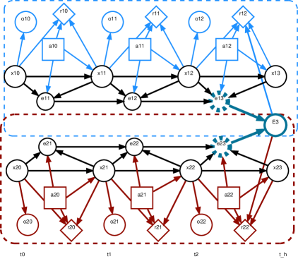
Figure 12: Local-form representation of TI-Dec-MDP: the LFMs of both agents (indicated by different color bounding boxes) are tied together by a influence source $E$ that indicates if the joint event happened. To be able to predict the value of this influence source, the agent $i$ will need to condition on their $e_{i}$ variable.

This class of problems includes, for instance, missions executed by Mars rovers during which they need to collect samples at various sites. In such settings, it is reasonable to assume that the rovers have their own routes and therefore will not affect each other’s transitions. However, the utility of rover 1 taking a soil sample at a particular site might depend on what samples are taken by rover 2 at nearby sites.

For instance, imagine that the rovers pass at different sides of a canyon, taking a picture of this canyon provides some utility, but if both rovers take a picture from their side of the canyon (corresponding to the individual events $e_{i}$), this may enable a better 3D reconstruction, providing more value than just the sum of two individual pictures.

This can be easily captured in a factored representation as shown in Figure 12. It shows that the combined occurrence of both agents’ events (as represented by Boolean variable $E$) leads to a change in the reward (split between the agents as soon as the event occurs). When the discount factor is 1 (as ? assume), the reward may as well be affected at the last time step as we have indicated. This leads to a very simple form of influence ${I}_{\rightarrow i}(e_{j}^{h-1})$ corresponding to the probability of $e_{j}^{h-1}$ being true. This corresponds exactly to the characterization of ‘parameter space’ presented by Becker et al. in their development of the coverage set algorithm (CSA).

Our characterization of the TI-Dec-MDP immediately leads to some new insights.

Observation.

While the TI-Dec-MDP framework is arguably more restrictive than the TD-POMDP, the graphical structure in Figure 12 makes clear that a TI-Dec-MDP is not a TD-POMDP: $E^{3}$ is affected from both sub-problems simultaneously.

Observation.

The properties that 1) events cannot occur more than once; and 2) events are unobserved, allow for history-independent influence encoding in TI-Dec-MDPs.

Observation.

CSA and closely-related TI-Dec-MDP algorithms (?) exploit structure that is also present in more general contexts, such as TI-Dec-POMDPs with partial observability of private factors.

That is, we make the observation that that CSA and its successors can actually be extended to more general problem whose joint value function is piecewise linear and convex in the influence parameters, such as settings where agents receive only partial observations of their local states.

7.3 Event-Driven Interactions

The TI-Dec-MDPs assumes that transitions are independent, but interactions are present in rewards. However, in many problems it may be the other way around: for instance, the rewards that a vacuum cleaner robot generates only depends on the amount of dirt it cleans up, but it cannot enter a dirty room until a general purpose house-hold robot opens the door.

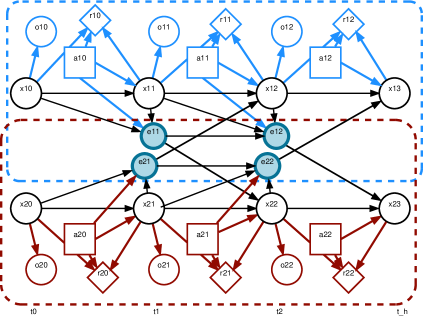
Figure 13: Local-form representation of the ED-Dec-MDP. The events $e_{1}$ act as influence destination for agent 2 and vice versa. To avoid clutter we do not indicate influence sources. The history of all $e_{i}$ serves as a d-separating set for both agents.

To deal with such problems ? (?) proposed the Dec-MDP with Event-Driven Interaction (EDI-Dec-MDP), which provides an explicit representation for structured transition dependencies between two agents. Again, we will interpret this model in the IBA framework, as illustrated in Figure 13. This figure shows that, agent $1$’s transition probabilities may be affected by the prior occurrence of agent 2’s event $e_{2}$ (and vice versa). In this case, the history of these event features are sufficient for d-separation, i.e., ${D}_{1}=\{e_{1},e_{2}\}$. This leads us to develop a new influence specification for this sub-class of problems:

Observation.

The (induced-CPT form of) influence on EDI-Dec-MDP agent $i$, ${I}_{\rightarrow i}^{t+1}({\pi}_{j})$ can be defined as $I({s}_{j}^{t},{a}_{j}^{t},{s}_{j}^{t+1}|\vec{e}_{i}^{\,t},\vec{e}_{j}^{\,t})$. Moreover, similar to what we saw in Section 4.4, the history $\vec{e}_{i}^{\,t},\vec{e}_{j}^{\,t}$ can be represented compactly since events can only switch to true.

The marginal of product of induced CPTs $Pr(e_{1}^{t+1},e_{2}^{t+1}|\vec{e}_{1}^{\,t},\vec{e}_{2}^{\,t})$ is similar to the parameters used by Becker et al. (in their application of CSA), but is slightly more compact, since it does not depend on private factors $s_{i}^{t}$, which our theory suggests to be unnecessary.

Having derived a more compact parameter form, we anticipate that this will translate directly into a more efficient application of CSA. We note that our reformulation of the TI-Dec-MDP and EDI-Dec-MDP also serve as influence specifications for the EDI-CR model (?), developed to include both event-driven interactions and reward dependencies (as in the TI-Dec-MDP).

The distributed POMDP with coordination locales (DPCL) model (?) can also be reinterpreted using Figure 13. This model assumes all agents’ observations are conditionally independent given the state, but that in some specific states, agents can affect each other’s transitions or rewards. Looking at Figure 13, the events $e_{i}$ precisely can model what ? refer to as future-time coordination locales (“situations where actions of one agent impact actions of others in the future”). ? also consider same-time coordination locales, which can model simultaneous effects such as robots failing to move when both try to move to the same grid cell. In Figure 13 this would be captured by adding arrows from $\vec{e}_{i}^{\,t}$ to ${s}_{i}^{t+1}$ (or alternatively by introducing joint events $E$, as in Figure 12, at every time step). While these same-time coordination locales overcome the modeling requirements of non-concurrency as observed in TD-POMDPs and ED-MDPs, the solution method proposed by ? is heuristic. In fact, it is precisely our definition of influence presented in this paper that explains how to deal with such concurrent interaction in a principled fashion.

7.4 ND-POMDP

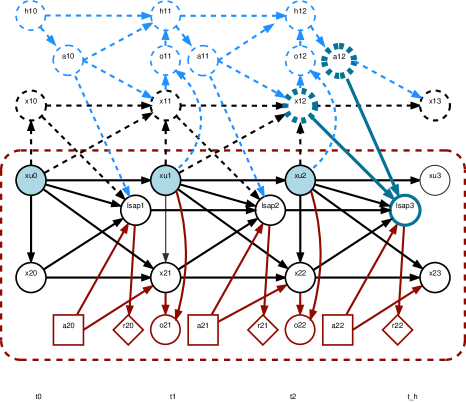
Figure 14: Local-form representation of agent 2 in a two-agent ND-POMDP. Highlighted are the influence sources for the “neighborhood state-action variable” ${z}^{3}$. (Time indices are omitted in the figure to avoid clutter, but can be inferred from the stages indicated at the bottom.) Note that because $z$ itself nor any of its descendants are observable (rewards are not observed in Dec-POMDPs), it does not open a path of influence to ${s}_{2}$. Therefore only the history of ${s}_{0}$ needs to be encoded in the d-separating set.

The Network Distributed POMDP (ND-POMDP) introduced by ? (?) is another transition and observation independent model whose structure can easily be represented in our framework. It was motivated by problems like sensor networks for intrusion detection, where the sensors need to select actions to scan their local surroundings. Such actions do not affect the local state of other sensors, but combinations of actions of neighboring sensor nodes can lead to higher rewards (e.g., if two adjacent sensors scan the same area where an intruder is, there might be a higher detection probability).

The formalization is depicted in Figure 14. Each agent’s observation can be affected by an unaffectable, mutually-modeled factor $s_{0}$ (e.g., the location of an intruder). The reward dependencies involving joint actions are captured with an unobservable variable $z$ encoding the local state-action pair that in much the same way as did the TI-Dec-MDP’s events. The difference is that these joint actions are not constrained to occur only once, and may affect the rewards at any time.

In general, an ND-POMDP can consist of multiple local neighborhoods, which can be modeled using a coordination (hyper-)graph (?, ?, ?). Agents correspond to nodes, while $\mathcal{E}$ is a set of (hyper-)edges corresponding to subsets, $e,$ of agents. To encode the interactions between different subsets of agents $e\in\mathcal{E}$, one can introduce different variables $z_{e}$. Our reformulation presented here immediately leads to the first specification of influence that we are aware of for this problem class. Let us write $N(i)$ to denote the neighbors of agent $i$ excluding agent $i$ itself: $N(i)=\left\{j\in\mathcal{D}|\exists e\in\mathcal{E}\;i,j\in e\;\wedge\;i\neq j\right\}$.

Observation.

The influence on ND-POMDP agent $i$, ${I}_{\rightarrow i}^{t+1}({\pi}_{-{i}})$ can be defined as

$${I}_{\rightarrow i}^{t+1}({s}_{N(i)}^{t},{a}_{N(i)}^{t}|\vec{s}_{0}^{~{}t})=\prod_{j\in N(i)}{I}_{j\rightarrow}^{t}({s}_{j}^{t},{a}_{j}^{t}|\vec{s}_{0}^{~{}t}),$$ (7.1)

with ${I}_{j\rightarrow}^{t}({s}_{j}^{t},{a}_{j}^{t}|\vec{s}_{0}^{~{}t})=\Pr({s}_{j}^{t},{a}_{j}^{t}|\vec{s}_{0}^{~{}t})$ the outgoing influence of agent $j$.

Like the other mentioned sub-classes, the ND-POMDP affords a compact influence encoding, suggesting that influence-based planning methods could gain traction if applied here. Existing forms of influence search exploit the fact that one can enumerate the joint influences, which describe how agents influence each other (?, ?). Due to the factorization of (7.1), the joint influence space here is a product space, which is easier to generate and search through. Moreover, it would be possible to exploit the graph structure of the ND-POMDP, similar to the approach by ? (?, Section 6.6): the space of joint influences can be decomposed as a factor graph over which one can optimize more effectively.

8 Related Work

Apart from the models and approaches reviewed in Section 7, there are important connections to be drawn with a large body of other work. Given the generality of the intuitive notion of ‘influence’ this should come as no surprise. Here we describe those relations to previous work and discuss further insights that our results provide. We sub-divide these related works in:

• work on locality of interaction and value factorization in multiagent systems,

• other decomposition-like approaches in multiagent systems, and

• more general forms of abstraction.

8.1 Locality of Interaction and Value Factorization

Past studies of factored Dec-POMDPs with factored value functions (?, ?, ?, ?) have shown that gains in computational efficiency are possible when the value function can be expressed as the sum of a number of local components, each of which is specified over subsets of agents and state factors. In particular, the value in general Dec-POMDPs can be expressed as a function $V_{\pi}({s}^{t},\vec{o}{}{}^{\,t})$ (e.g., see ?, chap. 3) of states and joint observation histories. Such a value function is said to be a factored value function if there is a set of components $e\in\mathcal{E}$ such that

$$V_{\pi}({s}^{t},\vec{o}{}{}^{\,t})=\sum_{e\in\mathcal{E}}V_{{\pi}_{e}}({s}_{e}^{t},{\vec{o}{}}_{e}^{\,t}),$$ (8.1)

with ${\pi}_{e}$ and ${\vec{o}{}}_{e}^{\,t}$ the policies respectively observation histories of the agents that participate in component $e$, and ${s}_{e}^{t}$ the value of the state factors relevant for $e$. For such problems, it is easy to show that they possess locality of interaction (?): one can define a local neighborhood for each agent such that its actions will not impact the value beyond that neighborhood. This property allows one to reduce the problem to a form of (distributed) constraint optimization problem (e.g., see ?, chap. 8) .

However, for general factored Dec-POMDPs, the components $e$ involve all agents and factors. I.e., they are not local (?, ?). This paper shows that even in the most general case, it actually is possible to find local (i.e., restricted scope) components, although this may be at the cost of introducing a dependence on the history of a subset of the local state factors (the d-separating set ${D}_{i}$). This means that it may be possible to extend the planning-as-inference method of (?) to exploit structure in general fDec-POMDPs. Researchers in the field of (deep) multiagent reinforcement learning, have tried to exploit such factorized structure approximately (?, ?, ?, ?, ?, ?, ?, ?, ?, ?), and our work brings deeper understanding of those approaches.

For instance, ? (?) proposed a form of factored value functions (?) making use of neural networks that can be understood better using the theory developed in this paper. Specifically they propose value-decomposition networks, a variant of deep Q-networks (DQN) introduced by ? (?), that uses a Q-function

$$\tilde{Q}(\vec{h},a)=\sum_{{i}\in\mathcal{D}}{\tilde{Q}}_{i}({\vec{h}}_{i},{a}_{i}),$$ (8.2)

which is implemented in a single neural network with a linear layer at the end that performs this summation. They state that

“the main assumption we make and exploit is that the joint action-value function for the system can be additively decomposed into value functions across agents”

and this assumption has been pointed out as a limitation in subsequent work (?, ?). This paper, however, demonstrates that there is a very large class of problems for which this assumption (approximately) holds. In particular, we show that for any factored Dec-POMDP for which we can create a set of local-form models (cf. Definition 10), we have that:

$$V_{\pi}(\vec{h})=\sum_{{i}\in\mathcal{D}}V_{i}({b}_{i}^{l})=\sum_{{i}\in\mathcal{D}}\max_{{a}_{i}}Q_{i}({b}_{i}^{l},{a}_{i}),$$ (8.3)

where ${b}_{i}^{l}$ is the local-form belief induced by ${\vec{h}}_{i}$ and the policies of the other agents ${\pi}_{-{i}}$. We also discuss that, by introducing dummy variables as required (cf. the end of Section 4.1.1), any factored Dec-POMDP can be re-coded as such set of local-from models. As such, there is a very large class of problems for which “the system can be additively decomposed into value functions across agents”. However, the devil is the details, we write “(approximately)” since the statement by ? (?) is about $Q$ not $V$. In particular, we have that

$$Q_{\pi}(\vec{h},a)\neq\sum_{{i}\in\mathcal{D}}Q_{i}({b}_{i}^{l},{a}_{i})$$ (8.4)

since each term $Q_{i}({b}_{i}^{l},{a}_{i})$ assumes that the other agents act according to ${\pi}_{-{i}}$, not according to $a$. This can explain the empirical improvements of methods that consider ‘higher order approximations’ with Q-components that involve subsets of agents (?, ?, ?).

We point out that this does not mean that an approximation $Q_{\pi}(\vec{h},a)\approx\sum_{{i}\in\mathcal{D}}Q_{i}({b}_{i}^{l},{a}_{i})$ is senseless: in fact, we know that for the modified joint policy $\pi^{\prime}$, which is like $\pi$ but does $a$ instead of $\pi(\vec{h})$, the decomposition of $V_{\pi^{\prime}}$ according to (8.3) also holds. As such, the question “how good of an approximation can we get with the individually factored Q-functions from (8.2)?” can be reinterpreted as a question of how the prediction of the components $Q_{i}({b}_{i}^{l},{a}_{i})$ (which assume the others follow ${\pi}_{-{i}}$) generalize to “first action modified policies” $\pi^{\prime}$. In other words, if for all such one-joint-action-modifications $\pi^{\prime}$ and their induced local form beliefs ${b}_{i}^{l\prime}$ we have that $Q_{i}({b}_{i}^{l},{a}_{i})\approx Q_{i}({b}_{i}^{l\prime},{a}_{i})$, then we expect this approximation to work well. Further formalizing the impact of such first-action-modifications may be a promising direction of research, and could lead to a novel notion of influence strength (?, ?) in multiagent domains.

We also remark that this analysis shows that, at least in cases that do not exhibit strict locality of interaction, value factorization inherently depends on the current policies of other agents, and hence implies an ‘on-policy characteristic’: when learning such factored value components we can only learn about the $Q_{i}({b}_{i}^{l},{a}_{i})$ that are induced by those ${\pi}_{-{i}}$ that are currently being followed by the other agents. Of course, agent $i$ itself can still try to learn its approximation ${\tilde{Q}}_{i}({\vec{h}}_{i},{a}_{i})$ with off-policy methods, but sudden large changes to the own policy may affect the ability of other agents to learn their local approximation. We speculate that in more tightly coupled problems on-policy methods with factorization may outperform off-policy ones.

8.2 More General Forms of Decomposition in MASs

In multiagent decision-making, there is a rich history of trying to leverage structured interactions. For instance, our approach resembles the distributed approximate planning method by ? (?) in that both methods decompose an agent’s decision model into internal and external parts. Our proposed abstraction, in addition to being sufficient for optimal decision-making, is more general in that it can deal with partial observability.

? (?, ?) proposed a different formalization of ‘influence’ by building upon information-theoretical concepts (mutual information between individual actions and joint states/observations/rewards). They show how their notion of influence and influence gap (which measures differences between the influencing power of agents) can predict the difficulty of solving a problem. While conceptually closely related to our work, their proposed notion of influence does not seem to support doing abstraction in any non-trivial manner, and thus should be seen as a very different type of object than our influence point.

The work by ? (?) is close in spirit to IBA: they propose to form a local abstraction of a factored MDP that approximates the original model well. Their approach is to abstract away a subset of exogenous variables (?) and they propose a method to select this subset. However, exogenous variables are defined as variables that can influence our local model, but that cannot be influenced by the local model. This stands in stark contrast to the non-modeled variables in IBA which can be affected by the local model.

Another class of related work is that focusing on anonymous interactions such as mean field games, D-SPAIT, and Collective Dec-POMDPs (?, ?, ?, ?, ?, ?). These models assume that the interactions between a large set of agents are governed by low dimensional statistics that capture how the rest of the population influences each individual. For instance, in disease propagation, only the number (not the identity) of people that are infected in one’s neighborhood might matter (?). As argued in the beginning of Section 5, the ability to include intra-stage connections into the IBA framework can enable us to model most (if not all) such problems in the IBA framework. So far, however, we have not yet identified how this can lead to compact influence representations (as described in Section 7) or more efficient approaches to solving these games.

? (?) investigate exploiting a heuristic form of influence in deterministic multiagent planning problems, formalized in the qualitative Dec-POMDP (?) framework. Their approach plans “per agent”: first each agent computes a plan assuming the other agents execute the actions that are most beneficial for it. This creates constraints (influences) for the other agents. Then the next agent gets to plan, subject to these constraints, and the process iterates.

In this work, we show how we can define a local-form model based upon a factored POSG model and a specification of a local state function $S$. We have not touched the question of how to define this local state function. E.g., in a multi-robot cleaning task, each agent potentially could clean every location, leading to local models as large as the original problem. To counter this, one can apply organizations (?, ?, ?) which effectively constrain which agents can address what parts of the problems. ? (?, ?) investigate such organizations in a decision-theoretic context, also taking into account simpler, approximate, forms of influence. Our definition of influence is different as it critically depends on the d-separating set, which is not considered by Sleight and Durfee. ? (?) use heuristics from multi-robot task allocation (?).

Other models (?, ?, ?, ?) have allowed for approximate decoupled local planning by leveraging a form of context-specific independence, where agents only influence each other in certain states. An important direction of research is to also exploit this type of independence in LFMs. Similar ideas have been considered in the multiagent RL setting too (?, ?). Structured interactions between agents are starting to be used for examining concepts like understanding by agents (?).

Approaches that take the perspective of a protagonist agent, like the recursive modeling method (?, ?), I-POMDPs (?), and work on ad-hoc teams (?, ?) inherently provide a subjective perspective, which can include modeling other agents recursively, that is conceptually related to our notion of the local model. Although the formal definition of these models is different from the fPOSG, our definition of influence (and thus IBA) is readily applicable to factored-state versions of these models, and therefore IBA can be extended to such models. Specifically, influence-based abstraction is conceptually similar to existing approaches that exploit behavioral equivalence (?, ?), but these approaches abstract classes of behaviors down to policies, whereas we abstract policies down to even more abstract influences. These relations are illustrated in Figure 15.

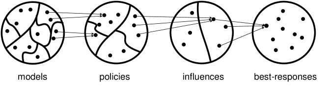
Figure 15: Many (e.g., I-POMDP) models for agent $j$ may be behaviorally equivalent, i.e., map to the same policy $\pi_{j}$. In turn, many policies ${\pi}_{j}$ can lead to the same influence ${I}_{\rightarrow i}$ on agent $i$. Finally, many influences may map to the same best-response ${\pi}_{i}$. (Note that only a small part of the space of ${\pi}_{i}$ may be a best-response to some influence/policy/model.)

Also in multiagent learning, the idea that abstract representations of influence exist and can help in learning are starting to be considered (?). For instance, ? (?) investigated an approximate form of influence of team mates in collaborative spatial task allocation problems. ? (?) propose ‘fingerprints’ (episode indices) for when data was collected to capture non-stationary due to the changing opponent strategy. ? (?) propose to augment DQN (?) with a module to learn ‘policy features’ based on observations of the actions of other agents. ? (?) propose to use a mutual information-based version of influence (similar to ?, discussed above) as an auxiliary reward, and ? (?) extended this to direct exploration in multiagent reinforcement learning. To some extent, all forms of agent modeling (e.g. ?, ?, ?) or tracking (?) can be seen as a some form of influence prediction, since one can think of the action of another agent as an influence source. However, few of these approaches further formalize the structure of this interaction, which means that they have not exploited the insight that one only may need to remember a subset of variables, even though this can lead to significant improvements (?).

8.3 Other Forms of Abstraction

Influence-based abstraction is a form of state abstraction, which has a long tradition in AI planning and learning (e.g., ?, ?, ?, ?, ?, ?, ?, ?, ?, ?, ?, ?, ?, ?, ?, ?) . Other types of abstraction (?) are temporal abstractions, such as options and macro-actions (?, ?, ?, ?), and functional abstraction, which tries to identify appropriate basis functions (?, ?, ?, ?), including the huge body of recent work on deep RL ç(?, ?, ?). We will focus on related work on state abstraction.

Different manners of performing state abstraction in MDPs exist, such as state aggregation methods which cluster similar states together, or starting with one abstract state and subsequently splitting (?), or removing state factors with no impact on the policy or rewards (?, ?). At a technical level these approaches are based on the idea that the original MDP and the abstraction are bisimilar. MDP homomorphisms (?, ?) generalize the idea of bisimilarity to also consider similarity of different actions. These ideas can also be used as metrics (?, ?), and many of these ideas lie at the core of recent model-based (deep) RL approaches (?, ?, ?, ?).

Other methods implement abstraction as part of the solution method (?, ?, ?). Different notions of which states to group together exist. ? (?) present a unifying framework that discriminates a number of types of exact state abstraction, and some of these were recently extended to approximate state abstractions (?). The introduced notions of model irrelevance/similarity are particularly relevant: they group together states that behave (approximately) identical in terms of rewards and transitions, which is also what IBA achieves in its influence-augmented local model.

However, there is one big difference between all these methods and the influence-based abstraction: in order to achieve a good approximation, all the previous notions can only group states together that have very similar (usually measured in L1 norm of) transition probabilities, which severely limits their applicability. Existing methods can generally not abstract away an entire state variable that is an influence source and still provide guarantees of near optimality. In contrast, IBA does enable abstracting away such influence sources, and thus groups together states that can have very different transition probabilities. IBA corrects for this by incorporating the influence in the IALM, by means of the dependence on the d-separating set ${D}_{i}$.

Another body of work casts abstracted, non-Markovian, models as models with imprecise probabilities (?, ?, ?, ?, ?, ?, ?). These typically place intervals on the transition probabilities and compute ‘robust’ policies that give the optimal worst case (with respect to the realized transition probabilities) payoff. Essentially these models are equivalent to a two-player zero-sum game where the agent faces an adversarial environment that chooses the transition probabilities to sabotage the agent (?). A disadvantage of such approaches is that they are only useful if the uncertainty intervals are sufficiently small and, as above, this is very hard to guarantee when abstracting away entire state variables. As such, the contribution of IBA is complimentary: it shows that it is possible to create abstract models which have no uncertainty interval at all.

IBA also bears some similarity to the framework of mixed-observability MDPs (?, ?), which splits the state $s=\left\langle o,l\right\rangle$ into observable state factors $o$ and hidden ones $l$. IBA, however, splits $s=\left\langle{x}_{i},{y}_{i}\right\rangle$ into modeled ${x}_{i}$ and non-modeled factors ${y}_{i}$. As such, the frameworks are complimentary: the local state space of an agent after performing IBA can have mixed observability and the hidden part $l$ of a mixed-observability MDPs can be abstracted by using IBA.

Finally, abstractions have also been investigated as the basis for robotic decision making (?) and multi-robot decision making (?, ?). These methods typically combine temporal and state abstraction. Specifically, ? (?) focus on learning abstract state representation that support open loop planning using a given set of ‘skills’ (also called ‘options’, ?, or ‘macro actions’, ?) and demonstrate this on a robot. While the formalization allows for probabilistic effects (they can reason about probability that the plan is executable), they assume that the skills are such that the effect of a skill $\sigma$ does not depend on the previous state, such that $\Pr(s^{\prime}|\sigma)$ is well defined. In practice, the approach typically requires small sets of states $s^{\prime}$ with positive support, or the probability of executability drops. As such, the framework is less suited for highly stochastic environments, such as those affected by other agents or other type of exogenous events (?). Thus, again, our work here is complementary, since it shows what parts of history may need to be retained to decrease this stochasticity. ? (?) focus on multi-robot motion planning. The difficulty here is to reason both about detailed motions, as well as the presence of multiple robots. To deal with this they propose to reason about the interaction (making use of multiagent path planning) in an abstract representation, this high-level plan is then used as a heuristic for the low-level motion planning. ? (?) formalize hierarchical Dec-POMDPs, called Mac-Dec-POMDP (for ‘macro-action’) where multiple agents act using options. The focus of this work lies on how to plan with options in the Dec-POMDP setting, but the abstractions at higher levels are assumed to be given.

9 Conclusion, Discussion and Future Work

This paper makes a theoretical contribution to the field of decision making in factored multiagent settings by giving a rigorous definition of influence-based abstraction (IBA) in such settings. It defines a notion of ‘influence’ that enables an agent in a POMDP to perform a lossless abstraction of the decision making problem it faces. That is, we prove that, for a given abstraction in terms of a local-form model, an influence point is a sufficient statistic for the part of the problem that is abstracted away. The local-form model and influence point together induce what we call an influence-augmented local model (IALM): a local model that is sufficient to compute an exact best response.

The proof of sufficiency also serves a practical purpose: it isolates the core technical property (in Section 6.2) that needs to hold for sufficiency. In this way it conveys insight into the nature of how abstraction of latent state factors affects value, provides a derivation that can be used to obtain simplifications of the definition of influence in simpler cases, and provides a recipe of how to prove similar results in more general cases.

At a higher level, IBA is important for the following reasons:

1. The theory presented in this paper presents a new perspective on abstraction in structured settings: it shows that such abstractions can be seen as special cases of POMDPs, where one only needs to remember about a subset of variables. Effectively, this can create a problem class in between MDPs and POMDPs: In this class, in order to predict the local dynamics, we will need to use memory, but this memory only needs to store information about the history of a subset of state variables.

2. It can enable more efficient best-response computation in fPOSGs, as well as providing a very natural form of approximation via approximate inference.

3. It provides a better understanding of previously identified sub-classes of fPOSGs (?, ?, ?, ?, ?, ?) and how they relate to each other. The insightful connections that we have drawn promote extensions of specialized methods beyond their respective sub-classes as well as comparisons with one another in more general contexts. For instance, our work has identified a compact representation of influences in ND-POMDPs (where none was known) and identified a more compact representation for EDI-Dec-MDPs.

4. It demonstrates how the value function for essentially any factored Dec-POMDP can be decomposed into the sum of a number of local value functions. As such, IBA demonstrates that all such problems satisfy a weak form of locality of interaction (also ‘value factorization’)—a property that is exploited in several Dec-POMDP solution methods (?, ?, ?) and multiagent RL papers (?, ?, ?, ?, ?, ?, ?, ?, ?, ?).

5. Influences can provide a more compact, yet sufficient statistic for the behavior of other agents in a MAS. We expect this to be important in multiagent reinforcement learning, since it is often easier to learn a compact statistic from the same amount of data.

We emphasize that this definition of influence is not a magic bullet: while the influence-augmented local model is sufficient to compute a best-response locally, the computation of the required influence point itself is an intractable inference problem in general. However, in certain cases where this problem is feasible it can enable faster best-response computations and search for multiagent plans via influence search (?, ?). As such, an important direction of future work would investigate how the definition of influence presented in this paper can support influence search in more general settings.

Moreover, even in cases where influences are intractable to compute, the concept forms the basis for principled approximations. For instance, by being optimistic with respect to the influence sources, one is able to compute upper bounds on the optimal value of Dec-POMDPs with hundreds of agents, thus leading to firm guarantees on the quality of heuristic solutions (?). Furthermore, there is evidence, in the context of deep reinforcement learning, that such approximate versions of influence may in some problems improve learning, both in terms of speed as well as performance (?). As such, a fruitful direction of research is to better understand such approximate characterization of influence (?). This article has provided the foundations for such an exploration.

An important direction of of future research would explore the applications of (approximate) forms of influence. For instance, it is possible that these can make a huge impact on human-robot interactions (?, ?). We note that even though the discussion in this paper was based on the more general case of multiagent systems, there is nothing that stops us from applying IBA in complex systems with just a single agent. As a case in point, ? (?) show improvements of learning on a single traffic intersection and on Atari games.

Finally, in this paper the discussion is limited to settings where structure is known. If we have structure, this can be exploited to define influence, possibly leading to more efficient best responses, or other benefits. Certainly, in many cases knowledge of the structure is not available. Future work could try to build off the advances in structure learning algorithms (?, ?, ?, ?) and their integration with decision making problems (?, ?, ?, ?, ?, ?); as long as it is possible to learn a model our methods would apply. In particular, even though such an estimated model might be inaccurate, its reduction to an IALM would add no further estimation error. This observation may open up a new research direction in sequential decision making that forsakes approximate solution methods (e.g., Monte Carlo tree search, ?, RL techniques like DQN, ?, or other forms of approximate dynamic programming, ?, ?, ?) in favor of learning useful approximate models that give structured representations of interactions. Arguably, such approaches that make exact use of assumed (but approximate) models lie at the basis of many, if not most, engineering disciplines and thus served human intelligence well in the past.

A Proofs and Derivations

Here we give proofs and derivations of a number of results. These are referred from the main text, and will be stated here without further explanation.

A.1 GFBRMs

A.1.1 Expected Reward

$$R_{i}({b}_{i}^{g},{a}_{i}^{t}) = \mathbf{E}_{{\bar{s}}_{i}^{t}\sim{b}_{i}^{g},{\bar{s}}_{i}^{t+1}\sim\bar{T}({\bar{s}}_{i}^{t},{a}_{i}^{t},\cdot)}\left[\bar{R_{i}}({\bar{s}}_{i}^{t},{a}_{i}^{t},{\bar{s}}_{i}^{t+1})\right]$$

$$= \sum_{{\bar{s}}_{i}^{t}}{b}_{i}^{g}({\bar{s}}_{i}^{t})\sum_{{\bar{s}}_{i}^{t+1}}\bar{T}({\bar{s}}_{i}^{t+1}|{\bar{s}}_{i}^{t},{a}_{i}^{t})\bar{R_{i}}({\bar{s}}_{i}^{t},{a}_{i}^{t},{\bar{s}}_{i}^{t+1})$$

$$= \sum_{\langle{s}^{t},{\vec{h}}_{-{i}}^{t}\rangle}{b}_{i}^{g}(\langle{s}^{t},{\vec{h}}_{-{i}}^{t}\rangle)\sum_{\langle{s}^{t+1},{\vec{h}}_{-{i}}^{t+1}\rangle}\Pr(\langle{s}^{t+1},{\vec{h}}_{-{i}}^{t+1}\rangle|\langle{s}^{t},{\vec{h}}_{-{i}}^{t}\rangle,{a}_{i})\bar{R_{i}}(\langle{s}^{t},{\vec{h}}_{-{i}}^{t}\rangle,{a}_{i},\langle{s}^{t+1},{\vec{h}}_{-{i}}^{t+1}\rangle)$$

$$= \sum_{\langle{s}^{t},{\vec{h}}_{-{i}}^{t}\rangle}{b}_{i}^{g}(\langle{s}^{t},{\vec{h}}_{-{i}}^{t}\rangle)\sum_{{s}^{t+1}}\sum_{{a}_{-{i}}}\sum_{{o}_{-{i}}^{t+1}}\Pr({s}^{t+1},{a}_{-{i}},{o}_{-{i}}^{t+1}|\langle{s}^{t},{\vec{h}}_{-{i}}^{t}\rangle,{a}_{i})R_{i}({s}^{t},{a}_{i},{a}_{-{i}},{s}^{t+1})$$

$$= \sum_{\langle{s}^{t},{\vec{h}}_{-{i}}^{t}\rangle}{b}_{i}^{g}(\langle{s}^{t},{\vec{h}}_{-{i}}^{t}\rangle)\sum_{{s}^{t+1}}\sum_{{a}_{-{i}}}\Pr({s}^{t+1},{a}_{-{i}}|\langle{s}^{t},{\vec{h}}_{-{i}}^{t}\rangle,{a}_{i})R_{i}({s}^{t},{a}_{i},{a}_{-{i}},{s}^{t+1})$$

$$= \sum_{{s}^{t}}\sum_{{s}^{t+1}}\sum_{{a}_{-{i}}}\Pr({s}^{t+1}|{s}^{t},a)R_{i}({s}^{t},a,{s}^{t+1})\sum_{{\vec{h}}_{-{i}}^{t}}\Pr({a}_{-{i}}|{\vec{h}}_{-{i}}^{t}){b}_{i}^{g}({s}^{t},{\vec{h}}_{-{i}}^{t})$$

A.1.2 Expected Observation Probability

$\Pr({o}_{i}^{t+1}|{b}_{i}^{g},{a}_{i}^{t})$

$$= \mathbf{E}_{{\bar{s}}_{i}^{t}\sim{b}_{i}^{g},{\bar{s}}_{i}^{t+1}\sim\bar{T}({\bar{s}}_{i}^{t},{a}_{i}^{t},\cdot)}\left[\bar{O}({o}_{i}^{t+1}|{a}_{i}^{t},{\bar{s}}_{i}^{t+1})\right]$$ (A.1)

$$= \sum_{{\bar{s}}_{i}^{t}}{b}_{i}^{g}({\bar{s}}_{i}^{t})\sum_{{\bar{s}}_{i}^{t+1}}\bar{T}({\bar{s}}_{i}^{t+1}|{\bar{s}}_{i}^{t},{a}_{i}^{t})\bar{O}({o}_{i}^{t+1}|{a}_{i}^{t},{\bar{s}}_{i}^{t+1})$$

$$= \sum_{\langle{s}^{t},{\vec{h}}_{-{i}}^{t}\rangle}{b}_{i}^{g}(\langle{s}^{t},{\vec{h}}_{-{i}}^{t}\rangle)\sum_{\langle{s}^{t+1},{\vec{h}}_{-{i}}^{t+1}\rangle}\Pr(\langle{s}^{t+1},{\vec{h}}_{-{i}}^{t+1}\rangle|\langle{s}^{t},{\vec{h}}_{-{i}}^{t}\rangle,{a}_{i})\Pr({o}_{i}|{a}_{i},\langle{s}^{t+1},{\vec{h}}_{-{i}}^{t+1}\rangle)$$

$$= \sum_{\langle{s}^{t},{\vec{h}}_{-{i}}^{t}\rangle}{b}_{i}^{g}(\langle{s}^{t},{\vec{h}}_{-{i}}^{t}\rangle)\sum_{{s}^{t+1}}\sum_{{a}_{-{i}}}\sum_{{o}_{-{i}}^{t+1}}\Pr({s}^{t+1},{a}_{-{i}},{o}_{-{i}}^{t+1}|\langle{s}^{t},{\vec{h}}_{-{i}}^{t}\rangle,{a}_{i})\Pr({o}_{i}|{a}_{i},{a}_{-{i}},{s}^{t+1},{o}_{-{i}}^{t+1})$$

$$= \sum_{\langle{s}^{t},{\vec{h}}_{-{i}}^{t}\rangle}{b}_{i}^{g}(\langle{s}^{t},{\vec{h}}_{-{i}}^{t}\rangle)\sum_{{s}^{t+1}}\sum_{{a}_{-{i}}}\sum_{{o}_{-{i}}^{t+1}}\Pr({s}^{t+1}|{s}^{t},{a}_{-{i}},{a}_{i})\Pr({a}_{-{i}}|{\vec{h}}_{-{i}}^{t},{\pi}_{-{i}})\Pr({o}_{-{i}}^{t+1}|{a}_{i},{a}_{-{i}},{s}^{t+1})$$

$$\quad\Pr({o}_{i}|{a}_{i},{a}_{-{i}},{s}^{t+1},{o}_{-{i}}^{t+1})$$

$$= \sum_{\langle{s}^{t},{\vec{h}}_{-{i}}^{t}\rangle}{b}_{i}^{g}(\langle{s}^{t},{\vec{h}}_{-{i}}^{t}\rangle)\sum_{{s}^{t+1}}\sum_{{a}_{-{i}}}\sum_{{o}_{-{i}}^{t+1}}\Pr({s}^{t+1}|{s}^{t},{a}_{-{i}},{a}_{i})\Pr({a}_{-{i}}|{\vec{h}}_{-{i}}^{t},{\pi}_{-{i}})\Pr({o}_{-{i}}^{t+1}|{a}_{i},{a}_{-{i}},{s}^{t+1})$$ (A.2)

$$\quad\frac{\Pr({o}_{i},{o}_{-{i}}^{t+1}|{a}_{i},{a}_{-{i}},{s}^{t+1})}{\Pr({o}_{-{i}}^{t+1}|{a}_{i},{a}_{-{i}},{s}^{t+1})}$$

$$= \sum_{\langle{s}^{t},{\vec{h}}_{-{i}}^{t}\rangle}{b}_{i}^{g}(\langle{s}^{t},{\vec{h}}_{-{i}}^{t}\rangle)\sum_{{s}^{t+1}}\sum_{{a}_{-{i}}}\sum_{{o}_{-{i}}^{t+1}}\Pr({s}^{t+1}|{s}^{t},a)\Pr({a}_{-{i}}|{\vec{h}}_{-{i}}^{t},{\pi}_{-{i}})\Pr({o}_{i},{o}_{-{i}}^{t+1}|{a}_{i},{a}_{-{i}},{s}^{t+1})$$

$$= \sum_{{s}^{t}}\sum_{{s}^{t+1}}\sum_{{a}_{-{i}}}\sum_{{o}_{-{i}}^{t+1}}\Pr({s}^{t+1}|{s}^{t},a)\Pr({o}^{t+1}|a,{s}^{t+1})\sum_{{\vec{h}}_{-{i}}^{t}}\Pr({a}_{-{i}}|{\vec{h}}_{-{i}}^{t},{\pi}_{-{i}}){b}_{i}^{g}({s}^{t},{\vec{h}}_{-{i}}^{t})$$

A.2 LFMs

A.2.1 Expected Reward

Starting with (3.5), we have that $R_{i}({b}_{i}^{g},{a}_{i})$

$$= \sum_{{s}^{t}}\sum_{{s}^{t+1}}\sum_{{a}_{-{i}}}\Pr({s}^{t+1}|{s}^{t},a)R_{i}({s}^{t},a,{s}^{t+1})\sum_{{\vec{h}}_{-{i}}^{t}}\Pr({a}_{-{i}}|{\vec{h}}_{-{i}}^{t},{\pi}_{-{i}}){b}_{i}^{g}({s}^{t},{\vec{h}}_{-{i}}^{t})$$

$$= \sum_{{s}^{t}}\sum_{{s}^{t+1}}\sum_{{a}_{-{i}}}\Pr({s}^{t+1}|{s}^{t},{a}_{i},{a}_{-{i}})R_{i}({s}^{t},a,{s}^{t+1})\sum_{{\vec{h}}_{-{i}}^{t}}\Pr({a}_{-{i}}|{\vec{h}}_{-{i}}^{t},{\pi}_{-{i}}){b}_{i}^{g}({s}^{t},{\vec{h}}_{-{i}}^{t})$$

$$= R_{i}$$ {restrict to actual dependencies of }

$$\sum_{{s}^{t}}\sum_{{s}^{t+1}}\sum_{{a}_{-{i}}}\Pr({s}^{t+1}|{s}^{t},{a}_{i},{a}_{-{i}})R_{i}({x}_{i}^{t},{a}_{i},{x}_{i}^{t+1})\sum_{{\vec{h}}_{-{i}}^{t}}\Pr({a}_{-{i}}|{\vec{h}}_{-{i}}^{t},{\pi}_{-{i}}){b}_{i}^{g}({s}^{t},{\vec{h}}_{-{i}}^{t})$$

$$= \sum_{{s}^{t}}\sum_{{a}_{-{i}}}\sum_{{x}_{i}^{t+1},{y}_{i}^{t+1}}\Pr({x}_{i}^{t+1},{y}_{i}^{t+1}|{s}^{t},{a}_{i},{a}_{-{i}})R_{i}({x}_{i}^{t},{a}_{i},{x}_{i}^{t+1})\sum_{{\vec{h}}_{-{i}}^{t}}\Pr({a}_{-{i}}|{\vec{h}}_{-{i}}^{t},{\pi}_{-{i}}){b}_{i}^{g}({s}^{t},{\vec{h}}_{-{i}}^{t})$$

$$=$$ {via (3.9)} (A.3)

$$\sum_{{x}_{i}^{t},{y}_{i}^{t}}\sum_{{a}_{-{i}}}\sum_{{x}_{i}^{t+1}}\Pr({x}_{i}^{t+1}|{s}^{t},{a}_{i},{a}_{-{i}})R_{i}({x}_{i}^{t},{a}_{i},{x}_{i}^{t+1})\sum_{{\vec{h}}_{-{i}}^{t}}\Pr({a}_{-{i}}|{\vec{h}}_{-{i}}^{t},{\pi}_{-{i}}){b}_{i}^{g}({s}^{t},{\vec{h}}_{-{i}}^{t})$$

$$= \sum_{{x}_{i}^{t}}\sum_{{x}_{i}^{t+1}}R_{i}({x}_{i}^{t},{a}_{i},{x}_{i}^{t+1})\sum_{{y}_{i}^{t}}\sum_{{a}_{-{i}}}\Pr({x}_{i}^{t+1}|{s}^{t},{a}_{i},{a}_{-{i}})\sum_{{\vec{h}}_{-{i}}^{t}}\Pr({a}_{-{i}}|{\vec{h}}_{-{i}}^{t},{\pi}_{-{i}}){b}_{i}^{g}({s}^{t},{\vec{h}}_{-{i}}^{t})$$

$$= \sum_{{x}_{i}^{t}}\sum_{{x}_{i}^{t+1}}R_{i}({x}_{i}^{t},{a}_{i},{x}_{i}^{t+1})\Pr({x}_{i}^{t},{x}_{i}^{t+1}|{b}_{i}^{g},{a}_{i}^{t},{\pi}_{-{i}}),$$

where we implicitly defined (remember ${s}^{t}=\langle{x}_{i}^{t},{y}_{i}^{t}\rangle$)

$$\Pr({x}_{i}^{t},{x}_{i}^{t+1}|{b}_{i}^{g},{a}_{i}^{t},{\pi}_{-{i}})\operatorname{\triangleq}\sum_{{y}_{i}^{t}}\sum_{{a}_{-{i}}}\Pr({x}_{i}^{t+1}|{s}^{t},{a}_{i},{a}_{-{i}})\sum_{{\vec{h}}_{-{i}}^{t}}\Pr({a}_{-{i}}|{\vec{h}}_{-{i}}^{t},{\pi}_{-{i}}){b}_{i}^{g}({s}^{t},{\vec{h}}_{-{i}}^{t})$$ (A.4)

A.2.2 Expected Observation Probability

In this case, the expected observation probability $\Pr({o}_{i}^{t+1}|{b}_{i}^{g},{a}_{i})$ equals

$$= \sum_{{s}^{t}}\sum_{{s}^{t+1}}\sum_{{a}_{-{i}}}\sum_{{o}_{-{i}}^{t+1}}\Pr({s}^{t+1}|{s}^{t},a)\Pr({o}^{t}|a,{s}^{t+1})\sum_{{\vec{h}}_{-{i}}^{t}}\Pr({a}_{-{i}}|{\vec{h}}_{-{i}}^{t},{\pi}_{-{i}}){b}_{i}^{g}({s}^{t},{\vec{h}}_{-{i}}^{t})$$ (A.5)

$$= \sum_{{s}^{t+1}}\sum_{{s}^{t}}\sum_{{a}_{-{i}}}\sum_{{o}_{-{i}}^{t+1}}\Pr({o}_{i}^{t+1},{o}_{-{i}}^{t+1}|{a}_{i},{a}_{-{i}},{s}^{t+1})\Pr({s}^{t+1}|{s}^{t},{a}_{i},{a}_{-{i}})$$

$$\sum_{{\vec{h}}_{-{i}}^{t}}\Pr({a}_{-{i}}|{\vec{h}}_{-{i}}^{t},{\pi}_{-{i}}){b}_{i}^{g}({s}^{t},{\vec{h}}_{-{i}}^{t})$$

$$=$$ {marginalize}

$$\sum_{{s}^{t+1}}\sum_{{s}^{t}}\sum_{{a}_{-{i}}}\Pr({o}_{i}^{t+1}|{a}_{i},{a}_{-{i}},{s}^{t+1})\Pr({s}^{t+1}|{s}^{t},{a}_{i},{a}_{-{i}})\sum_{{\vec{h}}_{-{i}}^{t}}\Pr({a}_{-{i}}|{\vec{h}}_{-{i}}^{t},{\pi}_{-{i}}){b}_{i}^{g}({s}^{t},{\vec{h}}_{-{i}}^{t})$$

$$=$$ {restrict to actual dependencies}

$$\sum_{{s}^{t+1}}\sum_{{s}^{t}}\sum_{{a}_{-{i}}}\Pr({o}_{i}^{t+1}|{a}_{i},{x}_{i}^{t+1})\Pr({s}^{t+1}|{s}^{t},{a}_{i},{a}_{-{i}})\sum_{{\vec{h}}_{-{i}}^{t}}\Pr({a}_{-{i}}|{\vec{h}}_{-{i}}^{t},{\pi}_{-{i}}){b}_{i}^{g}({s}^{t},{\vec{h}}_{-{i}}^{t})$$

$$= \sum_{{x}_{i}^{t+1},{y}_{i}^{t+1}}\sum_{{s}^{t}}\sum_{{a}_{-{i}}}\Pr({o}_{i}^{t+1}|{a}_{i},{x}_{i}^{t+1})\Pr({x}_{i}^{t+1},{y}_{i}^{t+1}|{s}^{t},{a}_{i},{a}_{-{i}})\sum_{{\vec{h}}_{-{i}}^{t}}\Pr({a}_{-{i}}|{\vec{h}}_{-{i}}^{t},{\pi}_{-{i}}){b}_{i}^{g}({s}^{t},{\vec{h}}_{-{i}}^{t})$$

$$= \sum_{{x}_{i}^{t+1}}\Pr({o}_{i}^{t+1}|{a}_{i},{x}_{i}^{t+1})\sum_{{s}^{t}}\sum_{{y}_{i}^{t+1}}\sum_{{a}_{-{i}}}\Pr({x}_{i}^{t+1},{y}_{i}^{t+1}|{s}^{t},{a}_{i},{a}_{-{i}})\sum_{{\vec{h}}_{-{i}}^{t}}\Pr({a}_{-{i}}|{\vec{h}}_{-{i}}^{t},{\pi}_{-{i}}){b}_{i}^{g}({s}^{t},{\vec{h}}_{-{i}}^{t})$$

$$= \sum_{{x}_{i}^{t+1}}\Pr({o}_{i}^{t+1}|{a}_{i},{x}_{i}^{t+1})\Pr({x}_{i}^{t+1}|{b}_{i}^{g},{a}_{i},{\pi}_{-{i}})$$

where we implicitly defined

$$\Pr({x}_{i}^{t+1}|{b}_{i}^{g},{a}_{i})\operatorname{\triangleq}\sum_{{s}^{t}}\sum_{{a}_{-{i}}}\Pr({x}_{i}^{t+1}|{s}^{t},{a}_{i},{a}_{-{i}})\sum_{{\vec{h}}_{-{i}}^{t}}\Pr({a}_{-{i}}|{\vec{h}}_{-{i}}^{t}{\pi}_{-{i}}){b}_{i}^{g}({s}^{t},{\vec{h}}_{-{i}}^{t}).$$ (A.6)

A.3 IALMs

A.3.1 Expected Observation Probability

$$\Pr({o}_{i}^{t+1}|{b}_{i}^{l},{a}_{i}^{t}) =\mathbf{E}_{{\bar{s}}_{i}^{t}\sim{b}_{i}^{l},{\bar{s}}_{i}^{t+1}\sim\bar{T}({\bar{s}}_{i}^{t},{a}_{i}^{t},\cdot)}\left[\bar{O}({o}_{i}^{t+1}|{a}_{i}^{t},{\bar{s}}_{i}^{t+1})\right]$$

$$=\sum_{{\bar{s}}_{i}^{t}}{b}_{i}^{l}({\bar{s}}_{i}^{t})\sum_{{\bar{s}}_{i}^{t+1}}\bar{T}({\bar{s}}_{i}^{t+1}|{\bar{s}}_{i}^{t},{a}_{i}^{t})\bar{O}({o}_{i}^{t+1}|{a}_{i}^{t},{\bar{s}}_{i}^{t+1})$$

$$= \sum_{{x}_{i}^{t},{D}_{i}^{t+1}}{b}_{i}^{l}({x}_{i}^{t},{D}_{i}^{t+1})\sum_{{x}_{i}^{t+1},{D}_{i}^{t+2}}\Pr({x}_{i}^{t+1},{D}_{i}^{t+2}|{x}_{i}^{t},{D}_{i}^{t+1},{a}_{i}^{t},{I}_{\rightarrow i}^{t+1})\Pr({o}_{i}^{t+1}|{a}_{i}^{t},{x}_{i}^{t+1})$$ (A.7)

$$= \sum_{{x}_{i}^{t},{D}_{i}^{t+1}}{b}_{i}^{l}({x}_{i}^{t},{D}_{i}^{t+1})\sum_{{x}_{i}^{t+1}}\Pr({x}_{i}^{t+1}|{x}_{i}^{t},{D}_{i}^{t+1},{a}_{i}^{t},{I}_{\rightarrow i}^{t+1})\Pr({o}_{i}^{t+1}|{a}_{i}^{t},{x}_{i}^{t+1})$$

$$= \sum_{{x}_{i}^{t+1}}\Pr({o}_{i}^{t+1}|{a}_{i}^{t},{x}_{i}^{t+1})\left[\sum_{{x}_{i}^{t},{D}_{i}^{t+1}}\Pr({x}_{i}^{t+1}|{x}_{i}^{t},{D}_{i}^{t+1},{a}_{i}^{t},{I}_{\rightarrow i}^{t+1}){b}_{i}^{l}({x}_{i}^{t},{D}_{i}^{t+1})\right]$$

$$= \sum_{{x}_{i}^{t+1}}\Pr({o}_{i}^{t+1}|{a}_{i}^{t},{x}_{i}^{t+1})\Pr({x}_{i}^{t+1}|{b}_{i}^{l},{a}_{i}^{t},{I}_{\rightarrow i}^{t+1}),$$

where we implicitly defined

$$\Pr({x}_{i}^{t+1}|{b}_{i}^{l},{a}_{i},{I}_{\rightarrow i}^{t+1})\operatorname{\triangleq}\sum_{{x}_{i}^{t},{D}_{i}^{t+1}}\Pr({x}_{i}^{t+1}|{x}_{i}^{t},{D}_{i}^{t+1},{a}_{i}^{t},{I}_{\rightarrow i}^{t+1}){b}_{i}^{l}({x}_{i}^{t},{D}_{i}^{t+1}).$$ (A.8)

(consistent with equation 4.12).

A.3.2 Expected Reward

$${R}_{i}({b}_{i}^{l},{a}_{i}^{t}) = \mathbf{E}_{{\bar{s}}_{i}^{t}\sim{b}_{i}^{l},{\bar{s}}_{i}^{t+1}\sim\bar{T}({\bar{s}}_{i}^{t},{a}_{i}^{t},\cdot)}\left[\bar{R_{i}}({\bar{s}}_{i}^{t},{a}_{i}^{t},{\bar{s}}_{i}^{t+1})\right]$$

$$= \sum_{{\bar{s}}_{i}^{t}}{b}_{i}^{l}({\bar{s}}_{i}^{t})\sum_{{\bar{s}}_{i}^{t+1}}\bar{T}({\bar{s}}_{i}^{t+1}|{\bar{s}}_{i}^{t},{a}_{i}^{t})\bar{R_{i}}({\bar{s}}_{i}^{t},{a}_{i}^{t},{\bar{s}}_{i}^{t+1})$$

$$= \sum_{{x}_{i}^{t},{D}_{i}^{t+1}}{b}_{i}^{l}({x}_{i}^{t},{D}_{i}^{t+1})\sum_{{x}_{i}^{t+1},{D}_{i}^{t+2}}\Pr({x}_{i}^{t+1},{D}_{i}^{t+2}|{x}_{i}^{t},{D}_{i}^{t+1},{a}_{i}^{t},{I}_{\rightarrow i}^{t+1}){R}_{i}({x}_{i}^{t},{a}_{i}^{t},{x}_{i}^{t+1})$$

$$= \sum_{{x}_{i}^{t},{D}_{i}^{t+1}}{b}_{i}^{l}({x}_{i}^{t},{D}_{i}^{t+1})\sum_{{x}_{i}^{t+1}}\Pr({x}_{i}^{t+1}|{x}_{i}^{t},{D}_{i}^{t+1},{a}_{i}^{t},{I}_{\rightarrow i}^{t+1}){R}_{i}({x}_{i}^{t},{a}_{i}^{t},{x}_{i}^{t+1})$$

$$= \sum_{{x}_{i}^{t}}\sum_{{x}_{i}^{t+1}}{R}_{i}({x}_{i}^{t},{a}_{i}^{t},{x}_{i}^{t+1})\left[\sum_{{D}_{i}^{t+1}}\Pr({x}_{i}^{t+1}|{x}_{i}^{t},{D}_{i}^{t+1},{a}_{i}^{t},{I}_{\rightarrow i}^{t+1}){b}_{i}^{l}({x}_{i}^{t},{D}_{i}^{t+1})\right]$$ (A.9)

$$= \sum_{{x}_{i}^{t}}\sum_{{x}_{i}^{t+1}}{R}_{i}({x}_{i}^{t},{a}_{i}^{t},{x}_{i}^{t+1})\Pr({x}_{i}^{t},{x}_{i}^{t+1}|{b}_{i}^{l},{a}_{i}^{t},{I}_{\rightarrow i}^{t+1})$$

where we implicitly defined

$$\Pr({x}_{i}^{t},{x}_{i}^{t+1}|{b}_{i}^{l},{a}_{i}^{t},{I}_{\rightarrow i}^{t+1})\operatorname{\triangleq}\sum_{{D}_{i}^{t+1}}\Pr({x}_{i}^{t+1}|{x}_{i}^{t},{D}_{i}^{t+1},{a}_{i}^{t},{I}_{\rightarrow i}^{t+1}){b}_{i}^{l}({x}_{i}^{t},{D}_{i}^{t+1})$$ (A.10)

(consistent with equation 4.16).

B List of Acronyms

Acronym	description
2DBN	2-stage dynamic Bayesian network
AOH	action-observation history
CPT	conditional probability table
DBN	dynamic Bayesian network
Dec-MDP	decentralized Markov decision process
Dec-POMDP	decentralized partially observable Markov decision process
EDI-Dec-MDP	Dec-MDP with event-driven interactions
fDec-POMDP	factored Dec-POMDP
fPOSG	factored POSG
GFBRMs	global-form best-response model
IALM	Influence-augmented local model
IBA	influence-based abstraction
ISDs	intra-stage dependencies
LFM	local-form model
MDP	Markov decision process
ND-POMDP	network-distributed POMDP
NLAF	non-locally affected factor
NMF	non-modeled factor
OLAF	only-locally affected factor
POMDP	partially observable Markov decision process
POSG	partially observable stochastic game
RL	reinforcement learning
TD-POMDP	transition-decoupled POMDP
TI-Dec-MDP	transition-independent Dec-MDP

C List of Notation

symbol	description
General
$\mathbf{E}\left[\cdot\right]$	expectation
$\Delta(\cdot)$	set of probability distributions over $\cdot$
$\boldsymbol{1}_{\{\cdot,\cdot\}}$	denotes the Kronecker delta function
${\left(\cdot\right)}_{i}$	a variable of interest $\left(\cdot\right)$ associated with agent $i$
${\left(\cdot\right)}_{-{i}}$	a tuple of variables associated with all agents except $i$
${\left(\cdot\right)}_{i}^{t}$	a variable of interest $\left(\cdot\right)$ associated with agent $i$ at time step $t$
${\left(\cdot\right)}^{k:t}$	partial history of values of $\left(\cdot\right)$ (e.g., $l_{tgt}^{k:t}$ is the history of target locations)
$\vec{\left(\cdot\right)}^{t}$	history of values of $\left(\cdot\right)$. I.e., $\vec{\left(\cdot\right)}^{t}={\left(\cdot\right)}^{0:t}$
Models
$\mathcal{M}^{POSG}$	A partially observable stochastic game (POSG)
$\mathcal{M}^{LFM}$	A local-form model: includes local state definitions for each agent
$\mathcal{M}_{i}^{GFBR}$	A global-form best-response model (GFBRM) for agent $i$
$\mathcal{M}_{i}^{IALM}$	An influence-augmented local model can be computed from an LFM when fixing other policies: $\mathcal{M}_{i}^{IALM}(\mathcal{M}^{LFM},{\pi}_{-{i}})$
Model components
$\mathcal{D}$	the set of agents or (d)ecision makers
$\mathcal{S}$	set of (global) states
$s$	a global (i.e., Markov) state
$\mathcal{A}$	set of (joint) actions $\mathcal{A}={\mathcal{A}}_{1}\times\dots\mathcal{A}_{n}$
$a$	a (joint) action $a=\left\langle{a}_{1},\dots,{a}_{n}\right\rangle$
$T$	transition function specifies $\Pr({s}^{t+1}|{s}^{t},{a}^{t})$
$\mathcal{R}$	set of reward functions
${R}_{i}$	reward function of agent $i$
$\mathcal{O}$	set of (joint) observations $\mathcal{O}={\mathcal{O}}_{1}\times\dots\times{\mathcal{O}}_{n}$
$o$	a (joint) observation $o=\left\langle{o}_{1},\dots,{o}_{n}\right\rangle$
$O$	observation function specifies $\Pr(o|a,s^{\prime})$
$\gamma$	the discount factor
$H$	horizon of the problem
${{b}}^{0}$	initial state distribution: ${{b}}^{0}\in\Delta(\mathcal{S})$
$\bar{{\mathcal{S}}_{i}}$	set of augmented states. E.g., in a GFBRM
$\bar{T}_{i},\bar{R}_{i}$,etc.	transitions, rewards, etc. over augmented states
histories and beliefs
${\vec{h}}_{i}^{t}$	the action-observation history (AOH) of agent $i$ at stage $t$
${\vec{\mathcal{H}}}_{i}^{t}$	the set of AOHs of agent $i$ at stage $t$
${{b}}$	belief of a single POMDP agent ${{b}}(s)\operatorname{\triangleq}\Pr(s|{{b}}^{0},{\vec{h}}^{t})$
$BU()$	The belief update ${{b}}^{\prime}=BU({{b}},{a},{o})$
${b}_{i}^{g}$	global-form belief of agent $i$
${b}_{i}^{l}$	local-form belief of agent $i$
${\pi}_{i}$	policy of agent $i$
Value functions
$V^{{t}}$	The optimal value function at stage $t$ with $H-t$ stages-to-go
${Q}^{t}$	The optimal action-value function, or ‘Q-function’
Factored States
$\mathcal{F}$	the set of state factors $\mathcal{F}=\left\{{F}^{1},\dots,{F}^{|\mathcal{F}|}\right\}$ in a factored model, we have that $\mathcal{S}={\mathcal{F}}^{1}\times\dots\times{\mathcal{F}}^{|\mathcal{F}|}$
${F}^{k}$	the $k$-th state factor
${\mathcal{F}}^{k}$	the set of values ${f}^{k}\in{\mathcal{F}}^{k}$ that ${F}^{k}$ can take
${f}^{k}$	a value of state factor $k$
$\text{ORel}{}_{i}(F)$	observation relevant factor of agent $i$
$\text{RRel}{}_{i}(F)$	reward relevant factor of agent $i$
Local states of agent $i$
${\mathcal{S}}_{i}$	state space of agent $i$ (general term: also outside LFMs)
${s}_{i}$	state for agent $i$ (general term: also outside LFMs)
$S(i)$	the local state function of an LFM for agent $i$: partitions $\mathcal{F}$ into modeled state factors ${x}^{k}$ and non-modeled ones ${y}^{k}$
${x}^{k}$	$k$-th modeled factor
${\mathring{x}}^{k}$	$k$-th only-locally-affected factor (OLAF): a modeled factor that is not an influence destination
${\tilde{x}}^{k}$	$k$-th a non-locally-affected factor (NLAF): a modeled factor that is an influence destination
${\mathcal{X}}_{i}$	local state space (of modeled factors) in an LFM
${x}_{i}$	local state of agent $i$ in an LFM
${y}^{k}$	a non-modeled factor
${y}_{i}$	instantiation of all non-modeled factors. I.e., $s=\left\langle{x}_{i},{y}_{i}\right\rangle$
$OLAF(i)$	the set of OLAFs
$NLAF(i)$	the set of NLAFs
Influence notation
${u}_{\rightarrow i}^{t}$	instantiation of all direct influence sources for stage $t$: ${u}_{\rightarrow i}^{t}=\langle{y}_{u}^{t-1},{a}_{u}^{t-1},{y}_{u}^{t}\rangle$
${y}_{u}^{t-1}$	the (non-modeled) state factors that are direct influence sources
${y}_{u}^{t}$	the (non-modeled) state factors that are direct intra-stage influence sources
${a}_{u}^{t-1}$	the actions (of some subset of agents) that are direct influence sources
$\vec{h}{}_{u}^{t-1}$	the AOHs of those other agents whose action is an influence source (i.e., $\vec{h}{}_{u}^{t-1}$ involves the same agents as ${a}_{u}^{t-1}$)
$v$	indirect sources: ${y}_{v}^{t-1}$, ${a}_{u}^{t-1}$, ${y}_{v}^{t}$ can effect the direct sources ${u}_{\rightarrow i}^{t}$
$w$	union of direct and indirect sources: $w=u\cup v$; e.g., ${\pi}_{w}$ is the joint policy of those agents whose action is either a direct or an indirect influence source
${D}_{i}^{t}$	a d-separating set for agent $i$’s influence at stage $t$
$d$	the d-set update function: ${D}_{i}^{t+2}=d({x}_{i}^{t},{a}_{i}^{t},{x}_{i}^{t+1},{D}_{i}^{t+1})$
$\sigma$	the d-set compression function $\sigma({D}_{i}^{t+1})$ that computes a sufficient statistic for ${D}_{i}^{t+1}$
${I}_{\rightarrow i}({\pi}_{-{i}})$	${I}_{\rightarrow i}({\pi}_{-{i}})=\left({I}_{\rightarrow i}^{1}({\pi}_{-{i}}),\dots,{I}_{\rightarrow i}^{H}({\pi}_{-{i}})\right)$ is an incoming influence point ${I}_{\rightarrow i}({\pi}_{-{i}})$
${I}_{\rightarrow i}^{t}({\pi}_{-{i}})$	The incoming influence at stage $t$: a conditional probability distribution over values of the influence sources
$I({u}_{\rightarrow i}^{t}|{D}_{i}^{t})$	shorthand for ${I}_{\rightarrow i}^{t}({u}_{\rightarrow i}^{t}|{D}_{i}^{t},{{b}}^{0},{\pi}_{-{i}})={I}_{\rightarrow i}^{t}({\pi}_{-{i}})({u}_{\rightarrow i}^{t}|{D}_{i}^{t},{{b}}^{0})$
$p_{{I}_{\rightarrow i}^{t+1}}$	influence-induced CPT that specifies $p_{{I}_{\rightarrow i}^{t+1}}({\tilde{x}}^{t+1}|{x}_{i}^{t},{D}_{i}^{t+1},{a}_{i})$

References

- Abel et al. Abel, D., Arumugam, D., Asadi, K., Jinnai, Y., Littman, M. L., and Wong, L. L. (2019). State abstraction as compression in apprenticeship learning. In Proc. of the Thirty-Third AAAI Conference on Artificial Intelligence, pp. 3134–3142.
- Abel et al. Abel, D., Hershkowitz, D. E., and Littman, M. L. (2016). Near optimal behavior via approximate state abstraction. In Proc. of the Thirty-Third International Conference on Machine learning, pp. 2915–2923.
- Acid and De Campos Acid, S., and De Campos, L. M. (1996). An algorithm for finding minimum d-separating sets in belief networks. In Proc. of the Twelfth Conference on Uncertainty in Artificial Intelligence, pp. 3–10.
- Albrecht and Ramamoorthy Albrecht, S., and Ramamoorthy, S. (2013). A game-theoretic model and best-response learning method for ad hoc coordination in multiagent systems. In Proc. of the Twelfth International Conference on Autonomous Agents and Multiagent Systems, pp. 1155–1156.
- Allen and Zilberstein Allen, M., and Zilberstein, S. (2007). Agent influence as a predictor of difficulty for decentralized problem-solving. In Proc. of the National Conference on Artificial Intelligence, pp. 688–693.
- Allen and Zilberstein Allen, M., and Zilberstein, S. (2009). Agent influence and intelligent approximation in multiagent problems. In Proc. of the International Conference on Intelligent Agent Technology, pp. 311–314.
- Amato et al. Amato, C., Konidaris, G., Kaelbling, L. P., and How, J. P. (2019). Modeling and planning with macro-actions in decentralized POMDPs. Journal of Artificial Intelligence Research, 64, 817–859.
- Anand et al. Anand, A., Noothigattu, R., Mausam, and Singla, P. (2016). OGA-UCT: on-the-go abstractions in UCT. In Proc. of the Twenty-Sixth International Conference on Automated Planning and Scheduling, pp. 29–37.
- Bai et al. Bai, A., Srivastava, S., and Russell, S. J. (2016). Markovian state and action abstractions for MDPs via hierarchical MCTS. In Proc. of the Twenty-Fifth International Joint Conference on Artificial Intelligence, pp. 3029–3039.
- Bazinin and Shani Bazinin, S., and Shani, G. (2018). Iterative planning for deterministic QDec-POMDPs. In Proc. of the 4th Global Conference on Artificial Intelligence, Vol. 55, pp. 15–28.
- Becker et al. Becker, R., Zilberstein, S., and Lesser, V. (2004). Decentralized Markov decision processes with event-driven interactions. In Proc. of the International Conference on Autonomous Agents and Multiagent Systems, pp. 302–309.
- Becker et al. Becker, R., Zilberstein, S., Lesser, V., and Goldman, C. V. (2003). Transition-independent decentralized Markov decision processes. In Proc. of the International Conference on Autonomous Agents and Multiagent Systems, pp. 41–48.
- Bertsekas Bertsekas, D. P. (2005). Dynamic Programming and Optimal Control (3rd edition)., Vol. I. Athena Scientific.
- Bertsekas Bertsekas, D. P. (2007). Dynamic Programming and Optimal Control (3rd edition)., Vol. II. Athena Scientific.
- Bishop Bishop, C. M. (2006). Pattern Recognition and Machine Learning. Springer.
- Biza and Platt Biza, O., and Platt, R. (2019). Online abstraction with MDP homomorphisms for deep learning. In Proc. of the Eighteenth International Conference on Autonomous Agents and Multiagent Systems, pp. 1125–1133.
- Böhmer et al. Böhmer, W., Kurin, V., and Whiteson, S. (2019). Deep coordination graphs. arXiv e-prints, arXiv:1910.00091.
- Boutilier et al. Boutilier, C., Dean, T., and Hanks, S. (1999). Decision-theoretic planning: Structural assumptions and computational leverage. Journal of Artificial Intelligence Research, 11, 1–94.
- Boutilier et al. Boutilier, C., Dearden, R., and Goldszmidt, M. (2000). Stochastic dynamic programming with factored representations. Artificial Intelligence, 121(1-2), 49–107.
- Boyen and Koller Boyen, X., and Koller, D. (1998). Tractable inference for complex stochastic processes. In Proc. of Uncertainty in Artificial Intelligence, pp. 33–42.
- Brafman et al. Brafman, R. I., Shani, G., and Zilberstein, S. (2013). Qualitative planning under partial observability in multi-agent domains. In Proc. of the Twenty-Seventh AAAI Conference on Artificial Intelligence, pp. 130–137.
- Browne et al. Browne, C., Powley, E. J., Whitehouse, D., Lucas, S. M., Cowling, P. I., Rohlfshagen, P., Tavener, S., Perez, D., Samothrakis, S., and Colton, S. (2012). A survey of Monte Carlo tree search methods. IEEE Trans. Comput. Intellig. and AI in Games, 4(1), 1–43.
- Carley and Gasser Carley, K. M., and Gasser, L. (1999). Computational organization theory. In Multiagent systems: A modern approach to distributed artificial intelligence, pp. 299–330. MIT Press.
- Castellini et al. Castellini, J., Oliehoek, F. A., Savani, R., and Whiteson, S. (2019). The representational capacity of action-value networks for multi-agent reinforcement learning. In Proc. of the Eighteenth International Conference on Autonomous Agents and Multiagent Systems, pp. 1862–1864.
- Chitnis and Lozano-Pérez Chitnis, R., and Lozano-Pérez, T. (2020). Learning compact models for planning with exogenous processes. In Proceedings of the Conference on Robot Learning, pp. 813–822.
- Cho et al. Cho, K., van Merriënboer, B., Gulcehre, C., Bahdanau, D., Bougares, F., Schwenk, H., and Bengio, Y. (2014). Learning phrase representations using RNN encoder–decoder for statistical machine translation. In Proc. of the 2014 Conference on Empirical Methods in Natural Language Processing, pp. 1724–1734.
- Claes et al. Claes, D., Oliehoek, F. A., Baier, H., and Tuyls, K. (2017). Decentralised online planning for multi-robot warehouse commisioning. In Proc. of the Sixteenth International Conference on Autonomous Agents and Multiagent Systems, pp. 492–500.
- Claes et al. Claes, D., Robbel, P., Oliehoek, F. A., Hennes, D., Tuyls, K., and Van der Hoek, W. (2015). Effective approximations for multi-robot coordination in spatially distributed tasks. In Proc. of the Fourteenth International Conference on Autonomous Agents and Multiagent Systems, pp. 881–890.
- Congeduti et al. Congeduti, E., Mey, A., and Oliehoek, F. A. (2020). Loss bounds for approximate influence-based abstraction. arXiv e-prints, arXiv:2011.01788.
- Corneil et al. Corneil, D., Gerstner, W., and Brea, J. (2018). Efficient model-based deep reinforcement learning with variational state tabulation. In Proc. of the 35th International Conference on Machine Learning, pp. 1049–1058.
- Corona et al. Corona, R., Alaniz, S., and Akata, Z. (2019). Modeling Conceptual Understanding in Image Reference Games. arXiv e-prints, arXiv:1910.04872.
- De Hauwere et al. De Hauwere, Y.-M., Vrancx, P., and Nowé, A. (2010). Learning multi-agent state space representations. In Proc. of the International Conference on Autonomous Agents and Multiagent Systems, pp. 715–722.
- Dean and Givan Dean, T., and Givan, R. (1997). Model minimization in Markov decision processes.. In Proc. of the National Conference on Artificial Intelligence, pp. 106–111.
- Dean et al. Dean, T., Givan, R., and Leach, S. M. (1997). Model reduction techniques for computing approximately optimal solutions for Markov decision processes.. In Proc. of Uncertainty in Artificial Intelligence, pp. 124–131.
- Dearden and Boutilier Dearden, R., and Boutilier, C. (1997). Abstraction and approximate decision-theoretic planning. Artificial Intelligence, 89(1-2), 219–283.
- Degris et al. Degris, T., Sigaud, O., and Wuillemin, P.-H. (2006). Learning the structure of factored Markov decision processes in reinforcement learning problems. In Proc. of the Twenty-Third International Conference on Machine learning, pp. 257–264.
- Delgado et al. Delgado, K. V., de Barros, L. N., Dias, D. B., and Sanner, S. (2016). Real-time dynamic programming for Markov decision processes with imprecise probabilities. Artificial Intelligence, 230, 192–223.
- Delgado et al. Delgado, K. V., de Barros, L. N., Cozman, F. G., and Sanner, S. (2011a). Using mathematical programming to solve factored Markov decision processes with imprecise probabilities. International Journal of Approximate Reasoning, 52(7), 1000–1017.
- Delgado et al. Delgado, K. V., Sanner, S., and de Barros, L. N. (2011b). Efficient solutions to factored MDPs with imprecise transition probabilities. Artificial Intelligence, 175(9-10), 1498–1527.
- Doshi-Velez Doshi-Velez, F. (2009). The infinite partially observable Markov decision process. In Advances in Neural Information Processing Systems 22, pp. 477–485.
- Doshi-Velez et al. Doshi-Velez, F., Wingate, D., Tenenbaum, J. B., and Roy, N. (2011). Infinite dynamic Bayesian networks. In Proc. of the Twenty-Eighth International Conference on Machine learning, pp. 913–920.
- Ferber et al. Ferber, J., Gutknecht, O., and Michel, F. (2004). From agents to organizations: An organizational view of multi-agent systems. In Proc. of the 4th International Workshop on Agent-Oriented Software Engineering, pp. 214–230.
- Ferns et al. Ferns, N., Panangaden, P., and Precup, D. (2004). Metrics for finite Markov decision processes. In Proc. of the Twentieth Conference on Uncertainty in Artificial Intelligence, pp. 162–169.
- Ferns and Precup Ferns, N., and Precup, D. (2014). Bisimulation metrics are optimal value functions. In Proc. of the Thirtieth Conference on Uncertainty in Artificial Intelligence, pp. 210–219.
- Foerster et al. Foerster, J. N., Nardelli, N., Farquhar, G., Afouras, T., Torr, P. H. S., Kohli, P., and Whiteson, S. (2017). Stabilising experience replay for deep multi-agent reinforcement learning. In Proc. of the Thirty-Fourth International Conference on Machine learning, pp. 1146–1155.
- François-Lavet et al. François-Lavet, V., Henderson, P., Islam, R., Bellemare, M. G., and Pineau, J. (2018). An introduction to deep reinforcement learning. Foundations and Trends in Machine Learning, 11(3-4), 219–354.
- Gelada et al. Gelada, C., Kumar, S., Buckman, J., Nachum, O., and Bellemare, M. G. (2019). DeepMDP: Learning continuous latent space models for representation learning. In Proc. of the Thirty-Sixth International Conference on Machine learning, Vol. 97, pp. 2170–2179.
- Gerkey and Mataric Gerkey, B. P., and Mataric, M. J. (2003). Multi-robot task allocation: Analyzing the complexity and optimality of key architectures. In Proc. of the International Conference on Robotics and Automation, pp. 3862–3868.
- Givan et al. Givan, R., Dean, T., and Greig, M. (2003). Equivalence notions and model minimization in Markov decision processes. Artificial Intelligence, 14(1–2), 163–223.
- Givan et al. Givan, R., Leach, S. M., and Dean, T. L. (2000). Bounded-parameter Markov decision processes. Artificial Intelligence, 122(1-2), 71–109.
- Gmytrasiewicz and Doshi Gmytrasiewicz, P. J., and Doshi, P. (2005). A framework for sequential planning in multi-agent settings. Journal of Artificial Intelligence Research, 24, 49–79.
- Gmytrasiewicz and Durfee Gmytrasiewicz, P. J., and Durfee, E. H. (1995). A rigorous, operational formalization of recursive modeling. In Proc. of the First International Conference on Multiagent Systems, pp. 125–132.
- Gmytrasiewicz and Durfee Gmytrasiewicz, P. J., and Durfee, E. H. (2000). Rational coordination in multi-agent environments. Journal of Autonomous Agents and Multi-Agent Systems, 3(4), 319–350.
- Graves et al. Graves, A., Mohamed, A.-r., and Hinton, G. (2013). Speech recognition with deep recurrent neural networks. In 2013 IEEE international conference on acoustics, speech and signal processing, pp. 6645–6649. IEEE.
- Guestrin and Gordon Guestrin, C., and Gordon, G. (2002). Distributed planning in hierarchical factored MDPs. In Proc. of Uncertainty in Artificial Intelligence, pp. 197–206.
- Guestrin et al. Guestrin, C., Koller, D., and Parr, R. (2002a). Multiagent planning with factored MDPs. In Advances in Neural Information Processing Systems 14, pp. 1523–1530.
- Guestrin et al. Guestrin, C., Lagoudakis, M., and Parr, R. (2002b). Coordinated reinforcement learning. In Proc. of the International Conference on Machine Learning, pp. 227–234.
- Hansen et al. Hansen, E. A., Bernstein, D. S., and Zilberstein, S. (2004). Dynamic programming for partially observable stochastic games. In Proc. of the National Conference on Artificial Intelligence, pp. 709–715.
- He et al. He, J., Suau, M., and Oliehoek, F. A. (2020). Influence-augmented online planning for complex environments. In Advances in Neural Information Processing Systems 33.
- Hernandez-Leal et al. Hernandez-Leal, P., Kaisers, M., Baarslag, T., and Munoz de Cote, E. (2017). A Survey of Learning in Multiagent Environments: Dealing with Non-Stationarity. arXiv e-prints, arXiv:1707.09183.
- Hernandez-Leal et al. Hernandez-Leal, P., Kartal, B., and Taylor, M. E. (2019). Agent modeling as auxiliary task for deep reinforcement learning. In Proc. of the AAAI Conference on Artificial Intelligence and Interactive Digital Entertainment, pp. 31–37.
- Hoey et al. Hoey, J., St-Aubin, R., Hu, A. J., and Boutilier, C. (1999). SPUDD: Stochastic planning using decision diagrams. In Proc. of Uncertainty in Artificial Intelligence, pp. 279–288.
- Hong et al. Hong, Z.-W., Su, S.-Y., Shann, T.-Y., Chang, Y.-H., and Lee, C.-Y. (2018). A deep policy inference Q-Network for multi-agent systems. In Proc. of the Seventeenth International Conference on Autonomous Agents and MultiAgent Systems, pp. 1388–1396.
- Hostetler et al. Hostetler, J., Fern, A., and Dietterich, T. (2014). State aggregation in monte carlo tree search. In Proc. of the Twenty-Eighth AAAI Conference on Artificial Intelligence, pp. 2446–2452.
- Howard and Matheson Howard, R. A., and Matheson, J. E. (1984). Influence diagrams. In The Principles and Applications of Decision Analysis, Vol. II., pp. 719–763. Strategic Decisions Group.
- Iyengar Iyengar, G. N. (2005). Robust dynamic programming. Mathematics of Operations Research, 30(2), 257–280.
- Jaques et al. Jaques, N., Lazaridou, A., Hughes, E., Gulcehre, C., Ortega, P., Strouse, D., Leibo, J. Z., and De Freitas, N. (2019). Social influence as intrinsic motivation for multi-agent deep reinforcement learning. In Proc. of the Thirty-Sixth International Conference on Machine learning, pp. 3040–3049.
- Jong and Stone Jong, N. K., and Stone, P. (2005). State abstraction discovery from irrelevant state variables. In Proc. of the Nineteenth International Joint Conference on Artificial Intelligence, pp. 752–757.
- Jordan et al. Jordan, M. I., Ghahramani, Z., Jaakkola, T. S., and Saul, L. K. (1999). An introduction to variational methods for graphical models. Machine learning, 37(2), 183–233.
- Jovanovic and Rosenthal Jovanovic, B., and Rosenthal, R. W. (1988). Anonymous sequential games. Journal of Mathematical Economics, 17(1), 77 – 87.
- Jurtz et al. Jurtz, V. I., Johansen, A. R., Nielsen, M., Almagro Armenteros, J. J., Nielsen, H., Sønderby, C. K., Winther, O., and Sønderby, S. K. (2017). An introduction to deep learning on biological sequence data: examples and solutions. Bioinformatics, 33(22), 3685–3690.
- Kaelbling et al. Kaelbling, L. P., Littman, M. L., and Cassandra, A. R. (1998). Planning and acting in partially observable stochastic domains. Artificial Intelligence, 101(1-2), 99–134.
- Kaelbling and Lozano-Perez Kaelbling, L. P., and Lozano-Perez, T. (2012). Integrated robot task and motion planning in the now. Tech. rep. TR-2012-018, MIT CSAIL.
- Katt et al. Katt, S., Oliehoek, F. A., and Amato, C. (2019). Bayesian reinforcement learning in factored POMDPs. In Proc. of the Eighteenth International Conference on Autonomous Agents and Multiagent Systems, pp. 7–15.
- Keller et al. Keller, P. W., Mannor, S., and Precup, D. (2006). Automatic basis function construction for approximate dynamic programming and reinforcement learning. In Proc. of the Twenty-Third International Conference on Machine learning, pp. 449–456.
- Kim et al. Kim, Y., Nair, R., Varakantham, P., Tambe, M., and Yokoo, M. (2006). Exploiting locality of interaction in networked distributed POMDPs. In Proc. of the AAAI Spring Symposium on Distributed Plan and Schedule Management.
- Kizilkale and Caines Kizilkale, A. C., and Caines, P. E. (2012). Mean field stochastic adaptive control. IEEE Transactions on Automatic Control, 58(4), 905–920.
- Knoblock Knoblock, C. A. (1993). Generating Abstraction Hierarchies: An Automated Approach to Reducing Search in Planning. Kluwer Academic Publishers.
- Kok and Vlassis Kok, J. R., and Vlassis, N. (2006). Collaborative multiagent reinforcement learning by payoff propagation. Journal of Machine Learning Research, 7, 1789–1828.
- Koller and Friedman Koller, D., and Friedman, N. (2009). Probabilistic Graphical Models: Principles and Techniques. MIT Press.
- Konidaris and Barto Konidaris, G., and Barto, A. G. (2009). Efficient skill learning using abstraction selection. In Proc. of the Twenty-First International Joint Conference on Artificial Intelligence, pp. 1107–1112.
- Konidaris et al. Konidaris, G., Kaelbling, L. P., and Lozano-Pérez, T. (2018). From skills to symbols: Learning symbolic representations for abstract high-level planning. Journal of Artificial Intelligence Research, 61, 215–289.
- Kumar et al. Kumar, A., Zilberstein, S., and Toussaint, M. (2011). Scalable multiagent planning using probabilistic inference. In Proc. of the International Joint Conference on Artificial Intelligence, pp. 2140–2146.
- Kuyer et al. Kuyer, L., Whiteson, S., Bakker, B., and Vlassis, N. (2008). Multiagent reinforcement learning for urban traffic control using coordination graphs. In Machine Learning and Knowledge Discovery in Databases, pp. 656–671.
- Lauri et al. Lauri, M., Pajarinen, J., and Peters, J. (2020). Multi-agent active information gathering in discrete and continuous-state decentralized pomdps by policy graph improvement. Journal of Autonomous Agents and Multi-Agent Systems, 34(42).
- Le and Plaku Le, D., and Plaku, E. (2018). Cooperative, dynamics-based, and abstraction-guided multi-robot motion planning. Journal of Artificial Intelligence Research, 63, 361–390.
- LeCun et al. LeCun, Y., Bengio, Y., and Hinton, G. (2015). Deep learning. Nature, 521(7553), 436–444.
- Li et al. Li, L., Walsh, T. J., and Littman, M. L. (2006). Towards a unified theory of state abstraction for MDPs. In International Symposium on Artificial Intelligence and Mathematics.
- Littman Littman, M. L. (1994). Memoryless policies: Theoretical limitations and practical results. In Proceedings of the Third International Conference on Simulation of Adaptive Behavior: From Animals to Animats 3, pp. 238–245.
- Littman Littman, M. L. (2012). Inducing partially observable Markov decision processes. In Proc. of the Eleventh International Conference on Grammatical Inference, pp. 145–148.
- Machado et al. Machado, M. C., Bellemare, M. G., and Bowling, M. (2017). A Laplacian framework for option discovery in reinforcement learning. In Proc. of the Thirty-Fourth International Conference on Machine learning, pp. 2295–2304.
- Mahadevan Mahadevan, S. (2010). Representation discovery in sequential decision making. In Proc. of the National Conference on Artificial Intelligence.
- Mahadevan and Maggioni Mahadevan, S., and Maggioni, M. (2007). Proto-value functions: A Laplacian framework for learning representation and control in Markov decision processes. Journal of Machine Learning Research, 8, 2169–2231.
- McCallum McCallum, A. (1993). Overcoming incomplete perception with util distinction memory. In Proc. of the Tenth International Conference on Machine Learning, pp. 190–196.
- McCallum McCallum, A. K. (1995). Reinforcement Learning with Selective Perception and Hidden State. Ph.D. thesis, University of Rochester.
- Melo and Veloso Melo, F. S., and Veloso, M. (2009). Learning of coordination: exploiting sparse interactions in multiagent systems. In Proc. of the International Conference on Autonomous Agents and Multiagent Systems, pp. 773–780.
- Melo and Veloso Melo, F. S., and Veloso, M. (2010). Approximate planning for decentralized MDPs with sparse interactions. In Proc. of the International Conference on Autonomous Agents and Multiagent Systems, pp. 1389–1390.
- Melo and Veloso Melo, F. S., and Veloso, M. (2011). Decentralized MDPs with sparse interactions. Artificial Intelligence, 175(11), 1757–1789.
- Meuleau et al. Meuleau, N., Peshkin, L., Kim, K.-E., and Kaelbling, L. P. (1999). Learning finite-state controllers for partially observable environments. In Proc. of the Fifteenth Conference on Uncertainty in Artificial Intelligence, pp. 427–436.
- Mitchell Mitchell, T. M. (1980). The need for biases in learning generalizations. Tech. rep., Department of Computer Science, Laboratory for Computer Science Research.
- Mnih et al. Mnih, V., Kavukcuoglu, K., Silver, D., Rusu, A. A., Veness, J., Bellemare, M. G., Graves, A., Riedmiller, M., Fidjeland, A. K., Ostrovski, G., Petersen, S., Beattie, C., Sadik, A., Antonoglou, I., King, H., Kumaran, D., Wierstra, D., Legg, S., and Hassabis, D. (2015). Human-level control through deep reinforcement learning. Nature, 518(7540), 529–533.
- Mostafa and Lesser Mostafa, H., and Lesser, V. (2009). Offline planning for communication by exploiting structured interactions in decentralized MDPs. In Proc. of International Conferefence on Web Intelligence and Intelligent Agent Technology, pp. 193–200.
- Murphy Murphy, K. P. (2002). Dynamic Bayesian Networks: Representation, Inference and Learning. Ph.D. thesis, UC Berkeley, Computer Science Division.
- Murphy Murphy, K. P. (2012). Machine Learning: A Probabilistic Perspective. The MIT Press.
- Nair et al. Nair, R., Tambe, M., Yokoo, M., Pynadath, D. V., and Marsella, S. (2003). Taming decentralized POMDPs: Towards efficient policy computation for multiagent settings. In Proc. of the International Joint Conference on Artificial Intelligence, pp. 705–711.
- Nair et al. Nair, R., Varakantham, P., Tambe, M., and Yokoo, M. (2005). Networked distributed POMDPs: A synthesis of distributed constraint optimization and POMDPs. In Proc. of the National Conference on Artificial Intelligence, pp. 133–139.
- Nguyen et al. Nguyen, D. T., Kumar, A., and Lau, H. C. (2017). Collective multiagent sequential decision making under uncertainty. In Proceedings of the Thirty-First AAAI Conference on Artificial Intelligence, February 4-9, 2017, San Francisco, California, USA, pp. 3036–3043.
- Nikolaidis et al. Nikolaidis, S., Ramakrishnan, R., Gu, K., and Shah, J. (2015). Efficient model learning from joint-action demonstrations for human-robot collaborative tasks. In Proc. of Human-Robot Interaction.
- Oliehoek Oliehoek, F. A. (2010). Value-Based Planning for Teams of Agents in Stochastic Partially Observable Environments. Ph.D. thesis, Informatics Institute, University of Amsterdam.
- Oliehoek Oliehoek, F. A. (2012). Decentralized POMDPs. In Reinforcement Learning: State of the Art, Vol. 12, pp. 471–503. Springer.
- Oliehoek and Amato Oliehoek, F. A., and Amato, C. (2014). Best response Bayesian reinforcement learning for multiagent systems with state uncertainty. In Proc. of the Ninth AAMAS Workshop on Multi-Agent Sequential Decision Making in Uncertain Domains (MSDM).
- Oliehoek and Amato Oliehoek, F. A., and Amato, C. (2016). A Concise Introduction to Decentralized POMDPs. Springer.
- Oliehoek et al. Oliehoek, F. A., Spaan, M. T. J., and Vlassis, N. (2008a). Optimal and approximate Q-value functions for decentralized POMDPs. Journal of Artificial Intelligence Research, 32, 289–353.
- Oliehoek et al. Oliehoek, F. A., Spaan, M. T. J., Whiteson, S., and Vlassis, N. (2008b). Exploiting locality of interaction in factored Dec-POMDPs. In Proc. of the Seventh Joint International Conference on Autonomous Agents and Multiagent Systems, pp. 517–524.
- Oliehoek et al. Oliehoek, F. A., Spaan, M. T. J., and Witwicki, S. (2015a). Factored upper bounds for multiagent planning problems under uncertainty with non-factored value functions. In Proc. of the Twenty-Fourth International Joint Conference on Artificial Intelligence, pp. 1645–1651.
- Oliehoek et al. Oliehoek, F. A., Spaan, M. T. J., and Witwicki, S. (2015b). Influence-optimistic local values for multiagent planning — extended version. ArXiv e-prints, arXiv:1502.05443.
- Oliehoek et al. Oliehoek, F. A., Whiteson, S., and Spaan, M. T. J. (2013). Approximate solutions for factored Dec-POMDPs with many agents. In Proc. of the Twelfth International Conference on Autonomous Agents and Multiagent Systems, pp. 563–570.
- Oliehoek et al. Oliehoek, F. A., Witwicki, S., and Kaelbling, L. P. (2011). Heuristic search of multiagent influence space. In Proc. of the 9th European Workshop on Multi-agent Systems (EUMAS 2011).
- Oliehoek et al. Oliehoek, F. A., Witwicki, S., and Kaelbling, L. P. (2012). Influence-based abstraction for multiagent systems. In Proc. of the Twenty-Sixth AAAI Conference on Artificial Intelligence, pp. 1422–1428.
- Ong et al. Ong, S. C. W., Png, S. W., Hsu, D., and Lee, W. S. (2009). Pomdps for robotic tasks with mixed observability. In Robotics: Science and Systems V.
- Ong et al. Ong, S. C. W., Png, S. W., Hsu, D., and Lee, W. S. (2010). Planning under uncertainty for robotic tasks with mixed observability. International Journal of Robotics Research, 29(8), 1053–1068.
- Pajarinen and Peltonen Pajarinen, J. K., and Peltonen, J. (2011). Periodic finite state controllers for efficient POMDP and DEC-POMDP planning. In Advances in Neural Information Processing Systems 24, pp. 2636–2644.
- Parr et al. Parr, R., Painter-Wakefield, C., Li, L., and Littman, M. (2007). Analyzing feature generation for value-function approximation. In Proc. of the Twenty-Fourth International Conference on Machine learning, pp. 737–744.
- Pearl Pearl, J. (1988). Probabilistic Reasoning In Intelligent Systems: Networks of Plausible Inference. Morgan Kaufmann.
- Petrik Petrik, M. (2007). An analysis of Laplacian methods for value function approximation in MDPs. In Proc. of the Twentieth International Joint Conference on Artificial Intelligence, pp. 2574–2579.
- Petrik and Subramanian Petrik, M., and Subramanian, D. (2014). RAAM: the benefits of robustness in approximating aggregated MDPs in reinforcement learning. In Advances in Neural Information Processing Systems 27, pp. 1979–1987.
- Petrik and Zilberstein Petrik, M., and Zilberstein, S. (2009). A bilinear programming approach for multiagent planning. Journal of Artificial Intelligence Research, 35(1), 235–274.
- Poupart Poupart, P. (2005). Exploiting Structure to Efficiently Solve Large Scale Partially Observable Markov Decision Processes. Ph.D. thesis, Department of Computer Science, University of Toronto.
- Powell Powell, W. B. (2012). Perspectives of approximate dynamic programming. Annals of Operations Research, 1–38.
- Puterman Puterman, M. L. (1994). Markov Decision Processes—Discrete Stochastic Dynamic Programming. Wiley.
- Pynadath and Marsella Pynadath, D. V., and Marsella, S. (2007). Minimal mental models. In Proc. of the Twenty-Second AAAI Conference on Artificial Intelligence, pp. 1038–1044.
- Rashid et al. Rashid, T., Samvelyan, M., Schroeder de Witt, C., Farquhar, G., Foerster, J., and Whiteson, S. (2018). QMIX: Monotonic Value Function Factorisation for Deep Multi-Agent Reinforcement Learning. ArXiv e-prints.
- Rathnasabapathy et al. Rathnasabapathy, B., Doshi, P., and Gmytrasiewicz, P. (2006). Exact solutions of interactive POMDPs using behavioral equivalence. In Proc. of the International Conference on Autonomous Agents and Multiagent Systems, pp. 1025–1032.
- Ravindran and Barto Ravindran, B., and Barto, A. G. (2002). Model minimization in hierarchical reinforcement learning. In Proc. of the 5th International Symposium on Abstraction, Reformulation and Approximation, pp. 196–211.
- Ravindran and Barto Ravindran, B., and Barto, A. G. (2003). SMDP homomorphisms: An algebraic approach to abstraction in semi-Markov decision processes. In Proc. of the Eighteenth International Joint Conference on Artificial Intelligence, pp. 1011–1018.
- Robbel et al. Robbel, P., Oliehoek, F. A., and Kochenderfer, M. J. (2016). Exploiting anonymity in approximate linear programming: Scaling to large multiagent MDPs. In Proc. of the Thirtieth AAAI Conference on Artificial Intelligence, pp. 2537–2543.
- Russell and Norvig Russell, S., and Norvig, P. (2009). Artificial Intelligence: A Modern Approach (3rd edition). Pearson Education.
- Sacerdoti Sacerdoti, E. D. (1974). Planning in a hierarchy of abstraction spaces. Artificial Intelligence, 5(2), 115–135.
- Sanner et al. Sanner, S., Uther, W., and Delgado, K. V. (2010). Approximate dynamic programming with affine ADDs. In Proc. of the International Conference on Autonomous Agents and Multiagent Systems, pp. 1349–1356.
- Schmidhuber Schmidhuber, J. (1991). Reinforcement learning in Markovian and non-Markovian environments. In Advances in Neural Information Processing Systems 3 (NIPS 3), pp. 500–506.
- Schmidhuber Schmidhuber, J. (2015). Deep learning in neural networks: An overview. Neural Networks, 61, 85–117.
- Seuken and Zilberstein Seuken, S., and Zilberstein, S. (2008). Formal models and algorithms for decentralized decision making under uncertainty. Journal of Autonomous Agents and Multi-Agent Systems, 17(2), 190–250.
- Shah et al. Shah, J., Wiken, J., Williams, B., and Breazeal, C. (2011). Improved human-robot team performance using chaski, a human-inspired plan execution system. In Proc. of the 6th international conference on Human-robot interaction, pp. 29–36. ACM.
- Sleight and Durfee Sleight, J., and Durfee, E. H. (2012). A decision-theoretic characterization of organizational influences. In Proc. of the Eleventh International Conference on Autonomous Agents and Multiagent Systems, pp. 323–330.
- Sleight and Durfee Sleight, J., and Durfee, E. H. (2015). Effective influence abstractions for organizational design. In Proc. of the Fourteenth International Conference on Autonomous Agents and Multiagent Systems, pp. 1267–1274.
- Son et al. Son, K., Kim, D., Kang, W. J., Hostallero, D. E., and Yi, Y. (2019). QTRAN: Learning to factorize with transformation for cooperative multi-agent reinforcement learning. In Proc. of the Thirty-Sixth International Conference on Machine learning, pp. 5887–5896.
- Spaan Spaan, M. T. J. (2012). Partially observable Markov decision processes. In Reinforcement Learning: State of the Art, pp. 387–414. Springer.
- Spaan and Melo Spaan, M. T. J., and Melo, F. S. (2008). Interaction-driven Markov games for decentralized multiagent planning under uncertainty. In Proc. of the International Conference on Autonomous Agents and Multiagent Systems, pp. 525–532.
- St-Aubin et al. St-Aubin, R., Hoey, J., and Boutilier, C. (2001). APRICODD: Approximate policy construction using decision diagrams. In Advances in Neural Information Processing Systems 13, pp. 1089–1095.
- Stone et al. Stone, P., Kaminka, G. A., Kraus, S., and Rosenschein, J. S. (2010). Ad hoc autonomous agent teams: Collaboration without pre-coordination. In Proc. of the Twenty-Fourth AAAI Conference on Artificial Intelligence.
- Strehl et al. Strehl, A. L., Diuk, C., and Littman, M. L. (2007). Efficient structure learning in factored-state MDPs. In Proc. of the Twenty-Second AAAI Conference on Artificial Intelligence, pp. 645–650.
- Suau de Castro et al. Suau de Castro, M., Congeduti, E., Starre, R. A., Czechowski, A., and Oliehoek, F. A. (2019a). Influence-aware Memory for Deep Reinforcement Learning. arXiv e-prints, arXiv:1911.07643.
- Suau de Castro et al. Suau de Castro, M., Congeduti, E., Starre, R. A., Czechowski, A., and Oliehoek, F. A. (2019b). Influence-based abstraction in deep reinforcement learning. In Proc. of the AAMAS Workshop on Adaptive Learning Agents (ALA).
- Subramanian and Mahajan Subramanian, J., and Mahajan, A. (2019). Reinforcement learning in stationary mean-field games. In Proc. of the Eighteenth International Conference on Autonomous Agents and Multiagent Systems, pp. 251–259.
- Sunberg et al. Sunberg, Z. N., Ho, C. J., and Kochenderfer, M. J. (2017). The value of inferring the internal state of traffic participants for autonomous freeway driving. In 2017 American Control Conference, pp. 3004–3010.
- Sunehag et al. Sunehag, P., Lever, G., Gruslys, A., Czarnecki, W. M., Zambaldi, V. F., Jaderberg, M., Lanctot, M., Sonnerat, N., Leibo, J. Z., Tuyls, K., and Graepel, T. (2018). Value-decomposition networks for cooperative multi-agent learning based on team reward. In Proc. of the Seventeenth International Conference on Autonomous Agents and MultiAgent Systems, pp. 2085–2087.
- Sutton et al. Sutton, R. S., Precup, D., and Singh, S. (1999). Between MDPs and semi-MDPs: A framework for temporal abstraction in reinforcement learning. Artificial Intelligence, 112(1), 181–211.
- Tacchetti et al. Tacchetti, A., Song, H. F., Mediano, P. A. M., Zambaldi, V., Kramár, J., Rabinowitz, N. C., Graepel, T., Botvinick, M., and Battaglia, P. W. (2019). Relational forward models for multi-agent learning. In International Conference on Learning Representations.
- Tatman Tatman, J. A. (1990). Dynamic programming and influence diagrams. IEEE Transactions on Systems, Man and Cybernetics, 20(2), 365–379.
- Theocharous and Kaelbling Theocharous, G., and Kaelbling, L. P. (2004). Approximate planning in POMDPs with macro-actions. In Advances in Neural Information Processing Systems 16.
- Thrun et al. Thrun, S., Burgard, W., and Fox, D. (2005). Probabilistic Robotics (Intelligent Robotics and Autonomous Agents). The MIT Press.
- Tian et al. Tian, J., Paz, A., and Pearl, J. (1998). Finding minimal d-separators. Tech. rep. R-254, University of California, Los Angeles.
- Toussaint Toussaint, M. (2009). Probabilistic inference as a model of planned behavior. Künstliche Intelligenz, 3(9), 23–29.
- Van der Pol et al. Van der Pol, E., Kipf, T., Oliehoek, F. A., and Welling, M. (2020). Plannable approximations to MDP homomorphisms: Equivariance under actions. In Proc. of the Nineteenth International Conference on Autonomous Agents and Multiagent Systems.
- Van der Pol and Oliehoek Van der Pol, E., and Oliehoek, F. A. (2016). Coordinated deep reinforcement learners for traffic light control. In NIPS’16 Workshop on Learning, Inference and Control of Multi-Agent Systems.
- van der Zander and Liśkiewicz van der Zander, B., and Liśkiewicz, M. (2020). Finding minimal d-separators in linear time and applications. In Proc. of the 35th Conference on Uncertainty in Artificial Intelligence, Vol. 115, pp. 637–647.
- Varakantham et al. Varakantham, P., Adulyasak, Y., and Jaillet, P. (2014). Decentralized stochastic planning with anonymity in interactions. In Proc. of the Twenty-Eighth AAAI Conference on Artificial Intelligence, pp. 2505–2512.
- Varakantham et al. Varakantham, P., Marecki, J., Yabu, Y., Tambe, M., and Yokoo, M. (2007). Letting loose a SPIDER on a network of POMDPs: Generating quality guaranteed policies. In Proc. of the International Conference on Autonomous Agents and Multiagent Systems.
- Varakantham et al. Varakantham, P., young Kwak, J., Taylor, M., Marecki, J., Scerri, P., and Tambe, M. (2009). Exploiting coordination locales in distributed POMDPs via social model shaping. In Proc. of the International Conference on Automated Planning and Scheduling, pp. 313–320.
- Vázquez-Salceda et al. Vázquez-Salceda, J., Dignum, V., and Dignum, F. (2005). Organizing multiagent systems. Autonomous Agents and Multi-Agent Systems, 11(3), 307–360.
- Velagapudi et al. Velagapudi, P., Varakantham, P., Scerri, P., and Sycara, K. (2011). Distributed model shaping for scaling to decentralized POMDPs with hundreds of agents. In Proc. of the International Conference on Autonomous Agents and Multiagent Systems.
- Vinyals et al. Vinyals, O., Toshev, A., Bengio, S., and Erhan, D. (2015). Show and tell: A neural image caption generator. In Proceedings of the IEEE conference on computer vision and pattern recognition, pp. 3156–3164.
- Wainwright et al. Wainwright, M. J., Jordan, M. I., et al. (2008). Graphical models, exponential families, and variational inference. Foundations and Trends in Machine Learning, 1(1–2), 1–305.
- Walsh et al. Walsh, T. J., Goschin, S., and Littman, M. L. (2010). Integrating sample-based planning and model-based reinforcement learning. In Proc. of the Twenty-Fourth AAAI Conference on Artificial Intelligence, pp. 612–617. AAAI Press.
- Wang et al. Wang, T., Wang, J., Wu, Y., and Zhang, C. (2020). Influence-based multi-agent exploration. In International Conference on Learning Representations.
- Wang et al. Wang, T., Wang, J., Zheng, C., and Zhang, C. (2019). Learning nearly decomposable value functions via communication minimization. arXiv e-prints, arXiv:1910.05366.
- Weninger et al. Weninger, F., Erdogan, H., Watanabe, S., Vincent, E., Le Roux, J., Hershey, J. R., and Schuller, B. (2015). Speech enhancement with LSTM recurrent neural networks and its application to noise-robust ASR. In International Conference on Latent Variable Analysis and Signal Separation, pp. 91–99.
- Witwicki and Durfee Witwicki, S., and Durfee, E. (2010a). From policies to influences: A framework for nonlocal abstraction in transition-dependent Dec-POMDP agents. In Proc. of the International Conference on Autonomous Agents and Multiagent Systems, pp. 1397–1398.
- Witwicki and Durfee Witwicki, S., and Durfee, E. (2010b). Influence-based policy abstraction for weakly-coupled Dec-POMDPs. In Proc. of the International Conference on Automated Planning and Scheduling, pp. 185–192.
- Witwicki and Durfee Witwicki, S., and Durfee, E. (2011). Towards a unifying characterization for quantifying weak coupling in Dec-POMDPs.. In Proc. of the International Conference on Autonomous Agents and Multiagent Systems, pp. 29–36.
- Witwicki et al. Witwicki, S., Oliehoek, F. A., and Kaelbling, L. P. (2012). Heuristic search of multiagent influence space. In Proc. of the Eleventh International Conference on Autonomous Agents and Multiagent Systems, pp. 973–981.
- Witwicki Witwicki, S. J. (2011). Abstracting Influences for Efficient Multiagent Coordination Under Uncertainty. Ph.D. thesis, University of Michigan.
- Wolpert Wolpert, D. H. (1996). The lack of a priori distinctions between learning algorithms. Neural Computation, 8(7), 1341–1390.
- Wolpert and Macready Wolpert, D. H., and Macready, W. G. (1995). No free lunch theorems for search. Tech. rep. SFI-TR-95-02-010, Santa Fe Institute.
- Young et al. Young, T., Hazarika, D., Poria, S., and Cambria, E. (2018). Recent trends in deep learning based natural language processing. IEEE Computational intelligence magazine, 13(3), 55–75.