Long-time asymptotics for the focusing nonlinear Schrödinger equation with nonzero boundary conditions in the presence of a discrete spectrum

Abstract.

The long-time asymptotic behavior of solutions to the focusing nonlinear Schrödinger (NLS) equation on the line with symmetric, nonzero boundary conditions at infinity is studied in the case of initial conditions that allow for the presence of discrete spectrum. The results of the analysis provide the first rigorous characterization of the nonlinear interactions between solitons and the coherent oscillating structures produced by localized perturbations in a modulationally unstable medium. The study makes crucial use of the inverse scattering transform for the focusing NLS equation with nonzero boundary conditions, as well as of the nonlinear steepest descent method of Deift and Zhou for oscillatory Riemann-Hilbert problems. Previously, it was shown that in the absence of discrete spectrum the $xt$-plane decomposes asymptotically in time into two types of regions: a left far-field region and a right far-field region, where to leading order the solution equals the condition at infinity up to a phase shift, and a central region where the asymptotic behavior is described by slowly modulated periodic oscillations. Here, it is shown that in the presence of a conjugate pair of discrete eigenvalues in the spectrum a similar coherent oscillatory structure emerges but, in addition, three different interaction outcomes can arise depending on the precise location of the eigenvalues: (i) soliton transmission, (ii) soliton trapping, and (iii) a mixed regime in which the soliton transmission or trapping is accompanied by the formation of an additional, nondispersive localized structure akin to a soliton-generated wake. The soliton-induced position and phase shifts of the oscillatory structure are computed, and the analytical results are validated by a set of accurate numerical simulations.

1. Introduction

In this work, we characterize the long-time asymptotic behavior of solutions to the focusing nonlinear Schrödinger (NLS) equation formulated on the line with symmetric, nonzero boundary conditions at infinity and initial conditions that allow for the presence of discrete spectrum. Specifically, we consider the initial value problem (IVP)

$$iq_{t}+q_{xx}+2|q|^{2}q=0, x\in\mathbb{R},\ t>0,$$ (1.1a)

$$q(x,0)={f}(x), x\in\mathbb{R},$$ (1.1b)

$$\kern 0.0pt{\lim_{x\to\pm\infty}q(x,t)={}}q_{\pm}e^{2iq_{o}^{2}t},\quad t\geqslant 0,$$ (1.1c)

where $q_{\pm}$ are complex constants such that

$$|q_{\pm}|=q_{o}>0,$$ (1.2)

and the initial datum $f(x)$ generates a conjugate pair of discrete eigenvalues in the spectrum (as discussed in detail in Section 3). The nonzero boundary conditions (1.1c) are referred to as symmetric and imply that the initial datum also tends to nonzero values at infinity: ${\lim_{x\to\pm\infty}f(x)}=q_{\pm}$. In particular, throughout this work we assume that

$$e^{\pm q_{o}x}\left({f}-q_{\pm}\right)\in L^{1}(\mathbb{R}_{\pm})$$ (1.3)

with $L^{1}(\mathbb{R}_{\pm})$ denoting the spaces of Lebesgue integrable functions over $\mathbb{R}_{\pm}$. This is a standard assumption when the long-time asymptotic analysis is performed via inverse scattering transform techniques. Well-posedness results for IVP (1.1) with rough initial data are available via harmonic analysis techniques, e.g. see the recent work [Mu] by Muñoz where local well-posedness is shown in Sobolev spaces $H^{s}$ with $s>\frac{1}{2}$.

The boundary conditions (1.1c) motivate the transformation

$${q(x,t)\longmapsto q(x,t)e^{2iq_{o}^{2}t},}$$ (1.4)

which turns IVP (1.1) into the convenient form

$$i{q}_{t}+{q}_{xx}+2\left(|{q}|^{2}-q_{o}^{2}\right){q}=0,\quad x\in\mathbb{R},\ t>0,$$ (1.5a)

$${q}(x,0)={f}(x), x\in\mathbb{R},$$ (1.5b)

$${\kern-6.00006pt\lim_{x\to\pm\infty}q}(x,t)=q_{\pm}, t\geqslant 0,$$ (1.5c)

where, importantly, the boundary conditions at infinity are now independent of time.

The focusing NLS equation (1.5a) is a prime example of a completely integrable system [ZS, AS]. As such, it can be written in the form of the compatibility condition $X_{t}-T_{x}+[X,T]=0$ of the Lax pair

$$\Psi_{x}=X\Psi,\quad\Psi_{t}=T\Psi,$$ (1.6)

where $\Psi=\Psi(x,t,k)$ is a $2\times 2$ matrix-valued function and

$$X=ik\sigma_{3}+Q,\quad T=-2ik^{2}\sigma_{3}+i\sigma_{3}\left(Q_{x}-Q^{2}-q_{o}^{2}I\right)-2kQ$$ (1.7)

with $k\in\mathbb{C}$ and

$$\sigma_{3}=\begin{pmatrix}1&0\\ 0&-1\end{pmatrix},\quad Q=\begin{pmatrix}0&q\\ -\bar{q}&0\end{pmatrix}.$$ (1.8)

The Lax pair (1.6) can be used to analyze IVP (1.5) by means of the celebrated inverse scattering transform. For rapidly vanishing initial conditions, in which case $q_{o}=0$, this task was accomplished by Zakharov and Shabat in 1972 [ZS]. For nonvanishing initial conditions, however, which is the case relevant to the problem considered here, only partial results were available (e.g., [Ma]) until the recent work by Kovačič and the first author [BK]. There, the authors were able to develop the complete inverse scattering transform formalism for IVP (1.5) and, in particular, to associate its solution to that of a matrix Riemann-Hilbert problem. The work was then extended to asymmetric and one-sided boundary conditions in [DPVV] and [PV], respectively.

The results of [BK] provide a starting point for the rigorous analysis of the long-time asymptotic behavior of the solution of IVP (1.5). This task is far from trivial due to the fact that, in the case of nonvanishing initial conditions, the focusing NLS equation exhibits modulational instability (also known as Benjamin-Feir instability [BF]), namely, the instability of a constant background with respect to long-wavelength perturbations [ZO].

For example, in the special case of constant initial data $f(x)=q_{o}$ it is straightforward to verify that problem (1.5) admits the constant solution $q(x,t)=q_{o}$. Seeking a solution of (1.5) in the form of the localized perturbation $q(x,t)=q_{o}\left[1+\varepsilon\nu(x,t)\right]$ with $\nu=O(1)$ and $\varepsilon\ll 1$ yields to $O(\varepsilon)$ a linear equation with zero conditions at infinity, which can therefore be solved explicitly via Fourier transform. The associated dispersion relation is $\omega=k\sqrt{k^{2}-4q_{o}^{2}}$, which becomes purely imaginary for small wavenumbers (i.e. long wavelengths) characterized by $|k|<2q_{o}$. Hence, $\nu$ grows exponentially as $t\to\infty$, indicating instability. But, of course, the linearization becomes invalid once $\nu$ grows to $O(\varepsilon^{-1})$. The question of what happens to the solution of the focusing NLS equation beyond this point is referred to as the nonlinear stage of modulational instability.

Despite interesting results concerning the behavior of solutions with periodic boundary conditions [AK, FL, TW], the nonlinear stage of modulational instability for the focusing NLS equation on the infinite line remained essentially open for more than fifty years. Recently, it was conjectured in [ZG, GZ] that the nonlinear stage of modulational instability is governed by the formation of certain breather pairs termed “super-regular solitons”. However, this conjecture was disproved in [BF], where it was shown that solitons are not generically the main vehicle for the modulational instability; instead, the signature of the instability in the inverse scattering transform lies in the portion of the continuous spectrum associated with the nonlinearization of the unstable Fourier modes and manifests itself via exponentially growing jumps in the Riemann-Hilbert problem. The problem was then settled in [BM1, BM2]. First, the inverse scattering transform formalism of [BK] was suitably modified to yield a Riemann-Hilbert problem convenient for carrying out a long-time asymptotic analysis. The asymptotic behavior of the solutions of this Riemann-Hilbert problem was then studied using the Deift-Zhou nonlinear steepest descent method [DZ1, DZ2] and borrowing ideas from [BKS, BV, JM]. Eventually, it was shown in [BM2] that the solution of IVP (1.5) remains bounded at all times and, more specifically, at leading order it takes on the following asymptotic forms (see Figure 2.2):

1. For $|x|>4\sqrt{2}q_{o}t$, the solution is described by two plane waves, one for $x<0$ and one for $x>0$, whose amplitudes are equal to the “boundary data” $q_{-}$ and $q_{+}$ respectively;

2. For $|x|<4\sqrt{2}q_{o}t$, the solution is described by slowly modulated periodic oscillations whose amplitude is given in terms of the well-known Jacobi elliptic snoidal solution of focusing NLS.

Importantly, in both of the above regions the spatial structure of the leading-order asymptotics is independent of the initial datum $f$. That is, within the class of initial data (1.3), generic localized perturbations of a constant background display the same long-time behavior in all modulationally unstable media governed by the focusing NLS equation on the infinite line. In this sense, the results of [BM2] demonstrate that the asymptotic state of the nonlinear stage of modulational instability is universal. These analytical predictions were recently confirmed, and the resulting behavior was observed, in optical fiber experiments [KSER]. Moreover, it was shown in [BLMT] that this behavior is not limited to the focusing NLS equation, but instead it is a common feature of more general NLS-type systems. In this regard, we note that the focusing semilinear Schrödinger equation with power nonlinearity (which is not integrable besides the cubic case) and nonzero boundary conditions at infinity with perturbations in Sobolev spaces was recently studied via harmonic analysis techniques [Mu].

However, the analysis of [BM2] was carried out for initial data (1.3) such that no discrete spectrum is present in the Riemann-Hilbert problem emerging from the inverse scattering transform. This is a major assumption at the technical level (as will become evident while the analysis unfolds in the forthcoming sections) but, more importantly, a significant restriction from a physical point of view since, as is well-known, discrete spectrum is the mechanism generating solitons. Hence, in the case of IVP (1.5), an empty discrete spectrum excludes the possibility of describing solutions that contain solitons.

In this work, we perform the long-time asymptotic analysis of the focusing NLS IVP (1.5) without the assumption of an empty discrete spectrum that was used in [BM2]. Specifically, we consider initial data $f$ satisfying (1.3) such that the analytic scattering coefficients arising in the inverse scattering transform have a single pair of conjugate simple poles in the complex spectral plane. This is clearly the simplest scenario that allows for the presence of solitons. As in the case of zero boundary conditions at infinity, each conjugate pair of discrete eigenvalues contributes a soliton to the solution of NLS. Hence, in the case considered here there is exactly one soliton present.

The simultaneous presence of a discrete spectrum and a nonvanishing reflection coefficient allows one to study the interactions between solitons and radiation (i.e. the components of the solution of the NLS equation arising from the reflection coefficient). In the case of zero boundary conditions at infinity, problems of this kind were first studied in the 1970s [SA1, SA2, ZM]. Those studies, however, employed formal methods. Moreover, and most importantly for our purposes, they were limited to the case of a zero background (i.e. $q_{o}=0$). In the context of the focusing NLS IVP (1.5), the presence of a discrete spectrum affords us the ability to rigorously study — for the first time — the interaction between solitons and radiation on a modulationally unstable background.

2. Overview of Results

Definitions and notation. Before we can state our results precisely, we need to introduce some notation and provide definitions of various quantities that will appear throughout this work.

1. For any complex-valued function $f$, we denote $f_{\textnormal{re}}:=\text{Re}(f)$ and $f_{\textnormal{im}}:=\text{Im}(f)$. Complex conjugation is denoted by an overbar.

2. The complex square root $\left(k^{2}+q_{o}^{2}\right)^{\frac{1}{2}}$, with $k\in\mathbb{C}$ being the spectral variable introduced through the Lax pair (1.6), is expressed in terms of a single-valued function $\lambda(k)$, which is uniquely defined by taking the branch cut along the segment

   $$B:=i[-q_{o},q_{o}]$$ (2.1)

   of the complex $k$-plane and defining

   $$\lambda(k)=\left\{\begin{array}[]{ll}\sqrt{k^{2}+q_{o}^{2}},&k\in\mathbb{R}^{+}\cup B,\\ -\sqrt{k^{2}+q_{o}^{2}},&k\in\mathbb{R}^{-},\end{array}\right.$$ (2.2)

   so that $\lambda(k)\sim k$ as $k\to\infty$.

3. The phase function $\theta(\xi,k)$ is defined by

   $$\theta(\xi,k)=\lambda(k)\left(\xi-2k\right),$$ (2.3)

   where $\xi$ is the similarity variable

   $$\xi=\frac{x}{t}$$ (2.4)

   which, as usual, is the key independent parameter in the calculation of the long-time asymptotics. Importantly, $\theta$ is Schwarz-symmetric, i.e. $\theta(\xi,\bar{k})=\overline{\theta(\xi,k)}$.

4. As in [BM2], a key role in the analysis will be played by the function

   $$h(\xi,k)=\frac{1}{2}\left(\int_{iq_{o}}^{k}+\int_{-iq_{o}}^{k}\right)dh(\xi,z)$$ (2.5)

   defined via the Abelian differential

   $$dh(\xi,k)=-4\,\frac{\left[k-k_{o}(\xi)\right]\left[k-\alpha(\xi)\right]\left[k-\bar{\alpha}(\xi)\right]}{\gamma(\xi,k)}\,dk,$$ (2.6)

   with $\alpha$ and $\gamma$ defined below and

   $$k_{o}=-\alpha_{\textnormal{re}}+\frac{\xi}{4}.$$ (2.7)

   Note that $h$ is also Schwarz-symmetric, i.e. $h(\xi,\bar{k})=\overline{h(\xi,k)}$.

5. The complex quantity $\alpha$ and the elliptic parameter $m$ of the slowly modulated genus-1 oscillations are uniquely determined by the solution of the modulation equations [EGKK, K1]

   $$\frac{\xi}{2}=2\alpha_{\textnormal{re}}+\frac{q_{o}^{2}-\alpha_{\textnormal{im}}^{2}}{\alpha_{\textnormal{re}}},\quad m^{2}=\frac{4q_{o}\alpha_{\textnormal{im}}}{\alpha_{\textnormal{re}}^{2}+\left(q_{o}+\alpha_{\textnormal{im}}\right)^{2}},$$ (2.8a)

   $$\left[\alpha_{\textnormal{re}}^{2}+\left(q_{o}-\alpha_{\textnormal{im}}\right)^{2}\right]K(m)=\left(\alpha_{\textnormal{re}}^{2}-\alpha_{\textnormal{im}}^{2}+q_{o}^{2}\right)E(m),$$ (2.8b)

   with $K(m)$, $E(m)$ being the complete elliptic integrals of the first and second kind respectively.

6. The function

   $$\gamma(\xi,k):=\left[\left(k^{2}+q_{o}^{2}\right)\left(k-\alpha\right)\left(k-\bar{\alpha}\right)\right]^{\frac{1}{2}}$$ (2.9)

   is uniquely defined by taking branch cuts along $B$ as well as an appropriate contour $\widetilde{B}$ connecting the points $\alpha$, $\bar{\alpha}$ and $k_{0}$. The dependence on the similarity variable $\xi$ will often be suppressed from the arguments of $\alpha$, $\bar{\alpha}$, $k_{o}$, $\gamma$ and other quantities for brevity.

7. We denote by $p,\bar{p}$ the single pair of conjugate simple poles that form the discrete spectrum of the Riemann-Hilbert problem associated with the focusing NLS IVP (1.5) (see Section 3 for more details). The location of $p$ will play a crucial role in the analysis. Thanks to the reflection invariance of the NLS equation (i.e. the fact that if $q(x,t)$ is a solution then so is $q(-x,t)$) and the symmetry $k\mapsto\bar{k}$ of the spectrum of the scattering problem (see Section 3 for details), without loss of generality we may take $p$ to lie in the third quadrant of the complex $k$-plane.

8. Our analysis and the corresponding results are intimately related to the value of $\xi$ relative to the following special values:

   $$v_{o}=-4\sqrt{2}q_{o},\quad v_{s}=2\left[p_{\textnormal{re}}+\frac{\lambda_{\textnormal{re}}(p)}{\lambda_{\textnormal{im}}(p)}\,p_{\textnormal{im}}\right].$$ (2.10)

   The velocity $v_{o}$ defines the edge of the modulated elliptic wave region, whereas $v_{s}$ is the unperturbed velocity of a soliton produced by a discrete eigenvalue located at $k=p$ (see Figure 2.2). Note that $v_{s}$ is the value of $\xi$ such that

   $$\mathop{\rm Im}\left[\theta(\xi,p)\right]=0$$ (2.11)

   and that $\mathop{\rm Im}\left[\theta(\xi,p)\right]=0$ if and only if $\mathop{\rm Im}\left[\theta(v_{s},\bar{p})\right]=0$.

9. Besides $v_{o}$ and $v_{s}$, a key role will also be played by the solutions $\widetilde{v}_{s}$ and $v_{w}$ of the equation

   $$\mathop{\rm Im}\left[h(\xi,p)\right]=0,\quad\xi\in(v_{o},0).$$ (2.12)

   Note that $\mathop{\rm Im}\left[h(\xi,p)\right]=0$ if and only if $\mathop{\rm Im}\left[h(\xi,\bar{p})\right]=0$. The difference between $\widetilde{v}_{s}$ and $v_{w}$ is explained below (see also Sections 4 and 5 for more details).

   

   

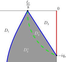
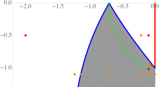
   Figure 2.1. Left: The third quadrant of the complex $k$-plane and the four regions $D_{1}$, $D_{2}^{+}$, $D_{2}^{-}$, $D_{3}$. Solid blue curve: $\mathop{\rm Im}[\theta(v_{o},k)]=0$; dashed green curve: the trace of the point $\bar{\alpha}$ (defined by (2.8)) as $\xi$ increases from $v_{o}$ to $0$. The case $p\in D_{1}$ corresponds to the transmission regime, the case $p\in D_{2}^{+}$ to the trap regime, the case $p\in D_{2}^{-}$ to the trap/wake regime, and the case $p\in D_{3}$ to the transmission/wake regime. Right: The different choices of the pole $p$ used in the numerical simulations of Figures 2.3, 2.4 (red dots) and 4.11 (orange dots).

10. We will show in Sections 4 and 5 that the third quadrant $\mathbb{C}_{\mathrm{iii}}$ of the complex $k$-plane is divided into the four regions $D_{1}$, $D_{2}^{+}$, $D_{2}^{-}$, $D_{3}$ defined as follows. Recall that, for a discrete eigenvalue at $k=p$, $v_{s}$ is uniquely defined as the value of $\xi$ such that $\mathop{\rm Im}[\theta(\xi,p)]=0$. Then, $\mathbb{C}_{\mathrm{iii}}$ can be decomposed into

    $$D_{1}\cup D_{3}=\left\{k\in\mathbb{C}_{\mathrm{iii}}:v_{s}<v_{o}<0\right\},$$

    $$D_{2}=\left\{k\in\mathbb{C}_{\mathrm{iii}}:0>v_{s}>v_{o}\right\}.$$

    These regions are shown in Figure 2.1 with $D_{1}\cup D_{3}$ in white and $D_{2}$ in gray. The solid blue curve separating them corresponds to the values of $k$ for which $v_{s}=v_{o}$ or, equivalently, to $\mathop{\rm Im}[\theta(v_{o},k)]=0$. The dashed green curve corresponds to the trace of the point $\bar{\alpha}$ as $\xi$ increases from $v_{o}$ to $0$.

    Note that:

    • The region where $v_{s}<v_{o}<0$ is divided by the blue curve $\mathop{\rm Im}[\theta(V_{o},k)]=0$ into two disjoint domains. Among them, we take $D_{1}$ to be the infinite domain and $D_{3}$ the one adjacent to the imaginary axis.

    • Similarly, the dashed green curve separates $D_{2}$ into two subdomains, $D_{2}^{+}$ and $D_{2}^{-}$, which we take as the portions of $D_{2}$ adjacent to $D_{1}$ and $D_{3}$, respectively.

    • We will show that $D_{1}$ and $D_{3}$ differ with respect to the number of solutions of equation (2.12) that arise in the interval $(v_{o},0)$. In particular, if $p\in D_{1}$ then (2.12) does not have a solution in $(v_{o},0)$, while if $p\in D_{3}$ then (2.12) possesses a unique solution $v_{w}\in(v_{o},0)$.

    • Similarly, we will show that if $p\in D_{2}^{+}$ then equation (2.12) possesses a unique solution $\widetilde{v}_{s}\in(v_{o},0)$ while if $p\in D_{2}^{-}$ then (2.12) has two solutions $\widetilde{v}_{s},v_{w}\in(v_{o},0)$ with $\widetilde{v}_{s}<v_{w}$.

The four interaction outcomes. Placing $p$ in each of the four regions $D_{1}$, $D_{2}^{+}$, $D_{2}^{-}$, $D_{3}$ gives rise to different, inequivalent asymptotic regimes, which we label as the transmission regime, the trap regime, the trap/wake regime, and the transmission/wake regime respectively.

Specifically, in Sections 4 and 5 we show that, depending on its location in the complex $k$-plane (see Figure 2.1), the presence of a discrete eigenvalue at $k=p$ gives rise to the following leading-order contributions in addition to the portion of the solution generated by the continuous spectrum:

1. In the transmission regime, i.e. when $p\in D_{1}$, a soliton along the ray $x=v_{s}t$;

2. In the trap regime, i.e. when $p\in D_{2}^{+}$, a soliton along the ray $x=\widetilde{v}_{s}t$;

3. In the trap/wake regime, i.e. when $p\in D_{2}^{-}$, a soliton along $x=\widetilde{v}_{s}t$ and a soliton wake along $x=v_{w}t$;

4. In the transmission/wake regime, i.e. when $p\in D_{3}$, a soliton along $x=v_{s}t$ and a soliton wake along $x=v_{w}t$.

In particular, we will see that the above outcomes are determined by whether there exist solutions of equation (2.11) for $\xi\in(-\infty,v_{o})$ and of equation (2.12) for $\xi\in(v_{o},0)$.

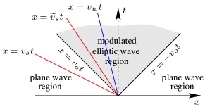
Figure 2.2. Asymptotically in time, the $xt$-plane is divided into the plane wave regions $|x|>|v_{o}|t$ and the modulated elliptic wave region $|x|<|v_{o}|t$. Also shown are the locations of the $O(1)$ contributions generated by a discrete eigenvalue at $k=p$ in the four inequivalent cases corresponding to the regions of Figure 2.1.

Long-time asymptotic results. We are now ready to give the precise form of the leading-order long-time asymptotics of the solution of the focusing NLS IVP (1.5) in each of the four inequivalent regimes described above. Numerical simulations with the discrete eigenvalue chosen in each of the four regions of Figure 2.1, illustrating the asymptotic results, are shown in Figures 2.3 and 2.4. For comparison purposes, Figures 2.3 and 2.4 also show the difference between $q(x,t)$ and the solution $q_{\mathrm{wedge}}(x,t)$ produced by an initial condition that generates the same reflection coefficient as $f(x)$ but no discrete spectrum. The numerical methods used in the numerical simulations were described in [BLM2]. Recall that, since we are taking $\mathop{\rm Re}(p)<0$, all relevant velocities and all values of $\xi$ considered in Theorems 2.1–2.4 below are negative.

Theorem 2.1 (Transmission regime).

Suppose $p\in D_{1}$ and let $v_{s}<v_{o}<0$ be defined by (2.10). Then the solution $q(x,t)$ of the focusing NLS IVP (1.5) exhibits the following asymptotic behavior as $t\to\infty$. (i) If $\xi<v_{s}$, then the leading-order asymptotics is described by the plane wave

$$q(x,t)=q_{\textnormal{pw}}(\xi)+O\big{(}t^{-\frac{1}{2}}\big{)},\quad t\to\infty,$$ (2.14)

where

$$q_{\textnormal{pw}}(\xi):=q_{-}\,e^{2ig_{\infty}(\xi)}$$ (2.15)

and the real, constant phase $g_{\infty}(\xi)$ is given by (4.66). (ii) If $\xi=v_{s}$, then the leading-order asymptotics is equal to a soliton on top of a nonzero plane-wave background, i.e.

$$q(x,t)=q_{\textnormal{pw}}(v_{s})+q_{s}(t)\,e^{2ig_{\infty}(v_{s})}+O\big{(}t^{-\frac{1}{2}}\big{)},\quad t\to\infty,$$ (2.16)

with $q_{\textnormal{pw}}$ given by (2.15), $g_{\infty}(v_{s})$ defined by (4.66), and the soliton $q_{s}$ given by

$$q_{s}(t)=\frac{\left|R_{p}\right|\left(\bar{\mathcal{A}}\Lambda_{1}^{2}\bar{q}_{-}+\mathcal{A}\Lambda_{2}^{2}q_{-}-2\mathcal{B}\Lambda_{1}\Lambda_{2}q_{o}\right)+e^{i\left[2\theta(v_{s},p)t+\arg(R_{p})\right]}\Lambda_{1}^{2}\bar{q}_{-}+e^{-i\left[2\theta(v_{s},p)t+\arg(R_{p})\right]}\Lambda_{2}^{2}q_{-}}{4i\bar{q}_{-}\left\{\sqrt{|\mathcal{A}|^{2}-\mathcal{B}^{2}}\cosh\big{[}\ln\big{(}|R_{p}|\sqrt{|\mathcal{A}|^{2}-\mathcal{B}^{2}}\,\big{)}\big{]}+\mathop{\rm Re}\big{(}\mathcal{A}e^{i\left[2\theta(v_{s},p)t+\arg(R_{p})\right]}\big{)}\right\}}$$ (2.17)

with the constants $R_{p}$, $(\mathcal{A},\mathcal{B})$ and $(\Lambda_{1},\Lambda_{2})$ given by (4.75cf), (4.75cs) and (4.75da) respectively. (iii) If $v_{s}<\xi<v_{o}$, then the leading-order asymptotics is given by the plane wave (2.14) up to a constant phase shift, namely

$$q(x,t)=q_{\textnormal{pw}}(\xi)\,e^{4i\,\textnormal{arg}\left[p+\lambda(p)\right]}+O\big{(}t^{-\frac{1}{2}}\big{)},\quad t\to\infty.$$ (2.18)

(iv) Finally, if $v_{o}<\xi<0$, then the asymptotic behavior of the solution is described at leading order by the phase-shifted modulated elliptic wave

$$q(x,t)=\widetilde{q}_{\textnormal{mew}}(x,t)\,e^{4i\,\textnormal{arg}\left[p+\lambda(p)\right]}+O\big{(}t^{-\frac{1}{2}}\big{)},\quad t\to\infty,$$ (2.19)

where

$$\widetilde{q}_{\textnormal{mew}}(x,t)=\frac{q_{o}\left(q_{o}+\alpha_{\textnormal{im}}\right)}{\bar{q}_{-}}\ \frac{\Theta\Big{(}\frac{\sqrt{q_{o}\alpha_{\textnormal{im}}}}{mK(m)}\left(x-2\alpha_{\textnormal{re}}t\right)-X_{o}+2\upnu_{\infty}-\frac{1}{2}-\frac{\widetilde{\omega}}{2\pi}\Big{)}\Theta\left(\frac{1}{2}\right)}{\Theta\Big{(}\frac{\sqrt{q_{o}\alpha_{\textnormal{im}}}}{mK(m)}\left(x-2\alpha_{\textnormal{re}}t\right)-X_{o}-\frac{1}{2}-\frac{\widetilde{\omega}}{2\pi}\Big{)}\Theta\left(2\upnu_{\infty}-\frac{1}{2}\right)}\,e^{2i\left[g_{\infty}(\xi)-G_{\infty}(\xi)t\right]}$$ (2.20)

with the Jacobi function $\Theta$ defined by (4.75hvid), the complex quantity $\upnu_{\infty}$ given by (4.75hvii), and the real quantities $G_{\infty}$, $g_{\infty}$, $X_{o}$ and $\widetilde{\omega}$ defined by equations (4.75go), (4.75gw), (4.75hvir) and (4.75hi) respectively. Importantly, all of these quantities depend on $x$ and $t$ only through the similarity variable $\xi$.

Theorem 2.2 (Trap regime).

Suppose $p\in D_{2}^{+}$ and let $\widetilde{v}_{s}$ be the unique solution of equation (2.12) in the interval $(v_{o},0)$. Then the solution $q(x,t)$ of the focusing NLS IVP (1.5) exhibits the following asymptotic behavior as $t\to\infty$. (i) If $\xi<v_{o}$, then the leading-order asymptotics is given by the plane wave (2.14). (ii) If $v_{o}<\xi<\widetilde{v}_{s}$, then the leading-order asymptotics is described by the modulated elliptic wave

$$q(x,t)=q_{\textnormal{mew}}(x,t)+O\big{(}t^{-\frac{1}{2}}\big{)},\quad t\to\infty,$$ (2.21)

where $q_{\textnormal{mew}}$ is obtained from (2.20) after setting $\widetilde{\omega}=0$, i.e.

$$q_{\textnormal{mew}}(x,t)=\frac{q_{o}\left(q_{o}+\alpha_{\textnormal{im}}\right)}{\bar{q}_{-}}\ \frac{\Theta\Big{(}\frac{\sqrt{q_{o}\alpha_{\textnormal{im}}}}{mK(m)}\left(x-2\alpha_{\textnormal{re}}t\right)-X_{o}+2\upnu_{\infty}-\frac{1}{2}\Big{)}\Theta\left(\frac{1}{2}\right)}{\Theta\Big{(}\frac{\sqrt{q_{o}\alpha_{\textnormal{im}}}}{mK(m)}\left(x-2\alpha_{\textnormal{re}}t\right)-X_{o}-\frac{1}{2}\Big{)}\Theta\left(2\upnu_{\infty}-\frac{1}{2}\right)}\,e^{2i\left[g_{\infty}(\xi)-G_{\infty}(\xi)t\right]}.$$ (2.22)

(iii) If $\xi=\widetilde{v}_{s}$, then at leading order the asymptotics is equal to a soliton on top of a nonzero modulated-elliptic-wave background, i.e.

$$q(x,t)=q_{\textnormal{mew}}(\widetilde{v}_{s}t,t)+q_{p}(t)+O\big{(}t^{-\frac{1}{2}}\big{)},\quad t\to\infty,$$ (2.23)

where the modulated elliptic wave $q_{\textnormal{mew}}$ is defined by (2.22) and the soliton $q_{p}$ is given by

$$q_{p}(t)=2i\,\frac{2\mathcal{B}\rho_{p}\rho_{\bar{p}}W_{11}(p)W_{12}(\bar{p})-\left(1+\mathcal{C}\rho_{\bar{p}}\right)\rho_{p}W_{11}(p)^{2}+\left(1+\mathcal{A}\rho_{p}\right)\rho_{\bar{p}}W_{12}(\bar{p})^{2}}{\mathcal{B}^{2}\rho_{p}\rho_{\bar{p}}+\left(1+\mathcal{C}\rho_{\bar{p}}\right)\left(1+\mathcal{A}\rho_{p}\right)}$$ (2.24)

with $(\rho_{p},\rho_{\bar{p}})$, $W$ and $(\mathcal{A},\mathcal{B},\mathcal{C})$ given by (4.75hvkq), (4.75hvku) and (4.75hvkab) respectively. (iv) Finally, if $\widetilde{v}_{s}<\xi<0$, then the asymptotics is given by the phase-shifted modulated elliptic wave (2.19).

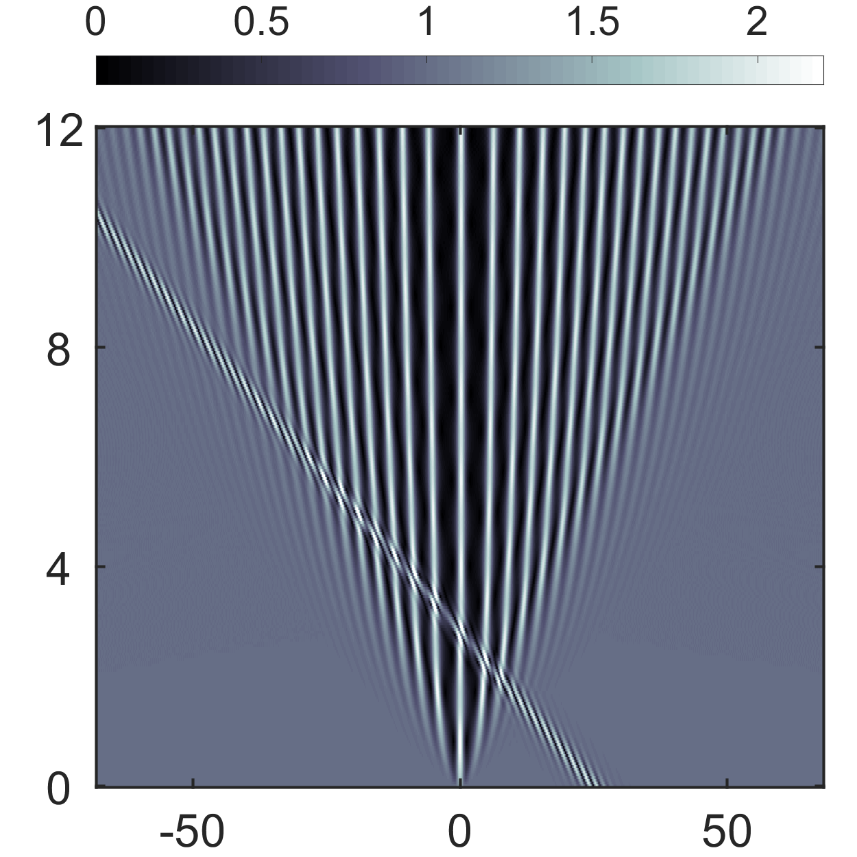
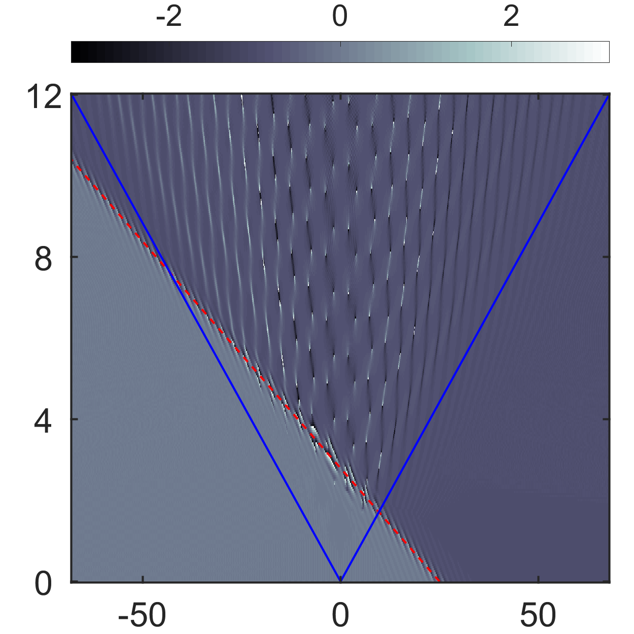
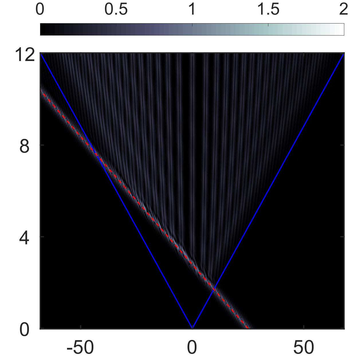
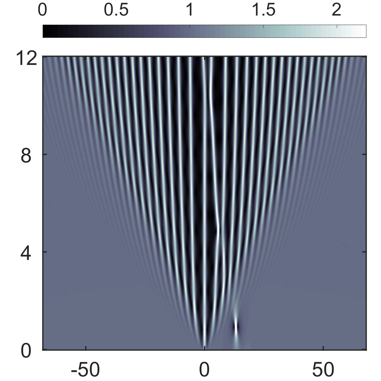
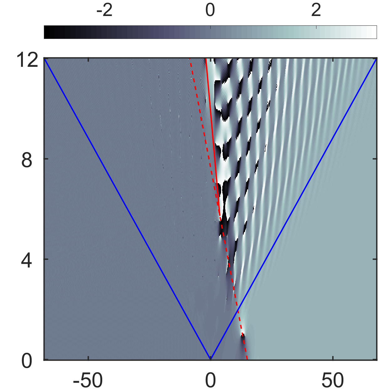
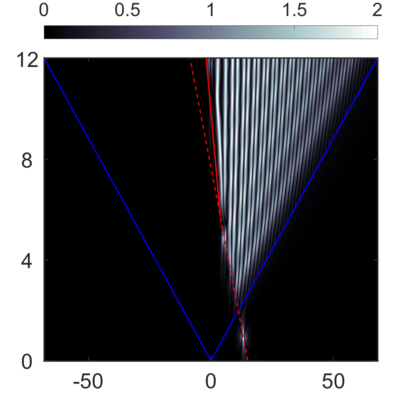
Figure 2.3. Numerical solutions of the IVP (1.5) with $q_{o}=1$ and different choices of $p$ for the two pure asymptotic regimes (red dots in Figure 2.1). Top row: Transmission regime (Theorem 2.1) with $p=-2-0.5i\in D_{1}$. Bottom row: Trap regime (Theorem 2.2) with $p=-0.1-1.02i\in D_{2}^{+}$. In all cases, the horizontal axis corresponds to $x$ and the vertical axis to $t$. The grayscale used in the plots is shown in the top inserts. Left column: Density plots of the solution amplitude $|q(x,t)|$. Center column: The complex phase difference between the solution in the left column and the solution $q_{\mathrm{wedge}}(x,t)$ generated just by the localized disturbance (i.e. without the soliton), illustrating the asymptotic phase shift as $x\to\pm\infty$ induced by the soliton. Right column: The amplitude difference between the solution in the left column and $q_{\mathrm{wedge}}(x,t)$, illustrating the asymptotic position shift introduced by the soliton. Blue lines: The boundary $x=\pm v_{o}t$ between the wedge of modulated periodic oscillations from the left and right plane wave regions. Dashed red lines: The original soliton trajectory (velocity $v_{s}$). Solid red lines: The final soliton trajectory (which is either $v_{s}$ or $\widetilde{v}_{s}$ depending on the regime). The position shift is very small in the transmission regime but becomes more noticeable in the trap regime. In both cases, the position shift is confined to the portion of the wedge lying above the soliton, in agreement with Theorems 2.1 and 2.2.

Theorem 2.3 (Trap/wake regime).

Suppose $p\in D_{2}^{-}$ and let $\widetilde{v}_{s}<v_{w}$ be the two solutions of equation (2.12) in the interval $(v_{o},0)$. Then, the solution $q(x,t)$ of the focusing NLS IVP (1.5) exhibits the following asymptotic behavior as $t\to\infty$. (i) If $\xi<v_{o}$, then the leading-order asymptotics is described by the plane wave (2.14). (ii) If $v_{o}<\xi<\widetilde{v}_{s}$, then the leading-order asymptotics is given by the modulated elliptic wave (2.21). (iii) If $\xi=\widetilde{v}_{s}$, then the asymptotics is characterized by (2.23), namely at leading order it is equal to the sum of the modulated elliptic wave (2.22) evaluated at $x=\widetilde{v}_{s}t$ and the soliton (2.24). (iv) If $\widetilde{v}_{s}<\xi<v_{w}$, then the leading-order asymptotics is given by the phase-shifted modulated elliptic wave (2.19). (v) If $\xi=v_{w}$, then at leading order the asymptotics is equal to a soliton wake on top of a nonzero modulated-elliptic-wave background, i.e.

$$q(x,t)=q_{\textnormal{mew},w}(t)+q_{w}(t)+O\big{(}t^{-\frac{1}{2}}\big{)},\quad t\to\infty,$$ (2.25)

where the modulated elliptic wave $q_{\textnormal{mew},w}(t)$ is given by (2.22) evaluated at $x=v_{w}t$ but with $\omega$ in $X_{o}$ replaced by $\omega_{w}$ of (4.75hvki) and with $g_{\infty}$ replaced by $g_{w,\infty}$ of (4.75hvkm), and the soliton wake $q_{w}$ is defined by

$$q_{w}(t):=2i\,\frac{2\mathcal{B}_{w}{\rho_{p}}_{w}{\rho_{\bar{p}}}_{w}{W_{w}}_{11}(\bar{p}){W_{w}}_{12}(p)-\big{(}1+\mathcal{C}_{w}{\rho_{p}}_{w}\big{)}{\rho_{\bar{p}}}_{w}{W_{w}}_{11}(\bar{p})^{2}+\big{(}1+\mathcal{A}_{w}{\rho_{\bar{p}}}_{w}\big{)}{\rho_{p}}_{w}{W_{w}}_{12}(p)^{2}}{\mathcal{B}_{w}^{2}{\rho_{p}}_{w}{\rho_{\bar{p}}}_{w}+\big{(}1+\mathcal{C}_{w}{\rho_{p}}_{w}\big{)}\big{(}1+\mathcal{A}_{w}{\rho_{\bar{p}}}_{w}\big{)}},$$ (2.26)

with $({\rho_{p}}_{w},{\rho_{\bar{p}}}_{w})$, $W_{w}$ and $(\mathcal{A}_{w},\mathcal{B}_{w},\mathcal{C}_{w})$ given by (4.75hvkv), (4.75hvkaa) and (4.75hvkag) respectively. (vi) Finally, if $v_{w}<\xi<0$, then the leading-order asymptotics is the same with the one in the range $\widetilde{v}_{s}<\xi<v_{w}$, namely it is given by the phase-shifted modulated elliptic wave (2.19).

Theorem 2.4 (Transmission/wake regime).

Suppose $p\in D_{3}$, let $v_{s}<v_{o}<0$ be defined by (2.10), and let $v_{w}$ be the unique solution of equation (2.12) in the interval $(v_{o},0)$. Then, the solution $q(x,t)$ of the focusing NLS IVP (1.5) exhibits the following asymptotic behavior as $t\to\infty$. (i) If $\xi<v_{s}$, then the leading-order asymptotics is given by the plane wave (2.14). (ii) If $\xi=v_{s}$, then the asymptotics is characterized by (2.16), namely at leading order it is given by the superposition of the plane wave (2.15) and the soliton (2.17). (iii) If $v_{s}<\xi<v_{o}$, then the leading-order asymptotics is described by the phase-shifted plane wave (2.18). (iv) If $v_{o}<\xi<v_{w}$, then the leading-order asymptotics is given by the phase-shifted modulated elliptic wave (2.19). (v) If $\xi=v_{w}$, then the asymptotics is characterized by (2.25), i.e. at leading order it is equal to the sum of the modulated elliptic wave $q_{\text{mew},w}(t)$ and the soliton wake (2.26). (vi) Finally, if $v_{w}<\xi<0$, then the leading-order asymptotics is the same with the one in the range $v_{o}<\xi<v_{w}$, namely it is given by the phase-shifted modulated elliptic wave (2.19).

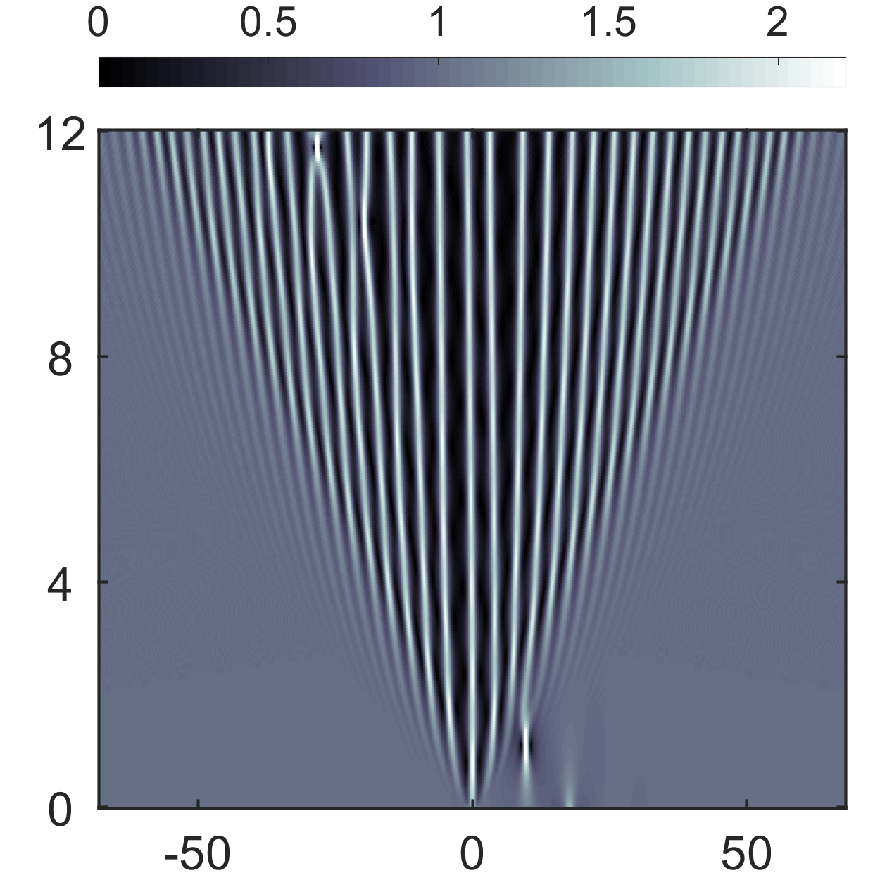
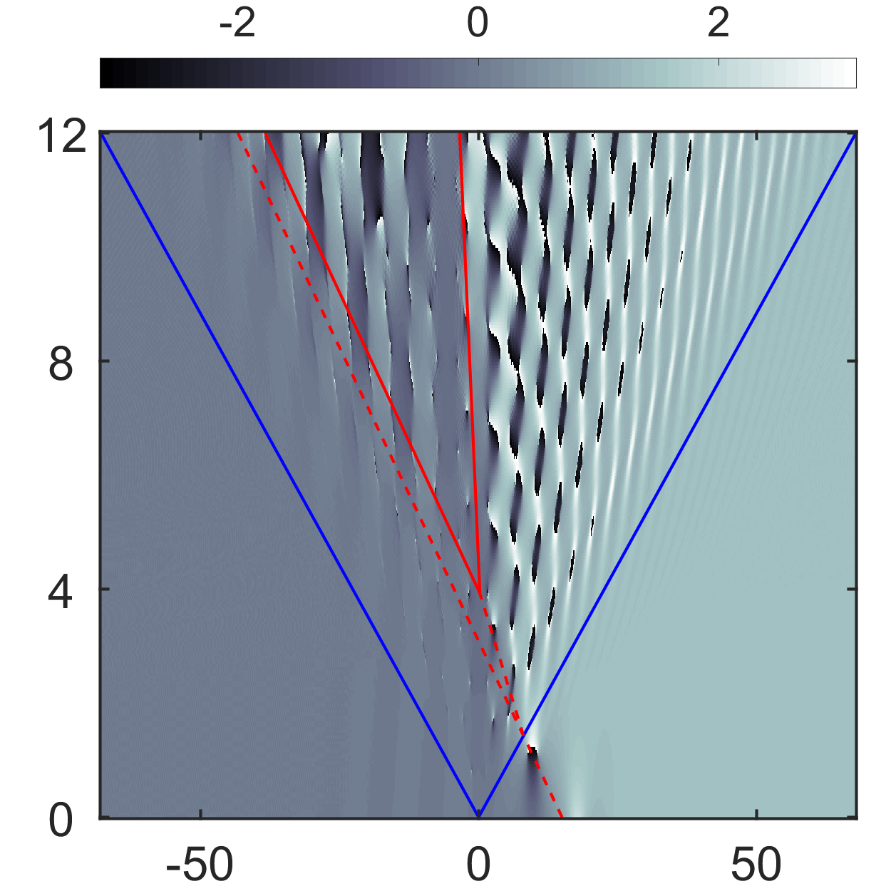
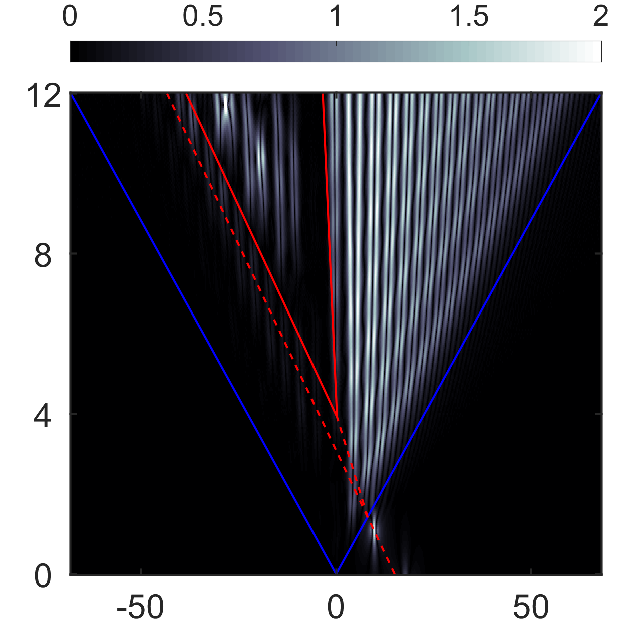
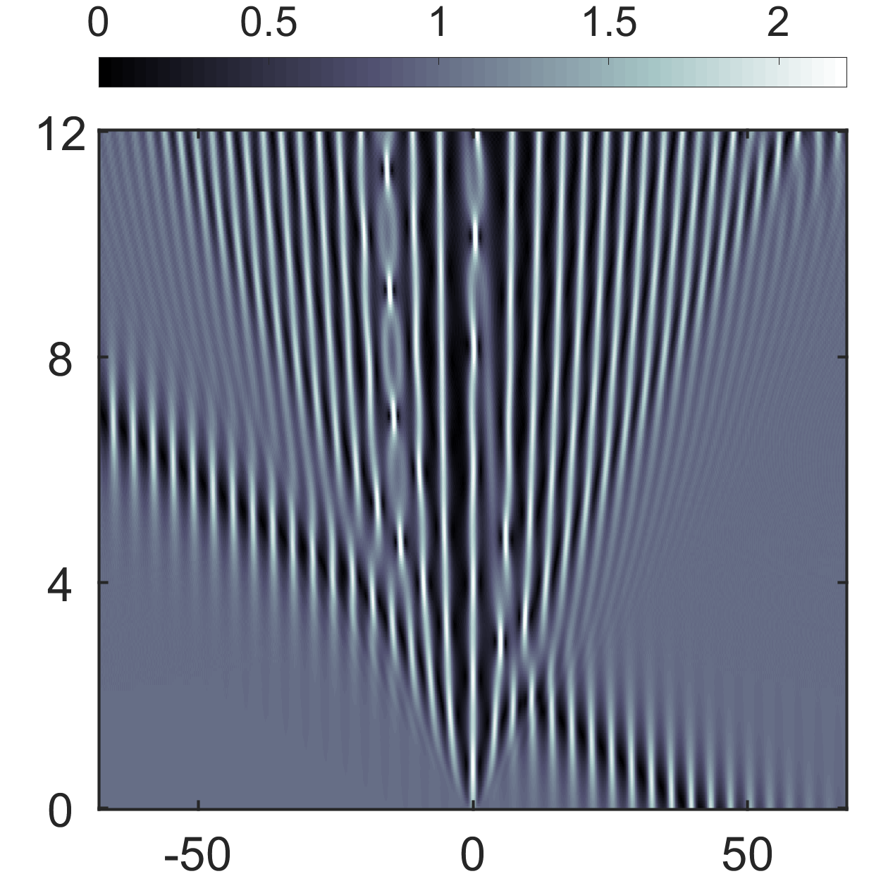
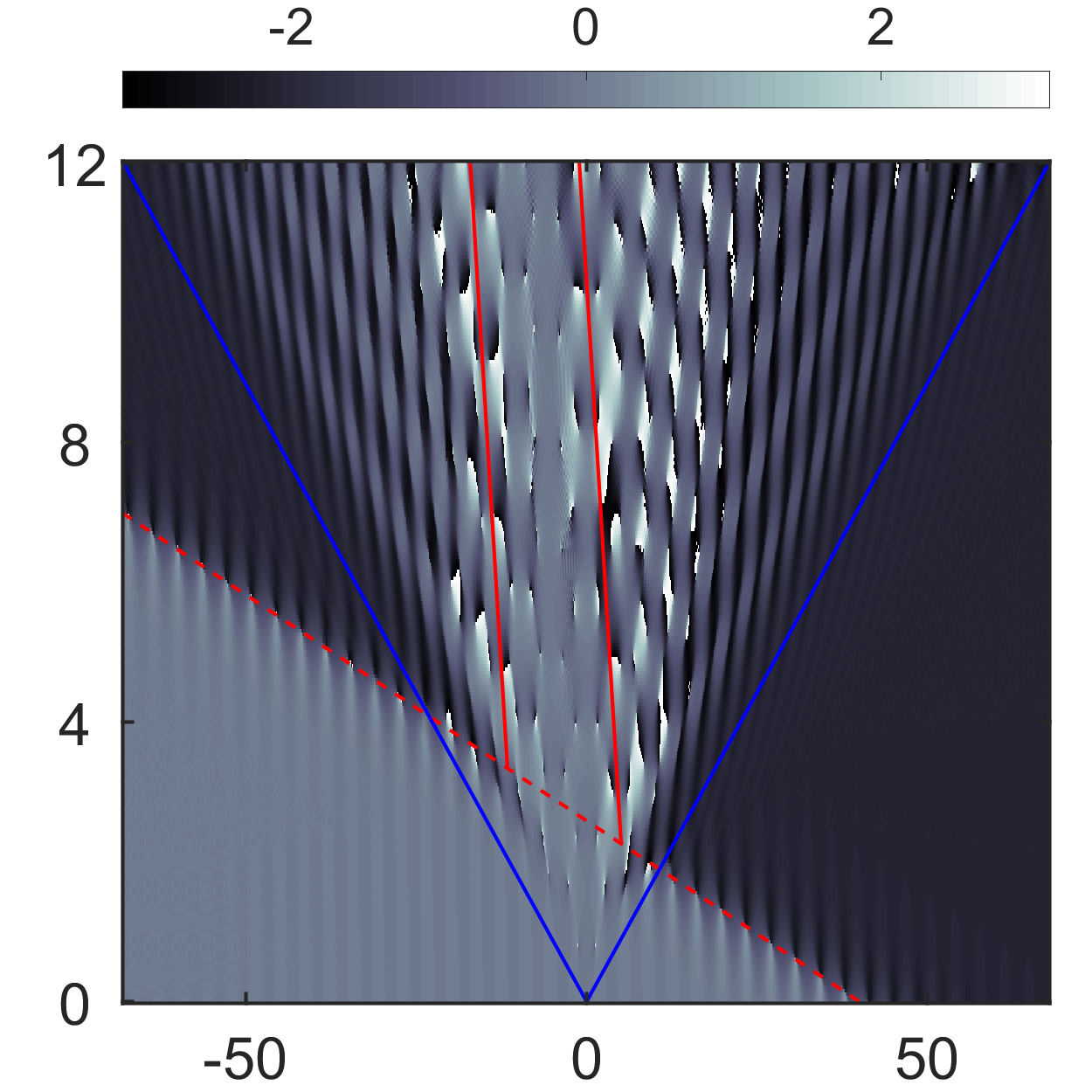
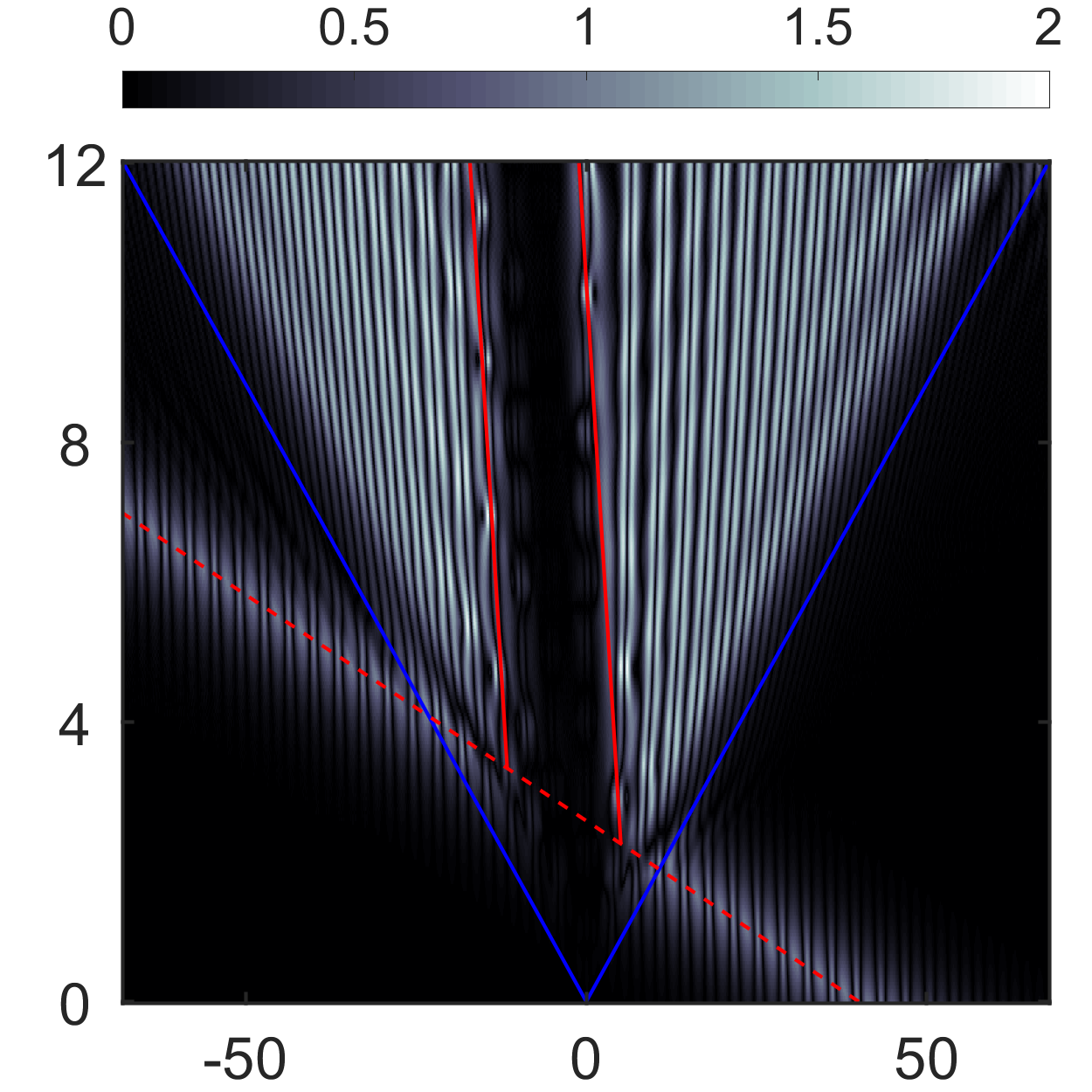
Figure 2.4. The analogue of Figure 2.3 for $p$ corresponding to the two mixed asymptotic regimes (orange dots in Figure 2.1). Here, the solid red lines also identify the soliton wakes, propagating with velocity $v_{w}$, where $|v_{w}|<|\widetilde{v}_{s}|<|v_{s}|$. Top row: Trap/wake regime (Theorem 2.3) with $p=-0.05-0.95i\in D_{2}^{-}$. Bottom row: Transmission/wake regime (Theorem 2.4) with $p=-0.1-0.5i\in D_{3}$. Note that the choice of $p$ in the trap/wake regime is very close to the boundary between $D_{2}^{-}$ and $D_{3}$ and, as a result, the dashed and solid red lines corresponding respectively to the original and modified soliton velocities are almost identical. Moreover, note that the two wakes seen in the transmission/wake regime have the same speed, and hence are detected as a single wake in the asymptotic analysis, which is why no wake-induced phase or position shift is observed in the asymptotics for $\xi>v_{w}$.

Remark 2.1 (Leading-order asymptotics for $x>0$).

Since the pole $p$ lies in the third quadrant of the complex $k$-plane, it has no effect on the asymptotics for $x>0$ (equivalently, $\xi>0$; see Figure 3.2). In particular, for $x>0$ the leading-order asymptotics of IVP (1.5) is described by Theorems 1.1 and 1.2 of [BM2], the only difference being that now one must also include the constant phase shift $4\textnormal{arg}\left[p+\lambda(p)\right]$ and the position shift induced by the soliton arising for $x<0$.

Remark 2.2.

In the appendix, we explicitly verify that the expression (2.17) for the soliton obtained in the long-time asysmptotics agrees with the long-time asymptotics of the standard soliton solution of the focusing NLS with nonzero background.

Remark 2.3 (Soliton versus soliton wake).

The soliton arising either at $\xi=v_{s}$ or at $\xi=\widetilde{v}_{s}$ induces a constant phase shift (equal to $4\textnormal{arg}\left[p+\lambda(p)\right]$) as well as a position shift (related to the presence of $\widetilde{\omega}$ in (2.20) as opposed to (2.22)) in the leading-order asymptotics for subsequent values of $\xi$. On the contrary, the soliton wake arising at $\xi=v_{w}$ has no effect on the leading-order asymptotics for $\xi>v_{w}$. The numerical simulations of Figures 2.3 and 2.4 illustrate these remarks.

Remark 2.4 (Multiple leading-order contributions from the poles).

We find it quite remarkable that in the two mixed regimes a single pair of complex conjugate poles produces $O(1)$ contributions to the solution at two different velocities: the soliton velocity and the wake velocity, as specified in Theorems 2.3 and 2.4. (These predictions are validated by the numerical results in Figures 2.3 and 2.4.) To the best of our knowledge, this is the first time that such a phenomenon has been observed in the long-time asymptotic analysis of an integrable system, and is perhaps one of the main novelties in the results of the present work. Moreover, the numerical results in the bottom row of Figure 2.4 suggest that the soliton-generated wake may comprise itself two different localized structures. We emphasize however that, since these two structures propagate with the same velocity, in order to be able to differentiate between them one would have to compute the asymptotics by taking $x=\xi t+y$. Such a calculation is outside the scope of this work.

Structure of the paper. In Section 3, the solution of IVP (1.5) for the focusing NLS equation is associated with the solution of a matrix Riemann-Hilbert problem via the inverse scattering transform. Furthermore, the four different long-time asymptotic patterns, namely the transmission, trap, trap/wake, and transmission/wake regimes, are motivated through the behavior of the jump matrices of this Riemann-Hilbert problem. The transmission regime is analyzed in Section 4, resulting in the proof of Theorem 2.1. The proof of Theorem 2.2 for the trap regime is provided in Section 5. The two mixed regimes are discussed in Section 6, leading to the proofs of Theorems 2.3 and 2.4. Finally, some concluding remarks are given in Section 7.

3. The Riemann-Hilbert Problem and Outline of the Asymptotic Analysis

The implementation of the inverse scattering transform method for IVP (1.5) begins with the integration of the Lax pair (1.6) for the $2\times 2$ matrix-valued function $\Psi$ assuming as usual that the solution $q$ of problem (1.5) is given. This task is known as the direct problem. Then, $q$ is expressed in terms of a sectionally meromorphic function $M$ which is defined via appropriate combinations of the two column vectors $\Psi_{1}$ and $\Psi_{2}$ of $\Psi$, and which satisfies a certain matrix Riemann-Hilbert problem. This portion of the analysis is known as the inverse problem. Specifically, the discussion of the direct problem in Section 2 of [BM2] motivates the following definition for the sectionally meromorphic matrix-valued function $M$:

$$M(x,t,k)=\left\{\begin{array}[]{ll}\left(\dfrac{\Psi_{+1}(x,t,k)}{\bar{a}(k)d(k)},\Psi_{-2}(x,t,k)\right)e^{-i\theta(\xi,k)t\sigma_{3}},&k\in\mathbb{C}^{+}\setminus B^{+},\\ \left(\Psi_{-1}(x,t,k),\dfrac{\Psi_{+2}(x,t,k)}{a(k)d(k)}\right)e^{-i\theta(\xi,k)t\sigma_{3}},&k\in\mathbb{C}^{-}\setminus B^{-}.\end{array}\right.$$ (3.1)

In the above definition, we use the notation

$$\mathbb{C}^{\pm}:=\left\{k\in\mathbb{C}:\mathop{\rm Im}(k)\gtrless 0\right\},\quad B^{+}:=i\left[0,q_{o}\right],\quad B^{-}:=i\left[-q_{o},0\right]$$

and denote by $\Psi_{\pm}$ the so-called Jost solutions, namely the simultaneous solutions of the Lax pair (1.6) with prescribed normalizations as $x\to\pm\infty$:

$$\Psi_{\pm}(x,t,k)=\begin{pmatrix}1&{i(\lambda-k)}/{\bar{q}_{\pm}}\\ {i(\lambda-k)}/{q_{\pm}}&1\end{pmatrix}e^{i\theta(\xi,k)t\sigma_{3}}\left[1+o(1)\right],\quad x\to\pm\infty.$$ (3.2)

(Recall that the quantities $\lambda$, $\theta$ and $\xi$ are defined by (2.2), (2.3) and (2.4) respectively.) Furthermore, we define the spectral function $a(k)$ along with its Schwarz conjugate $\bar{a}(k)$ by

$$a(k)=\frac{\text{wr}\left[\Psi_{-1}(x,t,k),\Psi_{+2}(x,t,k)\right]}{d(k)},\quad\bar{a}(k):=\overline{a(\bar{k})}=\frac{\text{wr}\left[\Psi_{+1}(x,t,k),\Psi_{-2}(x,t,k)\right]}{d(k)},$$ (3.3)

where “wr” denotes the Wronskian determinant and

$$d(k):=\frac{2\lambda(k)}{\lambda(k)+k}.$$ (3.4)

Importantly, the Wronskian determinants appearing in (3.3) are independent of $x$ and $t$, and hence the functions $a$ and $\bar{a}$ depend only on $k$.

The definition (3.1) of $M$, in combination with the analyticity properties of $\Psi_{\pm}$ (see [BM2] for more details), implies that the only sources of nonanalyticity of $M$ are

1. the continuous spectrum

   $$\Sigma:=\mathbb{R}\cup B,$$ (3.5)

   along which $M$ exhibits jump discontinuities, and

2. the possible zeros of the spectral function $a(k)$, which form the discrete spectrum of the Riemann-Hilbert problem satisfied by $M$.

It was shown in [BM2] that, if there is no discrete spectrum, namely, if

$$a(k)\neq 0\quad\forall k\in\mathbb{C}^{-}\cup\Sigma,$$ (3.6)

then the function $M(x,t,k)$ satisfies the following Riemann-Hilbert problem:

$$M^{+} =M^{-}V_{1}, k\in\mathbb{R},$$ (3.7a)

$$M^{+} =M^{-}V_{2}, k\in B^{+},$$ (3.7b)

$$M^{+} =M^{-}V_{3}, k\in B^{-},$$ (3.7c)

$$M =I+O\left(\tfrac{1}{k}\right),\quad k\to\infty,$$ (3.7d)

where the jump matrices along the three contours $\mathbb{R}$, $B^{+}$, $B^{-}$ comprising the continuous spectrum $\Sigma$ are given by (see Figure 3.1)

$$V_{1}(x,t,k) =\left(\begin{array}[]{lr}\dfrac{1}{d(k)}\left[1+r(k)\bar{r}(k)\right]&\bar{r}(k)e^{2i\theta(\xi,k)t}\\ r(k)e^{-2i\theta(\xi,k)t}&d(k)\end{array}\right),$$ (3.8c)

$$V_{2}(x,t,k) =\left(\begin{array}[]{lr}-\dfrac{\lambda(k)-k}{iq_{-}}\,\bar{r}(k)\,e^{2i\theta(\xi,k)t}&\dfrac{2\lambda(k)}{i\bar{q}_{-}}\\ \dfrac{\bar{q}_{-}}{2i\lambda(k)}\left[1+r(k)\bar{r}(k)\right]&-\dfrac{\lambda(k)+k}{i\bar{q}_{-}}\,r(k)\,e^{-2i\theta(\xi,k)t}\end{array}\right),$$ (3.8f)

$$V_{3}(x,t,k) =\left(\begin{array}[]{lr}\dfrac{\lambda(k)+k}{iq_{-}}\,\bar{r}(k)\,e^{2i\theta(\xi,k)t}&\dfrac{q_{-}}{2i\lambda(k)}\left[1+r(k)\bar{r}(k)\right]\\ \dfrac{2\lambda(k)}{iq_{-}}&\dfrac{\lambda(k)-k}{i\bar{q}_{-}}\,r(k)\,e^{-2i\theta(\xi,k)t}\end{array}\right),$$ (3.8i)

with the reflection coefficient $r$ defined by

$$r(k)=-\frac{b(k)}{\bar{a}(k)},\quad b(k):=\frac{\text{wr}\left[\Psi_{+1}(x,t,k),\Psi_{-1}(x,t,k)\right]}{d(k)}.$$ (3.9)

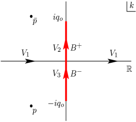
Figure 3.1. The branch cut $B=B^{+}\cup B^{-}$, the jumps $V_{1}$, $V_{2}$, $V_{3}$ of Riemann-Hilbert problem (3.7), and the conjugate pair of simple poles $p,\bar{p}$.

Removing the assumption (3.6), i.e. allowing the spectral function $a(k)$ to vanish in $\mathbb{C}^{-}$, results in a Riemann-Hilbert problem with a nonempty discrete spectrum. In this work, we consider the simplest such scenario, according to which the initial data ${f}(x)$ of IVP (1.5) is such that $a(k)$ has a unique, simple zero in $\mathbb{C}^{-}\setminus\Sigma$. That is, we assume that there exists a unique $p\in\mathbb{C}^{-}\setminus\Sigma$ such that $a(p)=0$ and, furthermore, $a^{\prime}(p)\neq 0$. Correspondingly, the Schwarz conjugate $\bar{a}(k)$ of $a(k)$ possesses a unique, simple zero $\bar{p}\in\mathbb{C}^{+}\setminus\Sigma$ and, by definition (3.1), $M$ is meromorphic in $\mathbb{C}\setminus\Sigma$ with two simple poles, at $k=p$ and at $k=\bar{p}$. Therefore, in addition to the jumps $V_{1},V_{2},V_{3}$ along the continuous spectrum $\Sigma$, the Riemann-Hilbert problem for $M$ must be supplemented by suitable residue conditions at $p$ and $\bar{p}$. These can be computed as follows.

Since $a(p)=0$, by expression (3.3) we have that $\text{wr}\left[\Psi_{-1}(x,t,p),\Psi_{+2}(x,t,p)\right]=0$ for all $x,t\in\mathbb{R}$. In turn, since neither $\Psi_{-1}(x,t,p)$ nor $\Psi_{+2}(x,t,p)$ can be identically zero due to the normalization (3.2), we infer that there exists a constant $C_{p}\neq 0$ such that

$$\Psi_{+2}(x,t,p)=C_{p}\Psi_{-1}(x,t,p)\quad\forall x,t\in\mathbb{R}.$$ (3.10a)

Similarly, evaluating (3.3) at $$k=\bar{p}$$ we obtain

$$\Psi_{+1}(x,t,\bar{p})=C_{\bar{p}}\Psi_{-2}(x,t,\bar{p})\quad\forall x,t\in\mathbb{R}$$ (3.10b)

for some constant $C_{\bar{p}}\neq 0$. Thus,

$$\underset{k=p}{\text{Res}}\,\frac{\Psi_{+2}(x,t,k)}{a(k)d(k)}=\frac{\Psi_{+2}(x,t,p)}{a^{\prime}(p)d(p)}=c_{p}\Psi_{-1}(x,t,p)\quad\forall x,t\in\mathbb{R},\quad c_{p}:=\frac{C_{p}}{a^{\prime}(p)d(p)}.$$ (3.11a)

$$\underset{k=\bar{p}}{\text{Res}}\,\frac{\Psi_{+1}(x,t,k)}{\bar{a}(k)d(k)}=\frac{\Psi_{+1}(x,t,\bar{p})}{\bar{a}^{\prime}(\bar{p})d(\bar{p})}=c_{\bar{p}}\Psi_{-2}(x,t,\bar{p})\quad\forall x,t\in\mathbb{R},\quad c_{\bar{p}}:=\frac{C_{\bar{p}}}{\bar{a}^{\prime}(\bar{p})d(\bar{p})}.$$ (3.11b)

Relations (3.11a) and (3.11b) imply the following residue conditions for $M$:

$$\underset{k=p}{\text{Res}}\,M(x,t,k)=M(x,t,p)\left(\begin{array}[]{lr}0&c_{p}\,e^{2i\theta(\xi,p)t}\\ 0&0\end{array}\right) \forall x,t\in\mathbb{R},$$ (3.12c)

$$\underset{k=\bar{p}}{\text{Res}}\,M(x,t,k)=M(x,t,\bar{p})\left(\begin{array}[]{lr}0&0\\ c_{\bar{p}}\,e^{-2i\theta(\xi,\bar{p})t}&0\end{array}\right)\quad \forall x,t\in\mathbb{R}.$$ (3.12f)

The Riemann-Hilbert problem for the focusing NLS IVP (1.5) in the presence of the discrete spectrum $\{p,\bar{p}\}$ comprises the empty-discrete-spectrum problem (3.7) augmented with the residue conditions (3.12). To ensure uniqueness of solutions of the above Riemann-Hilbert problem, one must also supplement it with suitable growth conditions at the branch points [BMi].

The $x$-part of the Lax pair (1.6) together with the definition (3.1) and the asymptotic condition (3.16f) yield the solution of the IVP (1.5) via the reconstruction formula

$$q(x,t)=-2i\lim_{k\to\infty}kM_{12}(x,t,k).$$ (3.13)

For the purpose of computing the long-time asymptotics, it is convenient to convert the residue conditions (3.12) into jump discontinuities. In particular, following [Mi], we let $\partial D_{p}^{\varepsilon}$ and $\partial D_{\bar{p}}^{\varepsilon}$ be the positively oriented boundaries of the disks $D_{p}^{\varepsilon}$ and $D_{\bar{p}}^{\varepsilon}$ of radius $\varepsilon$ centered at $p$ and $\bar{p}$ respectively, and define the function $N$ by

$$N(x,t,k)=\begin{cases}M(x,t,k)V_{p}(x,t,k),&k\in D_{p}^{\varepsilon},\\ M(x,t,k),&k\in\mathbb{C}^{-}\setminus\left(B^{-}\cup\overline{D_{p}^{\varepsilon}}\,\right),\\ M(x,t,k)V_{\bar{p}}(x,t,k),&k\in D_{\bar{p}}^{\varepsilon},\\ M(x,t,k),&k\in\mathbb{C}^{+}\setminus\left(B^{+}\cup\overline{D_{\bar{p}}^{\varepsilon}}\,\right),\end{cases}$$ (3.14)

where the matrices $V_{p}$ and $V_{\bar{p}}$ are given by

$$V_{p}(x,t,k)=\left(\begin{array}[]{lr}1&-\dfrac{c_{p}}{k-p}\,e^{2i\theta(\xi,p)t}\\ 0&1\end{array}\right),\quad V_{\bar{p}}(x,t,k)=\left(\begin{array}[]{lr}1&0\\ -\dfrac{c_{\bar{p}}}{k-\bar{p}}\,e^{-2i\theta(\xi,\bar{p})t}&1\end{array}\right).$$ (3.15)

Note that the residue conditions (3.12) imply that $N$ is analytic at $p$ and $\bar{p}$. Furthermore, the jumps of $N$ along the continuous spectrum $\Sigma$ are the same with those of $M$ since $N=M$ outside the disks $D_{p}^{\varepsilon}$ and $D_{\bar{p}}^{\varepsilon}$. Therefore, $N(x,t,k)$ is analytic for $k\in\mathbb{C}\setminus\left(\Sigma\cup\partial D_{p}^{\varepsilon}\cup\partial D_{\bar{p}}^{\varepsilon}\right)$ and satisfies the following Riemann-Hilbert problem:

$$N^{+}=N^{-}V_{1}, k\in\mathbb{R},$$ (3.16a)

$$N^{+}=N^{-}V_{2}, k\in B^{+},$$ (3.16b)

$$N^{+}=N^{-}V_{3}, k\in B^{-},$$ (3.16c)

$$N^{+}=N^{-}V_{p}, k\in\partial D_{p}^{\varepsilon},$$ (3.16d)

$$N^{+}=N^{-}V_{\bar{p}}, k\in\partial D_{\bar{p}}^{\varepsilon},$$ (3.16e)

$$N=I+O\left(1/k\right),\qquad k\to\infty,$$ (3.16f)

with the jumps $V_{1},V_{2},V_{3}$ given by (3.8) and the jumps $V_{p},V_{\bar{p}}$ defined by (3.15). Note that the transformation (3.14) does not affect the normalization as $k\to\infty$. Thus, the long-time asymptotic behavior of the solution $q$ of the IVP (1.5) for the focusing NLS equation can equivalently be obtained by determining the corresponding behavior of the solution $N$ of the Riemann-Hilbert problem (3.16).

Overview of the long-time asymptotic analysis. The time dependence of the jumps of Riemann-Hilbert problem (3.16) is dictated by the exponentials $e^{\pm i\theta t}$, which become highly oscillatory in the limit $t\to\infty$. Thus, a delicate analysis via the nonlinear steepest descent method of Deift and Zhou [DZ1, DZ2] is required in order to extract the leading-order asymptotic contribution to the solution. Like in the classical steepest descent method, the main idea behind the Deift-Zhou method is to deform the contours associated with the oscillatory jumps to appropriate regions of the complex $k$-plane where the exponentials $e^{\pm i\theta t}$ decay to zero as $t\to\infty$. Hence, the first step in the asymptotic analysis of problem (3.16) consists of studying the sign structure of $\mathop{\rm Re}(i\theta)$ in the complex $k$-plane. Recall, however, that the controlling phase function $\theta$ depends parametrically on the similarity variable $\xi$. Thus, similarly to the use of the steepest descent method for computing the long-time asymptotics of solutions of linear equations (e.g., see [AS, W]), the analysis begins by studying how the sign structure of $\mathop{\rm Re}(i\theta)$ changes as $\xi$ increases from $-\infty$ to $\infty$.

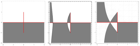
Figure 3.2. The sign of $\mathop{\rm Re}(i\theta)$ as $\xi$ increases from $-\infty$ to $+\infty$. Gray: $\mathop{\rm Re}(i\theta)<0$; White: $\mathop{\rm Re}(i\theta)>0$. Top row: $\xi=-\infty$, $\xi\in(-\infty,v_{o})$, $\xi=v_{o}$; Middle row: $\xi\in(v_{o},0)$, $\xi=0$, $\xi\in(0,-v_{o})$; Bottom row: $\xi=-v_{o}$, $\xi=(-v_{o},\infty)$, and $\xi=+\infty$.

Let us first focus on the sign structure of $\mathop{\rm Re}(i\theta)$ for $\xi<0$ (i.e. $x<0$), which is depicted in the first four frames of Figure 3.2. Observe that, as $\xi$ increases from $-\infty$ to $0$, the sign of $\mathop{\rm Re}(i\theta)$ switches from negative to positive in the third quadrant and from positive to negative in the second quadrant, while it remains the same in the first and the fourth quadrant. More specifically, two regions of positive sign emerge in the third quadrant: an unbounded region on the left of the point $k_{1}$, and a bounded region on the right of the point $k_{2}$ and on the left of the branch cut $B$, where

$$k_{1}(\xi):=\frac{1}{8}\left(\xi-\sqrt{\xi^{2}-v_{o}^{2}}\right),\quad k_{2}(\xi):=\frac{1}{8}\left(\xi+\sqrt{\xi^{2}-v_{o}^{2}}\right)$$ (3.17)

are the two stationary points of $\theta$ with $v_{o}$ defined by (2.10). The two regions of positive sign grow continuously and remain disjoint until $\xi=v_{o}$ (third frame in Figure 3.2) where $k_{1}(v_{o})=k_{2}(v_{o})=\frac{v_{o}}{8}$. Note that for $\xi\leqslant v_{o}$ the stationary points $k_{1},k_{2}$ are real. Subsequently, however, for $v_{o}<\xi<0$, the two stationary points become complex, and the two regions of positive sign merge to a single region that eventually grows to occupy all of the third quadrant (fourth and fifth frames in Figure 3.2). As a result, the value $\xi=v_{o}$ is a bifurcation point in the analysis of the problem via the Deift-Zhou method.

More specifically, for $\xi<v_{o}$, the sign structure of $\text{Re}(i\theta)$ allows for two different factorizations of the jump $V_{1}$ along the real axis, both of which result in exponentially decaying contributions, as will be explained in detail in Sections 4 and 5. On the other hand, for $v_{o}<\xi<0$ it turns out that only one of the aforementioned factorizations can be employed. This results in an exponentially growing jump along a certain portion of the deformed jump contour, which is corrected by introducing a so-called $g$-function [DVZ1, DVZ2] (see also Chapter 4 of [KMM] in the context of semiclassical analysis). The corresponding transformation of the Riemann-Hilbert problem replaces the original controlling phase function from $\theta$ to the Abelian integral $h$ defined by (2.5), and is the reason why the asymptotics change dramatically as $\xi$ crosses $v_{o}$. The sign structure of $\mathop{\rm Re}(ih)$ in the third quadrant of the complex $k$-plane as $\xi$ decreases from $v_{o}$ to 0 is shown in Figure 3.3.

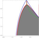
Figure 3.3. The sign of $\mathop{\rm Re}(ih)$ as $\xi$ increases gradually from $v_{o}$ (top left plot) to just below $\xi=0$ (bottom right plot). Gray: $\mathop{\rm Re}(ih)<0$; White: $\mathop{\rm Re}(ih)>0$. Note $h\equiv\theta$ when $\xi=v_{o}$. Red curves: The contours $\mathop{\rm Im}(h)=0$. Green curve: The path described by $\bar{\alpha}$ (defined by (2.8)), the intersection point of the contours $\mathop{\rm Im}(h)=0$. Black curve: The contour $\mathop{\rm Im}(\theta)=0$. Blue curve: The contour $\text{Im}\big{[}\theta(v_{o},k)\big{]}=0$.

Of course, apart from the jumps $V_{1}$, $V_{2}$, $V_{3}$ along the continuous spectrum, the Riemann-Hilbert problem (3.16) also involves the jumps $V_{p},V_{\bar{p}}$ originating from the poles $p,\bar{p}$. Thus, another crucial value of $\xi$ now emerges, namely the value $v_{s}$ for which $\text{Re}(i\theta)$ vanishes at $p$ and $\bar{p}$. Observe that $v_{s}$ is the same for $p$ and $\bar{p}$, since $\mathop{\rm Re}\left[i\theta(\xi,p)\right]=0\Leftrightarrow\mathop{\rm Re}\left[i\theta(\xi,\bar{p})\right]=0$ due to the symmetry $\theta(\xi,\bar{k})=\overline{\theta(\xi,k)}$. Solving either of these equations, we obtain $v_{s}$ in the explicit form (2.10). Note that in the third quadrant, where $p$ lies, we have $\lambda_{\textnormal{re}},\lambda_{\textnormal{im}}\leqslant 0$, thus $v_{s}<0$.

In the range $(-\infty,v_{o})$, we shall see that the jumps $V_{p},V_{\bar{p}}$ (equivalently, the poles $p,\bar{p}$) contribute to the leading-order asymptotics only when $\xi=v_{s}$, provided that $p$ is such that $v_{s}\in(-\infty,v_{o})$. On the other hand, as explained above, in the range $(v_{o},0)$ the phase function $\theta$ is replaced by the Abelian integral $h$ defined by (2.5). Thus, the role of $v_{s}$ is now played by the solutions of the equation

$$\mathop{\rm Re}\left[ih(\xi,p)\right]=0.$$ (3.18)

The complicated form of $h$ does not allow us to solve equation (3.18) explicitly. It turns out, however, that, depending on the location of $p$ inside the third quadrant, equation (3.18) has either zero, one or two solutions in the interval $(v_{o},0)$. More specifically, as already noted in Section 2, the third quadrant is divided into the four regions $D_{1}$, $D_{2}^{+}$, $D_{2}^{-}$, $D_{3}$ of Figure 2.1, where for $\xi\in(v_{o},0)$ equation (3.18) has no solutions in $D_{1}$, a unique solution $\widetilde{v}_{s}$ in $D_{2}^{+}$, two solutions $\widetilde{v}_{s}<v_{w}$ in $D_{2}^{-}$, and a unique solution $v_{w}$ in $D_{3}$. The mathematical description of the long-time asymptotic regimes that arise in these four regions is given in Theorems 2.1-2.4. Before proceeding to the proofs of these results, we give a brief outline of the way in which the asymptotics unravels in each regime. $p\in D_{1}$: The transmission regime. In this case, $v_{s}<v_{o}$ and, furthermore, equation (3.18) has no solution in the interval $(v_{o},0)$ — in fact, $\text{Re}(ih)(\xi,p)>0$ for all $v_{o}<\xi<0$. For $\xi<v_{s}$, the jumps $V_{p},V_{\bar{p}}$ decay exponentially and hence do not yield leading-order contributions. Thus, the dominant component of Riemann-Hilbert problem (3.16) in the limit $t\to\infty$ involves only the jumps along the continuous spectrum $\Sigma$, giving rise to the plane wave (2.14). At $\xi=v_{s}$, the jumps $V_{p},V_{\bar{p}}$ switch from exponentially decaying to purely oscillatory. Consequently, they are now part of the dominant Riemann-Hilbert problem, generating the soliton (2.16). Observe that this soliton propagates with velocity $v_{s}$ and, since $|v_{s}|>|v_{o}|$, it eventually escapes to infinity outside the wedge $|\xi|<|v_{o}|$ of Figure 2.2. For $v_{s}<\xi<v_{o}$, the jumps $V_{p},V_{\bar{p}}$ grow exponentially. Nevertheless, it turns out that this growth can be converted into decay via an appropriate transformation. Hence, similarly to the range $\xi<v_{s}$, the leading-order asymptotic behavior does not depend on $V_{p},V_{\bar{p}}$ and is characterized by the plane wave (2.14), but now with a phase shift generated by the soliton that has arisen at $\xi=v_{s}$. Finally, for $v_{o}<\xi<0$ the phase function switches from $\theta$ to $h$. Then, since $\text{Re}(ih)(\xi,p)>0$ for all $v_{o}<\xi<0$, the jumps $V_{p},V_{\bar{p}}$ do not contribute to the leading-order asymptotics. Hence, no soliton is present in the range $v_{o}<\xi<0$ and the solution is asymptotically equal to the modulated elliptic wave (2.20) with the phase shift already generated by the soliton at $\xi=v_{s}$ in the range $v_{s}<\xi<v_{o}$. $p\in D_{2}^{+}$: The trap regime. In this case, $v_{s}>v_{o}$ and, in addition, equation (3.18) has a unique solution $\widetilde{v}_{s}$ in the interval $(v_{o},0)$ — in fact, it turns out that $v_{s}<\widetilde{v}_{s}$. Thus, for $\xi<\widetilde{v}_{s}$ the jumps $V_{p},V_{\bar{p}}$ are not significant at leading order. In particular, for $\xi<v_{o}$ the leading-order asymptotics is given by the plane wave (2.14), while for $v_{o}<\xi<\widetilde{v}_{s}$ the solution is asymptotically equal to the modulated elliptic wave (2.22). At $\xi=\widetilde{v}_{s}$, however, the jumps $V_{p},V_{\bar{p}}$ become purely oscillatory and hence do contribute to the leading-order asymptotics, which is now given by the soliton (2.23). Observe that, since $|\widetilde{v}_{s}|<|v_{o}|$, this soliton is trapped forever inside the wedge $|\xi|<|v_{o}|$ of Figure 2.2. Furthermore, the fact that $|\widetilde{v}_{s}|<|v_{s}|$ indicates that the soliton is delayed by its interaction with the modulated elliptic wave. Finally, since $\widetilde{v}_{s}$ is the only solution of equation (3.18) in $(v_{o},0)$, for $\widetilde{v}_{s}<\xi<0$ the jumps $V_{p},V_{\bar{p}}$ do not affect the leading-order asymptotics, which is now equal to the modulated elliptic wave (2.20) with an additional phase shift generated by the soliton at $\xi=\widetilde{v}_{s}$. $p\in D_{2}^{-}$: The trap/wake regime. This case is similar to the trap regime apart from the fact that now equation (3.18) has two (as opposed to one) solutions in the interval $(v_{o},0)$, namely $\widetilde{v}_{s}$ and $v_{w}$ with $\widetilde{v}_{s}<v_{w}$. Therefore, for $\xi<v_{w}$ the asymptotics is the same with the one in the trap regime, including the soliton that arises at $\xi=\widetilde{v}_{s}$. However, at $\xi=v_{w}$ a new phenomenon emerges, namely the soliton wake (2.25). Importantly, contrary to the soliton (which induces a phase shift for $\xi>\widetilde{v}_{s}$), the soliton wake does not affect the leading-order asymptotics in the range $v_{w}<\xi<0$. $p\in D_{3}$: The transmission/wake regime. This case is similar to the transmission regime apart from the fact that equation (3.18) now has a unique solution $v_{w}$ in the interval $(v_{o},0)$ (as opposed to no solution). Thus, the leading-order asymptotics is the same with the one in the transmission regime except for $\xi=v_{w}$, where the soliton wake (2.25) arises. Importantly, contrary to the soliton at $\xi=v_{s}$ (which generates a phase shift for $\xi>v_{s}$), the leading-order asymptotics for $v_{w}<\xi<0$ are not affected by the soliton wake.

4. The Transmission Regime: Proof of Theorem 2.1

This regime arises when $p$ lies in the region $D_{1}$ of Figure 2.1, in which case $v_{s}<v_{o}$ and $\text{Re}(ih)(\xi,p)$ does not vanish in the interval $(v_{o},0)$. Thus, we split the interval $(-\infty,0)$ into the following ranges: $\xi<v_{s}$; $\xi=v_{s}$; $v_{s}<\xi<v_{o}$; and $v_{o}<\xi<0$.

4.1. The range $\xi<v_{s}$: plane wave

In this range, we have $\mathop{\rm Re}(i\theta)(\xi,p)<0$ and $\mathop{\rm Re}(i\theta)(\xi,\bar{p})>0$. Hence, the jumps $V_{p}$ and $V_{\bar{p}}$ given by (3.15) tend to the identity as $t\to\infty$ and therefore are not expected to be part of the dominant component of Riemann-Hilbert problem (3.16) in the limit $t\to\infty$. Next, we shall show that this is indeed the case by performing several deformations of problem (3.16) in the spirit of the Deift-Zhou nonlinear steepest descent method. We emphasize that although some of these deformations are similar to those of the no-discrete-spectrum analysis of [BM2], one now needs to carefully handle the jumps around the poles $p$, $\bar{p}$, which were not present in [BM2]. First deformation. This deformation is carried out in four stages. In each of these stages, a new function $N^{(1)}$ is defined in terms of the solution $N=N^{(0)}$ of Riemann-Hilbert problem (3.16), as shown in Figures 4.2-4.4. Importantly, the jumps $V_{p}=V_{p}^{(0)}$ and $V_{\bar{p}}=V_{\bar{p}}^{(0)}$ are not affected by this deformation. In its final form, the function $N^{(1)}$ is analytic in $\mathbb{C}\setminus\big{(}\bigcup_{j=0}^{4}L_{j}\cup B\cup\partial D_{p}^{\varepsilon}\cup\partial D_{\bar{p}}^{\varepsilon}\big{)}$, satisfies the asymptotic condition

$$N^{(1)}=I+O\left(\frac{1}{k}\right),\quad k\to\infty,$$ (4.1)

and possesses the following jump discontinuities along the contours $\bigcup_{j=0}^{4}L_{j}\cup B\cup\partial D_{p}^{\varepsilon}\cup\partial D_{\bar{p}}^{\varepsilon}$, as shown in Figure 4.4:

$$V_{B}^{(1)}=V_{B}=\left(\begin{array}[]{lr}0&\tfrac{q_{-}}{iq_{o}}\\ \tfrac{\bar{q}_{-}}{iq_{o}}&0\end{array}\right),\quad V_{0}^{(1)}=\left(\begin{array}[]{lr}1+r\bar{r}&0\\ 0&\dfrac{1}{1+r\bar{r}}\end{array}\right),\quad V_{1}^{(1)}=\left(\begin{array}[]{lr}d^{-\frac{1}{2}}&\dfrac{d^{\frac{1}{2}}\,\bar{r}e^{2i\theta t}}{1+r\bar{r}}\\ 0&d^{\frac{1}{2}}\end{array}\right),$$ (4.8)

$$V_{2}^{(1)}=\left(\begin{array}[]{lr}d^{-\frac{1}{2}}&0\\ \dfrac{d^{\frac{1}{2}}re^{-2i\theta t}}{1+r\bar{r}}&d^{\frac{1}{2}}\end{array}\right),\quad V_{3}^{(1)}=\left(\begin{array}[]{lr}d^{-\frac{1}{2}}&0\\ d^{-\frac{1}{2}}re^{-2i\theta t}&d^{\frac{1}{2}}\end{array}\right),\quad V_{4}^{(1)}=\left(\begin{array}[]{lr}d^{-\frac{1}{2}}&d^{-\frac{1}{2}}\bar{r}e^{2i\theta t}\\ 0&d^{\frac{1}{2}}\end{array}\right),$$ (4.15)

$$\hskip 150.79968ptV_{p}^{(1)}=V_{p}^{(0)},\quad V_{\bar{p}}^{(1)}=V_{\bar{p}}^{(0)}.$$ (4.16)

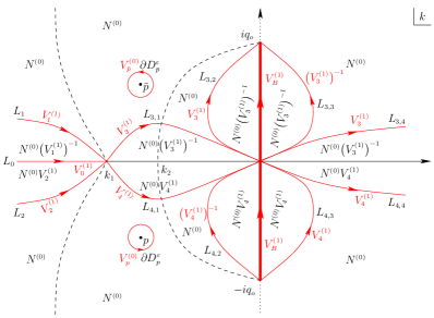
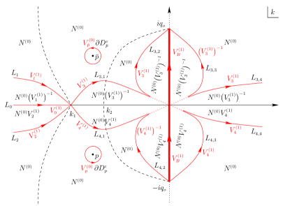
Figure 4.1. Plane wave region in the transmission regime: the first stage of the first deformation. A new function $N^{(1)}$ is defined in terms of the solution $N^{(0)}$ of Riemann-Hilbert problem (3.16) via different expressions in different regions of the complex $k$-plane. This allows us to eliminate the jump of (3.16) along $(k_{1},\infty)$. The jumps $V_{p}=V_{p}^{(0)}$ and $V_{\bar{p}}=V_{\bar{p}}^{(0)}$ along the circles $\partial D_{p}^{\varepsilon}$ and $\partial D_{\bar{p}}^{\varepsilon}$ are not affected at this stage.

Figure 4.2. Plane wave region in the transmission regime: the second stage of the first deformation. In the second quadrant, the function $N^{(1)}$ is defined in terms of $N^{(0)}$ by the same expression both below the contour $L_{3,1}$ and to the right of the contour $L_{3,2}$. Thus, $N^{(1)}$ does not have a jump along the overlapping portion between these two contours (dotted line), allowing one to lift them away from the origin. The same is true for the contour pairs $\{L_{3,3},L_{3,4}\}$, $\{L_{4,1},L_{4,2}\}$ and $\{L_{4,3},L_{4,4}\}$. The jumps along $\partial D_{p}^{\varepsilon}$ and $\partial D_{\bar{p}}^{\varepsilon}$ remain unchanged.

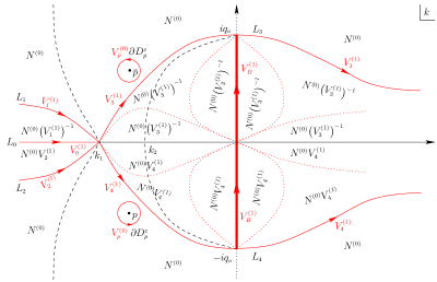
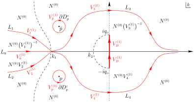
Figure 4.3. Plane wave region in the transmission regime: the third stage of the first deformation. Having lifted the jump contours away from the origin as shown in Figure 4.2, one can now adjust the definition of $N^{(1)}$ according to the present figure in order to move these jump contours outside the finite region defined by the branch cut $B$ and the dashed line through the stationary point $k_{2}$. This ensures that the relevant jumps occur along contours of appropriate sign for $\text{Re}(i\theta)$. The jumps along $\partial D_{p}^{\varepsilon}$ and $\partial D_{\bar{p}}^{\varepsilon}$ are as before.

Figure 4.4. Plane wave region in the transmission regime: the fourth and final stage of the first deformation. The jump contours $L_{3}$ and $L_{4}$ have been lifted away from the branch points $\pm iq_{o}$ similarly to [BM2]. Overall, the jumps along $\partial D_{p}^{\varepsilon}$ and $\partial D_{\bar{p}}^{\varepsilon}$ have not changed in the transition from $N^{(0)}$ to $N^{(1)}$, i.e. $V_{p}^{(1)}=V_{p}^{(0)}$ and $V_{\bar{p}}^{(1)}=V_{\bar{p}}^{(0)}$.

Second deformation. The jump $V_{0}^{(1)}$ along the contour $L_{0}:=(-\infty,k_{1})$ shown in Figure 4.4 can be removed by means of the transformation

$$N^{(2)}(x,t,k)=N^{(1)}(x,t,k)\delta(\xi,k)^{-\sigma_{3}},$$ (4.17)

where the scalar function $\delta(\xi,k)$ is analytic in $\mathbb{C}\setminus(-\infty,k_{1})$ and satisfies the Riemann-Hilbert problem

$$\delta^{+} =\delta^{-}\left(1+r\bar{r}\right),\quad k\in(-\infty,k_{1}),$$ (4.18a)

$$\delta =1+O\left(\tfrac{1}{k}\right), k\to\infty.$$ (4.18b)

In fact, problem (4.18) can be solved explicitly via the Plemelj formulae to yield

$$\delta(\xi,k)=\exp\left\{\frac{1}{2i\pi}\int_{-\infty}^{k_{1}(\xi)}\frac{\ln\left[1+r(\nu)\bar{r}(\nu)\right]}{\nu-k}\,d\nu\right\},\quad k\notin(-\infty,k_{1}).$$ (4.19)

Through transformation (4.17), the jumps of $N^{(1)}$ give rise to corresponding jumps for $N^{(2)}$. As shown in Figure 4.6, these jumps occur along the contours $\bigcup_{j=1}^{4}L_{j}\cup B$ and are given by

$$V_{B}^{(2)}=\left(\begin{array}[]{lr}0&\tfrac{q_{-}}{iq_{o}}\delta^{2}\\ \tfrac{\bar{q}_{-}}{iq_{o}}\delta^{-2}&0\end{array}\right),\quad V_{1}^{(2)}=\left(\begin{array}[]{lr}d^{-\frac{1}{2}}&\dfrac{d^{\frac{1}{2}}\,\bar{r}e^{2i\theta t}}{1+r\bar{r}}\delta^{2}\\ 0&d^{\frac{1}{2}}\end{array}\right),\quad V_{2}^{(2)}=\left(\begin{array}[]{lr}d^{-\frac{1}{2}}&0\\ \dfrac{d^{\frac{1}{2}}re^{-2i\theta t}}{1+r\bar{r}}\delta^{-2}&d^{\frac{1}{2}}\end{array}\right),$$ (4.26)

$$\hskip 56.9055ptV_{3}^{(2)}=\left(\begin{array}[]{lr}d^{-\frac{1}{2}}&0\\ d^{-\frac{1}{2}}re^{-2i\theta t}\delta^{-2}&d^{\frac{1}{2}}\end{array}\right),\quad V_{4}^{(2)}=\left(\begin{array}[]{lr}d^{-\frac{1}{2}}&d^{-\frac{1}{2}}\bar{r}e^{2i\theta t}\delta^{2}\\ 0&d^{\frac{1}{2}}\end{array}\right),$$ (4.31)

as well as along the disks $\partial D_{p}^{\varepsilon}$ and $\partial D_{\bar{p}}^{\varepsilon}$, where they read (modified for the first time)

$$V_{p}^{(2)}=\left(\begin{array}[]{lr}1&-\dfrac{c_{p}\,\delta^{2}(\xi,k)}{k-p}\,e^{2i\theta(\xi,p)t}\\ 0&1\end{array}\right),\quad V_{\bar{p}}^{(2)}=\left(\begin{array}[]{lr}1&0\\ -\dfrac{c_{\bar{p}}\,\delta^{-2}(\xi,k)}{k-\bar{p}}\,e^{-2i\theta(\xi,\bar{p})t}&1\end{array}\right).$$ (4.32)

Finally, the normalization condition (4.19) for $N^{(1)}$ is also satisfied by $N^{(2)}$.

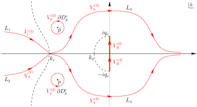
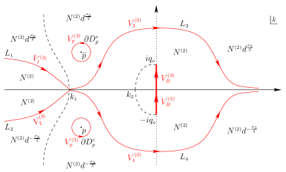
Figure 4.5. Plane wave region in the transmission regime: the second deformation.

Figure 4.6. Plane wave region in the transmission regime: the third deformation.

Third deformation. The function $d(k)$ can be eliminated from the jump matrices along $\bigcup_{j=1}^{4}L_{j}$ by introducing a new function $N^{(3)}$ defined in terms of $N^{(2)}$ according to Figure 4.6. In particular, the jumps of $N^{(3)}$ along the contours $\bigcup_{j=1}^{4}L_{j}\cup B$ are given by

$$V_{B}^{(3)}=\left(\begin{array}[]{lr}0&\tfrac{q_{-}}{iq_{o}}\delta^{2}\\ \tfrac{\bar{q}_{-}}{iq_{o}}\delta^{-2}&0\end{array}\right),\quad V_{1}^{(3)}=\left(\begin{array}[]{lr}1&\dfrac{\bar{r}e^{2i\theta t}}{1+r\bar{r}}\delta^{2}\\ 0&1\end{array}\right),\quad V_{2}^{(3)}=\left(\begin{array}[]{lr}1&0\\ \dfrac{re^{-2i\theta t}}{1+r\bar{r}}\delta^{-2}&1\end{array}\right),$$ (4.39)

$$\hskip 76.82234ptV_{3}^{(3)}=\left(\begin{array}[]{lr}1&0\\ re^{-2i\theta t}\delta^{-2}&1\end{array}\right),\quad V_{4}^{(3)}=\left(\begin{array}[]{lr}1&\bar{r}e^{2i\theta t}\delta^{2}\\ 0&1\end{array}\right).$$ (4.44)

Moreover, noting that $N^{(3)}=N^{(2)}d^{-\frac{\sigma_{3}}{2}}$ for $k\in D_{p}^{\varepsilon}$ and $N^{(3)}=N^{(2)}d^{\frac{\sigma_{3}}{2}}$ for $k\in D_{\bar{p}}^{\varepsilon}$, we obtain

$$V_{p}^{(3)}=\left(\begin{array}[]{lr}1&-\dfrac{c_{p}\,\delta^{2}(\xi,k)\,d(k)}{k-p}\,e^{2i\theta(\xi,p)t}\\ 0&1\end{array}\right),\ V_{\bar{p}}^{(3)}=\left(\begin{array}[]{lr}1&0\\ -\dfrac{c_{\bar{p}}\,\delta^{-2}(\xi,k)\,d(k)}{k-\bar{p}}\,e^{-2i\theta(\xi,\bar{p})t}&1\end{array}\right).$$ (4.45)

Fourth deformation. Our final goal is to convert the jump along the branch cut $B$ into the constant matrix $V_{B}$ given by (4.8). This can be achieved by means of the global transformation

$$N^{(4)}(x,t,k)=N^{(3)}(x,t,k)e^{ig(\xi,k)\sigma_{3}},$$ (4.46)

where the function $g(\xi,k)$ is analytic in $\mathbb{C}\setminus B$ and satisfies the jump condition

$$e^{i(g^{+}+g^{-})}=\delta^{2},\quad k\in B,$$ (4.47)

and the normalization condition

$$\frac{g}{\lambda}=O\left(\frac{1}{k}\right),\quad k\to\infty.$$ (4.48)

Indeed, the jump condition (4.47) implies that the jump of $N^{(4)}$ along $B$ is precisely $V_{B}$. Equations (4.47) and (4.48) formulate a Riemann-Hilbert problem for $g$, which can be solved explicitly to yield

$$g(\xi,k)=\frac{\lambda(k)}{2i\pi^{2}}\int_{\zeta\in B}\frac{1}{\lambda(\zeta)\left(\zeta-k\right)}\int_{-\infty}^{k_{1}(\xi)}\frac{\ln\left[1+r(\nu)\bar{r}(\nu)\right]}{\nu-\zeta}\,d\nu d\zeta,\quad k\notin B.$$ (4.49)

Under transformation (4.46), the Riemann-Hilbert problem for $N^{(3)}$ turns into the following Riemann-Hilbert problem for $N^{(4)}$:

$$N^{(4)+} =N^{(4)-}V_{B}, k\in B,$$ (4.50a)

$$N^{(4)+} =N^{(4)-}V_{j}^{(4)}, k\in L_{j},\ j=1,2,3,4,$$ (4.50b)

$$N^{(4)+} =N^{(4)-}V_{p}^{(4)}, k\in\partial D_{p}^{\varepsilon},$$ (4.50c)

$$N^{(4)+} =N^{(4)-}V_{\bar{p}}^{(4)}, k\in\partial D_{\bar{p}}^{\varepsilon},$$ (4.50d)

$$N^{(4)} =\left[I+O\left(\tfrac{1}{k}\right)\right]e^{ig_{\infty}(\xi)\sigma_{3}},\quad k\to\infty,$$ (4.50e)

with the jump $V_{B}$ given by (4.8) and

$$V_{1}^{(4)}=\left(\begin{array}[]{lr}1&\dfrac{\bar{r}e^{2i(\theta t-g)}}{1+r\bar{r}}\,\delta^{2}\\ 0&1\end{array}\right),\quad V_{2}^{(4)}=\left(\begin{array}[]{lr}1&0\\ \dfrac{re^{-2i(\theta t-g)}}{1+r\bar{r}}\,\delta^{-2}&1\end{array}\right),\quad V_{3}^{(4)}=\left(\begin{array}[]{lr}1&0\\ re^{-2i(\theta t-g)}\delta^{-2}&1\end{array}\right),$$ (4.57)

$$V_{4}^{(4)}=\left(\begin{array}[]{lr}1&\bar{r}e^{2i(\theta t-g)}\delta^{2}\\ 0&1\end{array}\right),\quad V_{p}^{(4)}=\left(\begin{array}[]{lr}1&-\dfrac{c_{p}\,\delta^{2}(\xi,k)\,d(k)\,e^{-2ig(\xi,k)}}{k-p}\,e^{2i\theta(\xi,p)t}\\ 0&1\end{array}\right),$$ (4.62)

$$V_{\bar{p}}^{(4)}=\left(\begin{array}[]{lr}1&0\\ -\dfrac{c_{\bar{p}}\,\delta^{-2}(\xi,k)\,d(k)\,e^{2ig(\xi,k)}}{k-\bar{p}}\,e^{-2i\theta(\xi,\bar{p})t}&1\end{array}\right),$$ (4.65)

where the associated jump contours are shown in Figure 4.6 and $g_{\infty}(\xi)$ is the limit of $g(\xi,k)$ as $k\to\infty$, i.e.

$$g_{\infty}(\xi):=\lim_{k\to\infty}g(\xi,k)=-\frac{1}{2i\pi^{2}}\int_{\zeta\in B}\frac{1}{\lambda(\zeta)}\int_{-\infty}^{k_{1}(\xi)}\frac{\ln\left[1+r(\nu)\bar{r}(\nu)\right]}{\nu-\zeta}\,d\nu d\zeta.$$ (4.66)

Importantly, expressing $g_{\infty}$ in terms of $\delta$ and using the symmetries $\overline{\lambda(k)}=\lambda(\bar{k})$ and $\overline{\delta(\xi,k)}=\left[\delta(\xi,\bar{k})\right]^{-1}$, we have that $\overline{g_{\infty}(\xi)}=g_{\infty}(\xi)$, i.e. that $g_{\infty}\in\mathbb{R}$.

Observe that all the jumps of $N^{(4)}$ apart from $V_{B}$ tend to the identity exponentially fast in the limit $t\to\infty$. Hence, proceeding as in the appendix of [BM2], we find that the contribution of these jumps is of order $O(t^{-1/2})$. Then, starting from the reconstruction formula (3.13) and applying the four successive deformations that lead to $N^{(4)}$, we eventually obtain

$$q(x,t)=-2i\lim_{k\to\infty}\left[kN_{12}^{\textnormal{dom}}(x,t,k)\right]e^{ig_{\infty}(\xi)}+O\big{(}t^{-\frac{1}{2}}\big{)},\quad t\to\infty,$$ (4.67)

where $N^{\textnormal{dom}}(x,t,k)$ satisfies the dominant component of Riemann-Hilbert problem (4.50), that is

$$N^{{\textnormal{dom}}+} =N^{{\textnormal{dom}}-}V_{B}, k\in B,$$ (4.68a)

$$N^{\textnormal{dom}} =\left[I+O\left(\tfrac{1}{k}\right)\right]e^{ig_{\infty}(\xi)\sigma_{3}},\quad k\to\infty.$$ (4.68b)

The dominant problem (4.68) has been extracted from problem (4.50) in a similar way with problem (4.73) of Subsection 4.2. In fact, it is straightforward to verify that $N^{\textnormal{dom}}$ is given by the explicit formula

$$N^{\textnormal{dom}}=\frac{1}{2}\,e^{ig_{\infty}(\xi)\sigma_{3}}\left(\begin{array}[]{lr}\Lambda(k)+\Lambda^{-1}(k)&-\dfrac{q_{o}}{\bar{q}_{-}}\left[\Lambda(k)-\Lambda^{-1}(k)\right]\\ -\dfrac{q_{o}}{q_{-}}\left[\Lambda(k)-\Lambda^{-1}(k)\right]&\Lambda(k)+\Lambda^{-1}(k)\end{array}\right),$$ (4.69)

where

$$\Lambda(k):=\left(\frac{k-iq_{o}}{k+iq_{o}}\right)^{\frac{1}{4}}.$$ (4.70)

Expressions (4.67) and (4.69) yield the leading-order asymptotics (2.14) in the range $\xi<v_{s}$ of the transmission regime $p\in D_{1}$. We note that, as expected from the fact that the discrete spectrum does not contribute at leading order for $\xi<v_{s}$, (2.14) is consistent with the result obtained for $\xi<v_{o}$ in the case of no discrete spectrum analyzed in [BM2].

4.2. The case $\xi=v_{s}$: soliton on top of a plane wave

The same four deformations that were performed for $\xi<v_{s}$ yield once again Riemann-Hilbert problem (4.50). In particular, the jumps along $\partial D_{p}^{\varepsilon}$ and $\partial D_{\bar{p}}^{\varepsilon}$ read

$$V_{p}^{(4)} =\left(\begin{array}[]{lr}1&-\dfrac{c_{p}\,\delta^{2}(v_{s},k)\,d(k)\,e^{-2ig(v_{s},k)}}{k-p}\,e^{2i\theta(v_{s},p)t}\\ 0&1\end{array}\right),$$ (4.71c)

$$V_{\bar{p}}^{(4)} =\left(\begin{array}[]{lr}1&0\\ -\dfrac{c_{\bar{p}}\,\delta^{-2}(v_{s},k)\,d(k)\,e^{2ig(v_{s},k)}}{k-\bar{p}}\,e^{-2i\theta(v_{s},\bar{p})t}&1\end{array}\right).$$ (4.71f)

However, since $\mathop{\rm Re}(i\theta)(v_{s},p)=\mathop{\rm Re}(i\theta)(v_{s},\bar{p})=0$, the time-dependent exponentials involved in the jumps (4.71) are purely oscillatory (as opposed to decaying). That is, contrary to the range $\xi<v_{s}$, the jumps $V_{p}^{(4)}$ and $V_{\bar{p}}^{(4)}$ no longer tend to the identity as $t\to\infty$. Hence, $V_{p}^{(4)}$ and $V_{\bar{p}}^{(4)}$ are now expected to contribute to the leading-order asymptotics (together, of course, with the jump $V_{B}$ along the branch cut $B$, which is constant) and, therefore, they must be included in the dominant component of problem (4.50). Next, we extract the dominant component from the rest of the problem.

Decomposition into dominant and error problems. Let $D_{k_{1}}^{\epsilon}$ be a disk centered at $k_{1}$ with radius $\epsilon$ sufficiently small so that $D_{k_{1}}^{\epsilon}\cap\left(B\cup\overline{D_{p}^{\varepsilon}\cup D_{\bar{p}}^{\varepsilon}}\right)=\O$. Then, write the solution $N^{(4)}$ of problem (4.50) in the form

$$N^{(4)}=N^{\textnormal{err}}N^{\textnormal{asymp}},\quad N^{\textnormal{asymp}}=\begin{cases}N^{\textnormal{dom}},&k\in\mathbb{C}\setminus D_{k_{1}}^{\epsilon},\\ N^{k_{1}},&k\in D_{k_{1}}^{\epsilon},\end{cases}$$ (4.72)

where the components $N^{\textnormal{dom}}$, $N^{k_{1}}$ and $N^{\textnormal{err}}$ are defined as follows:

1. The function $N^{\textnormal{dom}}(v_{s}t,t,k)$ is analytic in $\mathbb{C}\setminus\left(B\cup\partial D_{p}^{\varepsilon}\cup\partial D_{\bar{p}}^{\varepsilon}\right)$ and satisfies the Riemann-Hilbert problem

   $$N^{{\textnormal{dom}}+} =N^{{\textnormal{dom}}-}V_{B}, k\in B,$$ (4.73a)

   $$N^{{\textnormal{dom}}+} =N^{{\textnormal{dom}}-}V_{p}^{(4)}, k\in\partial D_{p}^{\varepsilon},$$ (4.73b)

   $$N^{{\textnormal{dom}}+} =N^{{\textnormal{dom}}-}V_{\bar{p}}^{(4)}, k\in\partial D_{\bar{p}}^{\varepsilon},$$ (4.73c)

   $$N^{\textnormal{dom}} =\left[I+O\left(\tfrac{1}{k}\right)\right]e^{ig_{\infty}(v_{s})\sigma_{3}},\quad k\to\infty,$$ (4.73d)

   with $V_{B}$ given by (4.8) and $V_{p}^{(4)}$, $V_{\bar{p}}^{(4)}$ given by (4.71).

2. The function $N^{k_{1}}(v_{s}t,t,k)$ is analytic in $D_{k_{1}}^{\epsilon}\setminus\bigcup_{j=1}^{4}L_{j}$ with jumps

   $$N^{k_{1}+}=N^{k_{1}-}V_{j}^{(4)},\quad k\in\widehat{L}_{j}:=L_{j}\cap D_{k_{1}}^{\epsilon},\ j=1,2,3,4.$$ (4.74)

   Note that nothing has been specified about $N^{k_{1}}$ outside the disk $D_{k_{1}}^{\epsilon}$.

3. The function $N^{\textnormal{err}}(v_{s},t,k)$ is analytic in $\mathbb{C}\setminus\big{(}\bigcup_{j=1}^{4}\savestack{\tmpbox}{\stretchto{\scaleto{\scalerel*[width("L")]{\kern-0.6pt\bigwedge\kern-0.6pt}{\rule[-505.89pt]{4.30554pt}{505.89pt}}}{}}{0.5ex}}\stackon[1pt]{L}{\scalebox{-1.0}{\tmpbox}}_{j}\cup\partial D_{k_{1}}^{\epsilon}\big{)}$, where $\savestack{\tmpbox}{\stretchto{\scaleto{\scalerel*[width("L")]{\kern-0.6pt\bigwedge\kern-0.6pt}{\rule[-505.89pt]{4.30554pt}{505.89pt}}}{}}{0.5ex}}\stackon[1pt]{L}{\scalebox{-1.0}{\tmpbox}}_{j}:=L_{j}\setminus\widehat{L}_{j}$, and satisfies the Riemann-Hilbert problem

   $$N^{{\textnormal{err}}+} =N^{{\textnormal{err}}-}V^{\textnormal{err}},\quad$$

   $$N^{\textnormal{err}} =I+O\left(\tfrac{1}{k}\right), k\to\infty,$$ (4.75a)

   where

   $$V^{\textnormal{err}}=\begin{cases}N^{\textnormal{dom}}V_{j}^{(4)}(N^{\textnormal{dom}})^{-1},&k\in\savestack{\tmpbox}{\stretchto{\scaleto{\scalerel*[width("L")]{\kern-0.6pt\bigwedge\kern-0.6pt}{\rule[-505.89pt]{4.30554pt}{505.89pt}}}{}}{0.5ex}}\stackon[1pt]{L}{\scalebox{-1.0}{\tmpbox}}_{j},\\ N^{{\textnormal{asymp}}-}(V_{D}^{\textnormal{asymp}})^{-1}(N^{{\textnormal{asymp}}-})^{-1},&k\in\partial D_{k_{1}}^{\epsilon},\end{cases}$$ (4.75bx)

   and $V_{D}^{\textnormal{asymp}}$ is the yet unknown jump of $N^{\textnormal{asymp}}$ along the circle $\partial D_{k_{1}}^{\epsilon}$.

   Under the four successive deformations that lead to problem (4.50), the reconstruction formula (3.13) becomes

   $$q(x,t)=-2i\lim_{k\to\infty}kN_{12}^{(4)}(v_{s}t,t,k)e^{ig_{\infty}(v_{s})},$$ (4.75by)

   where we have also used the fact that $\delta,d\to 1$ as $k\to\infty$. This formula combined with the decomposition (4.72) and the asymptotic conditions (4.73d) and (4.75a) implies

   $$q(x,t)=-2i\lim_{k\to\infty}k\left[N_{12}^{\textnormal{dom}}(v_{s}t,t,k)e^{ig_{\infty}(v_{s})}+N_{12}^{\textnormal{err}}(v_{s}t,t,k)\right].$$ (4.75bz)

   The error problem (4.75) is precisely that of the plane wave region in [BM2], since the jumps around $p$ and $\bar{p}$ are not part of this problem. Hence, as shown in [BM2], $\lim_{k\to\infty}kN_{12}^{\textnormal{err}}=O\big{(}t^{-1/2}\big{)}$. In turn, we obtain

   $$q(x,t)=-2i\lim_{k\to\infty}kN_{12}^{\textnormal{dom}}(v_{s}t,t,k)e^{ig_{\infty}(v_{s})}+O\big{(}t^{-\frac{1}{2}}\big{)},\quad t\to\infty.$$ (4.75ca)

   It remains to determine $N^{\textnormal{dom}}$, i.e. to solve the dominant Riemann-Hilbert problem (4.73).

   Solution of the dominant problem. We begin by converting the jumps along the circles $\partial D_{p}^{\varepsilon}$ and $\partial D_{\bar{p}}^{\varepsilon}$ back to residue conditions at $p$ and $\bar{p}$. This is done by reverting transformation (3.14), i.e. by letting

   $$M^{\textnormal{dom}}=\left\{\begin{array}[]{ll}N^{\textnormal{dom}}\big{(}V_{p}^{(4)}\big{)}^{-1},&k\in D_{p}^{\varepsilon},\\ N^{\textnormal{dom}},&k\in\mathbb{C}^{-}\setminus\left(B^{-}\cup\overline{D_{p}^{\varepsilon}}\,\right),\\ N^{\textnormal{dom}}\big{(}V_{\bar{p}}^{(4)}\big{)}^{-1},&k\in D_{\bar{p}}^{\varepsilon},\\ N^{\textnormal{dom}},&k\in\mathbb{C}^{+}\setminus\left(B^{+}\cup\overline{D_{\bar{p}}^{\varepsilon}}\,\right).\end{array}\right.$$ (4.75cb)

   Then, $M^{\textnormal{dom}}$ is the solution of the Riemann-Hilbert problem

   $$M^{{\textnormal{dom}}+} =M^{{\textnormal{dom}}-}V_{B}, k\in B,$$ (4.75cca)

   $$M^{\textnormal{dom}} =\left[I+O\left(\tfrac{1}{k}\right)\right]e^{ig_{\infty}(v_{s})\sigma_{3}},\quad k\to\infty,$$ (4.75ccb)

   $$\underset{k=p}{\text{Res}}\,M^{\textnormal{dom}} =\left(0,\rho_{p}\,M_{1}^{\textnormal{dom}}(p)\right),$$ (4.75ccc)

   $$\underset{k=\bar{p}}{\text{Res}}\,M^{\textnormal{dom}} =\left(\rho_{\bar{p}}\,M_{2}^{\textnormal{dom}}(\bar{p}),0\right),$$ (4.75ccd)

   where $M_{1}^{\textnormal{dom}},M_{2}^{\textnormal{dom}}$ denote the two columns of $M^{\textnormal{dom}}$ and

   $$\rho_{p}=c_{p}\delta^{2}(v_{s},p)d(p)e^{2i\left[\theta(v_{s},p)t-g(v_{s},p)\right]},$$ (4.75cda)

   $$\rho_{\bar{p}}=c_{\bar{p}}\delta^{-2}(v_{s},\bar{p})d(\bar{p})e^{-2i\left[\theta(v_{s},\bar{p})t-g(v_{s},\bar{p})\right]}.$$ (4.75cdb)

   In fact, the expressions for $\rho_{p}$ and $\rho_{\bar{p}}$ can be simplified after noting that the symmetry (see [BM2])

   $$\overline{\Psi_{\pm}(x,t,\bar{k})}=-\sigma_{*}\Psi_{\pm}(x,t,k)\sigma_{*},\quad\sigma_{*}:=\begin{pmatrix}0&1\\ -1&0\end{pmatrix},$$

   together with relations (3.10a) and (3.10b) imply $C_{\bar{p}}=-\overline{C_{p}}$. Then, recalling the Schwarz symmetries $\bar{a}^{\prime}(\bar{k})=\overline{a^{\prime}(k)}$, $d(\bar{k})=\overline{d(k)}$ and the definitions (3.11a) and (3.11b) of $c_{p}$ and $c_{\bar{p}}$, we obtain

   $$c_{\bar{p}}=-\overline{c_{p}}.$$ (4.75ce)

   Hence, noting in addition that $\theta(\xi,\bar{k})=\overline{\theta(\xi,k)}$, $g(\xi,\bar{k})=\overline{g(\xi,k)}$, $\delta(\xi,\bar{k})=\overline{\delta^{-1}(\xi,k)}$, and since $\theta(v_{s},\bar{p})\in\mathbb{R}$, we have

   $$\rho_{p}=R_{p}\,e^{2i\theta(v_{s},p)t},\quad\rho_{\bar{p}}=-\overline{R_{p}}\,e^{-2i\theta(v_{s},p)t},\quad R_{p}:=C_{p}\frac{\delta^{2}(v_{s},p)e^{-2ig(v_{s},p)}}{a^{\prime}(p)},$$ (4.75cf)

   which shows that $\rho_{\bar{p}}=-\overline{\rho_{p}}$.

   We will solve problem (4.75cc) by decomposing it into discrete and continuous spectrum components via the substitution

   $$M^{\textnormal{dom}}=\mathcal{M}^{\textnormal{dom}}W.$$ (4.75cg)

   Here, $W$ is the solution of the continuous spectrum component problem

   $$W^{+} =W^{-}V_{B}, k\in B,$$ (4.75cha)

   $$W =\left[I+O\left(\tfrac{1}{k}\right)\right]e^{ig_{\infty}(v_{s})\sigma_{3}},\quad k\to\infty,$$ (4.75chb)

   which is nothing but problem (4.68) evaluated at $\xi=v_{s}$. Therefore,

   $$W=\frac{1}{2}\,e^{ig_{\infty}(v_{s})\sigma_{3}}\left(\begin{array}[]{lr}\Lambda(k)+\Lambda^{-1}(k)&-\frac{q_{o}}{\bar{q}_{-}}\left[\Lambda(k)-\Lambda^{-1}(k)\right]\\ -\frac{q_{o}}{q_{-}}\left[\Lambda(k)-\Lambda^{-1}(k)\right]&\Lambda(k)+\Lambda^{-1}(k)\end{array}\right)$$ (4.75ci)

   with $\Lambda$ given by (4.70).

   Since $\det W\equiv 1\neq 0$, we can rearrange (4.75cg) to

   $$\mathcal{M}^{\textnormal{dom}}=M^{\textnormal{dom}}W^{-1}$$ (4.75cj)

   and hence deduce that $\mathcal{M}^{\textnormal{dom}}$ does not have a jump along $B$, i.e. $\mathcal{M}^{\textnormal{dom}}$ is indeed the discrete spectrum component of $M^{\textnormal{dom}}$. Moreover, since $M_{1}^{\textnormal{dom}}$ and $W$ are analytic at $p$, formula (4.75cj) and the residue condition (4.75ccc) imply

   $$\underset{k=p}{\text{Res}}\,\mathcal{M}_{1}^{\textnormal{dom}}=-W_{21}(p)\rho_{p}\,M_{1}^{\textnormal{dom}}(p).$$ (4.75cka)

   Similarly, we find

   $$\underset{k=p}{\text{Res}}\,\mathcal{M}_{2}^{\textnormal{dom}} =W_{11}(p)\rho_{p}\,M_{1}^{\textnormal{dom}}(p),$$ (4.75ckb)

   $$\underset{k=\bar{p}}{\text{Res}}\,\mathcal{M}_{1}^{\textnormal{dom}} =W_{22}(\bar{p})\rho_{\bar{p}}\,M_{2}^{\textnormal{dom}}(\bar{p})=\overline{W_{11}(p)}\rho_{\bar{p}}\,M_{2}^{\textnormal{dom}}(\bar{p}),$$ (4.75ckc)

   $$\underset{k=\bar{p}}{\text{Res}}\,\mathcal{M}_{2}^{\textnormal{dom}} =-W_{12}(\bar{p})\rho_{\bar{p}}\,M_{2}^{\textnormal{dom}}(\bar{p})=\overline{W_{21}(p)}\rho_{\bar{p}}\,M_{2}^{\textnormal{dom}}(\bar{p}),$$ (4.75ckd)

   where in the last two conditions we have also made use of the symmetries

   $$W_{22}(\bar{p})=\overline{W_{11}(p)},\quad W_{12}(\bar{p})=-\overline{W_{21}(p)}.$$ (4.75cl)

   Furthermore, (4.75cj) in combination with the asymptotic conditions for $M^{\textnormal{dom}}$ and $W$ as $k\to\infty$ yield the following asymptotic condition for $\mathcal{M}^{\textnormal{dom}}$:

   $$\mathcal{M}^{\textnormal{dom}} =\left(\left[I+O\left(\tfrac{1}{k}\right)\right]e^{ig_{\infty}(v_{s})\sigma_{3}}\right)\left(\left[I+O\left(\tfrac{1}{k}\right)\right]e^{ig_{\infty}(v_{s})\sigma_{3}}\right)^{-1}$$

   $$=\left[I+O\left(\tfrac{1}{k}\right)\right]\left[I+O\left(\tfrac{1}{k}\right)\right]^{-1}=I+O\left(\tfrac{1}{k}\right),\quad k\to\infty,$$ (4.75cm)

   where we note that the $O(\frac{1}{k})$ term possibly involves in some form the exponential $e^{ig_{\infty}(v_{s})\sigma_{3}}$.

   In summary, $\mathcal{M}^{\textnormal{dom}}$ is analytic for $k\in\mathbb{C}\setminus\left\{p,\bar{p}\right\}$, has simple poles at $p$ and $\bar{p}$ with associated residues satisfying (4.75ck), and satisfies the asymptotic condition ($\bullet$ ‣ 4.2) as $k\to\infty$. Thus, Liouville’s theorem implies

   $$\mathcal{M}^{\textnormal{dom}}=I+\frac{\underset{k=p}{\text{Res}}\,\mathcal{M}^{\textnormal{dom}}}{k-p}+\frac{\underset{k=\bar{p}}{\text{Res}}\,\mathcal{M}^{\textnormal{dom}}}{k-\bar{p}},$$ (4.75cn)

   and hence it only remains to determine the residues of $\mathcal{M}^{\textnormal{dom}}$ at $p$ and $\bar{p}$. In fact, thanks to (4.75ck) this amounts to computing the corresponding residues of $M^{\textnormal{dom}}$. Combining (4.75cj), (4.75ck), (4.75cl) and (4.75cn), we find

   $$M^{\textnormal{dom}}_{1} =W_{1}+W_{11}\left[-\frac{W_{21}(p)\rho_{p}\,M^{\textnormal{dom}}_{1}(p)}{k-p}+\frac{\overline{W_{11}(p)}\rho_{\bar{p}}\,M^{\textnormal{dom}}_{2}(\bar{p})}{k-\bar{p}}\right]$$

   $$\quad+W_{21}\left[\frac{W_{11}(p)\rho_{p}\,M^{\textnormal{dom}}_{1}(p)}{k-p}+\frac{\overline{W_{21}(p)}\rho_{\bar{p}}\,M^{\textnormal{dom}}_{2}(\bar{p})}{k-\bar{p}}\right]$$ (4.75coa)

   and

   $$M^{\textnormal{dom}}_{2} =W_{2}+W_{12}\left[-\frac{W_{21}(p)\rho_{p}\,M^{\textnormal{dom}}_{1}(p)}{k-p}+\frac{\overline{W_{11}(p)}\rho_{\bar{p}}\,M^{\textnormal{dom}}_{2}(\bar{p})}{k-\bar{p}}\right]$$

   $$\quad+W_{22}\left[\frac{W_{11}(p)\rho_{p}\,M^{\textnormal{dom}}_{1}(p)}{k-p}+\frac{\overline{W_{21}(p)}\rho_{\bar{p}}\,M^{\textnormal{dom}}_{2}(\bar{p})}{k-\bar{p}}\right].$$ (4.75cob)

   Since $M^{\textnormal{dom}}_{1}$ is analytic at $p$, we can evaluate (4.75co) at $k=p$ to obtain

   $$M^{\textnormal{dom}}_{1}(p) =W_{1}(p)+\rho_{p}\left[-W_{11}^{\prime}(p)W_{21}(p)+W_{11}(p)W_{21}^{\prime}(p)\right]M^{\textnormal{dom}}_{1}(p)$$

   $$\quad+\rho_{\bar{p}}\,\frac{\left|W_{11}(p)\right|^{2}+\left|W_{21}(p)\right|^{2}}{p-\bar{p}}\,M^{\textnormal{dom}}_{2}(\bar{p}).$$ (4.75cpa)

   Similarly, since $$M^{\textnormal{dom}}_{2} \bar{p} k=\bar{p} W^{\prime}$$ is analytic at , evaluating (4.75co) at and using the symmetries (4.75cl) (which also apply for ), we have

   $$M^{\textnormal{dom}}_{2}(\bar{p}) =W_{2}(\bar{p})-\rho_{p}\,\frac{\left|W_{11}(p)\right|^{2}+\left|W_{21}(p)\right|^{2}}{p-\bar{p}}\,M^{\textnormal{dom}}_{1}(p)$$

   $$\quad+\rho_{\bar{p}}\left[\overline{W_{11}^{\prime}(p)W_{21}(p)-W_{21}^{\prime}(p)W_{11}(p)}\right]M^{\textnormal{dom}}_{2}(\bar{p}).$$ (4.75cpb)

   Equations (4.75cp) form a system for $M^{\textnormal{dom}}_{1}(p)$ and $M_{2}^{\textnormal{dom}}(\bar{p})$, which can be solved to yield

   $$M^{\textnormal{dom}}_{1}(p) =\frac{\mathcal{B}\rho_{\bar{p}}W_{2}(\bar{p})+\left(1-\bar{\mathcal{A}}\rho_{\bar{p}}\right)W_{1}(p)}{\mathcal{B}^{2}\rho_{p}\rho_{\bar{p}}+\left(1-\bar{\mathcal{A}}\rho_{\bar{p}}\right)\left(1+\mathcal{A}\rho_{p}\right)},$$ (4.75cqa)

   $$M^{\textnormal{dom}}_{2}(\bar{p}) =\frac{\left(1+\mathcal{A}\rho_{p}\right)W_{2}(\bar{p})-\mathcal{B}\rho_{p}W_{1}(p)}{\mathcal{B}^{2}\rho_{p}\rho_{\bar{p}}+\left(1-\bar{\mathcal{A}}\rho_{\bar{p}}\right)\left(1+\mathcal{A}\rho_{p}\right)},$$ (4.75cqb)

   where

   $$\mathcal{A}=W_{11}^{\prime}(p)W_{21}(p)-W_{11}(p)W_{21}^{\prime}(p),\quad\mathcal{B}=\frac{\left|W_{11}(p)\right|^{2}+\left|W_{21}(p)\right|^{2}}{p-\bar{p}}.$$ (4.75cr)

   Actually, using formula (4.75ci), we can simplify $\mathcal{A}$ and $\mathcal{B}$ to the constants

   $$\mathcal{A}=\frac{i\bar{q}_{-}}{2\left(p^{2}+q_{o}^{2}\right)},\quad\mathcal{B}=\frac{\left|p-iq_{o}\right|+\left|p+iq_{o}\right|}{2\left|p^{2}+q_{o}^{2}\right|^{\frac{1}{2}}\left(p-\bar{p}\right)}.$$ (4.75cs)

   Expressions (4.75cq) combined with (4.75ck) yield the residues of $\mathcal{M}^{\textnormal{dom}}$ at $p$ and $\bar{p}$, and hence $\mathcal{M}^{\textnormal{dom}}$ itself via formula (4.75cn).

   Having determined $\mathcal{M}^{\textnormal{dom}}$, we return to the reconstruction formula (4.75ca) and note that transformations (4.75cb) and (4.75cj) imply

   $$q(x,t)=-2i\lim_{k\to\infty}k\big{(}\mathcal{M}^{\textnormal{dom}}W\big{)}_{12}\,e^{ig_{\infty}(v_{s})}+O\big{(}t^{-\frac{1}{2}}\big{)},\quad t\to\infty.$$ (4.75ct)

   Furthermore, by the asymptotic conditions (4.75chb) and ($\bullet$ ‣ 4.2) we have

   $$W=e^{ig_{\infty}(v_{s})\sigma_{3}}+\frac{w}{k}+O\left(\frac{1}{k^{2}}\right),\quad\mathcal{M}^{\textnormal{dom}}=I+\frac{\mu}{k}+O\left(\frac{1}{k^{2}}\right),\quad k\to\infty,$$ (4.75cu)

   where the matrix-valued functions $w$ and $\mu$ may depend on $x$ and $t$ but not on $k$. Thus,

   $$\big{(}\mathcal{M}^{\textnormal{dom}}W\big{)}_{12}=\frac{w_{12}+\mu_{12}\,e^{-ig_{\infty}(v_{s})}}{k}+O\left(\frac{1}{k^{2}}\right),\quad k\to\infty.$$ (4.75cv)

   Hence, noting that $w_{12}=\frac{iq_{-}}{2}e^{ig_{\infty}(v_{s})}$ by formula (4.75ci), we obtain

   $$q(x,t)=e^{2ig_{\infty}(v_{s})}q_{-}-2i\mu_{12}+O\big{(}t^{-\frac{1}{2}}\big{)},\quad t\to\infty.$$ (4.75cw)

   Moreover, matching the second expansion in (4.75cu) with the large-$k$ expansion of (4.75cn), we infer

   $$\mu_{12}=\Big{(}\underset{k=p}{\text{Res}}\,\mathcal{M}_{2}^{\textnormal{dom}}\Big{)}^{(1)}+\Big{(}\underset{k=\bar{p}}{\text{Res}}\,\mathcal{M}_{2}^{\textnormal{dom}}\Big{)}^{(1)}.$$ (4.75cx)

   Thus, using successively (4.75ck), (4.75cq) and (4.75cl), we find

   $$\mu_{12}=\frac{\left(1-\bar{\mathcal{A}}\rho_{\bar{p}}\right)\rho_{p}W_{11}(p)^{2}-\left(1+\mathcal{A}\rho_{p}\right)\rho_{\bar{p}}\overline{W_{21}(p)}^{2}-2\mathcal{B}\rho_{p}\rho_{\bar{p}}W_{11}(p)\overline{W_{21}(p)}}{\mathcal{B}^{2}\rho_{p}\rho_{\bar{p}}+\left(1-\bar{\mathcal{A}}\rho_{\bar{p}}\right)\left(1+\mathcal{A}\rho_{p}\right)}.$$ (4.75cy)

   Substituting for $W$ via (4.75ci) and inserting the resulting expression in (4.75cw), we conclude that

   $$q(x,t) =q_{\text{pw}}(v_{s})-\frac{i}{2}\,e^{2ig_{\infty}(v_{s})}\left[\mathcal{B}^{2}\rho_{p}\rho_{\bar{p}}+\left(1-\bar{\mathcal{A}}\rho_{\bar{p}}\right)\left(1+\mathcal{A}\rho_{p}\right)\right]^{-1}\bigg{\{}\left(1-\bar{\mathcal{A}}\rho_{\bar{p}}\right)\rho_{p}\left[\Lambda(p)+\Lambda^{-1}(p)\right]^{2}$$

   $$\quad-\left(1+\mathcal{A}\rho_{p}\right)\rho_{\bar{p}}\,\frac{q_{-}}{\bar{q}_{-}}\left[\overline{\Lambda(p)-\Lambda^{-1}(p)}\right]^{2}+2\mathcal{B}\rho_{p}\rho_{\bar{p}}\,\frac{q_{o}}{\bar{q}_{-}}\left[\Lambda(p)+\Lambda^{-1}(p)\right]\left[\overline{\Lambda(p)-\Lambda^{-1}(p)}\right]\bigg{\}}$$

   $$\hskip 256.0748pt+O\big{(}t^{-\frac{1}{2}}\big{)},\quad t\to\infty,$$ (4.75cz)

   where $q_{\text{pw}}(v_{s})$ is the plane wave (2.15) evaluated at $\xi=v_{s}$, the quantities $\Lambda,\mathcal{A},\mathcal{B},\rho_{p},\rho_{\bar{p}}$ are given by (4.70), (4.75cs), (4.75cf) and the real constant $g_{\infty}(v_{s})$ is obtained by evaluating (4.66) at $\xi=v_{s}$. In fact, setting

   $$\Lambda_{1}:=\Lambda(p)+\Lambda^{-1}(p),\quad\Lambda_{2}:=\overline{\Lambda(p)-\Lambda^{-1}(p)},$$ (4.75da)

   and substituting for $\rho_{p},\rho_{\bar{p}}$ via (4.75cf) turns the leading-order asymptotics ($\bullet$ ‣ 4.2) into the form (2.16)-(2.17) given in Theorem 2.1.

   4.3. The range $v_{s}<\xi<v_{o}$: plane wave with a phase shift

   The analysis in this range is similar to the one for $\xi<v_{s}$. Indeed, under the same series of deformations as in Subsection 4.1, Riemann-Hilbert problem (3.16) can be transformed once again into Riemann-Hilbert problem (4.50). We note, in particular, that, since $p\in D_{1}$, for $v_{s}<\xi<v_{o}$ the point $p$ lies inside the unbounded region of positive sign to the left of the stationary point $k_{1}$ (the unbounded region in white inside the third quadrant of the second frame of Figure 3.2). Thus, all four stages of the first deformation for $\xi<v_{s}$ can be repeated for $v_{s}<\xi<v_{o}$ in a way that leaves the jump along $\partial D_{p}^{\varepsilon}$ invariant. By symmetry, the same is true for the jump along $\partial D_{\bar{p}}^{\varepsilon}$. Importantly, we shall see later that this is not the case for $p\in D_{3}$ (transmission/wake regime).

   An important difference between the ranges $(-\infty,v_{s})$ and $(v_{s},v_{o})$, however, is that in the latter case the jumps $V_{p}^{(4)}$ and $V_{\bar{p}}^{(4)}$ defined by (4.65) grow exponentially as $t\to\infty$, since $\mathop{\rm Re}(i\theta)(\xi,p)>0$ and $\mathop{\rm Re}(i\theta)(\xi,\bar{p})<0$ for all $\xi>v_{s}$. This is to be contrasted with the range $(-\infty,v_{s})$, where we recall that these jumps decayed exponentially to the identity and hence could be immediately neglected from the dominant Riemann-Hilbert problem. Nevertheless, it turns out that the jumps along $\partial D_{p}^{\varepsilon}$ and $\partial D_{\bar{p}}^{\varepsilon}$ still do not contribute to the leading-order asymptotics. Along the lines of [DKKZ], this can be seen by applying the following additional transformation to problem (4.50):

   $$\widetilde{N}^{(4)}=\begin{cases}N^{(4)}n^{\sigma_{3}},&k\in\mathbb{C}\setminus\left(\,\overline{D_{p}^{\varepsilon}}\cup\overline{D_{\bar{p}}^{\varepsilon}}\,\right),\\ N^{(4)}J_{p}\,n^{\sigma_{3}},&k\in D_{p}^{\varepsilon},\\ N^{(4)}J_{\bar{p}}\,n^{\sigma_{3}},&k\in D_{\bar{p}}^{\varepsilon},\end{cases}$$ (4.75dba)

   where $$n(k)$$ is the piecewise-defined function

   $$n(k)=\left\{\begin{array}[]{ll}\dfrac{k-\bar{p}}{k-p},&k\in\mathbb{C}\setminus\left(\,\overline{D_{p}^{\varepsilon}}\cup\overline{D_{\bar{p}}^{\varepsilon}}\,\right),\\ k-\bar{p},&k\in D_{p}^{\varepsilon},\\ \dfrac{1}{k-p},&k\in D_{\bar{p}}^{\varepsilon},\end{array}\right.$$ (4.75dbb)

   and the matrices $$J_{p}(\xi,k) J_{\bar{p}}(\xi,k)$$ and are given by

   $$J_{p}(\xi,k) =\left(\begin{array}[]{lr}\dfrac{1-\frac{n^{2}(p)}{n^{2}(k)}}{k-p}&c_{p}\,d(k)\delta^{2}(\xi,k)e^{2i\left[\theta(\xi,p)t-g(\xi,k)\right]}\\ -\dfrac{n^{2}(p)\,e^{-2i\left[\theta(\xi,p)t-g(\xi,k)\right]}}{c_{p}\,d(k)\delta^{2}(\xi,k)\left(k-\bar{p}\right)^{2}}&k-p\end{array}\right),$$ (4.75dbe)

   $$J_{\bar{p}}(\xi,k) =\left(\begin{array}[]{lr}k-\bar{p}&-\dfrac{e^{2i\left[\theta(\xi,\bar{p})t-g(\xi,k)\right]}}{n^{2}(\bar{p})c_{\bar{p}}\,d(k)\delta^{-2}(\xi,k)\left(k-p\right)^{2}}\\ c_{\bar{p}}\,d(k)\delta^{-2}(\xi,k)e^{-2i\left[\theta(\xi,\bar{p})t-g(\xi,k)\right]}&\dfrac{1-\frac{n^{2}(k)}{n^{2}(\bar{p})}}{k-\bar{p}}\end{array}\right).$$ (4.75dbh)

   Note importantly that $J_{p}$ is analytic in $D_{p}^{\varepsilon}$ since the singularity of its $11$-element at $k=p$ is removable. Similarly, $J_{\bar{p}}$ is analytic in $D_{\bar{p}}^{\varepsilon}$. Therefore, $\widetilde{N}^{(4)}$ inherits the analyticity of $N^{(4)}$ and satisfies the following Riemann-Hilbert problem:

   $$\widetilde{N}^{(4)+} =\widetilde{N}^{(4)-}\widetilde{V}_{B}^{(4)}, k\in B,$$ (4.75dca)

   $$\widetilde{N}^{(4)+} =\widetilde{N}^{(4)-}\widetilde{V}_{j}^{(4)}, k\in L_{j},\ j=1,2,3,4,$$ (4.75dcb)

   $$\widetilde{N}^{(4)+} =\widetilde{N}^{(4)-}\widetilde{V}_{p}^{(4)}, k\in\partial D_{p}^{\varepsilon},$$ (4.75dcc)

   $$\widetilde{N}^{(4)+} =\widetilde{N}^{(4)-}\widetilde{V}_{\bar{p}}^{(4)}, k\in\partial D_{\bar{p}}^{\varepsilon},$$ (4.75dcd)

   $$\widetilde{N}^{(4)} =\left[I+O\left(\tfrac{1}{k}\right)\right]e^{ig_{\infty}(\xi)\sigma_{3}},\quad k\to\infty,$$ (4.75dce)

   with $g_{\infty}$ defined by (4.66) and

   $$\hskip 85.35826pt\widetilde{V}_{B}^{(4)}=\left(\begin{array}[]{lr}0&\frac{q_{-}}{iq_{o}}\,n^{-2}\\ \frac{\bar{q}_{-}}{iq_{o}}\,n^{2}&0\end{array}\right),$$ (4.75df)

   $$\widetilde{V}_{1}^{(4)} =\left(\begin{array}[]{lr}1&\dfrac{\bar{r}\,\delta^{2}n^{-2}e^{-2ig}}{1+r\bar{r}}\,e^{2i\theta t}\\ 0&1\end{array}\right),\quad\widetilde{V}_{2}^{(4)}=\left(\begin{array}[]{lr}1&0\\ \dfrac{r\delta^{-2}n^{2}e^{2ig}}{1+r\bar{r}}\,e^{-2i\theta t}&1\end{array}\right),$$ (4.75dk)

   $$\widetilde{V}_{3}^{(4)} =\left(\begin{array}[]{lr}1&0\\ r\delta^{-2}n^{2}e^{2ig}e^{-2i\theta t}&1\end{array}\right),\hskip 19.91684pt\widetilde{V}_{4}^{(4)}=\left(\begin{array}[]{lr}1&\bar{r}\delta^{2}n^{-2}e^{-2ig}e^{2i\theta t}\\ 0&1\end{array}\right),$$ (4.75dp)

   $$\hskip 34.14322pt\widetilde{V}_{p}^{(4)}=\left(\begin{array}[]{lr}1&0\\ -\dfrac{n^{2}(p)\delta^{-2}(\xi,k)e^{2ig(\xi,k)}}{c_{p}\,d(k)\left(k-p\right)}\,e^{-2i\theta(\xi,p)t}&1\end{array}\right),$$ (4.75ds)

   $$\hskip 34.14322pt\widetilde{V}_{\bar{p}}^{(4)}=\left(\begin{array}[]{lr}1&-\dfrac{n^{-2}(\bar{p})\delta^{2}(\xi,k)e^{-2ig(\xi,k)}}{c_{\bar{p}}\,d(k)\left(k-\bar{p}\right)}\,e^{2i\theta(\xi,\bar{p})t}\\ 0&1\end{array}\right).$$ (4.75dv)

   All the jumps of $\widetilde{N}^{(4)}$ with the exception of $\widetilde{V}_{B}^{(4)}$ tend to the identity exponentially fast as $t\to\infty$. Importantly, as a result of transformation (4.75db), this includes the jumps $\widetilde{V}_{p}^{(4)}$ and $\widetilde{V}_{\bar{p}}^{(4)}$. Hence, we anticipate that the leading-order contribution of problem (4.75dc) comes from the jump $\widetilde{V}_{B}^{(4)}$. As this jump depends on $k$ through the function $n$, prior to decomposing problem (4.75dc) into dominant and error components we employ yet one more transformation that converts $\widetilde{V}_{B}^{(4)}$ into the constant jump $V_{B}$. Specifically, we let

   $$\widetilde{N}^{(5)}(x,t,k)=\widetilde{N}^{(4)}(x,t,k)e^{i\widetilde{g}(k)\sigma_{3}},$$ (4.75dw)

   where the function $\widetilde{g}(k)$ is analytic in $\mathbb{C}\setminus B$ and satisfies the Riemann-Hilbert problem

   $$e^{i(\widetilde{g}^{+}+\widetilde{g}^{-})}=n^{-2},\quad k\in B,$$ (4.75dxa)

   $$\frac{\widetilde{g}}{\lambda}=O\left(\frac{1}{k}\right), k\to\infty.$$ (4.75dxb)

   The above problem can be solved explicitly via Plemelj’s formulae to yield

   $$\widetilde{g}(k)=-\frac{\lambda(k)}{\pi}\int_{\zeta\in B}\frac{\ln\left(\frac{\zeta-\bar{p}}{\zeta-p}\right)}{\lambda(\zeta)\left(\zeta-k\right)}\,d\zeta,\quad k\notin B.$$ (4.75dy)

   Note that $\widetilde{g}$ does not depend on $\xi$. Combining problems (4.75dc) and (4.75dx), we obtain the following Riemann-Hilbert problem for $\widetilde{N}^{(5)}$:

   $$\widetilde{N}^{(5)+} =\widetilde{N}^{(5)-}V_{B}, k\in B,$$ (4.75dza)

   $$\widetilde{N}^{(5)+} =\widetilde{N}^{(5)-}\widetilde{V}_{j}^{(5)}, k\in L_{j},\ j=1,2,3,4,$$ (4.75dzb)

   $$\widetilde{N}^{(5)+} =\widetilde{N}^{(5)-}\widetilde{V}_{p}^{(5)}, k\in\partial D_{p}^{\varepsilon},$$ (4.75dzc)

   $$\widetilde{N}^{(5)+} =\widetilde{N}^{(5)-}\widetilde{V}_{\bar{p}}^{(5)}, k\in\partial D_{\bar{p}}^{\varepsilon},$$ (4.75dzd)

   $$\widetilde{N}^{(5)} =\left[I+O\left(\tfrac{1}{k}\right)\right]e^{i\left[g_{\infty}(\xi)+\widetilde{g}_{\infty}\right]\sigma_{3}},\quad k\to\infty,$$ (4.75dze)

   where $V_{B}$ is defined by (4.8), the remaining jumps are given by

   $$\widetilde{V}_{1}^{(5)}=\left(\begin{array}[]{lr}1&\dfrac{\bar{r}\,\delta^{2}n^{-2}e^{-2i\left(g+\widetilde{g}\right)}}{1+r\bar{r}}\,e^{2i\theta t}\\ 0&1\end{array}\right),\quad\widetilde{V}_{2}^{(5)}=\left(\begin{array}[]{lr}1&0\\ \dfrac{r\delta^{-2}n^{2}e^{2i\left(g+\widetilde{g}\right)}}{1+r\bar{r}}\,e^{-2i\theta t}&1\end{array}\right),$$ (4.75ee)

   $$\widetilde{V}_{3}^{(5)}=\left(\begin{array}[]{lr}1&0\\ r\delta^{-2}n^{2}e^{2i\left(g+\widetilde{g}\right)}e^{-2i\theta t}&1\end{array}\right),\hskip 20.77039pt\widetilde{V}_{4}^{(5)}=\left(\begin{array}[]{lr}1&\bar{r}\delta^{2}n^{-2}e^{-2i\left(g+\widetilde{g}\right)}e^{2i\theta t}\\ 0&1\end{array}\right),$$ (4.75ej)

   $$\hskip 48.36958pt\widetilde{V}_{p}^{(5)}=\left(\begin{array}[]{lr}1&0\\ -\dfrac{n^{2}(p)\delta^{-2}(\xi,k)e^{2i\left[g(\xi,k)+\widetilde{g}(k)\right]}}{c_{p}\,d(k)\left(k-p\right)}\,e^{-2i\theta(\xi,p)t}&1\end{array}\right),$$ (4.75em)

   $$\hskip 48.36958pt\widetilde{V}_{\bar{p}}^{(5)}=\left(\begin{array}[]{lr}1&-\dfrac{n^{-2}(\bar{p})\delta^{2}(\xi,k)e^{-2i\left[g(\xi,k)+\widetilde{g}(k)\right]}}{c_{\bar{p}}\,d(k)\left(k-\bar{p}\right)}\,e^{2i\theta(\xi,\bar{p})t}\\ 0&1\end{array}\right),$$ (4.75ep)

   the real quantity $g_{\infty}(\xi)$ is defined by (4.66), and the real constant $\widetilde{g}_{\infty}$ is the $O(1)$ term of the expansions of $\widetilde{g}(k)$ as $k\to\infty$, i.e.

   $$\widetilde{g}_{\infty}=\frac{1}{\pi}\int_{\zeta\in B}\frac{\ln\left(\frac{\zeta-\bar{p}}{\zeta-p}\right)}{\lambda(\zeta)}\,d\zeta.$$ (4.75eq)

   At leading order, the jumps of problem (4.75dz) are the same with those of problem (4.50). Indeed, along $B$ the jump of both problems is equal to $V_{B}$, while the remaining jumps in both cases tend to the identity as $t\to\infty$. Thus, at leading order, the only difference between the two problems is the presence of the constant phase $\widetilde{g}_{\infty}$ in the normalization condition of problem (4.75dz). Therefore, noting that under transformations (4.75db) and (4.75dw) the reconstruction formula (4.75by) becomes

   $$q(x,t)=-2i\lim_{k\to\infty}k\widetilde{N}_{12}^{(5)}(x,t,k)e^{i\left[g_{\infty}(\xi)+\widetilde{g}_{\infty}\right]},$$ (4.75er)

   we conclude that the leading-order asymptotics in the range $v_{s}<\xi<v_{o}$ is equal to the plane wave (2.14) up to a constant phase shift of $2\widetilde{g}_{\infty}$, i.e.

   $$q(x,t)=e^{2i\left[g_{\infty}(\xi)+\widetilde{g}_{\infty}\right]}q_{-}+O\big{(}t^{-\frac{1}{2}}\big{)},\quad t\to\infty.$$ (4.75es)

   This result shows that the byproduct of the interaction of the plane wave emerging for $\xi<v_{s}$ with the soliton arising for $\xi=v_{s}$ is the constant phase shift $2\widetilde{g}_{\infty}$ for $v_{s}<\xi<v_{o}$. In fact, switching to the uniformization variable $z(k)=k+\lambda(k)$, we can compute the integral (4.75eq) via Cauchy’s residue theorem and thereby obtain $\widetilde{g}_{\infty}$ in the explicit form

   $$\widetilde{g}_{\infty}=2\text{arg}\left[p+\lambda(p)\right],$$ (4.75et)

   which corresponds to a phase shift of $4\text{arg}\left[p+\lambda(p)\right]$ for the plane wave (4.75es), in perfect agreement with the inverse scattering transform result of [BK]. In turn, the leading-order asymptotics (4.75es) assume the form (2.18) of Theorem 2.1.

   4.4. The range $v_{o}<\xi<0$: modulated elliptic wave

   In this range, the stationary points $k_{1}$ and $k_{2}$ of the phase function $\theta$ are complex (recall (3.17)). This has a direct impact on the asymptotic analysis of Riemann-Hilbert problem (3.16), since the deformations used for $\xi<v_{o}$ (where $k_{1}$ and $k_{2}$ are real) are no longer effective. First, second and third deformation. The first deformation consists of switching from the solution $N^{(0)}$ of problem (3.16) to the function $N^{(1)}$ defined in terms of $N^{(0)}$ by Figure 4.7. This step is very similar to the first stage of the first deformation in the plane wave region $\xi<v_{s}$ (recall Figure 4.2) apart from the fact that the change of factorization of the jump along the real axis now takes place at the point $k_{o}$, which is yet to be determined, instead of the stationary point $k_{1}$. The remaining three stages of the first deformation that were performed for $\xi<v_{s}$ (recall Figures 4.2-4.4) can also be carried out here, eventually allowing us to lift the jump contours $L_{j}$, $j=1,2,3,4,$ away from the origin as well as from the branch points $\pm iq_{o}$. Importantly, the fact that $p\in D_{1}$ allows us to perform the first deformation without modifying the jumps along $\partial D_{p}^{\varepsilon}$ and $\partial D_{\bar{p}}^{\varepsilon}$, since the various transformations can be adjusted so that the disks $\overline{D_{p}^{\varepsilon}}$ and $\overline{D_{\bar{p}}^{\varepsilon}}$ always lie in regions where $N^{(1)}=N^{(0)}$.

   

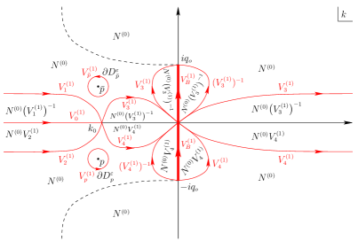
   Figure 4.7. Modulated elliptic wave region in the transmission regime: the first stage of the first deformation. Since $p\in D_{1}$, it is possible to choose the disks $\overline{D_{p}^{\varepsilon}}$ and $\overline{D_{\bar{p}}^{\varepsilon}}$ to always lie in regions where $N^{(1)}=N^{(0)}$.

   The second and the third deformation are identical to the corresponding ones in the plane wave region $\xi<v_{s}$, leading to the function $N^{(3)}(x,t,k)$, which is analytic in $\mathbb{C}\setminus\big{(}\bigcup_{j=1}^{4}L_{j}\cup B\cup\partial D_{p}^{\varepsilon}\cup\partial D_{\bar{p}}^{\varepsilon}\big{)}$ and satisfies the Riemann-Hilbert problem

   $$N^{(3)+} =N^{(3)-}V_{B}^{(3)},\quad k\in B,$$ (4.75eua)

   $$N^{(3)+} =N^{(3)-}V_{j}^{(3)}, k\in L_{j},\ j=1,2,3,4,$$ (4.75eub)

   $$N^{(3)+} =N^{(3)-}V_{p}^{(3)}, k\in\partial D_{p}^{\varepsilon},$$ (4.75euc)

   $$N^{(3)+} =N^{(3)-}V_{\bar{p}}^{(3)}, k\in\partial D_{\bar{p}}^{\varepsilon},$$ (4.75eud)

   $$N^{(3)} =I+O\left(\tfrac{1}{k}\right), k\to\infty,$$ (4.75eue)

   where the contours $L_{j}$ are depicted in Figure 4.8 and the relevant jumps are given by (4.39) and (4.45) but with the function $\delta(\xi,k)$ now modified to

   $$\delta(\xi,k)=\exp\left\{\frac{1}{2i\pi}\int_{-\infty}^{k_{o}(\xi)}\frac{\ln\!\big{[}1+r(\nu)\bar{r}(\nu)\big{]}}{\nu-k}\,d\nu\right\},\quad k\notin(-\infty,k_{o}).$$ (4.75ev)

   Importantly, we note that the jump $V_{3}^{(3)}$ grows exponentially as $t\to\infty$ along the portion of the contour $L_{3}$ colored in green in Figure 4.8, i.e. along the portion of $L_{3}$ that connects $k_{o}$ with the dashed curve $\text{Re}(i\theta)=0$ lying in the second quadrant of the complex $k$-plane. The same is true for the jump $V_{4}^{(3)}$ and the green-colored portion of the contour $L_{4}$ that joins $k_{o}$ with the dashed curve $\text{Re}(i\theta)=0$ in the third quadrant of the complex $k$-plane. This growth, which was not present for $\xi<v_{o}$, can be removed with the help of appropriate factorizations and a time-dependent version of transformation (4.46), as shown in the course of the following two deformations.

   

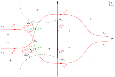
   Figure 4.8. Modulated elliptic wave region in the transmission regime: the jumps of $N^{(3)}$. As $t\to\infty$, the jumps $V_{3}^{(3)}$ and $V_{4}^{(3)}$ grow exponentially along the parts of the contours $L_{3}$ and $L_{4}$ connecting $k_{o}$ with the curve $\text{Re}(i\theta)=0$ (dashed). Moreover, like in the first deformation (see Figure 4.7), the deformed contours do not interfere with the disks $\overline{D_{p}^{\varepsilon}}$ and $\overline{D_{\bar{p}}^{\varepsilon}}$, leaving the corresponding jumps unaffected.

   Fourth deformation. The jumps $V_{3}^{(3)}$ and $V_{4}^{(3)}$ can be factorized in the form

   $$V_{3}^{(3)}=V_{5}^{(4)}V_{7}^{(4)}V_{5}^{(4)},\quad V_{4}^{(3)}=V_{6}^{(4)}V_{8}^{(4)}V_{6}^{(4)},$$ (4.75ew)

   where

   $$V_{5}^{(4)}=\left(\begin{array}[]{lr}1&\frac{\delta^{2}}{r}\,e^{2i\theta t}\\ 0&1\end{array}\right), V_{6}^{(4)}=\left(\begin{array}[]{lr}1&0\\ \frac{1}{\bar{r}\delta^{2}}\,e^{-2i\theta t}&1\end{array}\right),$$ (4.75fb)

   $$V_{7}^{(4)}=\left(\begin{array}[]{lr}0&-\frac{\delta^{2}}{r}\,e^{2i\theta t}\\ \frac{r}{\delta^{2}}\,e^{-2i\theta t}&0\end{array}\right),\quad V_{8}^{(4)}=\left(\begin{array}[]{lr}0&\bar{r}\delta^{2}e^{2i\theta t}\\ -\frac{1}{\bar{r}\delta^{2}}\,e^{-2i\theta t}&0\end{array}\right).$$ (4.75fg)

   The advantage of the above factorization is that the matrices $V_{5}^{(4)}$ and $V_{6}^{(4)}$ each involve only one exponential and hence they have a definitive behavior as $t\to\infty$. In particular, in this limit $V_{5}^{(4)}$ and $V_{6}^{(4)}$ tend to the identity in regions of negative and positive sign of $\text{Re}(i\theta)$ respectively. On the other hand, the matrices $V_{7}^{(4)}$ and $V_{8}^{(4)}$ still involve both of the exponentials $e^{\pm 2i\theta t}$ and so it is not possible to take their limit as $t\to\infty$. However, contrary to the original jumps $V_{3}^{(3)}$ and $V_{4}^{(3)}$, the matrices $V_{7}^{(4)}$ and $V_{8}^{(4)}$ are antidiagonal. This fact turns out to be crucial, as we will see in the fifth deformation below.

   Using the factorization (4.75ew), we switch from $N^{(3)}$ to $N^{(4)}$ as shown in Figure 4.9. By this definition, $N^{(4)}(x,t,k)$ is analytic in $\mathbb{C}\setminus\big{(}\bigcup_{j=1}^{4}L_{j}\cup B\cup\partial D_{p}^{\varepsilon}\cup\partial D_{\bar{p}}^{\varepsilon}\big{)}$ and satisfies the following Riemann-Hilbert problem:

   $$N^{(4)+} =N^{(4)-}V_{B}^{(4)},\quad k\in B,$$ (4.75fha)

   $$N^{(4)+} =N^{(4)-}V_{j}^{(4)}, k\in L_{j},\ j=1,\ldots,8,$$ (4.75fhb)

   $$N^{(4)+} =N^{(4)-}V_{p}^{(4)}, k\in\partial D_{p}^{\varepsilon},$$ (4.75fhc)

   $$N^{(4)+} =N^{(4)-}V_{\bar{p}}^{(4)}, k\in\partial D_{\bar{p}}^{\varepsilon},$$ (4.75fhd)

   $$N^{(4)} =I+O\left(\tfrac{1}{k}\right), k\to\infty,$$ (4.75fhe)

   where the contours $L_{j}$ are shown in Figure 4.9, the jumps $V_{5}^{(4)},V_{6}^{(4)},V_{7}^{(4)},V_{8}^{(4)}$ are given by (4.75fb), and the remaining jumps are as in problem (4.75eu).

   

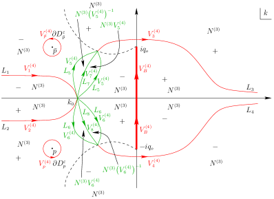
   Figure 4.9. Modulated elliptic wave region in the transmission regime: the fourth deformation. The various jump contours have been chosen so as not to interfere with the disks $\overline{D_{p}^{\varepsilon}}$ and $\overline{D_{\bar{p}}^{\varepsilon}}$.

   The only growth surviving in problem (4.75fh) after the fourth deformation is located in the $21$- and $12$-elements of the jumps $V_{7}^{(4)}$ and $V_{8}^{(4)}$ respectively. The fact that these jumps are antidiagonal allows us to eliminate this growth by employing the following transformation, which is essentially the mechanism leading to a modulated elliptic wave (as opposed to a plane wave).

   Fifth deformation. Let the points $\alpha(\xi)$ and $\bar{\alpha}(\xi)$ be defined through the solution of the modulation equations (2.8), which was shown in [BM2] to be unique for $\xi\in(v_{o},0)$. In turn, let the point $k_{o}(\xi)$ be given by (2.7). Then, introduce the function $h(\xi,k)$ via the Abelian integral (2.5). Note that $h$ involves the function $\gamma(\xi,k)$ defined by (2.9), which is made single-valued by taking branch cuts along $B$ as well as along the curve

   $$\widetilde{B}:=L_{7}\cup(-L_{8})$$ (4.75fi)

   with the contours $L_{7}$ and $L_{8}$ depicted in Figure 4.10. We emphasize that $\widetilde{B}$ must begin at $\bar{\alpha}$ and end at $\alpha$ by crossing the negative real axis at the point $k_{o}$ but is otherwise arbitrary for the moment. The function $\gamma$ is analytic for $k\in\mathbb{C}\setminus B\cup\widetilde{B}$ and changes sign as $k$ crosses $B$ and $\widetilde{B}$. Via (2.5), this induces analyticity of $h$ in $\mathbb{C}\setminus B\cup\widetilde{B}$ as well as the following jump conditions along $B$ and $\widetilde{B}$:

   $$h^{+}+h^{-}=0, k\in B,$$ (4.75fja)

   $$h^{+}+h^{-}=\Omega,\quad k\in L_{7}\cup L_{8},$$ (4.75fjb)

   where the real quantity $\Omega(\xi)$, which is independent of $k$, is defined by

   $$\Omega(\xi)=-4\left(\int_{iq_{o}}^{\alpha}+\int_{-iq_{o}}^{\bar{\alpha}}\right)\frac{\left(z-k_{o}\right)\left(z-\alpha\right)\left(z-\bar{\alpha}\right)}{\gamma(z)}\,dz.$$ (4.75fk)

   Moreover, as shown in [BM2], $\text{Re}(ih)$ has the same sign with $\text{Re}(i\theta)$ at infinity, near the origin, and near $\alpha$ and $\bar{\alpha}$.

   The definition of $h$ and, more specifically, the jump conditions (4.75fj) imply that the jumps of the function

   $$N^{(5)}(x,t,k)=N^{(4)}(x,t,k)e^{-i\left[h(\xi,k)-\theta(\xi,k)\right]t\sigma_{3}}$$ (4.75fl)

   along the contours $L_{7}$ and $L_{8}$ are bounded. Furthermore, those jumps that were bounded at the level of $N^{(4)}$ remain bounded at the level of $N^{(5)}$ (see discussion below (4.75go)). Specifically, Riemann-Hilbert problem (4.75fh) and transformation (4.75fl) imply that $N^{(5)}(x,t,k)$ is analytic for $k\in\mathbb{C}\setminus\big{(}\bigcup_{j=1}^{8}L_{j}\cup B\cup\partial D_{p}^{\varepsilon}\cup\partial D_{\bar{p}}^{\varepsilon}\big{)}$ and satisfies the jump conditions

   $$N^{(5)+} =N^{(5)-}V_{B}^{(5)}, k\in B,$$ (4.75fma)

   $$N^{(5)+} =N^{(5)-}V_{j}^{(5)}, k\in L_{j},\ j=1,\ldots,8,$$ (4.75fmb)

   $$N^{(5)+} =N^{(5)-}V_{p}^{(5)}, k\in\partial D_{p}^{\varepsilon},$$ (4.75fmc)

   $$N^{(5)+} =N^{(5)-}V_{\bar{p}}^{(5)}, k\in\partial D_{\bar{p}}^{\varepsilon},$$ (4.75fmd)

   $$N^{(5)} =\left[I+O\left(\tfrac{1}{k}\right)\right]e^{-iG_{\infty}(\xi)t\sigma_{3}},\quad k\to\infty,$$ (4.75fme)

   where the contours $L_{j}$ are shown in Figure 4.10 and

   $$V_{B}^{(5)}=\left(\begin{array}[]{lr}0&\tfrac{q_{-}}{iq_{o}}\delta^{2}\\ \tfrac{\bar{q}_{-}}{iq_{o}}\delta^{-2}&0\end{array}\right),\quad V_{1}^{(5)}=\left(\begin{array}[]{lr}1&\frac{\bar{r}\delta^{2}}{1+r\bar{r}}\,e^{2iht}\\ 0&1\end{array}\right),\quad V_{2}^{(5)}=\left(\begin{array}[]{lr}1&0\\ \frac{r\delta^{-2}}{1+r\bar{r}}e^{-2iht}&1\end{array}\right),$$ (4.75ft)

   $$V_{3}^{(5)}=\left(\begin{array}[]{lr}1&0\\ r\delta^{-2}e^{-2iht}&1\end{array}\right),\quad V_{4}^{(5)}=\left(\begin{array}[]{lr}1&\bar{r}\delta^{2}e^{2iht}\\ 0&1\end{array}\right),\quad V_{5}^{(5)}=\left(\begin{array}[]{lr}1&\frac{\delta^{2}}{r}\,e^{2iht}\\ 0&1\end{array}\right),$$ (4.75ga)

   $$V_{6}^{(4)}=\left(\begin{array}[]{lr}1&0\\ \frac{1}{\bar{r}\delta^{2}}\,e^{-2iht}&1\end{array}\right),\quad V_{7}^{(5)}=\left(\begin{array}[]{lr}0&-\frac{\delta^{2}}{r}\,e^{i\Omega t}\\ \frac{r}{\delta^{2}}\,e^{-i\Omega t}&0\end{array}\right),\quad V_{8}^{(5)}=\left(\begin{array}[]{lr}0&\bar{r}\delta^{2}e^{i\Omega t}\\ -\frac{1}{\bar{r}\delta^{2}}\,e^{-i\Omega t}&0\end{array}\right),$$ (4.75gh)

   $$V_{p}^{(5)}=\left(\begin{array}[]{lr}1&-\frac{c_{p}\,\delta^{2}(\xi,k)\,d(k)}{k-p}\,e^{2i\left[h(\xi,k)+\theta(\xi,p)-\theta(\xi,k)\right]t}\\ 0&1\end{array}\right),$$ (4.75gk)

   $$V_{\bar{p}}^{(5)}=\left(\begin{array}[]{lr}1&0\\ -\frac{c_{\bar{p}}\,\delta^{-2}(\xi,k)\,d(k)}{k-\bar{p}}\,e^{-2i\left[h(\xi,k)+\theta(\xi,\bar{p})-\theta(\xi,k)\right]t}&1\end{array}\right),$$ (4.75gn)

   with $\Omega(\xi)$ defined by (4.75fk) and the real quantity $G_{\infty}(\xi)$ given by

   $$G_{\infty}(\xi)=-2\left(\int_{iq_{o}}^{\infty}+\int_{-iq_{o}}^{\infty}\right)\left[\frac{\left(z-k_{o}\right)\left(z-\alpha\right)\left(z-\bar{\alpha}\right)}{\gamma(z)}-\left(z-\frac{\xi}{4}\right)\right]dz-q_{o}^{2}.$$ (4.75go)

   

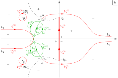
   Figure 4.10. Modulated elliptic wave region in the transmission regime: the fifth deformation.

   Remark 4.1.

   The fourth deformation, which affects only the jumps along the green contours of Figure 4.8 by opening those contours into the lenses comprising the contours $L_{5}$, $L_{6}$, $L_{7}$, $L_{8}$ of Figure 4.9, could also be performed after the $g$-function deformation (4.75fl), leading again to Riemann-Hilbert problem (4.75fm). Nonetheless, the order we have followed here has the advantage of revealing the basic form of the jumps along the contours of growth (see (4.75fb)) before the introduction of the Abelian function $h$, thus allowing us to better motivate the desired properties that eventually lead to the definition of $h$. Of course, since for $v_{o}<\xi<0$ we switch the phase function from $\theta$ to $h$ via deformation (4.75fl), it should be emphasized that the contours $L_{7}$ and $L_{8}$ of Figure 4.10 are not those of Figure 4.9, but rather the contours connecting $\alpha$ and $\bar{\alpha}$ with $k_{o}$.

   The sign structure of $\text{Re}(ih)$ at infinity and near the origin together with the fact that, by definition, $h$ possesses precisely three critical points, namely $k_{o}$, $\alpha$, $\bar{\alpha}$, guarantee the existence of a neighborhood around the point $k_{o}$ where $\text{Re}(ih)<0$ in the second quadrant, $\text{Re}(ih)>0$ in the third quadrant, and $\text{Re}(ih)=0$ along $\mathbb{R}$ and the branch cut $\widetilde{B}$. Thus, thanks to the sign structure of $\text{Re}(ih)$ near $\alpha$, it is always possible to have a contour from $k_{o}$ to $\alpha$ which lies to the right of the branch cut $\widetilde{B}$ and along which $\text{Re}(ih)<0$. Similarly, thanks to the sign structure of $\text{Re}(ih)$ at infinity and near $k_{o}$ and $\alpha$, as well as to the fact that $h$ possesses precisely three critical points, we can always find a contour from $k_{o}$ to $\alpha$ which lies to the left of the branch cut $\widetilde{B}$ and along which $\text{Re}(ih)<0$. Therefore, the contour $L_{5}$ of Figure 4.10 can always be chosen to satisfy $\text{Re}(ih)<0$. In turn, by symmetry, the contour $L_{6}$ can always be chosen to satisfy $\text{Re}(ih)>0$. Hence, the jumps $V_{5}^{(5)}$ and $V_{6}^{(5)}$ are guaranteed to decay exponentially to the identity as $t\to\infty$. Analogous considerations ensure that $\text{Re}(ih)$ has the same sign structure with $\text{Re}(i\theta)$ along the contours $L_{1}$, $L_{2}$, $L_{3}$ and $L_{4}$ of Figure 4.10. Thus, the jumps $V_{1}^{(5)}$, $V_{2}^{(5)}$, $V_{3}^{(5)}$ and $V_{4}^{(5)}$ inherit the behavior of their $N^{(4)}$-counterparts, i.e. they decay exponentially to the identity as $t\to\infty$.

   Furthermore, there exists at least one zero-contour (i.e. a contour along which $\text{Re}(ih)=0$) connecting $\alpha$ and $\bar{\alpha}$ through $k_{o}$. This is because of the sign structure of $\text{Re}(ih)$ near $\alpha$ and $\bar{\alpha}$ as well as due to the jump condition (4.75fjb) along $\widetilde{B}$, which implies that $\text{Re}(ih^{+})=-\text{Re}(ih^{-})$ since $\Omega\in\mathbb{R}$. Thus, either $\widetilde{B}$ is itself a zero-contour, or there exists a region of positive sign adjacent to $\widetilde{B}$ whose boundary will have to be a zero-contour due to the analyticity of $h$, the sign of $\text{Re}(ih)$ at infinity and near the origin, and the existence of precisely three critical points of $h$. In the latter case, we can deform $\widetilde{B}$ to this zero-contour so that $\mathop{\rm Re}(ih)=0$ throughout $\widetilde{B}$. In fact, any zero-contour connecting $\alpha$ and $\bar{\alpha}$ can only cross the negative real axis at $k_{o}$, since a zero-contour intersecting with the negative real axis at a point different than $k_{o}$ would require this point to a critical point, leading to a contradiction. Therefore, taking into account once again the sign structure of $\text{Re}(ih)$ near $\alpha$ and $\bar{\alpha}$, we conclude that for $\xi\in(v_{o},0)$ there exists a unique zero-contour with endpoints $\alpha$ and $\bar{\alpha}$ and through the point $k_{o}$, namely the branch cut $\widetilde{B}$.

   Furthermore, as $\xi$ increases from $v_{o}$ to $0$ the branch cut $\widetilde{B}$ remains within the finite region enclosed by the trace of $\bar{\alpha}$ and $\alpha$ (the dashed green curve in Figure 2.1 and its reflection through the real axis) and the branch cut $B$. Hence, for $p\in D_{1}$, as $\xi$ increases from $v_{o}$ to $0$ the branch cut $\widetilde{B}$ remains to the right of the disks $\overline{D_{p}^{\varepsilon}}$ and $\overline{D_{\bar{p}}^{\varepsilon}}$ without interfering with $p$ and $\bar{p}$. The same is true for $p\in D_{2}^{+}$ since, as shown in Figure 2.1, this region lies by definition below the trace of $\bar{\alpha}$ (while $\widetilde{B}$ lies above that trace). On the other hand, if $p\in D_{2}^{-}\cup D_{3}$ then both $p$ and $\bar{p}$ are crossed by $\widetilde{B}$ for some $\xi\in(v_{o},0)$, this being the mechanism that generates the soliton wake in the mixed regimes of Section 6.

   Next, recall that the transition from $\theta$ to $h$ in the jump matrices takes place at $\xi=v_{o}$, where $h(v_{o},k)=\theta(v_{o},k)$ and $\alpha(v_{o})=\bar{\alpha}(v_{o})=k_{o}(v_{o})=v_{o}/8$. Hence, at $\xi=v_{o}$ the lower and upper dashed curves of Figure 4.10 are, respectively, the solid blue curve of Figure 2.1 and its reflection through the real $k$-axis. A numerical investigation then shows that, as $\xi$ increases from $v_{o}$ to $0$, the upper dashed curve remains convex and moves continuously upwards and to the right, eventually collapsing to the half-line $i[q_{o},\infty)$. Analogously, the lower dashed curve remains concave and moves downwards and to the right, eventually collapsing to the half-line $i(-\infty,-q_{o}]$. Hence, no points inside the regions $D_{1}$ and $D_{3}$ of Figure 2.1 are crossed by the lower dashed curve of Figure 4.10 as $\xi$ increases from $v_{o}$ to $0$. In particular, if $p\in D_{1}\cup D_{3}$, then the circle $\partial D_{p}^{\varepsilon}$, which is between the negative real $k$-axis the solid blue curve of Figure 2.1 at $\xi=v_{o}$, remains below the negative real $k$-axis and above the lower dashed curve of Figure 4.10 throughout the range $(v_{o},0)$. On the other hand, if $p\in D_{2}^{+}\cup D_{2}^{-}$, then it will be crossed at exactly one value of $\xi\in(v_{o},0)$ by the lower dashed curve of Figure 4.10. An analogous statement can be made for $\bar{p}$ by symmetry.

   The dashed curves of Figure 4.10 together with the branch cut $\widetilde{B}$ and the negative real axis make up the contours along which $\text{Re}(ih)=0$ on the left half of the complex $k$-plane. Hence, from the above-described behavior of these contours as $\xi$ increases from $v_{o}$ to $0$, we conclude that

   1. If $p\in D_{1}$, then $\text{Re}(ih)(\xi,p)>0$ for all $\xi\in(v_{o},0)$. Equivalently, the equation

      $$\text{Re}(ih)(\xi,p)=0\Leftrightarrow\text{Re}(ih)(\xi,\bar{p})=0\Leftrightarrow\int_{\bar{p}}^{p}dh(\xi,z)=0$$ (4.75gp)

      has no solution for $\xi\in(v_{o},0)$. Hence, in the transmission regime $p\in D_{1}$ no soliton arises in the range $\xi\in(v_{o},0)$.

   2. If $p\in D_{2}^{+}$, then equation (4.75gp) has a unique solution $\widetilde{v}_{s}\in(v_{o},0)$, which gives rise to a soliton (see Section 5 for more details).

   3. If $p\in D_{2}^{-}$, then equation (4.75gp) has two solutions in the interval $(v_{o},0)$: one due to the crossing of $p$ by the lower dashed curve of 4.10, denoted by $\widetilde{v}_{s}$, and another one due to the crossing of $p$ by the branch cut $\widetilde{B}$, denoted by $v_{w}$. Moreover, $\widetilde{v}_{s}<v_{w}$ and the first solution corresponds to a soliton while the second one to a soliton wake (see Section 6 for more details).

   4. Finally, if $p\in D_{3}$, then equation (4.75gp) has a unique solution $v_{w}\in(v_{o},0)$, which arises from the crossing of $p$ by the branch cut $\widetilde{B}$ and corresponds to a soliton wake (see Section 6 for more details).

   The integral equation (4.75gp) can be expressed in terms of the incomplete elliptic integrals of the first and second kind. Importantly, we note that when the poles coincide with the branch point $\pm iq_{o}$ equation (4.75gp) reduces to the modulation equation (2.8b). A numerical evaluation of the solutions of equation (4.75gp) for various choices of $p$ that cover all four possible regions $D_{1}$, $D_{2}^{+}$, $D_{2}^{-}$ and $D_{3}$ of the third quadrant is shown in Figure 4.11.

   

   

   

   

   

   

   

   

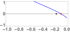
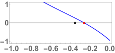
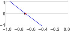
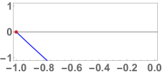
   Figure 4.11. Numerical evaluation of the solutions of equation (4.75gp) for $q_{o}=1$ and the different choices of $p$ depicted by orange dots in Figure 2.1. The horizontal axis corresponds to $\xi$, the vertical axis to $\text{Re}(ih)(\xi,p)$, and the values on both axes are normalized by a factor of $|v_{o}|$ so that the range $[-1,0]$ of $\xi$ corresponds precisely to the modulated elliptic wave region $[v_{o},0]$, where equation (4.75gp) is actually relevant. The black dots denote the unperturbed soliton velocity $v_{s}$ given by (2.10), while the red and blue dots denote the solutions $\widetilde{v}_{s}$ and $v_{w}$ of equation (4.75gp) corresponding to a soliton and a soliton wake respectively. First row: $p=-1.1i\in D_{2}^{+}$ and $p=-0.082-1.1i\in D_{2}^{+}$. Second row: $p=-0.216-1.1i\in D_{2}^{+}$ and $p=-0.69-1.1i\in D_{2}^{+}$. Third row: $p=-1.146-1.1i\in D_{2}^{+}$ and $p=-1.24-1.1i\in D_{1}$. Fourth row: $p=-0.082-0.95i\in D_{2}^{-}$ and $p=-0.214-0.5i\in D_{3}$. Note that in the left panel of the first and third rows $v_{s}$ and $\widetilde{v}_{s}$ essentially coincide. In particular, the latter case, which concerns $D_{2}^{+}$, is in complete agreement with the numerical simulation shown in the center panel of Figure 2.4.

   The only jumps of Riemann-Hilbert problem (4.75fm) that are not bounded as $t\to\infty$ are the ones along $\partial D_{p}^{\varepsilon}$ and $\partial D_{\bar{p}}^{\varepsilon}$, which grow exponentially since they are controlled by the sign of $\text{Re}(ih)(\xi,p)$. Thus, similarly to Subsection 4.3, we must employ the analogue of transformation (4.75db) in order to convert this growth into decay. Before doing so, however, we apply the analogue of transformation (4.46) in order to remove the $k$-dependence from the jumps along $B$ and $\widetilde{B}$. Sixth deformation. The jumps $V_{B}^{(5)}$, $V_{7}^{(5)}$ and $V_{8}^{(5)}$ can be made independent of $k$ by means of the transformation

   $$N^{(6)}(x,t,k)=N^{(5)}(x,t,k)e^{ig(\xi,k)\sigma_{3}},$$ (4.75gq)

   where the function $g(\xi,k)$ is analytic in $\mathbb{C}\setminus(B\cup\widetilde{B})$ and satisfies the following jump conditions:

   $$g^{+}+g^{-} =-i\ln\left(\delta^{2}\right), k\in B,$$ (4.75gra)

   $$g^{+}+g^{-} =-i\ln\left(\tfrac{\delta^{2}}{r}\right)+\omega,\quad k\in L_{7},$$ (4.75grb)

   $$g^{+}+g^{-} =-i\ln\left(\delta^{2}\bar{r}\right)+\omega, k\in L_{8},$$ (4.75grc)

   with $\delta(\xi,k)$ defined by (4.75ev) and with the real quantity $\omega(\xi)$ defined by

   $$\omega(\xi)=i\,\frac{\displaystyle\int_{B}\frac{\ln\delta^{2}(\xi,\nu)}{\gamma(\xi,\nu)}\,d\nu+\int_{\widetilde{B}^{+}}\frac{\ln\left[\frac{\delta^{2}(\xi,\nu)}{r(\nu)}\right]}{\gamma(\xi,\nu)}\,d\nu+\int_{\widetilde{B}^{-}}\frac{\ln\left[\delta^{2}(\xi,\nu)\,\bar{r}(\nu)\right]}{\gamma(\xi,\nu)}\,d\nu}{\displaystyle\int_{\widetilde{B}}\frac{d\nu}{\gamma(\xi,\nu)}},$$ (4.75gs)

   where we have introduced the notation

   $$\widetilde{B}^{\pm}:=\widetilde{B}\cap\mathbb{C}^{\pm}.$$ (4.75gt)

   The solution of problem (4.75gr) is obtained via the Plemelj formulae as

   $$g(\xi,k)=\frac{\gamma(\xi,k)}{2\pi}\bigg{[}\int_{B}\frac{\ln\delta^{2}(\xi,\nu)}{\gamma(\xi,\nu)(\nu-k)}\,d\nu+\int_{L_{7}}\frac{\ln\left[\frac{\delta^{2}(\xi,\nu)}{r(\nu)}\right]+i\omega(\xi)}{\gamma(\xi,\nu)(\nu-k)}\,d\nu-\int_{L_{8}}\frac{\ln\left[\delta^{2}(\xi,\nu)\,\bar{r}(\nu)\right]+i\omega(\xi)}{\gamma(\xi,\nu)(\nu-k)}\,d\nu\bigg{]}.$$ (4.75gu)

   The presence of $\omega$ in the jump conditions (4.75gr) ensures that $g(\xi,k)=O(1)$ as $k\to\infty$. Indeed, expression (4.75gu) implies

   $$g(\xi,k)=g_{\infty}(\xi)+O\left(\frac{1}{k}\right),\quad k\to\infty,$$ (4.75gv)

   where the real quantity $g_{\infty}(\xi)$ is defined by

   $$g_{\infty}(\xi)=-\frac{1}{2\pi}\bigg{[}\int_{B}\frac{\ln\delta^{2}(\xi,\nu)}{\gamma(\xi,\nu)}\,\nu d\nu+\int_{\widetilde{B}^{+}}\frac{\ln\left[\frac{\delta^{2}(\xi,\nu)}{r(\nu)}\right]+i\omega(\xi)}{\gamma(\xi,\nu)}\,\nu d\nu+\int_{\widetilde{B}^{-}}\frac{\ln\left[\delta^{2}(\xi,\nu)\,\bar{r}(\nu)\right]+i\omega(\xi)}{\gamma(\xi,\nu)}\,\nu d\nu\bigg{]}.$$ (4.75gw)

   In summary, the function $N^{(6)}$ defined by (4.75gq) is analytic in $\mathbb{C}\setminus\big{(}\bigcup_{j=1}^{6}L_{j}\cup B\cup\widetilde{B}\cup\partial D_{p}^{\varepsilon}\cup\partial D_{\bar{p}}^{\varepsilon}\big{)}$ and satisfies the Riemann-Hilbert problem

   $$N^{(6)+} =N^{(6)-}V_{B}, k\in B,$$ (4.75gxa)

   $$N^{(6)+} =N^{(6)-}V_{\widetilde{B}}^{(6)}, k\in\widetilde{B},$$ (4.75gxb)

   $$N^{(6)+} =N^{(6)-}V_{j}^{(6)}, k\in L_{j},\ j=1,\ldots,6,$$ (4.75gxc)

   $$N^{(6)+} =N^{(6)-}V_{p}^{(6)}, k\in\partial D_{p}^{\varepsilon},$$ (4.75gxd)

   $$N^{(6)+} =N^{(6)-}V_{\bar{p}}^{(6)}, k\in\partial D_{\bar{p}}^{\varepsilon},$$ (4.75gxe)

   $$N^{(6)} =\left[I+O\left(\tfrac{1}{k}\right)\right]e^{i\left[g_{\infty}(\xi)-G_{\infty}(\xi)t\right]\sigma_{3}},\quad k\to\infty,$$ (4.75gxf)

   where the jump along $B$ is given by (4.8), the jump along $\widetilde{B}$ is equal to

   $$V_{\widetilde{B}}^{(6)}=\left(\begin{array}[]{lr}0&-e^{i(\Omega t-\omega)}\\ e^{-i(\Omega t-\omega)}&0\end{array}\right),$$ (4.75gy)

   the jumps along $\partial D_{p}^{\varepsilon}$ and $\partial D_{\bar{p}}^{\varepsilon}$ are given by

   $$V_{p}^{(6)} =\left(\begin{array}[]{lr}1&-\frac{c_{p}\,\delta^{2}(\xi,k)\,d(k)e^{-2ig(\xi,k)}}{k-p}\,e^{2i\left[h(\xi,k)+\theta(\xi,p)-\theta(\xi,k)\right]t}\\ 0&1\end{array}\right),$$ (4.75gzc)

   $$V_{\bar{p}}^{(6)} =\left(\begin{array}[]{lr}1&0\\ -\frac{c_{\bar{p}}\,\delta^{-2}(\xi,k)\,d(k)e^{2ig(\xi,k)}}{k-\bar{p}}\,e^{-2i\left[h(\xi,k)+\theta(\xi,\bar{p})-\theta(\xi,k)\right]t}&1\end{array}\right),$$ (4.75gzf)

   the jumps along the contours $L_{j}$ of Figure 4.10 are equal to

   $$V_{1}^{(6)} =\left(\begin{array}[]{lr}1&\frac{\bar{r}\,\delta^{2}e^{-2ig}}{1+r\bar{r}}\,e^{2iht}\\ 0&1\end{array}\right),\quad V_{2}^{(6)}=\left(\begin{array}[]{lr}1&0\\ \frac{r\delta^{-2}e^{2ig}}{1+r\bar{r}}\,e^{-2iht}&1\end{array}\right),$$ (4.75hae)

   $$V_{3}^{(6)} =\left(\begin{array}[]{lr}1&0\\ r\delta^{-2}e^{2ig}e^{-2iht}&1\end{array}\right),\quad V_{4}^{(6)}=\left(\begin{array}[]{lr}1&\bar{r}\delta^{2}e^{-2ig}e^{2iht}\\ 0&1\end{array}\right),$$ (4.75haj)

   $$V_{5}^{(6)} =\left(\begin{array}[]{lr}1&\frac{\delta^{2}e^{-2ig}}{r}\,e^{2iht}\\ 0&1\end{array}\right),\quad V_{6}^{(6)}=\left(\begin{array}[]{lr}1&0\\ \frac{\delta^{-2}e^{2ig}}{\bar{r}}\,e^{-2iht}&1\end{array}\right),$$ (4.75hao)

   and the real quantities $G_{\infty}(\xi)$ and $g_{\infty}(\xi)$ are given by (4.75go) and (4.75gw) respectively. Converting growth into decay. The growing exponentials in the jumps $V_{p}^{(6)}$ and $V_{\bar{p}}^{(6)}$ can be converted into decaying ones via the analogue of transformation (4.75db), i.e. by letting

   $$\widetilde{N}^{(6)}=\begin{cases}N^{(6)}n^{\sigma_{3}},&k\in\mathbb{C}\setminus\left(\,\overline{D_{p}^{\varepsilon}}\cup\overline{D_{\bar{p}}^{\varepsilon}}\,\right),\\ N^{(6)}J_{p}\,n^{\sigma_{3}},&k\in D_{p}^{\varepsilon},\\ N^{(6)}J_{\bar{p}}\,n^{\sigma_{3}},&k\in D_{\bar{p}}^{\varepsilon},\end{cases}$$ (4.75hba)

   where

   $$J_{p}(\xi,k) =\left(\begin{array}[]{lr}\dfrac{1-\frac{n^{2}(p)}{n^{2}(k)}}{k-p}&c_{p}\,d(k)\delta^{2}(\xi,k)e^{2i\left[\left(h(\xi,k)+\theta(\xi,p)-\theta(\xi,k)\right)t-g\right]}\\ -\dfrac{n^{2}(p)\,e^{-2i\left[\left(h(\xi,k)+\theta(\xi,p)-\theta(\xi,k)\right)t-g\right]}}{c_{p}\,d(k)\delta^{2}(\xi,k)\left(k-\bar{p}\right)^{2}}&k-p\end{array}\right),$$ (4.75hbd)

   $$J_{\bar{p}}(\xi,k) =\left(\begin{array}[]{lr}k-\bar{p}&-\dfrac{e^{2i\left[\left(h(\xi,k)+\theta(\xi,\bar{p})-\theta(\xi,k)\right)t-g\right]}}{n^{2}(\bar{p})c_{\bar{p}}\,d(k)\delta^{-2}(\xi,k)\left(k-p\right)^{2}}\\ c_{\bar{p}}\,d(k)\delta^{-2}(\xi,k)e^{-2i\left[\left(h(\xi,k)+\theta(\xi,\bar{p})-\theta(\xi,k)\right)t-g\right]}&\dfrac{1-\frac{n^{2}(k)}{n^{2}(\bar{p})}}{k-\bar{p}}\end{array}\right).$$ (4.75hbg)

   Then, $\widetilde{N}^{(6)}$ satisfies the Riemann-Hilbert problem

   $$\widetilde{N}^{(6)+} =\widetilde{N}^{(6)-}\widetilde{V}_{B}^{(6)}, k\in B,$$ (4.75hca)

   $$\widetilde{N}^{(6)+} =\widetilde{N}^{(6)-}\widetilde{V}_{\widetilde{B}}^{(6)}, k\in\widetilde{B},$$ (4.75hcb)

   $$\widetilde{N}^{(6)+} =\widetilde{N}^{(6)-}\widetilde{V}_{j}^{(6)}, k\in L_{j},\ j=1,\ldots,6,$$ (4.75hcc)

   $$\widetilde{N}^{(6)+} =\widetilde{N}^{(6)-}\widetilde{V}_{p}^{(6)}, k\in\partial D_{p}^{\varepsilon},$$ (4.75hcd)

   $$\widetilde{N}^{(6)+} =\widetilde{N}^{(6)-}\widetilde{V}_{\bar{p}}^{(6)}, k\in\partial D_{\bar{p}}^{\varepsilon},$$ (4.75hce)

   $$\widetilde{N}^{(6)} =\left[I+O\left(\tfrac{1}{k}\right)\right]e^{i\left[g_{\infty}(\xi)-G_{\infty}(\xi)t\right]\sigma_{3}},\quad k\to\infty,$$ (4.75hcf)

   where the jumps along $B$ and $\widetilde{B}$ are given by

   $$\widetilde{V}_{B}^{(6)}=\left(\begin{array}[]{lr}0&\tfrac{q_{-}}{iq_{o}}n^{-2}\\ \tfrac{\bar{q}_{-}}{iq_{o}}n^{2}&0\end{array}\right),\quad\widetilde{V}_{\widetilde{B}}^{(6)}=\left(\begin{array}[]{lr}0&-e^{i(\Omega t-\omega)}n^{-2}\\ e^{-i(\Omega t-\omega)}n^{2}&0\end{array}\right),$$ (4.75hd)

   the jumps along $\partial D_{p}^{\varepsilon}$ and $\partial D_{\bar{p}}^{\varepsilon}$ are equal to

   $$\widetilde{V}_{p}^{(6)} =\left(\begin{array}[]{lr}1&0\\ -\dfrac{n^{2}(p)e^{2ig(\xi,k)}}{c_{p}\,\delta^{2}(\xi,k)\,d(k)(k-p)}\,e^{-2i\left[h(\xi,k)+\theta(\xi,p)-\theta(\xi,k)\right]t}&1\end{array}\right),$$ (4.75hec)

   $$\widetilde{V}_{\bar{p}}^{(6)} =\left(\begin{array}[]{lr}1&-\dfrac{n^{-2}(\bar{p})\,\delta^{2}(\xi,k)e^{-2ig(\xi,k)}}{c_{\bar{p}}\,d(k)(k-\bar{p})}\,e^{2i\left[h(\xi,k)+\theta(\xi,\bar{p})-\theta(\xi,k)\right]t}\\ 0&1\end{array}\right),$$ (4.75hef)

   and the jumps along the contours $L_{j}$ of Figure 4.10 are given by

   $$\widetilde{V}_{1}^{(6)} =\left(\begin{array}[]{lr}1&\dfrac{\bar{r}\,\delta^{2}e^{-2ig}}{1+r\bar{r}}\,e^{2iht}n^{-2}\\ 0&1\end{array}\right),\quad \widetilde{V}_{2}^{(6)}=\left(\begin{array}[]{lr}1&0\\ \frac{r\delta^{-2}e^{2ig}}{1+r\bar{r}}\,e^{-2iht}n^{2}&1\end{array}\right),$$ (4.75hfe)

   $$\widetilde{V}_{3}^{(6)} =\left(\begin{array}[]{lr}1&0\\ r\delta^{-2}e^{2ig}e^{-2iht}n^{2}&1\end{array}\right),\quad \widetilde{V}_{4}^{(6)}=\left(\begin{array}[]{lr}1&\bar{r}\delta^{2}e^{-2ig}e^{2iht}n^{-2}\\ 0&1\end{array}\right),$$ (4.75hfj)

   $$\widetilde{V}_{5}^{(6)} =\left(\begin{array}[]{lr}1&\frac{\delta^{2}e^{-2ig}}{r}\,e^{2iht}n^{-2}\\ 0&1\end{array}\right),\quad \widetilde{V}_{6}^{(6)}=\left(\begin{array}[]{lr}1&0\\ \frac{\delta^{-2}e^{2ig}}{\bar{r}}\,e^{-2iht}n^{2}&1\end{array}\right).$$ (4.75hfo)

   Transformation (4.75hb) has re-introduced $k$ in the jumps along $B$ and $\widetilde{B}$, which had been made $k$-independent via the sixth deformation. Thus, motivated by the plane wave region, where having a constant jump along $B$ allowed us to solve the dominant Riemann-Hilbert problem explicitly, we next perform a final, seventh deformation in order to remove the $k$-dependence from the jumps $\widetilde{V}_{B}^{(6)}$ and $\widetilde{V}_{\widetilde{B}}^{(6)}$.

   Remark 4.2 (Order of deformations).

   In view of the above discussion, it becomes apparent that the sixth deformation should have been postponed until after transformation (4.75hb), since then the $k$-dependence from the jumps along $B$ and $\widetilde{B}$ would have to be removed only once instead of twice. However, the less efficient order of deformations that we have followed has the advantage of revealing precisely which part of the overall phase of the modulated elliptic wave (2.19) is generated by the soliton at $\xi=v_{s}$ (namely, the constant $4\textnormal{arg}\left[p+\lambda(p)\right]$ via the seventh deformation as shown in (4.75hm)).

   Seventh deformation. Similarly to (4.75gq), we eliminate the dependence on $k$ from the jumps $\widetilde{V}_{B}^{(6)}$ and $\widetilde{V}_{\widetilde{B}}^{(6)}$ by letting

   $$\widetilde{N}^{(7)}(x,t,k)=\widetilde{N}^{(6)}(x,t,k)e^{i\widetilde{g}(\xi,k)\sigma_{3}},$$ (4.75hg)

   where the function $\widetilde{g}(\xi,k)$ is analytic in $\mathbb{C}\setminus(B\cup\widetilde{B})$ and satisfies the jump conditions

   $$\widetilde{g}^{\,+}+\widetilde{g}^{\,-} =i\ln\left(n^{2}\right), k\in B,$$ (4.75hha)

   $$\widetilde{g}^{\,+}+\widetilde{g}^{\,-} =i\ln\left(n^{2}r\right)+\widetilde{\omega},\quad k\in L_{7},$$ (4.75hhb)

   $$\widetilde{g}^{\,+}+\widetilde{g}^{\,-} =i\ln\left(\tfrac{n^{2}}{\bar{r}}\right)+\widetilde{\omega}, k\in L_{8},$$ (4.75hhc)

   with the real quantity $\widetilde{\omega}(\xi)$ given by

   $$\widetilde{\omega}(\xi)=-i\,\frac{\displaystyle\int_{B}\frac{\ln n^{2}(\nu)}{\gamma(\xi,\nu)}\,d\nu+\int_{L_{7}}\frac{\ln\left[n^{2}(\nu)r(\nu)\right]}{\gamma(\xi,\nu)}\,d\nu+\int_{L_{8}}\frac{\ln\left[\frac{\bar{r}(\nu)}{n^{2}(\nu)}\right]}{\gamma(\xi,\nu)}\,d\nu}{\displaystyle\int_{\widetilde{B}}\frac{d\nu}{\gamma(\xi,\nu)}}.$$ (4.75hi)

   Similarly to (4.75gu), we have the explicit formula

   $$\widetilde{g}(\xi,k)=-\frac{\gamma(\xi,k)}{2\pi}\bigg{\{}\int_{B}\frac{\ln n^{2}(\nu)}{\gamma(\xi,\nu)(\nu-k)}\,d\nu+\int_{L_{7}}\frac{\ln\left[n^{2}(\nu)r(\nu)\right]-i\widetilde{\omega}(\xi)}{\gamma(\xi,\nu)(\nu-k)}\,d\nu+\int_{L_{8}}\frac{\ln\left[\frac{\bar{r}(\nu)}{n^{2}(\nu)}\right]+i\widetilde{\omega}(\xi)}{\gamma(\xi,\nu)(\nu-k)}\,d\nu\bigg{\}},$$ (4.75hj)

   which implies

   $$\widetilde{g}(\xi,k)=\widetilde{g}_{\infty}(\xi)+O\left(\frac{1}{k}\right),\quad k\to\infty,$$ (4.75hk)

   with the real quantity $\widetilde{g}_{\infty}(\xi)$ given by

   $$\widetilde{g}_{\infty}(\xi)=\frac{1}{2\pi}\bigg{\{}\int_{B}\frac{\ln n^{2}(\nu)}{\gamma(\xi,\nu)}\,\nu d\nu+\int_{L_{7}}\frac{\ln\left[n^{2}(\nu)r(\nu)\right]-i\widetilde{\omega}(\xi)}{\gamma(\xi,\nu)}\,\nu d\nu+\int_{L_{8}}\frac{\ln\left[\frac{\bar{r}(\nu)}{n^{2}(\nu)}\right]+i\widetilde{\omega}(\xi)}{\gamma(\xi,\nu)}\,\nu d\nu\bigg{\}}.$$ (4.75hl)

   It turns out that $\widetilde{g}_{\infty}$ is actually independent of $\xi$ and, more precisely,

   $$\widetilde{g}_{\infty}=2\text{arg}\left[p+\lambda(p)\right]$$ (4.75hm)

   like in the plane wave region. Eventually (see Remark 4.5), this implies that the effect of the soliton at $\xi=v_{o}$ on the phase of the leading order asymptotics is the same both for $\xi\in(v_{o},0)$ and for $\xi\in(v_{s},v_{o})$.

   The Riemann-Hilbert problem for $\widetilde{N}^{(6)}$ yields the following problem for $\widetilde{N}^{(7)}$:

   $$\widetilde{N}^{(7)+} =\widetilde{N}^{(7)-}V_{B}, k\in B,$$ (4.75hna)

   $$\widetilde{N}^{(7)+} =\widetilde{N}^{(7)-}\widetilde{V}_{\widetilde{B}}^{(7)}, k\in\widetilde{B},$$ (4.75hnb)

   $$\widetilde{N}^{(7)+} =\widetilde{N}^{(7)-}\widetilde{V}_{j}^{(7)}, k\in L_{j},\ j=1,\ldots,6,$$ (4.75hnc)

   $$\widetilde{N}^{(7)+} =\widetilde{N}^{(7)-}\widetilde{V}_{p}^{(7)}, k\in\partial D_{p}^{\varepsilon},$$ (4.75hnd)

   $$\widetilde{N}^{(7)+} =\widetilde{N}^{(7)-}\widetilde{V}_{\bar{p}}^{(7)}, k\in\partial D_{\bar{p}}^{\varepsilon},$$ (4.75hne)

   $$\widetilde{N}^{(7)} =\left[I+O\left(\tfrac{1}{k}\right)\right]e^{i\left[g_{\infty}(\xi)+\widetilde{g}_{\infty}-G_{\infty}(\xi)t\right]\sigma_{3}},\quad k\to\infty,$$ (4.75hnf)

   where the jump along $B$ is given by (4.8), the jump along $\widetilde{B}$ is equal to

   $$\widetilde{V}_{\widetilde{B}}^{(7)}=\left(\begin{array}[]{lr}0&-e^{i(\Omega t-\omega-\widetilde{\omega})}\\ e^{-i(\Omega t-\omega-\widetilde{\omega})}&0\end{array}\right)$$ (4.75ho)

   with the real quantities $\Omega$, $\omega$ and $\widetilde{\omega}$ given by (4.75fk), (4.75gs) and (4.75hi) respectively, the jumps along $\partial D_{p}^{\varepsilon}$ and $\partial D_{\bar{p}}^{\varepsilon}$ are given by

   $$\widetilde{V}_{p}^{(7)} =\left(\begin{array}[]{lr}1&0\\ -\dfrac{n^{2}(p)e^{2i\left[g(\xi,k)+\widetilde{g}(\xi,k)\right]}}{c_{p}\,\delta^{2}(\xi,k)\,d(k)(k-p)}\,e^{-2i\left[h(\xi,k)+\theta(\xi,p)-\theta(\xi,k)\right]t}&1\end{array}\right),$$ (4.75hpc)

   $$\widetilde{V}_{\bar{p}}^{(7)} =\left(\begin{array}[]{lr}1&-\dfrac{n^{-2}(\bar{p})\,\delta^{2}(\xi,k)e^{-2i\left[g(\xi,k)+\widetilde{g}(\xi,k)\right]}}{c_{\bar{p}}\,d(k)(k-\bar{p})}\,e^{2i\left[h(\xi,k)+\theta(\xi,\bar{p})-\theta(\xi,k)\right]t}\\ 0&1\end{array}\right)$$ (4.75hpf)

   with the functions $d$, $n$, $\delta$, $g$ and $\widetilde{g}$ defined by (3.4), (4.75db), (4.75ev), (4.75gu) and (4.75hj) respectively, the jumps along the contours $L_{j}$ of Figure 4.10 are given by

   $$\widetilde{V}_{1}^{(7)} =\left(\begin{array}[]{lr}1&\frac{\bar{r}\,\delta^{2}e^{-2i(g+\widetilde{g})}}{1+r\bar{r}}\,e^{2iht}n^{-2}\\ 0&1\end{array}\right),\quad \widetilde{V}_{2}^{(7)}=\left(\begin{array}[]{lr}1&0\\ \frac{r\delta^{-2}e^{2i(g+\widetilde{g})}}{1+r\bar{r}}\,e^{-2iht}n^{2}&1\end{array}\right),$$ (4.75hqe)

   $$\widetilde{V}_{3}^{(7)} =\left(\begin{array}[]{lr}1&0\\ r\delta^{-2}e^{2i(g+\widetilde{g})}e^{-2iht}n^{2}&1\end{array}\right),\quad \widetilde{V}_{4}^{(7)}=\left(\begin{array}[]{lr}1&\bar{r}\delta^{2}e^{-2i(g+\widetilde{g})}e^{2iht}n^{-2}\\ 0&1\end{array}\right),$$ (4.75hqj)

   $$\widetilde{V}_{5}^{(7)} =\left(\begin{array}[]{lr}1&\frac{\delta^{2}e^{-2i(g+\widetilde{g})}}{r}\,e^{2iht}n^{-2}\\ 0&1\end{array}\right),\quad \widetilde{V}_{6}^{(7)}=\left(\begin{array}[]{lr}1&0\\ \frac{\delta^{-2}e^{2i(g+\widetilde{g})}}{\bar{r}}\,e^{-2iht}n^{2}&1\end{array}\right),$$ (4.75hqo)

   the real quantities $G_{\infty}$ and $g_{\infty}$ are defined by (4.75go) and (4.75gw), and the real constant $\widetilde{g}_{\infty}$ is given by (4.75hm).

   Decomposition into dominant and error problems. The jumps $\widetilde{V}_{j}^{(7)}$, $j=1,\ldots,6$, do not contribute to the leading-order long-time asymptotics since they decay to the identity as $t\to\infty$ due to the sign structure of $\mathop{\rm Re}(ih)$ (see Figure 4.10). The same is true for the jumps $\widetilde{V}_{p}^{(7)}$ and $\widetilde{V}_{\bar{p}}^{(7)}$ since the exponentials involved in these jumps are controlled by the sign of $\text{Re}(ih)(\xi,p)$.${}^{\ref{ds-p-foot}}$ Therefore, the dominant component of Riemann-Hilbert problem (4.75hn) must come from the jumps $V_{B}$ and $\widetilde{V}_{\widetilde{B}}^{(7)}$. With these in mind, we decompose problem (4.75hn) as follows.

   Let $D_{k_{o}}^{\epsilon}$, $D_{\alpha}^{\epsilon}$ and $D_{\bar{\alpha}}^{\epsilon}$ be disks of radius $\epsilon$ centered at $k_{o}$, $\alpha$ and $\bar{\alpha}$ respectively, where $\epsilon$ is sufficiently small so that these disks do not intersect with each other or with $B\cup\overline{D_{p}^{\varepsilon}}\cup\overline{D_{p}^{\varepsilon}}$. Then, write

   $$\widetilde{N}^{(7)}=\widetilde{N}^{\textnormal{err}}\widetilde{N}^{\textnormal{asymp}}$$ (4.75hr)

   where

   $$\widetilde{N}^{\textnormal{asymp}}=\begin{cases}\widetilde{N}^{\textnormal{dom}},&k\in\mathbb{C}\setminus(D_{k_{o}}^{\epsilon}\cup D_{\alpha}^{\epsilon}\cup D_{\bar{\alpha}}^{\epsilon}),\\ \widetilde{N}^{D},&k\in D_{k_{o}}^{\epsilon}\cup D_{\alpha}^{\epsilon}\cup D_{\bar{\alpha}}^{\epsilon},\end{cases}$$ (4.75hs)

   and the functions $\widetilde{N}^{\textnormal{dom}}$, $\widetilde{N}^{D}$ and $\widetilde{N}^{\textnormal{err}}$ are defined as follows:

   1. $\widetilde{N}^{\textnormal{dom}}(x,t,k)$ is analytic in $\mathbb{C}\setminus(B\cup\widetilde{B})$ and satisfies the Riemann-Hilbert problem

      $$\widetilde{N}^{{\textnormal{dom}}+} =\widetilde{N}^{{\textnormal{dom}}-}V_{B}, k\in B,$$ (4.75hta)

      $$\widetilde{N}^{{\textnormal{dom}}+} =\widetilde{N}^{{\textnormal{dom}}-}\widetilde{V}_{\widetilde{B}}^{(7)}, k\in\widetilde{B},$$ (4.75htb)

      $$\widetilde{N}^{\textnormal{dom}} =\left[I+O\left(\tfrac{1}{k}\right)\right]e^{i\left[g_{\infty}(\xi)+\widetilde{g}_{\infty}-G_{\infty}(\xi)t\right]\sigma_{3}},\quad k\to\infty.$$ (4.75htc)

   2. $\widetilde{N}^{D}(x,t,k)$ is analytic in $D_{k_{o}}^{\epsilon}\cup D_{\alpha}^{\epsilon}\cup D_{\bar{\alpha}}^{\epsilon}\setminus\bigcup_{j=1}^{8}L_{j}$ with jumps

      $$\widetilde{N}^{D+}=\widetilde{N}^{D-}\widetilde{V}_{j}^{(6)},\quad k\in\widehat{L}_{j}:=L_{j}\cap\left(D_{k_{o}}^{\epsilon}\cup D_{\alpha}^{\epsilon}\cup D_{\bar{\alpha}}^{\epsilon}\right),\ j=1,\ldots,8,$$ (4.75hu)

      as shown in Figure 4.12.

      

      

      

      Figure 4.12. Modulated elliptic wave in the transmission regime: The jumps of $\widetilde{N}^{D}$ in the interior of and along the boundary of the disks $\overline{D_{\alpha}^{\epsilon}}$, $\overline{D_{\bar{\alpha}}^{\epsilon}}$ and $\overline{D_{k_{o}}^{\epsilon}}$. Note that, although the jumps $\widetilde{V}_{D_{\alpha}}^{\textnormal{asymp}}$, $\widetilde{V}_{D_{\bar{\alpha}}}^{\textnormal{asymp}}$, $\widetilde{V}_{D_{k_{o}}}^{\textnormal{asymp}}$ are unknown, they are equal to the identity up to $O(t^{-1/2})$ and hence do not affect the dominant problem.

   3. $\widetilde{N}^{\textnormal{err}}(x,t,k)$ is analytic in $\mathbb{C}\setminus(\bigcup_{j=1}^{6}\savestack{\tmpbox}{\stretchto{\scaleto{\scalerel*[width("L")]{\kern-0.6pt\bigwedge\kern-0.6pt}{\rule[-505.89pt]{4.30554pt}{505.89pt}}}{}}{0.5ex}}\stackon[1pt]{L}{\scalebox{-1.0}{\tmpbox}}_{j}\cup\partial D_{k_{o}}^{\epsilon}\cup\partial D_{\alpha}^{\epsilon}\cup\partial D_{\bar{\alpha}}^{\epsilon}\cup\partial D_{p}^{\varepsilon}\cup\partial D_{\bar{p}}^{\varepsilon}\big{)}$ with $\savestack{\tmpbox}{\stretchto{\scaleto{\scalerel*[width("L")]{\kern-0.6pt\bigwedge\kern-0.6pt}{\rule[-505.89pt]{4.30554pt}{505.89pt}}}{}}{0.5ex}}\stackon[1pt]{L}{\scalebox{-1.0}{\tmpbox}}_{j}:=L_{j}\setminus(\overline{D_{k_{o}}^{\epsilon}}\cup\overline{D_{\alpha}^{\epsilon}}\cup\overline{D_{\bar{\alpha}}^{\epsilon}})$ and satisfies the Riemann-Hilbert problem (see Figure 4.13)

      $$\widetilde{N}^{{\textnormal{err}}+} =\widetilde{N}^{{\textnormal{err}}-}\widetilde{V}^{\textnormal{err}},\quad$$

      $$\widetilde{N}^{\textnormal{err}} =I+O\left(\tfrac{1}{k}\right), k\to\infty,$$ (4.75hva)

      where

      $$\widetilde{V}^{\textnormal{err}}=\begin{cases}\widetilde{N}^{\textnormal{dom}}\widetilde{V}_{j}^{(7)}(\widetilde{N}^{\textnormal{dom}})^{-1},&k\in\savestack{\tmpbox}{\stretchto{\scaleto{\scalerel*[width("L")]{\kern-0.6pt\bigwedge\kern-0.6pt}{\rule[-505.89pt]{4.30554pt}{505.89pt}}}{}}{0.5ex}}\stackon[1pt]{L}{\scalebox{-1.0}{\tmpbox}}_{j},\\ \widetilde{N}^{\textnormal{dom}}\widetilde{V}_{p}^{(7)}(\widetilde{N}^{\textnormal{dom}})^{-1},&k\in\partial D_{p}^{\varepsilon},\\ \widetilde{N}^{\textnormal{dom}}\widetilde{V}_{\bar{p}}^{(7)}(\widetilde{N}^{\textnormal{dom}})^{-1},&k\in\partial D_{\bar{p}}^{\varepsilon},\\ \widetilde{N}^{{\textnormal{asymp}}-}(\widetilde{V}_{D}^{\textnormal{asymp}})^{-1}(\widetilde{N}^{{\textnormal{asymp}}-})^{-1},&k\in\partial D_{k_{o}}^{\epsilon}\cup\partial D_{\alpha}^{\epsilon}\cup\partial D_{\bar{\alpha}}^{\epsilon},\end{cases}$$ (4.75hvhw)

      and

      $$\widetilde{V}_{D}^{\textnormal{asymp}}=\begin{cases}\widetilde{V}_{D_{\alpha}}^{\textnormal{asymp}},&k\in\partial D_{\alpha}^{\epsilon},\\ \widetilde{V}_{D_{\bar{\alpha}}}^{\textnormal{asymp}},&k\in\partial D_{\bar{\alpha}}^{\epsilon},\\ \widetilde{V}_{D_{k_{o}}}^{\textnormal{asymp}},&k\in\partial D_{k_{o}}^{\epsilon}.\end{cases}$$ (4.75hvhx)

      Importantly, despite the fact that the jump $\widetilde{V}_{D}^{\textnormal{asymp}}$ is unknown, in [BM2] it was estimated to be equal to the identity up to $O(t^{-1/2})$ and hence it does not affect the leading-order asymptotics.

      

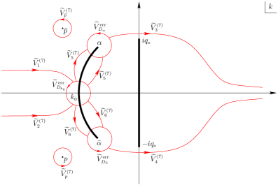
      Figure 4.13. Modulated elliptic wave in the transmission regime: The jumps of $\widetilde{N}^{\textnormal{err}}$.

      Solution of the dominant problem. We begin by noting that, at the level of the dominant problem (4.75ht), since the jump $\widetilde{V}_{\widetilde{B}}^{(7)}$ is independent of $k$, the jump contour $\widetilde{B}$ can be deformed to the straight line segment $B^{\prime}$ from $\bar{\alpha}$ to $\alpha$ so that the jump contours of problem (4.75ht) are as shown in Figure 4.14.

      

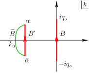
      Figure 4.14. Modulated elliptic wave in the transmission regime: The jump contours of $\widetilde{N}^{\textnormal{dom}}$. The fact that the jump $\widetilde{V}_{\widetilde{B}}^{(7)}$ is independent of $k$ has allowed us to deform $\widetilde{B}$ to the straight line segment $B^{\prime}$ from $\bar{\alpha}$ to $\alpha$. Note that the original and deformed versions of $\widetilde{N}^{\textnormal{dom}}$ agree outside the finite region $\mathcal{D}$ enclosed by $\widetilde{B}$ and $B^{\prime}$.

      Problem (4.75ht) was solved in [BM2] in the case of $\widetilde{\omega}=\widetilde{g}_{\infty}=0$. Adapting that analysis to account for the presence of $\widetilde{\omega}$ and $\widetilde{g}_{\infty}$, we obtain

      $$\widetilde{N}^{\textnormal{dom}}(x,t,k)=e^{i\left[g_{\infty}(\xi)+\widetilde{g}_{\infty}-G_{\infty}(\xi)t\right]\sigma_{3}}\widetilde{\mathcal{N}}^{-1}(\xi,\infty,c)\,\widetilde{\mathcal{N}}(\xi,k,c)$$ (4.75hvhy)

      with

      $$\widetilde{\mathcal{N}}(\xi,k,c)=\frac{1}{2}\left(\begin{array}[]{lr}\left[\eta(\xi,k)+\eta^{-1}(\xi,k)\right]{\mathbf{\widetilde{N}}}_{1}(\xi,k,c)&i\left[\eta(\xi,k)-\eta^{-1}(\xi,k)\right]{\mathbf{\widetilde{N}}}_{2}(\xi,k,c)\\ -i\left[\eta(\xi,k)-\eta^{-1}(\xi,k)\right]{\mathbf{\widetilde{N}}}_{1}(\xi,k,-c)&\left[\eta(\xi,k)+\eta^{-1}(\xi,k)\right]{\mathbf{\widetilde{N}}}_{2}(\xi,k,-c)\end{array}\right)$$ (4.75hvhz)

      and

      $$\widetilde{\mathcal{N}}(\xi,\infty,c):=\lim_{k\to\infty}\widetilde{\mathcal{N}}(\xi,k,c),$$ (4.75hvia)

      where the function $\eta$ with branch cuts along $B$ and $B^{\prime}$ (see Figure 4.14) is defined by

      $$\eta(\xi,k):=\left[\frac{\left(k-iq_{o}\right)\left(k-\alpha\right)}{\left(k+iq_{o}\right)\left(k-\bar{\alpha}\right)}\right]^{\frac{1}{4}}$$ (4.75hvib)

      and where ${\mathbf{\widetilde{N}}}_{1}$ and ${\mathbf{\widetilde{N}}}_{2}$ denote the first and second component of the vector-valued function

      $${\mathbf{\widetilde{N}}}(\xi,k,c):=\left(\frac{\Theta\big{(}-\frac{\Omega t}{2\pi}+\frac{\omega+\widetilde{\omega}}{2\pi}+\frac{i\ln\left(\frac{\bar{q}_{-}}{iq_{o}}\right)}{2\pi}+\upnu(k)+c\big{)}}{\sqrt{\frac{iq_{o}}{\bar{q}_{-}}}\ \Theta\left(\upnu(k)+c\right)},\frac{\Theta\big{(}-\frac{\Omega t}{2\pi}+\frac{\omega+\widetilde{\omega}}{2\pi}+\frac{i\ln\left(\frac{\bar{q}_{-}}{iq_{o}}\right)}{2\pi}-\upnu(k)+c\big{)}}{\sqrt{\tfrac{\bar{q}_{-}}{iq_{o}}}\ \Theta\left(-\upnu(k)+c\right)}\right).$$ (4.75hvic)

      In the above definition, the dependence of $\Omega$, $\omega$, $\widetilde{\omega}$, $\upnu$ and $c$ on $\xi$ has been suppressed for convenience. Moreover, $\Theta(k)=\Theta(\xi,k)$ is the following variant of the third Jacobi theta function:

      $$\Theta(\xi,k)=\theta_{3}(\pi k,e^{i\pi\tau(\xi)}),\quad\theta_{3}(z,\varrho):=\sum_{\ell\in\mathbb{Z}}e^{2i\ell z}\varrho^{\ell^{2}},$$ (4.75hvid)

      with Riemann period

      $$\tau(\xi):=\left(\oint_{\upbeta}\frac{dk}{\Gamma(\xi,k)}\right)^{-1}\oint_{\upalpha}\frac{dk}{\Gamma(\xi,k)}=\frac{iK\big{(}\sqrt{1-m^{2}}\,\big{)}}{K\left(m\right)},$$ (4.75hvie)

      where the function $\Gamma$ is defined in terms of the function $\gamma$ of (2.9) by

      $$\Gamma(\xi,k)=\left\{\begin{array}[]{ll}\gamma(\xi,k),&k\in\mathbb{C}\setminus\overline{\mathcal{D}},\\ -\gamma(\xi,k),&k\in\mathcal{D},\end{array}\right.$$ (4.75hvif)

      where $\mathcal{D}$ denotes the finite region enclosed by $\widetilde{B}$ and $B^{\prime}$ (see Figure 4.14). This definition implies that $\Gamma$ has branch cuts along $B$ and $B^{\prime}$, i.e. the branch cut $\widetilde{B}$ of $\gamma$ has been deformed to $B^{\prime}$ in the case of $\Gamma$. The cycles $\{\upalpha,\upbeta\}$ of the genus-1 Riemann surface associated with $\Gamma$ are depicted in Figure 4.15. Furthermore, the Abelian map $\upnu$ in the arguments of the $\Theta$-functions in (4.75hvic) is defined by

      $$\upnu(k)=\upnu(\xi,k)=\left(\oint_{\upbeta}\frac{d\nu}{\Gamma(\xi,\nu)}\right)^{-1}\int_{iq_{o}}^{k}\frac{d\nu}{\Gamma(\xi,\nu)},$$ (4.75hvig)

      and, finally,

      $$c=c(\xi):=\upnu\!\left(\frac{q_{o}\alpha_{\textnormal{re}}}{q_{o}+\alpha_{\textnormal{im}}}\right)+\frac{1}{2}\left(1+\tau\right).$$ (4.75hvih)

      Remark 4.3 (Analyticity of $\widetilde{\mathcal{N}}(\xi,k,c)$).

      The definition (4.75hvih) of $c$ ensures that the only possible singularity of $\widetilde{\mathcal{N}}(\xi,k,c)$ on the first sheet of the Riemann surface may occur at $k=\frac{q_{o}\alpha_{\textnormal{re}}}{q_{o}+\alpha_{\textnormal{im}}}$. This is because $\Theta(-\upnu(k)+c)$ vanishes whenever $-\upnu(k)+c=\frac{1}{2}(1+\tau)+\mathbb{Z}+\tau\mathbb{Z}$ and $\upnu(k)$ is injective on each sheet of the Riemann surface as an Abelian map. Furthermore, this singularity is actually removable since it is the unique (finite) zero of $\eta-\eta^{-1}$ on the first sheet of the Riemann surface. Hence, all four entries of $\widetilde{\mathcal{N}}(\xi,k,c)$ are analytic away from the branch cuts $B$ and $B^{\prime}$.

      Remark 4.4 (Invertibility of $\widetilde{\mathcal{N}}(\xi,\infty,c)$).

      Since $\lim_{k\to\infty}\eta(\xi,k)=1$ and $\Theta(k)=\Theta(-k)$, letting

      $$\upnu_{\infty}=\upnu_{\infty}(\xi):=\lim_{k\to\infty}\upnu(\xi,k)$$ (4.75hvii)

      we have

      $$\det\widetilde{\mathcal{N}}(\xi,\infty,c)=\frac{\Theta\big{(}-\frac{\Omega t}{2\pi}+\frac{\omega+\widetilde{\omega}}{2\pi}+\frac{i\ln\left(\frac{\bar{q}_{-}}{iq_{o}}\right)}{2\pi}+\upnu_{\infty}+c\big{)}\Theta\big{(}-\frac{\Omega t}{2\pi}+\frac{\omega+\widetilde{\omega}}{2\pi}+\frac{i\ln\left(\frac{\bar{q}_{-}}{iq_{o}}\right)}{2\pi}-\upnu_{\infty}-c\big{)}}{\Theta^{2}\big{(}\upnu_{\infty}+c\big{)}}.$$

      The denominator of this expression is always nonzero thanks to the choice of $c$ (see Remark 4.3). Moreover, noting that $\Delta:=\left\{-\Omega t+\omega+\widetilde{\omega}+i\ln\left[\bar{q}_{-}/(iq_{o})\right]\right\}/2\pi\in\mathbb{R}$ we observe that subtracting or adding $\Delta$ to $\upnu_{\infty}+c$ does not affect the imaginary part of the argument of the $\Theta$-functions in the numerator of $\det\widetilde{\mathcal{N}}(\xi,\infty,c)$. Thus, recalling that the zeros of $\Theta(k)$ are located at $k=\frac{1}{2}\left(1+\tau\right)+\mathbb{Z}+\tau\mathbb{Z}$ and noting that $\tau$ is purely imaginary, we deduce that $\det\widetilde{\mathcal{N}}(\xi,\infty,c)$ is nonzero and hence $\widetilde{\mathcal{N}}(\xi,\infty,c)$ is invertible, as required by (4.75hvhy).

      

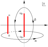
      Figure 4.15. Modulated elliptic wave in the transmission regime: The basis $\{\upalpha,\upbeta\}$ of cycles for the genus-1 Riemann surface associated with the function $\Gamma(\xi,k)$. The cycle $\upbeta$ is a closed, anti-clockwise contour that encircles the branch cut $B$ while lying on the first sheet of the Riemann surface. The cycle $\upalpha$ consists of an anti-clockwise contour that begins from the left of the branch cut $B^{\prime}$ and approaches the branch cut $B$ from the right while lying on the first sheet, and then returns to $B^{\prime}$ via the second sheet (dashed portion).

      Starting from the reconstruction formula (3.13) and applying the successive deformations that lead from $N=N^{(0)}$ to $\widetilde{N}^{(7)}$ while keeping in mind that $n,d,\delta\to 1$ as $k\to\infty$, we obtain

      $$q(x,t)=-2i\lim_{k\to\infty}k\widetilde{N}^{(7)}_{12}(x,t,k)e^{i\left[g_{\infty}(\xi)+\widetilde{g}_{\infty}-G_{\infty}(\xi)t\right]}.$$ (4.75hvij)

      Furthermore, according to the decomposition (4.75hr), for large $k$ we have

      $$\widetilde{N}^{(7)}_{12}=\widetilde{N}_{11}^{\textnormal{err}}\widetilde{N}_{12}^{\textnormal{dom}}+\widetilde{N}_{12}^{\textnormal{err}}\widetilde{N}_{22}^{\textnormal{dom}}.$$ (4.75hvik)

      Hence, using also the asymptotic conditions (4.75htc) and (4.75hva), we find

      $$q(x,t)=-2i\lim_{k\to\infty}k\widetilde{N}_{12}^{\textnormal{dom}}(x,t,k)e^{i\left[g_{\infty}(\xi)+\widetilde{g}_{\infty}-G_{\infty}(\xi)t\right]}-2i\lim_{k\to\infty}k\widetilde{N}_{12}^{\textnormal{err}}(x,t,k).$$ (4.75hvil)

      All of the jumps of $\widetilde{N}^{\textnormal{err}}$, including those along $\partial D_{p}^{\varepsilon}$ and $\partial D_{\bar{p}}^{\varepsilon}$, tend to the identity exponentially fast as $t\to\infty$. Hence, the second term in (4.75hvil) is of lower order. In fact, similarly to [BM2] (see also [BV]) we have

      $$\lim_{k\to\infty}k\widetilde{N}_{12}^{\textnormal{err}}(x,t,k)=O\big{(}t^{-\frac{1}{2}}\big{)},\quad t\to\infty.$$ (4.75hvim)

      Moreover, since the original and deformed versions of $\widetilde{N}^{\textnormal{dom}}$ agree outside the finite region $\mathcal{D}$ enclosed by $\widetilde{B}$ and $B^{\prime}$ (see Figure 4.14) and hence in the limit $k\to\infty$, formula (4.75hvhy) together with the expansion

      $$\eta(\xi,k)=1-\frac{i(q_{o}+\alpha_{\textnormal{im}})}{2k}+O\left(\frac{1}{k^{2}}\right),\quad k\to\infty,$$ (4.75hvin)

      imply

      $$\lim_{k\to\infty}k\widetilde{N}_{12}^{\textnormal{dom}}(x,t,k)=\frac{1}{2}\left(q_{o}+\alpha_{\textnormal{im}}\right)\frac{{\mathbf{\widetilde{N}}}_{2}(\xi,\infty,c)}{{\mathbf{\widetilde{N}}}_{1}(\xi,\infty,c)}\,e^{i\left[g_{\infty}(\xi)+\widetilde{g}_{\infty}-G_{\infty}(\xi)t\right]}.$$ (4.75hvio)

      Therefore, at leading order the reconstruction formula (4.75hvil) yields the modulated elliptic wave

      $$q(x,t)=\frac{q_{o}\left(q_{o}+\alpha_{\textnormal{im}}\right)}{\bar{q}_{-}}\frac{\Theta\big{(}\!-\frac{\Omega t}{2\pi}+\frac{\omega+\widetilde{\omega}}{2\pi}+\frac{i\ln\left(\frac{\bar{q}_{-}}{iq_{o}}\right)}{2\pi}-\upnu_{\infty}+c\big{)}\,\Theta\left(\upnu_{\infty}+c\right)}{\Theta\big{(}\!-\frac{\Omega t}{2\pi}+\frac{\omega+\widetilde{\omega}}{2\pi}+\frac{i\ln\left(\frac{\bar{q}_{-}}{iq_{o}}\right)}{2\pi}+\upnu_{\infty}+c\big{)}\,\Theta\left(-\upnu_{\infty}+c\right)}\,e^{2i\left[g_{\infty}(\xi)+\widetilde{g}_{\infty}-G_{\infty}(\xi)t\right]}\\ +O\big{(}t^{-\frac{1}{2}}\big{)},\quad t\to\infty,$$ (4.75hvip)

      where the real quantities $\alpha_{\textnormal{im}}$, $\Omega$, $\omega$, $\widetilde{\omega}$, $G_{\infty}$, $g_{\infty}$, depend only on $\xi$ and are given respectively by (2.8), (4.75fk), (4.75gs), (4.75hi), (4.75go), (4.75gw), the real constant $\widetilde{g}_{\infty}$ is given by (4.75hm), and the quantities $c(\xi)$ and $\upnu_{\infty}(\xi)$ are defined by (4.75hvih) and (4.75hvii) respectively. In fact, as shown in [BM2], $\Omega$ can be expressed as

      $$\Omega(\xi)=\frac{\pi\left|\alpha+iq_{o}\right|}{K(m)}\left(\xi-2\alpha_{\textnormal{re}}\right)$$ (4.75hviq)

      with $K(m)$ being the complete elliptic integral of the first kind with elliptic modulus $m$ obtained via the modulation equations (2.8). Then, performing some straightforward manipulations of the relevant theta functions, we can write (4.75hvip) in the more explicit form (2.19)-(2.20) with

      $$X_{o}=X_{o}(\xi):=\frac{1}{2\pi}\left[\omega(\xi)-i\ln\Big{(}\frac{q_{-}}{q_{o}}\Big{)}\right]+\frac{1}{4}.$$ (4.75hvir)

      The proof of Theorem 2.1 for the leading-order asymptotics in the transmission regime $p\in D_{1}$ is complete.

      Remark 4.5 (Phase and position shifts).

      Setting $\widetilde{\omega}=\widetilde{g}_{\infty}=0$ in (2.19)-(2.20) gives (2.22), which is precisely the modulated elliptic wave of [BM2]. That is, the effect of the soliton arising at $\xi=v_{s}$ on the leading-order asymptotics for $\xi\in(v_{o},0)$ is the constant phase shift $2\widetilde{g}_{\infty}=4\text{arg}\left[p+\lambda(p)\right]$ as well as a position shift related to the presence of the quantity $\widetilde{\omega}$.

      5. The Trap Regime: Proof of Theorem 2.2

      This regime arises for $p$ inside the region $D_{2}^{+}$ of Figure 2.1. In that case, we have $v_{s}>v_{o}$ i.e. $\text{Re}(i\theta)(\xi,p)<0$ throughout the interval $(-\infty,v_{o})$ and hence no soliton arises there. Furthermore, as already noted in the context of the fifth deformation of Subsection 4.4, for $p\in D_{2}^{+}$ the equation $\text{Re}(ih)(\xi,p)=0$ has a unique solution $\widetilde{v}_{s}$ in the interval $(v_{o},0)$ (in fact, it turns out that $\widetilde{v}_{s}>v_{s}$). Thus, we split the range $(-\infty,0)$ into the subintervals $\xi<v_{o}$; $v_{o}<\xi<\widetilde{v}_{s}$; $\xi=\widetilde{v}_{s}$; and $\widetilde{v}_{s}<\xi<0$.

      5.1. The range $\xi<v_{o}$: plane wave

      No soliton arises in this range since the asymptotics is dictated by the phase function $\theta$ and the fact that $v_{o}<v_{s}$ means that $\text{Re}(i\theta)(\xi,p)<0$ throughout $(-\infty,v_{o})$. Therefore, the analysis required is the same with the one carried out for $\xi<v_{s}$ in the transmission regime (see Subsection 4.1) and the leading-order asymptotics is given by the plane wave (2.14).

      5.2. The range $v_{o}<\xi<\widetilde{v}_{s}$: modulated elliptic wave

      This range is very similar to the range $(v_{o},0)$ of the transmission regime. In particular, applying the first six deformations of Subsection 4.4 we arrive again at Riemann-Hilbert problem (4.75gx) for the function $N^{(6)}$. For $p\in D_{2}^{+}$, however, $\mathop{\rm Re}(ih)(\xi,p)<0$ as opposed to $\mathop{\rm Re}(ih)(\xi,p)>0$ (see Figure 5.1 and the relevant discussion in Subsection 4.4). Therefore, the jumps along $\partial D_{p}^{\varepsilon}$ and $\partial D_{\bar{p}}^{\varepsilon}$ now tend to the identity exponentially fast as $t\to\infty$, allowing us to proceed to the decomposition of problem (4.75gx) into dominant and error components directly, without the need for transformations (4.75hb) and (4.75hg).

      

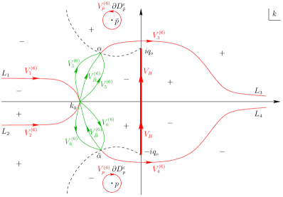
      Figure 5.1. Modulated elliptic wave in the trap regime: the jumps of Riemann-Hilbert problem (4.75gx). Contrary to the corresponding region in the transmission regime, the jumps along $\partial D_{p}^{\varepsilon}$ and $\partial D_{\bar{p}}^{\varepsilon}$ tend to the identity as $t\to\infty$.

      Indeed, performing the analogue of decomposition (4.75hr) and proceeding as in Subsection 4.4, we find

      $$q(x,t)=-2i\lim_{k\to\infty}kN_{12}^{\textnormal{dom}}(x,t,k)e^{i\left[g_{\infty}(\xi)-G_{\infty}(\xi)t\right]}+O\big{(}t^{-\frac{1}{2}}\big{)},$$ (4.75hva)

      where $N^{\textnormal{dom}}$ denotes the solution of the dominant component of Riemann-Hilbert problem (4.75gx) in the case $p\in D_{2}^{+}$. Specifically, as expected from the discussion above, $N^{\textnormal{dom}}$ satisfies problem (4.75ht) with $\widetilde{\omega}=\widetilde{g}_{\infty}=0$, i.e. $N^{\textnormal{dom}}$ is analytic in $\mathbb{C}\setminus(B\cup\widetilde{B})$ with

      $$N^{{\textnormal{dom}}+} =N^{{\textnormal{dom}}-}V_{B}, k\in B,$$ (4.75hvba)

      $$N^{{\textnormal{dom}}+} =N^{{\textnormal{dom}}-}V_{\widetilde{B}}^{(6)}, k\in\widetilde{B},$$ (4.75hvbb)

      $$N^{\textnormal{dom}} =\left[I+O\left(\tfrac{1}{k}\right)\right]e^{i\left[g_{\infty}(\xi)-G_{\infty}(\xi)t\right]\sigma_{3}},\quad k\to\infty.$$ (4.75hvbc)

      Problem (4.75hvb) arises in the case of empty discrete spectrum analyzed in [BM2]. Actually, thanks to the fact that the jump $V_{\widetilde{B}}^{(6)}$ is independent of $k$, the jump contour $\widetilde{B}$ in problem (4.75hvb) can be deformed to the straight line segment $B^{\prime}$ from $\bar{\alpha}$ to $\alpha$ (see Figure 4.14). Then, following [BM2], we obtain the solution of this deformed problem as

      $$N^{\textnormal{dom}}(x,t,k)=e^{i\left[g_{\infty}(\xi)-G_{\infty}(\xi)t\right]\sigma_{3}}\mathcal{N}^{-1}(\xi,\infty,c)\,\mathcal{N}(\xi,k,c),$$ (4.75hvc)

      where

      $$\mathcal{N}(\xi,k,c)=\frac{1}{2}\left(\begin{array}[]{lr}\left[\eta(\xi,k)+\eta^{-1}(\xi,k)\right]{\mathbf{N}}_{1}(\xi,k,c)&i\left[\eta(\xi,k)-\eta^{-1}(\xi,k)\right]{\mathbf{N}}_{2}(\xi,k,c)\\ -i\left[\eta(\xi,k)-\eta^{-1}(\xi,k)\right]{\mathbf{N}}_{1}(\xi,k,-c)&\left[\eta(\xi,k)+\eta^{-1}(\xi,k)\right]{\mathbf{N}}_{2}(\xi,k,-c)\end{array}\right)$$ (4.75hvd)

      and

      $$\mathcal{N}(\xi,\infty,c):=\lim_{k\to\infty}\mathcal{N}(\xi,k,c)$$ (4.75hve)

      with the function $\eta$ defined by (4.75hvib) and with ${\mathbf{N}}_{1}$ and ${\mathbf{N}}_{2}$ denoting the first and second column of the vector-valued function

      $${\mathbf{N}}(\xi,k,c)=\left(\frac{\Theta\big{(}-\frac{\Omega t}{2\pi}+\frac{\omega}{2\pi}+\frac{i\ln\left(\frac{\bar{q}_{-}}{iq_{o}}\right)}{2\pi}+\upnu(k)+c\big{)}}{\sqrt{\frac{iq_{o}}{\bar{q}_{-}}}\ \Theta\left(\upnu(k)+c\right)},\frac{\Theta\big{(}-\frac{\Omega t}{2\pi}+\frac{\omega}{2\pi}+\frac{i\ln\left(\frac{\bar{q}_{-}}{iq_{o}}\right)}{2\pi}-\upnu(k)+c\big{)}}{\sqrt{\tfrac{\bar{q}_{-}}{iq_{o}}}\ \Theta\left(-\upnu(k)+c\right)}\right),$$ (4.75hvf)

      where $\Omega$, $\omega$, $\upnu$ and $c$ are given by (4.75hviq), (4.75gs), (4.75hvig) and (4.75hvih) respectively. We note that formula (4.75hvc) is consistent with formula (4.75hvhy) after setting $\widetilde{\omega}=\widetilde{g}_{\infty}=0$.

      Recall that the original and deformed versions of $N^{\textnormal{dom}}$ agree outside the finite region $\mathcal{D}$ enclosed by $\widetilde{B}$ and $B^{\prime}$ (see Figure 4.14) and hence in the limit $k\to\infty$. Thus, inserting the solution (4.75hvc) in the reconstruction formula (4.75hva) and utilizing the explicit form (4.75hviq) of $\Omega$ together with the theta functions manipulations performed in [BM2], we obtain the leading-order asymptotics (2.21)-(2.22).

      5.3. The case $\xi=\widetilde{v}_{s}$: soliton on top of a modulated elliptic wave

      Recall that in the trap regime currently under consideration the value $\widetilde{v}_{s}$ is the unique solution of equation (2.12) in the interval $(v_{o},0)$. That is, for $p\in D_{2}^{+}$ the quantities $\mathop{\rm Re}(ih)(\xi,p)$ and $\mathop{\rm Re}(ih)(\xi,\bar{p})$ vanish inside $(v_{o},0)$ only at $\xi=\widetilde{v}_{s}$. In turn, the jumps $V_{p}^{(6)}$ and $V_{\bar{p}}^{(6)}$ given by (4.75gz) become part of the dominant component of Riemann-Hilbert problem (4.75gx) only for $\xi=\widetilde{v}_{s}$. Indeed, as noted earlier${}^{\ref{ds-p-foot}}$ and will be confirmed below, whenever these jumps are part of the dominant problem they are eventually converted to residue conditions at $p$ and $\bar{p}$. Thus, the relevant exponentials reduce to $e^{\pm 2ih(\xi,p)t}$, which for $p\in D_{2}^{+}$ are purely oscillatory (as opposed to growing or decaying) only for $\xi=\widetilde{v}_{s}$. On the other hand, thanks to the global sign structure of $\mathop{\rm Re}(ih)$ (see Figure 5.1) the jumps $V_{j}^{(6)}$ tend to the identity exponentially fast as $t\to\infty$, like in the range $(v_{o},\widetilde{v}_{s})$.

      Following the above remarks, for $\xi=\widetilde{v}_{s}$ we write the solution of problem (4.75gx) as

      $$N^{(6)}=N^{\textnormal{err}}N^{\textnormal{asymp}},$$ (4.75hvg)

      where, for disks $D_{k_{o}}^{\epsilon}$, $D_{\alpha}^{\epsilon}$, $D_{\bar{\alpha}}^{\epsilon}$ of radius $\epsilon$ centered at $k_{o}$, $\alpha$, $\bar{\alpha}$ and such that they do not intersect with each other or with $B\cup\overline{D_{p}^{\varepsilon}}\cup\overline{D_{p}^{\varepsilon}}$, we let

      $$N^{\textnormal{asymp}}=\begin{cases}N^{\textnormal{dom}},&k\in\mathbb{C}\setminus(D_{k_{o}}^{\epsilon}\cup D_{\alpha}^{\epsilon}\cup D_{\bar{\alpha}}^{\epsilon}),\\ N^{D},&k\in D_{k_{o}}^{\epsilon}\cup D_{\alpha}^{\epsilon}\cup D_{\bar{\alpha}}^{\epsilon},\end{cases}$$ (4.75hvh)

      and define the functions $N^{\textnormal{dom}}$, $N^{D}$ and $N^{\textnormal{err}}$ as follows:

      1. $N^{\textnormal{dom}}(\widetilde{v}_{s}t,t,k)$ is analytic in $\mathbb{C}\setminus(B\cup\widetilde{B}\cup\partial D_{p}^{\varepsilon}\cup\partial D_{\bar{p}}^{\varepsilon})$ and satisfies the Riemann-Hilbert problem

         $$N^{{\textnormal{dom}}+} =N^{{\textnormal{dom}}-}V_{B}, k\in B,$$ (4.75hvia)

         $$N^{{\textnormal{dom}}+} =N^{{\textnormal{dom}}-}V_{\widetilde{B}}^{(6)}, k\in\widetilde{B},$$ (4.75hvib)

         $$N^{{\textnormal{dom}}+} =N^{{\textnormal{dom}}-}V_{p}^{(6)}, k\in\partial D_{p}^{\varepsilon},$$ (4.75hvic)

         $$N^{{\textnormal{dom}}+} =N^{{\textnormal{dom}}-}V_{\bar{p}}^{(6)}, k\in\partial D_{\bar{p}}^{\varepsilon},$$ (4.75hvid)

         $$N^{\textnormal{dom}} =\left[I+O\left(\tfrac{1}{k}\right)\right]e^{i\left[g_{\infty}(\widetilde{v}_{s})-G_{\infty}(\widetilde{v}_{s})t\right]\sigma_{3}},\quad k\to\infty.$$ (4.75hvie)

      2. $N^{D}(\widetilde{v}_{s}t,t,k)$ is analytic in $D_{k_{o}}^{\epsilon}\cup D_{\alpha}^{\epsilon}\cup D_{\bar{\alpha}}^{\epsilon}\setminus\bigcup_{j=1}^{8}L_{j}$ with jumps

         $$N^{D+}=N^{D-}V_{j}^{(6)},\quad k\in\widehat{L}_{j}:=L_{j}\cap\left(D_{k_{o}}^{\epsilon}\cup D_{\alpha}^{\epsilon}\cup D_{\bar{\alpha}}^{\epsilon}\right),\ j=1,\ldots,8,$$ (4.75hvj)

         as shown in Figure 5.2.

      3. $N^{\textnormal{err}}(\widetilde{v}_{s}t,t,k)$ is analytic in $\mathbb{C}\setminus\big{(}\bigcup_{j=1}^{6}\savestack{\tmpbox}{\stretchto{\scaleto{\scalerel*[width("L")]{\kern-0.6pt\bigwedge\kern-0.6pt}{\rule[-505.89pt]{4.30554pt}{505.89pt}}}{}}{0.5ex}}\stackon[1pt]{L}{\scalebox{-1.0}{\tmpbox}}_{j}\cup\partial D_{k_{o}}^{\epsilon}\cup\partial D_{\alpha}^{\epsilon}\cup\partial D_{\bar{\alpha}}^{\epsilon}\big{)}$ with $\savestack{\tmpbox}{\stretchto{\scaleto{\scalerel*[width("L")]{\kern-0.6pt\bigwedge\kern-0.6pt}{\rule[-505.89pt]{4.30554pt}{505.89pt}}}{}}{0.5ex}}\stackon[1pt]{L}{\scalebox{-1.0}{\tmpbox}}_{j}:=L_{j}\setminus(\overline{D_{k_{o}}^{\epsilon}}\cup\overline{D_{\alpha}^{\epsilon}}\cup\overline{D_{\bar{\alpha}}^{\epsilon}})$ and satisfies the Riemann-Hilbert problem

         $$N^{{\textnormal{err}}+} =N^{{\textnormal{err}}-}\,V^{\textnormal{err}},\quad k\in{\textstyle\bigcup}_{j=1}^{6}\savestack{\tmpbox}{\stretchto{\scaleto{\scalerel*[width("L")]{\kern-0.6pt\bigwedge\kern-0.6pt}{\rule[-505.89pt]{4.30554pt}{505.89pt}}}{}}{0.5ex}}\stackon[1pt]{L}{\scalebox{-1.0}{\tmpbox}}_{j}\cup\partial D_{k_{o}}^{\epsilon}\cup\partial D_{\alpha}^{\epsilon}\cup\partial D_{\bar{\alpha}}^{\epsilon}$$

         $$N^{\textnormal{err}} =I+O\left(\tfrac{1}{k}\right), k\to\infty,$$ (4.75hvka)

         with

         $$V^{\textnormal{err}}=\begin{cases}N^{\textnormal{dom}}V_{j}^{(6)}(N^{\textnormal{dom}})^{-1},&k\in\savestack{\tmpbox}{\stretchto{\scaleto{\scalerel*[width("L")]{\kern-0.6pt\bigwedge\kern-0.6pt}{\rule[-505.89pt]{4.30554pt}{505.89pt}}}{}}{0.5ex}}\stackon[1pt]{L}{\scalebox{-1.0}{\tmpbox}}_{j},\\ N^{{\textnormal{asymp}}-}(V_{D}^{\textnormal{asymp}})^{-1}(N^{{\textnormal{asymp}}-})^{-1},&k\in\partial D_{k_{o}}^{\epsilon}\cup\partial D_{\alpha}^{\epsilon}\cup\partial D_{\bar{\alpha}}^{\epsilon},\end{cases}$$ (4.75hvkl)

         and

         $$V_{D}^{\textnormal{asymp}}=\begin{cases}V_{D_{\alpha}}^{\textnormal{asymp}},&k\in\partial D_{\alpha}^{\epsilon},\\ V_{D_{\bar{\alpha}}}^{\textnormal{asymp}},&k\in\partial D_{\bar{\alpha}}^{\epsilon},\\ V_{D_{k_{o}}}^{\textnormal{asymp}},&k\in\partial D_{k_{o}}^{\epsilon}.\end{cases}$$ (4.75hvkm)

         

         

         

         Figure 5.2. Modulated elliptic wave in the trap regime: The jumps of $N^{D}$ in the interior of and along the boundary of the disks $\overline{D_{\alpha}^{\epsilon}}$, $\overline{D_{\bar{\alpha}}^{\epsilon}}$ and $\overline{D_{k_{o}}^{\epsilon}}$. Although the jumps $V_{D_{\alpha}}^{\textnormal{asymp}}$, $V_{D_{\bar{\alpha}}}^{\textnormal{asymp}}$, $V_{D_{k_{o}}}^{\textnormal{asymp}}$ are unknown, they are equal to the identity up to $O(t^{-1/2})$ and hence do not affect the dominant problem.

         Although $V_{D}^{\textnormal{asymp}}$ is unknown, in [BM2] it was shown that the contribution of the error problem (4.75hvk) to the leading-order asymptotics is of $O\big{(}t^{-1/2}\big{)}$. Therefore, starting from the reconstruction formula (3.13) and applying the six deformations that lead to $N^{(6)}$, we find

         $$q(x,t)=-2i\lim_{k\to\infty}kN_{12}^{\textnormal{dom}}(\widetilde{v}_{s}t,t,k)e^{i\left[g_{\infty}(\widetilde{v}_{s})-G_{\infty}(\widetilde{v}_{s})t\right]}+O\big{(}t^{-\frac{1}{2}}\big{)},\quad t\to\infty.$$ (4.75hvkn)

         It remains to determine $N^{\textnormal{dom}}$.

         Solution of the dominant problem. We now determine the solution $N^{\textnormal{dom}}$ of problem (4.75hvi) via the same series of steps followed in Subsection 4.2. First, we convert the jumps $V_{p}^{(6)}$ and $V_{\bar{p}}^{(6)}$ along the circles $\partial D_{p}^{\varepsilon}$ and $\partial D_{\bar{p}}^{\varepsilon}$ to residue conditions at $p$ and $\bar{p}$ via the transformation

         $$M^{\textnormal{dom}}=\begin{cases}N^{\textnormal{dom}}\big{(}V_{p}^{(6)}\big{)}^{-1},&k\in D_{p}^{\varepsilon},\\ N^{\textnormal{dom}},&k\in\mathbb{C}^{-}\setminus\big{(}B^{-}\cup\widetilde{B}^{-}\cup\overline{D_{p}^{\varepsilon}}\,\big{)},\\ N^{\textnormal{dom}}\big{(}V_{\bar{p}}^{(6)}\big{)}^{-1},&k\in D_{\bar{p}}^{\varepsilon},\\ N^{\textnormal{dom}},&k\in\mathbb{C}^{+}\setminus\big{(}B^{+}\cup\widetilde{B}^{+}\cup\overline{D_{\bar{p}}^{\varepsilon}}\,\big{)}.\end{cases}$$ (4.75hvko)

         Indeed, the function $M^{\textnormal{dom}}$ maintains the jumps of $N^{\textnormal{dom}}$ along $B$ and $\widetilde{B}$ but has simple poles at $p$ and $\bar{p}$ instead of jumps along $\partial D_{p}^{\varepsilon}$ and $\partial D_{\bar{p}}^{\varepsilon}$. Specifically, $M^{\textnormal{dom}}$ satisfies the Riemann-Hilbert problem

         $$M^{{\textnormal{dom}}+}=M^{{\textnormal{dom}}-}V_{B}, k\in B,$$ (4.75hvkpa)

         $$M^{{\textnormal{dom}}+}=M^{{\textnormal{dom}}-}V_{\widetilde{B}}^{(6)}, k\in\widetilde{B},$$ (4.75hvkpb)

         $$M^{\textnormal{dom}}=\left[I+O\left(\tfrac{1}{k}\right)\right]e^{i\left[g_{\infty}(\widetilde{v}_{s})-G_{\infty}(\widetilde{v}_{s})t\right]\sigma_{3}},\quad k\to\infty,$$ (4.75hvkpc)

         $$\underset{k=p}{\text{Res}}\,M^{\textnormal{dom}}=\left(0,\rho_{p}\,M_{1}^{\textnormal{dom}}(p)\right),$$ (4.75hvkpd)

         $$\underset{k=\bar{p}}{\text{Res}}\,M^{\textnormal{dom}}=\left(\rho_{\bar{p}}\,M_{2}^{\textnormal{dom}}(\bar{p}),0\right),$$ (4.75hvkpe)

         where $M_{1}^{\textnormal{dom}},M_{2}^{\textnormal{dom}}$ denote the first and second column of the matrix $M^{\textnormal{dom}}$ and

         $$\rho_{p}=c_{p}\delta^{2}(\widetilde{v}_{s},p)d(p)e^{2i\left[h(\widetilde{v}_{s},p)t-g(\widetilde{v}_{s},p)\right]},$$ (4.75hvkqa)

         $$\rho_{\bar{p}}=c_{\bar{p}}\delta^{-2}(\widetilde{v}_{s},\bar{p})d(\bar{p})e^{-2i\left[h(\widetilde{v}_{s},\bar{p})t-g(\widetilde{v}_{s},\bar{p})\right]}.$$ (4.75hvkqb)

         In fact, similarly to Subsection 4.2, we can use the definitions (3.11a) and (3.11b) of $c_{p}$ and $c_{\bar{p}}$ together with the symmetries $C_{\bar{p}}=-\overline{C_{p}}$, $d(\bar{k})=\overline{d(k)}$, $\bar{a}^{\prime}(\bar{k})=\overline{a^{\prime}(k)}$, $\delta(\xi,\bar{k})=\overline{\delta^{-1}(\xi,k)}$, $g(\xi,\bar{k})=\overline{g(\xi,k)}$, $h(\xi,\bar{k})=\overline{h(\xi,k)}$ and the fact that $h(\widetilde{v}_{s},\bar{p})\in\mathbb{R}$ to write expressions (4.75hvkq) as

         $$\rho_{p}=R_{p}\,e^{2ih(\widetilde{v}_{s},p)t},\quad\rho_{\bar{p}}=-\overline{R_{p}}\,e^{-2ih(\widetilde{v}_{s},p)t},\quad R_{p}:=C_{p}\frac{\delta^{2}(\widetilde{v}_{s},p)e^{-2ig(\widetilde{v}_{s},p)}}{a^{\prime}(p)}.$$ (4.75hvkr)

         Note that the writing (4.75hvkr) reveals that $\rho_{\bar{p}}=-\overline{\rho_{p}}$.

         In order to solve problem (4.75hvkp), it is convenient to let

         $$M^{\textnormal{dom}}=\mathcal{M}^{\textnormal{dom}}W$$ (4.75hvks)

         with $W$ being the solution of the continuous spectrum component problem

         $$W^{+} =W^{-}V_{B}, k\in B,$$ (4.75hvkta)

         $$W^{+} =W^{-}V_{\widetilde{B}}^{(6)}, k\in\widetilde{B},$$ (4.75hvktb)

         $$W =\left[I+O\left(\tfrac{1}{k}\right)\right]e^{i\left[g_{\infty}(\widetilde{v}_{s})-G_{\infty}(\widetilde{v}_{s})t\right]\sigma_{3}},\quad k\to\infty.$$ (4.75hvktc)

         Observe that problem (4.75hvkt) is simply problem (4.75hvb) evaluated at $\xi=\widetilde{v}_{s}$. Therefore, as for problem (4.75hvb), its jump contour $\widetilde{B}$ in problem (4.75hvkt) can be deformed to the straight line segment $B^{\prime}$ connecting $\bar{\alpha}$ with $\alpha$ (see Figure 4.14), and the solution of this deformed problem is given by formula (4.75hvc) as

         $$W=e^{i\left[g_{\infty}(\widetilde{v}_{s})-G_{\infty}(\widetilde{v}_{s})t\right]\sigma_{3}}\mathcal{N}^{-1}(\widetilde{v}_{s},\infty,c)\,\mathcal{N}(\widetilde{v}_{s},k,c)$$ (4.75hvku)

         with $\mathcal{N}$ defined by (4.75hvd). Note further that $\det W$ inherits the analyticity of $W$ away from $B$ and $\widetilde{B}$, while (4.75hvkt) implies that

         $$\det W^{+} =\det W^{-}\det V_{B}, k\in B,$$

         $$\det W^{+} =\det W^{-}\det V_{\widetilde{B}}^{(6)},\quad k\in\widetilde{B}.$$

         Therefore, since $\det V_{B}\equiv\det V_{\widetilde{B}}^{(6)}\equiv 1$, we deduce that $\det W$ does not have jumps along $B$ and $\widetilde{B}$, i.e. $\det W$ is entire in $k$. Moreover, the asymptotic condition (4.75hvktc) implies that $\lim_{k\to\infty}\det W=1$. Thus, we conclude via Liouville’s theorem that $\det W=1$ for all $k\in\mathbb{C}$.

         Combining (4.75hvks) and (4.75hvkt), we find that the discrete component $\mathcal{M}^{\textnormal{dom}}$ of $M^{\textnormal{dom}}$ is analytic in $\mathbb{C}\setminus\left\{p,\bar{p}\right\}$ and has simple poles at $p$ and $\bar{p}$ with the following residues:

         $$\underset{k=p}{\text{Res}}\,\mathcal{M}_{1}^{\textnormal{dom}} =-W_{21}(p)\rho_{p}\,M_{1}^{\textnormal{dom}}(p),$$ (4.75hvkva)

         $$\underset{k=p}{\text{Res}}\,\mathcal{M}_{2}^{\textnormal{dom}} =W_{11}(p)\rho_{p}\,M_{1}^{\textnormal{dom}}(p),$$ (4.75hvkvb)

         $$\underset{k=\bar{p}}{\text{Res}}\,\mathcal{M}_{1}^{\textnormal{dom}} =W_{22}(\bar{p})\rho_{\bar{p}}\,M_{2}^{\textnormal{dom}}(\bar{p}),$$ (4.75hvkvc)

         $$\underset{k=\bar{p}}{\text{Res}}\,\mathcal{M}_{2}^{\textnormal{dom}} =-W_{12}(\bar{p})\rho_{\bar{p}}\,M_{2}^{\textnormal{dom}}(\bar{p}).$$ (4.75hvkvd)

         Moreover, $\mathcal{M}^{\textnormal{dom}}$ satisfies the asymptotic condition

         $$\mathcal{M}^{\textnormal{dom}}=I+O\left(\tfrac{1}{k}\right),\quad k\to\infty.$$ (4.75hvkw)

         Then, arguing as in Subsection 4.2, we deduce that

         $$\mathcal{M}^{\textnormal{dom}}=I+\frac{\underset{k=p}{\text{Res}}\,\mathcal{M}^{\textnormal{dom}}}{k-p}+\frac{\underset{k=\bar{p}}{\text{Res}}\,\mathcal{M}^{\textnormal{dom}}}{k-\bar{p}}.$$ (4.75hvkx)

         Thus, in order to determine $\mathcal{M}^{\textnormal{dom}}$ it suffices to determine its two residues at $p$ and $\bar{p}$.

         From (4.75hvks) we have

         $$M_{1}^{\textnormal{dom}} =W_{1}+W_{11}\left[-\frac{W_{21}(p)\,\rho_{p}\,M_{1}^{\textnormal{dom}}(p)}{k-p}+\frac{W_{22}(\bar{p})\,\rho_{\bar{p}}\,M_{2}^{\textnormal{dom}}(\bar{p})}{k-\bar{p}}\right]$$

         $$\quad+W_{21}\left[\frac{W_{11}(p)\,\rho_{p}\,M_{1}^{\textnormal{dom}}(p)}{k-p}-\frac{W_{12}(\bar{p})\,\rho_{\bar{p}}\,M_{2}^{\textnormal{dom}}(\bar{p})}{k-\bar{p}}\right]$$ (4.75hvkya)

         and

         $$M_{2}^{\textnormal{dom}} =W_{2}+W_{12}\left[-\frac{W_{21}(p)\,\rho_{p}\,M_{1}^{\textnormal{dom}}(p)}{k-p}+\frac{W_{22}(\bar{p})\,\rho_{\bar{p}}\,M_{2}^{\textnormal{dom}}(\bar{p})}{k-\bar{p}}\right]$$

         $$\quad+W_{22}\left[\frac{W_{11}(p)\,\rho_{p}\,M_{1}^{\textnormal{dom}}(p)}{k-p}-\frac{W_{12}(\bar{p})\,\rho_{\bar{p}}\,M_{2}^{\textnormal{dom}}(\bar{p})}{k-\bar{p}}\right].$$ (4.75hvkyb)

         Evaluating the first of the above equations at $k=p$ and the second one at $k=\bar{p}$ (recall that $M_{1}^{\textnormal{dom}}$ and $M_{2}^{\textnormal{dom}}$ are analytic at $p$ and $\bar{p}$ respectively), we obtain the system

         $$M_{1}^{\textnormal{dom}}(p) =W_{1}(p)+\rho_{\bar{p}}\,\frac{W_{11}(p)W_{22}(\bar{p})-W_{21}(p)W_{12}(\bar{p})}{p-\bar{p}}\,M_{2}^{\textnormal{dom}}(\bar{p})$$

         $$\quad+\rho_{p}\left[W_{21}^{\prime}(p)W_{11}(p)-W_{11}^{\prime}(p)W_{21}(p)\right]M_{1}^{\textnormal{dom}}(p),$$ (4.75hvkza)

         $$M_{2}^{\textnormal{dom}}(\bar{p}) =W_{2}(\bar{p})+\rho_{p}\,\frac{W_{12}(\bar{p})W_{21}(p)-W_{22}(\bar{p})W_{11}(p)}{p-\bar{p}}\,M_{1}^{\textnormal{dom}}(p)$$

         $$\quad+\rho_{\bar{p}}\left[W_{12}^{\prime}(\bar{p})W_{22}(\bar{p})-W_{22}^{\prime}(\bar{p})W_{12}(\bar{p})\right]M_{2}^{\textnormal{dom}}(\bar{p}),$$ (4.75hvkzb)

         which can be solved to yield

         $$M_{1}^{\textnormal{dom}}(p) =\frac{-\mathcal{B}\rho_{\bar{p}}W_{2}(\bar{p})+\left(1+\mathcal{C}\rho_{\bar{p}}\right)W_{1}(p)}{\mathcal{B}^{2}\rho_{p}\rho_{\bar{p}}+\left(1+\mathcal{C}\rho_{\bar{p}}\right)\left(1+\mathcal{A}\rho_{p}\right)},$$ (4.75hvkaaa)

         $$M_{2}^{\textnormal{dom}}(\bar{p}) =\frac{\mathcal{B}\rho_{p}W_{1}(p)+\left(1+\mathcal{A}\rho_{p}\right)W_{2}(\bar{p})}{\mathcal{B}^{2}\rho_{p}\rho_{\bar{p}}+\left(1+\mathcal{C}\rho_{\bar{p}}\right)\left(1+\mathcal{A}\rho_{p}\right)},$$ (4.75hvkaab)

         where

         $$\mathcal{A} =W_{11}^{\prime}(p)W_{21}(p)-W_{11}(p)W_{21}^{\prime}(p),$$ (4.75hvkaba)

         $$\mathcal{B} =\frac{W_{21}(p)W_{12}(\bar{p})-W_{11}(p)W_{22}(\bar{p})}{p-\bar{p}},$$ (4.75hvkabb)

         $$\mathcal{C} =W_{22}^{\prime}(\bar{p})W_{12}(\bar{p})-W_{12}^{\prime}(\bar{p})W_{22}(\bar{p}).$$ (4.75hvkabc)

         Expressions (4.75hvkaa) determine $\mathcal{M}^{\textnormal{dom}}$ through (4.75hvkx) and the residue relations (4.75hvkv).

         Having computed $\mathcal{M}^{\textnormal{dom}}$, we return to the reconstruction formula (4.75hvkn) which upon (4.75hvko) and (4.75hvks) reads

         $$q(x,t)=-2i\lim_{k\to\infty}k\big{(}\mathcal{M}^{\textnormal{dom}}W\big{)}_{12}e^{i\left[g_{\infty}(\widetilde{v}_{s})-G_{\infty}(\widetilde{v}_{s})t\right]}+O\big{(}t^{-\frac{1}{2}}\big{)},\quad t\to\infty.$$ (4.75hvkac)

         Now, the asymptotic conditions (4.75hvktc) and (4.75hvkw) imply

         $$W=e^{i\left[g_{\infty}(\widetilde{v}_{s})-G_{\infty}(\widetilde{v}_{s})t\right]\sigma_{3}}+\frac{w}{k}+O\left(\frac{1}{k^{2}}\right),\quad\mathcal{M}^{\textnormal{dom}}=I+\frac{\mu}{k}+O\left(\frac{1}{k^{2}}\right),\quad k\to\infty,$$

         where the matrix-valued functions $w$ and $\mu$ may depend on $x$ and $t$ but not on $k$. Therefore,

         $$\big{(}\mathcal{M}^{\textnormal{dom}}W\big{)}_{12}=\frac{w_{12}+\mu_{12}\,e^{-i\left[g_{\infty}(\widetilde{v}_{s})-G_{\infty}(\widetilde{v}_{s})t\right]}}{k}+O\left(\frac{1}{k^{2}}\right),\quad k\to\infty.$$

         Substituting for $w_{12}$ via (4.75hvku) (note that the original and deformed versions of $W$ agree outside the finite region $\mathcal{D}$ enclosed by $\widetilde{B}$ and $B^{\prime}$ in Figure 4.14 and hence as $k\to\infty$) and for $\mu_{12}$ via (4.75hvkv) and (4.75hvkx) yields the leading-order asymptotics (2.23)-(2.24) via the reconstruction formula (4.75hvkac).

         Remark 5.1 (Dependence on $g_{\infty}$ and $G_{\infty}$).

         Formula (4.75hvku) implies that $W_{11}$ and $W_{12}$ depend on $g_{\infty}$ and $G_{\infty}$ through the exponential $e^{i\left[g_{\infty}(\widetilde{v}_{s})-G_{\infty}(\widetilde{v}_{s})t\right]}$ while $W_{21}$ and $W_{22}$ instead contain the exponential $e^{-i\left[g_{\infty}(\widetilde{v}_{s})-G_{\infty}(\widetilde{v}_{s})t\right]}$. Hence, the quantities $\mathcal{A},\mathcal{B},\mathcal{C}$ defined by (4.75hvkab) are independent of $g_{\infty}$ and $G_{\infty}$, and the overall dependence of the leading-order asymptotics (2.23) on $g_{\infty}$ and $G_{\infty}$ comes through a factor of $e^{2i\left[g_{\infty}(\widetilde{v}_{s})-G_{\infty}(\widetilde{v}_{s})t\right]}$.

         5.4. The range $\widetilde{v}_{s}<\xi<0$: modulated elliptic wave with a phase shift

         This range can be handled identically to the range $v_{o}<\xi<0$ of the transmission regime that was analyzed in Subsection 4.4. Consequently, the leading-order asymptotics is characterized once again by (4.75hvip) as the modulated elliptic wave (2.20) with a phase shift of $4\textnormal{arg}\left[p+\lambda(p)\right]$.

         The proof of Theorem 2.2 for the leading-order asymptotics in the trap regime $p\in D_{2}^{+}$ is complete.

         6. The Mixed Regimes: Proof of Theorems 2.3 and 2.4

         In Sections 4 and 5, we showed that the scenarios $p\in D_{1}$ and $p\in D_{2}^{+}$ give rise to pure asymptotic regimes, namely a transmission regime (Theorem 2.1) and a trap regime (Theorem 2.2) respectively. We now proceed to the analysis of the remaining two regions of Figure 2.1, namely $D_{2}^{-}$ and $D_{3}$. We shall show that these regions correspond to mixed asymptotic regimes, specifically a trap/wake regime (Theorem 2.3) and a transmission/wake regime (Theorem 2.4) respectively.

         6.1. The trap/wake regime

         Recall that for $p\in D_{2}^{-}$ we have $v_{o}<v_{s}<0$. Furthermore, as noted in Subsection 4.4, the integral equation (4.75gp) possesses exactly two solutions in the interval $(v_{o},0)$: $\widetilde{v}_{s}$, which corresponds to the crossing of the pole $p$ by the dashed black curve in the third quadrant of Figure 6.1 (for $\xi<\widetilde{v}_{s}$, the pole lies below this curve), and $v_{w}>\widetilde{v}_{s}$, which corresponds to the crossing of $p$ by the branch cut $\widetilde{B}$ (green contour connecting $\alpha$ and $\bar{\alpha}$ in Figure 6.1). Note that the latter crossing can happen only if $p$ lies on the right (as opposed to the left) of $\widetilde{B}$ immediately after $\xi=\widetilde{v}_{s}$, and this is the way one distinguishes the trap/wake regime $p\in D_{2}^{-}$ from the trap regime $p\in D_{2}^{+}$.

         For $\xi<v_{o}$, the deformations performed in the trap regime can be repeated to lead once again to Riemann-Hilbert problem (4.50). Furthermore, like in the trap regime, for $\xi<v_{o}$ the dominant component of this problem only involves the jump along the branch cut $B$ since the jumps along $\partial D_{p}^{\varepsilon}$ and $\partial D_{\bar{p}}^{\varepsilon}$ tend to the identity exponentially fast as $t\to\infty$ due to the fact that $\text{Re}(i\theta)(\xi,p)<0$ and $\text{Re}(i\theta)(\xi,\bar{p})>0$ throughout the interval $(-\infty,v_{o})$. Thus, the leading-order asymptotics for $p\in D_{2}^{-}$ and $\xi\in(-\infty,v_{o})$ is the same with the one of the trap regime, i.e. it is described by the plane wave (2.14).

         For $v_{o}<\xi<\widetilde{v}_{s}$, the phase function switches from $\theta$ to $h$ via transformation (4.75fl) and we eventually arrive at Riemann-Hilbert problem (4.75gx). Moreover, we still have $\text{Re}(ih)(\xi,p)<0$ and $\text{Re}(ih)(\xi,\bar{p})>0$, thus the jumps along $\partial D_{p}^{\varepsilon}$ and $\partial D_{\bar{p}}^{\varepsilon}$ still do not contribute to the leading-order asymptotics, which is described by the modulated elliptic wave (2.22).

         At $\xi=\widetilde{v}_{s}$, we have $\text{Re}(ih)(\widetilde{v}_{s},p)=\text{Re}(ih)(\widetilde{v}_{s},\bar{p})=0$. Thus, as explained in Subsection 5.3, the jumps along $\partial D_{p}^{\varepsilon}$ and $\partial D_{\bar{p}}^{\varepsilon}$ now contribute to the leading-order asymptotics, which is described by (2.23) as the soliton (2.24) on top of the modulated elliptic wave (2.22) evaluated at $\widetilde{v}_{s}$.

         

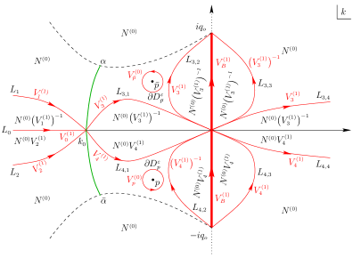
         Figure 6.1. Modulated elliptic wave in the trap/wake ($p\in D_{2}^{-}$) and transmission/wake ($p\in D_{3}$) regimes in the ranges $\widetilde{v}_{s}<\xi<v_{w}$ (for $p\in D_{2}^{-}$) and $v_{o}<\xi<v_{w}$ (for $p\in D_{3}$): the initial stage of the first deformation. The jumps along $\partial D_{p}^{\varepsilon}$ and $\partial D_{\bar{p}}^{\varepsilon}$ are not affected.

         

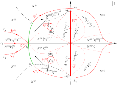
         Figure 6.2. Modulated elliptic wave in the trap/wake ($p\in D_{2}^{-}$) and transmission/wake ($p\in D_{3}$) regimes in the ranges $\widetilde{v}_{s}<\xi<v_{w}$ (for $p\in D_{2}^{-}$) and $v_{o}<\xi<v_{w}$ (for $p\in D_{3}$): the final stage of the first deformation. The jumps along $\partial D_{p}^{\varepsilon}$ and $\partial D_{\bar{p}}^{\varepsilon}$ have now changed.

         The range $\widetilde{v}_{s}<\xi<v_{w}$, which is not present in the trap regime since $v_{w}$ does not arise there, requires a modification of the first four deformations. Specifically, while the first stage of the first deformation remains the same (compare Figure 6.1 with Figure 4.7), the poles $p$ and $\bar{p}$ now lie on the right of the branch cut $\widetilde{B}$. We emphasize that this is the defining difference between the trap/wake regime $p\in D_{2}^{-}$ and the trap regime $p\in D_{2}^{+}$, since in the latter case the poles are always on the left of $\widetilde{B}$ for $\xi>\widetilde{v}_{s}$ (see also Figure 3.3). Thus, for $\widetilde{v}_{s}<\xi<v_{w}$ in the trap/wake regime, in order to lift the jump along $[k_{o},0]$ away from the real axis and onto $\widetilde{B}$, the remaining stages of the first deformation are adjusted from those of the trap regime to the factorization shown in Figure 6.2. Then, applying the second deformation (4.17) with $\delta$ given by (4.75ev) and the third deformation as shown in Figure 4.6 but with the disks $D_{p}^{\varepsilon}$ and $D_{\bar{p}}^{\varepsilon}$ now lying between the contours $L_{3}$ and $L_{4}$, we obtain the analogue of Figure 4.8, the only difference now being that the poles $p$ and $\bar{p}$ lie on the right of $\widetilde{B}$. Subsequently, proceeding as in Subsection 4.4, we eventually arrive at the deformed Riemann-Hilbert problem of Figure 6.3, which can be handled in the same way with Riemann-Hilbert problem (4.75hn). Indeed, since $\text{Re}(ih)(\xi,p)>0$ and $\text{Re}(ih)(\xi,\bar{p})<0$, the jumps along $\partial D_{p}^{\varepsilon}$ and $\partial D_{\bar{p}}^{\varepsilon}$ are not significant at leading order and the corresponding asymptotics is given by (2.19) as the modulated elliptic wave (2.20) with a phase shift of $4\textnormal{arg}\left[p+\lambda(p)\right]$.

         

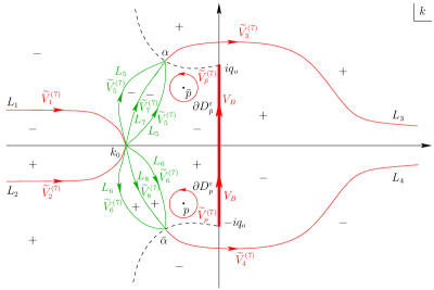
         Figure 6.3. Modulated elliptic wave in the trap/wake ($p\in D_{2}^{-}$) and transmission/wake regimes ($p\in D_{3}$): the jumps of the Riemann-Hilbert problem (4.75hn), the final problem in the ranges $\xi\in(\widetilde{v}_{s},v_{w})\cup(v_{w},0)$ (for $p\in D_{2}^{-}$) and $\xi\in(v_{o},v_{w})\cup(v_{w},0)$ (for $p\in D_{3}$).

         For $v_{w}<\xi<0$, the poles $p$ and $\bar{p}$ lie on the left of $\widetilde{B}$ and, therefore, the analysis is identical to the one for the trap regime in the range $\widetilde{v}_{s}<\xi<0$, leading once again to the asymptotics (2.19).

         It remains to analyze the case $\xi=v_{w}$, which corresponds to the crossing of the poles $p$ and $\bar{p}$ by the branch cut $\widetilde{B}$ of $h$ (green contour connecting $\alpha$ and $\bar{\alpha}$ in Figure 6.1) as the latter sweeps the region to its right en route to collapsing onto $B$ as $\xi\to 0^{-}$. Since $\widetilde{B}$ is also a zero-contour of $\text{Re}(ih)$, this is the mechanism giving rise to the second solution of equation (4.75gp) when $p\in D_{2}^{-}$, since $\text{Re}(ih)(\xi,k)$ vanishes along $\widetilde{B}$ for all $\xi$ and hence $\text{Re}(ih)(v_{w},p)=0$. As previously emphasized, the crossing of $p$ and $\bar{p}$ by $\widetilde{B}$ occurs for $p\in D_{2}^{-}$ but not for $p\in D_{2}^{+}$, since in the latter case the poles are always on the left of $\widetilde{B}$ in the range $\widetilde{v}_{s}<\xi<0$.

         The case $\xi=v_{w}$: soliton wake. For this value of $\xi$, the poles $p$ and $\bar{p}$ lie on $\widetilde{B}$ (depicted in green in Figure 6.1), which is both a zero-contour for $\text{Re}(ih)$ and a branch cut for $h$ (along with the branch cut $B=i[-q_{o},q_{o}]$). For this reason, in view of the fifth deformation of Riemann-Hilbert problem (3.16) (see (4.75fl)), it is convenient to switch from $h$ to a function $h_{w}$ which does not have a branch cut along $\widetilde{B}$ but which is such that $\text{Re}(ih_{w})$ still vanishes along $\widetilde{B}$. More specifically, we define

         $$h_{w}(k)=\left\{\begin{array}[]{ll}h(v_{w},k),&k\in\mathbb{C}\setminus\overline{\mathcal{R}},\\ \Omega(v_{w})-h(v_{w},k),&k\in\mathcal{R},\end{array}\right.$$ (4.75hvka)

         where the real constant $\Omega(v_{w})$ is given by (4.75hviq) and $\mathcal{R}$ is the finite region enclosed by $\widetilde{B}$ and the contour $\widetilde{B}_{w}$ shown in blue in Figure 6.4. It is straightforward to see that the function $h_{w}$ (i) has branch cuts along $B$ and $\widetilde{B}_{w}$, and (ii) is continuous along $\widetilde{B}$. Indeed, recall (see (4.75fjb)) that along $\widetilde{B}$ we have $h^{+}+h^{-}=\Omega(v_{w})$. Hence, according to the definition (4.75hvka) of $h_{w}$, along $\widetilde{B}$ we have $h_{w}^{+}=\left(\Omega(v_{w})-h\right)^{+}=\Omega(v_{w})-h^{+}=h^{-}=h_{w}^{-}$, i.e. $h_{w}$ is continuous along $\widetilde{B}$. On the other hand, along the contour $\widetilde{B}_{w}$ shown in blue in Figure 6.4 we have $h_{w}^{+}=\left(\Omega(v_{w})-h\right)^{+}=\Omega(v_{w})-h=\Omega(v_{w})-h_{w}^{-}$ (having used the fact that $h$ is continuous along $\widetilde{B}_{w}$). Hence, $h_{w}$ is discontinuous along $\widetilde{B}_{w}$ with $h_{w}^{+}+h_{w}^{-}=\Omega(v_{w})$. Furthermore, $h_{w}$ is discontinuous along $B$ since it is equal to $h$ on both sides of $B$. Therefore, $h_{w}$ has branch cuts along $B$ and $\widetilde{B}_{w}$ and is continuous along $\widetilde{B}$.

         

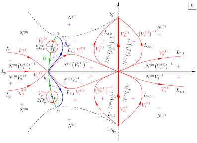
         Figure 6.4. Modulated elliptic wave in the trap/wake ($p\in D_{2}^{-}$) and transmission/wake ($p\in D_{3}$) regimes at $\xi=v_{w}$: the sign structure of $\text{Re}(ih_{w})$ and the initial stage of the first deformation. Note that the jumps along $\partial D_{p}^{\varepsilon}$ and $\partial D_{\bar{p}}^{\varepsilon}$ are not affected. Furthermore, the branch cut $\widetilde{B}_{w}$ of the function $h_{w}$ (blue contour) lies on the right of the zero-contour $\widetilde{B}$ of $\text{Re}(ih_{w})$ (green contour) as well as on the right of the circles $\partial D_{p}^{\varepsilon}$ and $\partial D_{\bar{p}}^{\varepsilon}$. The finite region enclosed by $\widetilde{B}$ and $\widetilde{B}_{w}$ is denoted by $\mathcal{R}$.

         The sign structure of $\text{Re}(ih_{w})$ is shown in Figure 6.4. With this in mind, we perform the first deformation according to Figure 6.4 and then deform the contours $L_{3,1}$, $L_{3,2}$ and $L_{4,1}$, $L_{4,2}$ to the contours $L_{3}$ and $L_{4}$ of Figure 6.5, which depicts the final stage of the first deformation. Note that $L_{3}$ consists of the upper half of the branch cut $\widetilde{B}_{w}$ as well as of the red contour starting from $\alpha$ and curving around $iq_{o}$ and down towards the positive real axis. Similarly, $L_{4}$ consists of both the lower half of $\widetilde{B}_{w}$ and the red curve emanating from $\bar{\alpha}$ and directed upwards towards the positive real axis.

         

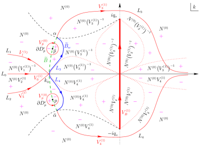
         Figure 6.5. Modulated elliptic wave in the trap/wake ($p\in D_{2}^{-}$) and transmission/wake ($p\in D_{3}$) regimes at $\xi=v_{w}$: the final stage of the first deformation. The jumps along $\partial D_{p}^{\varepsilon}$ and $\partial D_{\bar{p}}^{\varepsilon}$ are not affected.

         The second and third deformations are identical to those performed in the trap regime, leading to Riemann-Hilbert problem (4.75eu) but with the contours $L_{j}$, $j=1,2,3,4$ as shown in Figure 6.5. For the fourth deformation, we use the factorizations (4.75ew) to “open up the lenses” off the portions of the contours $L_{3}$ and $L_{4}$ that lie along $\widetilde{B}_{w}$ as shown in Figure 6.6, where the jumps $V_{j}^{(4)}$, $j=5,6,7,8$ are given by (4.75fb). This figure provides the analogue of Figure 4.9, where the role of the contour $\widetilde{B}$ (which is a branch cut for $h$ and a zero-contour for $\text{Re}(ih)$ and, by definition (4.75hvka), for $\text{Re}(ih_{w})$) is now held by the contour $\widetilde{B}_{w}$ (which is a branch cut for $h_{w}$). The difference between Figures 4.9 and 6.6 is that in the latter case the disks $\overline{D_{p}^{\varepsilon}}$ and $\overline{D_{\bar{p}}^{\varepsilon}}$ lie between the contours $L_{6}$, $L_{8}$ and $L_{5}$, $L_{7}$ respectively. This is necessary in order for the contours $L_{5}$ and $L_{6}$ to lie in regions where the associated jumps $V_{5}^{(4)}$ and $V_{6}^{(4)}$ decay to the identity as $t\to\infty$. Hence, in the fourth deformation shown in Figure 6.6, $N^{(3)}$ changes to $N^{(3)}V_{6}^{(4)}$ in $D_{p}^{\varepsilon}$ and to $N^{(3)}\big{(}V_{5}^{(4)}\big{)}^{-1}$ in $D_{\bar{p}}^{\varepsilon}$ (in Figure 4.9, $N^{(3)}$ remains invariant inside the two disks). Consequently, $N^{(4)}$ satisfies the Riemann-Hilbert problem (4.75fh) but with the jumps along $\partial D_{p}^{\varepsilon}$ and $\partial D_{\bar{p}}^{\varepsilon}$ now given by

         $$V_{p}^{(4)}=\big{(}V_{6}^{(4)}\big{)}^{-1}V_{p}^{(3)}V_{6}^{(4)},\quad V_{\bar{p}}^{(4)}=V_{5}^{(4)}V_{\bar{p}}^{(3)}\big{(}V_{5}^{(4)}\big{)}^{-1},$$ (4.75hvkb)

         where we recall that

         $$V_{p}^{(3)}=\left(\begin{array}[]{lr}1&-\dfrac{c_{p}\,\delta^{2}(v_{w},k)\,d(k)}{k-p}\,e^{2i\theta(v_{w},p)t}\\ 0&1\end{array}\right),\quad V_{\bar{p}}^{(3)}=\left(\begin{array}[]{lr}1&0\\ -\tfrac{c_{\bar{p}}\,\delta^{-2}(v_{w},k)\,d(k)}{k-\bar{p}}\,e^{-2i\theta(v_{w},\bar{p})t}&1\end{array}\right)$$ (4.75hvkc)

         and

         $$V_{5}^{(4)}=\left(\begin{array}[]{lr}1&\tfrac{\delta^{2}}{r}\,e^{2i\theta t}\\ 0&1\end{array}\right),\quad V_{6}^{(4)}=\left(\begin{array}[]{lr}1&0\\ \frac{1}{\bar{r}\delta^{2}}\,e^{-2i\theta t}&1\end{array}\right).$$ (4.75hvkd)

         

         Figure 6.6. Modulated elliptic wave in the trap/wake ($p\in D_{2}^{-}$) and transmission/wake ($p\in D_{3}$) regimes at $\xi=v_{w}$: the fourth deformation. We recall that the dashed green contour is the branch cut $\widetilde{B}$ of $h$, along which $\text{Re}(ih)=\text{Re}(ih_{w})=0$, while the function $h_{w}$ has branch cuts along $B=i[-q_{o},q_{o}]$ and $\widetilde{B}_{w}=L_{7}\cup(-L_{8})$.

         Next, we switch from $N^{(4)}$ to $N^{(5)}$ via the analogue of transformation (4.75fl), now involving $h_{w}$ defined by (4.75hvka) instead of $h$:

         $$N^{(5)}(v_{w}t,t,k)=N^{(4)}(v_{w}t,t,k)e^{-i\left[h_{w}(k)-\theta(v_{w},k)\right]t\sigma_{3}}.$$ (4.75hvke)

         This transformation results in the analogue of Riemann-Hilbert problem (4.75fm), where all relevant jumps are given by (4.75ft) with $h$ replaced by $h_{w}$ except for the jumps along $\partial D_{p}^{\varepsilon}$ and $\partial D_{\bar{p}}^{\varepsilon}$, which are equal to

         $$V_{p}^{(5)} =e^{i\left(h_{w}-\theta\right)t\sigma_{3}}\big{(}V_{6}^{(4)}\big{)}^{-1}V_{p}^{(3)}V_{6}^{(4)}e^{-i\left(h_{w}-\theta\right)t\sigma_{3}},$$ (4.75hvkfa)

         $$V_{\bar{p}}^{(5)} =e^{i\left(h_{w}-\theta\right)t\sigma_{3}}V_{5}^{(4)}V_{\bar{p}}^{(3)}\big{(}V_{5}^{(4)}\big{)}^{-1}e^{-i\left(h_{w}-\theta\right)t\sigma_{3}}.$$ (4.75hvkfb)

         Finally, we perform the sixth deformation similarly to (4.75gq), i.e. we let

         $$N^{(6)}(v_{w}t,t,k)=N^{(5)}(v_{w}t,t,k)e^{ig_{w}(k)\sigma_{3}},$$ (4.75hvkg)

         where the function $g_{w}$, which is the analogue of the function $g$ involved in (4.75gq), is analytic in $\mathbb{C}\setminus(B\cup\widetilde{B}_{w})$ and satisfies the following jump conditions:

         $$g_{w}^{+}+g_{w}^{-} =-i\ln\left(\delta^{2}\right), k\in B,$$ (4.75hvkha)

         $$g_{w}^{+}+g_{w}^{-} =-i\ln\left(\tfrac{\delta^{2}}{r}\right)+\omega_{w},\quad k\in L_{7},$$ (4.75hvkhb)

         $$g_{w}^{+}+g_{w}^{-} =-i\ln\left(\delta^{2}\bar{r}\right)+\omega_{w}, k\in L_{8},$$ (4.75hvkhc)

         with the contours $B$, $L_{7}$, $L_{8}$ as in Figure 6.6, the function $\delta(v_{w},k)$ given by (4.75ev) and the real constant $\omega_{w}$ defined by

         $$\omega_{w}=i\,\frac{\displaystyle\int_{B}\frac{\ln\delta^{2}(v_{w},\nu)}{\gamma_{w}(\nu)}\,d\nu+\int_{\widetilde{B}_{w}^{+}}\frac{\ln\left[\frac{\delta^{2}(v_{w},\nu)}{r(\nu)}\right]}{\gamma_{w}(\nu)}\,d\nu+\int_{\widetilde{B}_{w}^{-}}\frac{\ln\left[\delta^{2}(v_{w},\nu)\,\bar{r}(\nu)\right]}{\gamma_{w}(\nu)}\,d\nu}{\displaystyle\int_{\widetilde{B}_{w}}\frac{d\nu}{\gamma_{w}(\nu)}},$$ (4.75hvki)

         where

         $$\widetilde{B}_{w}^{\pm}:=\widetilde{B}_{w}\cap\mathbb{C}^{\pm}$$ (4.75hvkj)

         and the function $\gamma_{w}$ is defined in terms of the function $\gamma$ (see (2.9)) by

         $$\gamma_{w}(k)=\left\{\begin{array}[]{ll}\gamma(v_{w},k),&k\in\mathbb{C}\setminus\overline{\mathcal{R}},\\ -\gamma(v_{w},k),&k\in\mathcal{R},\end{array}\right.$$ (4.75hvkk)

         where we recall that $\mathcal{R}$ is the finite region enclosed by $\widetilde{B}$ and $\widetilde{B}_{w}$ (see Figure 6.4). Recalling further that $\gamma$ is analytic in $\mathbb{C}\setminus B\cup\widetilde{B}$ and changes sign as $k$ crosses $B$ and $\widetilde{B}$, we deduce that $\gamma_{w}$ has branch cuts along $B$ and $\widetilde{B}_{w}$, across which it changes sign, but is continuous as $k$ crosses $\widetilde{B}$. Dividing the jumps of problem (4.75hvkh) by $\gamma_{w}$ and using Plemelj’s formulae, we obtain

         $$g_{w}(k)=\frac{\gamma_{w}(k)}{2\pi}\bigg{[}\int_{B}\frac{\ln\delta^{2}(v_{w},\nu)}{\gamma_{w}(\nu)(\nu-k)}\,d\nu+\int_{L_{7}}\frac{\ln\left[\frac{\delta^{2}(v_{w},\nu)}{r(\nu)}\right]+i\omega_{w}}{\gamma_{w}(\nu)(\nu-k)}\,d\nu-\int_{L_{8}}\frac{\ln\left[\delta^{2}(v_{w},\nu)\,\bar{r}(\nu)\right]+i\omega_{w}}{\gamma_{w}(\nu)(\nu-k)}\,d\nu\bigg{]}.$$ (4.75hvkl)

         We note that the presence of $\omega_{w}$ in the above formula ensures that $g_{w}(k)=g_{w,\infty}+O\left(\frac{1}{k}\right)$ as $k\to\infty$ with the real constant $g_{w,\infty}$ given by

         $$g_{w,\infty}=-\frac{1}{2\pi}\bigg{[}\int_{B}\frac{\ln\delta^{2}(v_{w},\nu)}{\gamma_{w}(\nu)}\,\nu d\nu+\int_{\widetilde{B}_{w}^{+}}\frac{\ln\left[\frac{\delta^{2}(v_{w},\nu)}{r(\nu)}\right]+i\omega_{w}}{\gamma_{w}(\nu)}\,\nu d\nu+\int_{\widetilde{B}_{w}^{-}}\frac{\ln\left[\delta^{2}(v_{w},\nu)\,\bar{r}(\nu)\right]+i\omega_{w}}{\gamma_{w}(\nu)}\,\nu d\nu\bigg{]}.$$ (4.75hvkm)

         Transformation (4.75hvkg) results in the analogue of Riemann-Hilbert problem (4.75gx), i.e.

         $$N^{(6)+} =N^{(6)-}V_{B}, k\in B,$$ (4.75hvkna)

         $$N^{(6)+} =N^{(6)-}V_{\widetilde{B}_{w}}^{(6)}, k\in\widetilde{B}_{w},$$ (4.75hvknb)

         $$N^{(6)+} =N^{(6)-}V_{j}^{(6)}, k\in L_{j},\ j=1,\ldots,6,$$ (4.75hvknc)

         $$N^{(6)+} =N^{(6)-}V_{p}^{(6)}, k\in\partial D_{p}^{\varepsilon},$$ (4.75hvknd)

         $$N^{(6)+} =N^{(6)-}V_{\bar{p}}^{(6)}, k\in\partial D_{\bar{p}}^{\varepsilon},$$ (4.75hvkne)

         $$N^{(6)} =\left[I+O\left(\tfrac{1}{k}\right)\right]e^{i\left[g_{w,\infty}-G_{\infty}(v_{w})t\right]\sigma_{3}},\quad k\to\infty,$$ (4.75hvknf)

         where the jump along $B$ is given by (4.8), the jump along $\widetilde{B}_{w}$ is equal to

         $$V_{\widetilde{B}_{w}}^{(6)}=\left(\begin{array}[]{lr}0&-e^{i(\Omega(v_{w})t-\omega_{w})}\\ e^{-i(\Omega(v_{w})t-\omega_{w})}&0\end{array}\right)$$ (4.75hvko)

         with the real constants $\Omega(v_{w})$ and $\omega_{w}$ given by (4.75hviq) and (4.75hvki) respectively, the jumps along the contours $L_{j}$ of Figure 6.6 are equal to

         $$V_{1}^{(6)} =\left(\begin{array}[]{lr}1&\frac{\bar{r}\,\delta^{2}e^{-2ig_{w}}}{1+r\bar{r}}\,e^{2ih_{w}t}\\ 0&1\end{array}\right),\quad V_{2}^{(6)}=\left(\begin{array}[]{lr}1&0\\ \frac{r\delta^{-2}e^{2ig_{w}}}{1+r\bar{r}}\,e^{-2ih_{w}t}&1\end{array}\right),$$ (4.75hvkpe)

         $$V_{3}^{(6)} =\left(\begin{array}[]{lr}1&0\\ r\delta^{-2}e^{2ig_{w}}e^{-2ih_{w}t}&1\end{array}\right),\quad V_{4}^{(6)}=\left(\begin{array}[]{lr}1&\bar{r}\delta^{2}e^{-2ig_{w}}e^{2ih_{w}t}\\ 0&1\end{array}\right),$$ (4.75hvkpj)

         $$V_{5}^{(6)} =\left(\begin{array}[]{lr}1&\frac{\delta^{2}e^{-2ig_{w}}}{r}\,e^{2ih_{w}t}\\ 0&1\end{array}\right),\quad V_{6}^{(6)}=\left(\begin{array}[]{lr}1&0\\ \frac{\delta^{-2}e^{2ig_{w}}}{\bar{r}}\,e^{-2ih_{w}t}&1\end{array}\right),$$ (4.75hvkpo)

         the jumps along $\partial D_{p}^{\varepsilon}$ and $\partial D_{\bar{p}}^{\varepsilon}$ are given by

         $$V_{p}^{(6)} =\left(\begin{array}[]{lr}1-\frac{c_{p}d(k)}{\bar{r}(k)\left(k-p\right)}\,e^{-2i\left[\theta(v_{w},k)-\theta(v_{w},p)\right]t}&-\frac{c_{p}\delta^{2}(v_{w},k)d(k)e^{-2ig_{w}(k)}}{k-p}\,e^{2i\left[h_{w}(k)-\theta(v_{w},k)+\theta(v_{w},p)\right]t}\\ \frac{c_{p}d(k)e^{2ig_{w}(k)}}{\bar{r}^{2}(k)\delta^{2}(v_{w},k)\left(k-p\right)}\,e^{-2i\left[h_{w}(k)+\theta(v_{w},k)-\theta(v_{w},p)\right]t}&1+\frac{c_{p}d(k)}{\bar{r}(k)\left(k-p\right)}\,e^{-2i\left[\theta(v_{w},k)-\theta(v_{w},p)\right]t}\end{array}\right),$$ (4.75hvkqc)

         $$V_{\bar{p}}^{(6)} =\left(\begin{array}[]{lr}1-\frac{c_{\bar{p}}d(k)}{r(k)\left(k-\bar{p}\right)}\,e^{2i\left[\theta(v_{w},k)-\theta(v_{w},\bar{p})\right]t}&\frac{c_{\bar{p}}\delta^{2}(v_{w},k)d(k)e^{-2ig_{w}(k)}}{r^{2}(k)\left(k-\bar{p}\right)}\,e^{2i\left[h_{w}(k)+\theta(v_{w},k)-\theta(v_{w},\bar{p})\right]t}\\ -\frac{c_{\bar{p}}\delta^{-2}(v_{w},k)d(k)e^{2ig_{w}(k)}}{k-\bar{p}}\,e^{-2i\left[h_{w}(k)-\theta(v_{w},k)+\theta(v_{w},\bar{p})\right]t}&1+\frac{c_{\bar{p}}d(k)}{r(k)\left(k-\bar{p}\right)}\,e^{2i\left[\theta(v_{w},k)-\theta(v_{w},\bar{p})\right]t}\end{array}\right),$$ (4.75hvkqf)

         and the real constants $G_{\infty}(v_{w})$ and $g_{w,\infty}$ are given by (4.75go) and (4.75hvkm) respectively.

         The sign structure of $\text{Re}(ih_{w})$ shown in Figure 6.6 indicates that the leading-order contribution to the solution of problem (4.75hvkn) in the limit $t\to\infty$ comes from the jumps along $B$, $\widetilde{B}_{w}$, $\partial D_{p}^{\varepsilon}$ and $\partial D_{\bar{p}}^{\varepsilon}$. Indeed, observe that while the jumps along the contours $L_{j}$, $j=1,\ldots,6$, decay to the identity exponentially fast as $t\to\infty$, those along $B$ and $\widetilde{B}_{w}$ are purely oscillatory. Furthermore, noting that the jumps along $\partial D_{p}^{\varepsilon}$ and $\partial D_{\bar{p}}^{\varepsilon}$ will eventually be transformed to residue conditions at $p$ and $\bar{p}$ respectively, we see that the contributions of these jumps are also purely oscillatory as $t\to\infty$ since $\text{Re}(ih_{w})(p)=\text{Re}(ih_{w})(\bar{p})=0$ (recall that $p$ and $\bar{p}$ lie on the dashed green contour $\widetilde{B}$ of Figure 6.6, along which $\text{Re}(ih_{w})$ vanishes). This analysis motivates a decomposition of $N^{(6)}$ entirely analogous to (4.75hvg) and eventually leads to the asymptotic formula (4.75hvkn), i.e.

         $$q(x,t)=-2i\lim_{k\to\infty}kN_{12}^{\textnormal{dom}}(v_{w}t,t,k)e^{i\left[g_{w,\infty}-G_{\infty}(v_{w})t\right]}+O\big{(}t^{-\frac{1}{2}}\big{)},\quad t\to\infty,$$ (4.75hvkr)

         where $N^{\textnormal{dom}}$ is the solution of the dominant component of Riemann-Hilbert problem (4.75hvkn), i.e.

         $$N^{{\textnormal{dom}}+} =N^{{\textnormal{dom}}-}V_{B}, k\in B,$$ (4.75hvksa)

         $$N^{{\textnormal{dom}}+} =N^{{\textnormal{dom}}-}V_{\widetilde{B}_{w}}^{(6)}, k\in\widetilde{B}_{w},$$ (4.75hvksb)

         $$N^{{\textnormal{dom}}+} =N^{{\textnormal{dom}}-}V_{p}^{(6)}, k\in\partial D_{p}^{\varepsilon},$$ (4.75hvksc)

         $$N^{{\textnormal{dom}}+} =N^{{\textnormal{dom}}-}V_{\bar{p}}^{(6)}, k\in\partial D_{\bar{p}}^{\varepsilon},$$ (4.75hvksd)

         $$N^{\textnormal{dom}} =\left[I+O\left(\tfrac{1}{k}\right)\right]e^{i\left[g_{w,\infty}-G_{\infty}(v_{w})t\right]\sigma_{3}},\quad k\to\infty.$$ (4.75hvkse)

         The transformation

         $$M^{\textnormal{dom}}=\begin{cases}N^{\textnormal{dom}}\big{(}V_{p}^{(6)}\big{)}^{-1},&k\in D_{p}^{\varepsilon},\\ N^{\textnormal{dom}},&k\in\mathbb{C}^{-}\setminus\big{(}B^{-}\cup\widetilde{B}_{w}^{-}\cup\overline{D_{p}^{\varepsilon}}\,\big{)},\\ N^{\textnormal{dom}}\big{(}V_{\bar{p}}^{(6)}\big{)}^{-1},&k\in D_{\bar{p}}^{\varepsilon},\\ N^{\textnormal{dom}},&k\in\mathbb{C}^{+}\setminus\big{(}B^{+}\cup\widetilde{B}_{w}^{+}\cup\overline{D_{\bar{p}}^{\varepsilon}}\,\big{)},\end{cases}$$ (4.75hvkt)

         which is the analogue of transformation (4.75hvko), allows us to turn the jumps of $N^{\textnormal{dom}}$ along $D_{p}^{\varepsilon}$ and $D_{\bar{p}}^{\varepsilon}$ into residue conditions for $M^{\textnormal{dom}}$ at $p$ and $\bar{p}$. In particular, note that $V_{p}^{(6)}$ and $V_{\bar{p}}^{(6)}$ are meromorphic inside the disks $D_{p}^{\varepsilon}$ and $D_{\bar{p}}^{\varepsilon}$, their only singularities being simple poles at $p$ and $\bar{p}$ respectively. Furthermore, since $a(p)=\bar{a}(\bar{p})=0$, it follows from the definition (3.9) of the reflection coefficient $r(k)$ that $\frac{1}{\bar{r}(p)}=\frac{1}{r(\bar{p})}=0$. Thus, the singularity at $k=p$ is removable from all elements of the matrix $V_{p}^{(6)}$ except for the $12$-element. Similarly, the singularity at $k=\bar{p}$ is removable from all elements of the matrix $V_{\bar{p}}^{(6)}$ except for the $21$-element. Therefore, employing transformation (4.75hvkt), we convert problem (4.75hvks) for $N^{\textnormal{dom}}$ to the following problem for $M^{\textnormal{dom}}$:

         $$M^{{\textnormal{dom}}+}=M^{{\textnormal{dom}}-}V_{B}, k\in B,$$ (4.75hvkua)

         $$M^{{\textnormal{dom}}+}=M^{{\textnormal{dom}}-}\widetilde{V}_{\widetilde{B}_{w}}^{(6)}, k\in\widetilde{B}_{w},$$ (4.75hvkub)

         $$M^{\textnormal{dom}}=\left[I+O\left(\tfrac{1}{k}\right)\right]e^{i\left[g_{w,\infty}-G_{\infty}(v_{w})t\right]\sigma_{3}},\quad k\to\infty,$$ (4.75hvkuc)

         $$\underset{k=p}{\text{Res}}\,M^{\textnormal{dom}}=\left(0,{\rho_{p}}_{w}\,M_{2}^{\textnormal{dom}}(p)\right),$$ (4.75hvkud)

         $$\underset{k=\bar{p}}{\text{Res}}\,M^{\textnormal{dom}}=\left({\rho_{\bar{p}}}_{w}\,M_{1}^{\textnormal{dom}}(\bar{p}),0\right),$$ (4.75hvkue)

         where $M_{1}^{\textnormal{dom}},M_{2}^{\textnormal{dom}}$ denote the two columns of $M^{\textnormal{dom}}$ and

         $${\rho_{p}}_{w}=c_{p}\delta^{2}(v_{w},p)d(p)\,e^{2i\left[h_{w}(p)t-g_{w}(p)\right]},\quad{\rho_{\bar{p}}}_{w}=c_{\bar{p}}\delta^{-2}(v_{w},\bar{p})d(\bar{p})\,e^{-2i\left[h_{w}(\bar{p})t-g_{w}(\bar{p})\right]},$$ (4.75hvkv)

         which similarly to (4.75hvkr) can be expressed in the form

         $${\rho_{p}}_{w}={R_{p}}_{w}\,e^{2ih_{w}(p)t},\quad{\rho_{\bar{p}}}_{w}=-\overline{{R_{p}}_{w}}\,e^{-2ih(p)t},\quad{R_{p}}_{w}:=C_{p}\frac{\delta^{2}(v_{w},p)e^{-2ig_{w}(p)}}{a^{\prime}(p)},$$ (4.75hvkw)

         revealing that ${\rho_{\bar{p}}}_{w}=-\overline{{\rho_{p}}_{w}}$.

         Similarly to the previous sections, we solve problem (4.75hvku) by employing the factorization

         $$M^{\textnormal{dom}}=\mathcal{M}^{\textnormal{dom}}W_{w},$$ (4.75hvkx)

         where $W_{w}$ is the solution of the continuous spectrum component of problem (4.75hvku), i.e.

         $$W_{w}^{+} =W_{w}^{-}V_{B}, k\in B,$$ (4.75hvkya)

         $$W_{w}^{+} =W_{w}^{-}V_{\widetilde{B}_{w}}^{(6)}, k\in\widetilde{B}_{w},$$ (4.75hvkyb)

         $$W_{w} =\left[I+O\left(\tfrac{1}{k}\right)\right]e^{i\left[g_{w,\infty}-G_{\infty}(v_{w})t\right]\sigma_{3}},\quad k\to\infty,$$ (4.75hvkyc)

         and $\mathcal{M}^{\textnormal{dom}}$ solves the discrete spectrum component of problem (4.75hvku), i.e. $\mathcal{M}^{\textnormal{dom}}$ is analytic in $\mathbb{C}\setminus\left\{p,\bar{p}\right\}$ and satisfies the residue conditions

         $$\underset{k=p}{\text{Res}}\,\mathcal{M}_{1}^{\textnormal{dom}} =-{W_{w}}_{21}(p){\rho_{p}}_{w}\,M_{1}^{\textnormal{dom}}(p),\quad \underset{k=p}{\text{Res}}\,\mathcal{M}_{2}^{\textnormal{dom}}={W_{w}}_{11}(p){\rho_{p}}_{w}\,M_{1}^{\textnormal{dom}}(p),$$ (4.75hvkza)

         $$\underset{k=\bar{p}}{\text{Res}}\,\mathcal{M}_{1}^{\textnormal{dom}} ={W_{w}}_{22}(\bar{p}){\rho_{\bar{p}}}_{w}\,M_{2}^{\textnormal{dom}}(\bar{p}), \underset{k=\bar{p}}{\text{Res}}\,\mathcal{M}_{2}^{\textnormal{dom}}=-{W_{w}}_{12}(\bar{p}){\rho_{\bar{p}}}_{w}\,M_{2}^{\textnormal{dom}}(\bar{p}),$$ (4.75hvkzb)

         and the asymptotic condition

         $$\mathcal{M}^{\textnormal{dom}}=I+O\left(\tfrac{1}{k}\right),\quad k\to\infty.$$ (4.75hvkzc)

         Problem (4.75hvky) is entirely analogous to problem (4.75hvkt). In fact, similarly to problem (4.75hvkt), since the jump $V_{\widetilde{B}_{w}}^{(6)}$ is independent of $k$, the jump contour $\widetilde{B}_{w}$ in problem (4.75hvky) can be deformed to the straight line segment $B^{\prime}$ connecting $\bar{\alpha}$ to $\alpha$ (see Figure 4.14). The solution of this deformed problem is then given by the analogue of formula (4.75hvku), i.e.

         $$W_{w}=e^{i\left[g_{w,\infty}-G_{\infty}(v_{w})t\right]\sigma_{3}}\mathcal{N}_{w}^{-1}(\infty,c)\,\mathcal{N}_{w}(k,c),$$ (4.75hvkaa)

         where $\mathcal{N}_{w}$ is defined similarly to (4.75hvd) by

         $$\mathcal{N}_{w}(k,c)=\frac{1}{2}\left(\begin{array}[]{lr}\left[\eta(k)+\eta^{-1}(k)\right]{{\mathbf{N}}_{w}}_{1}(k,c)&i\left[\eta(k)-\eta^{-1}(k)\right]{{\mathbf{N}}_{w}}_{2}(k,c)\\ -i\left[\eta(k)-\eta^{-1}(k)\right]{{\mathbf{N}}_{w}}_{1}(k,-c)&\left[\eta(k)+\eta^{-1}(k)\right]{{\mathbf{N}}_{w}}_{2}(k,-c)\end{array}\right)$$ (4.75hvkab)

         and

         $$\mathcal{N}_{w}(\infty,c):=\lim_{k\to\infty}\mathcal{N}_{w}(k,c)$$ (4.75hvkac)

         with $\eta$ defined by (4.75hvib) and with ${{\mathbf{N}}_{w}}_{1}$ and ${{\mathbf{N}}_{w}}_{2}$ denoting the first and second column of the vector-valued function

         $${\mathbf{N}}_{w}(k,c)=\left(\frac{\Theta\big{(}-\frac{\Omega(v_{w})t}{2\pi}+\frac{\omega_{w}}{2\pi}+\frac{i\ln\left(\frac{\bar{q}_{-}}{iq_{o}}\right)}{2\pi}+\upnu(k)+c\big{)}}{\sqrt{\frac{iq_{o}}{\bar{q}_{-}}}\ \Theta\left(\upnu(k)+c\right)},\frac{\Theta\big{(}-\frac{\Omega(v_{w})t}{2\pi}+\frac{\omega_{w}}{2\pi}+\frac{i\ln\left(\frac{\bar{q}_{-}}{iq_{o}}\right)}{2\pi}-\upnu(k)+c\big{)}}{\sqrt{\tfrac{\bar{q}_{-}}{iq_{o}}}\ \Theta\left(-\upnu(k)+c\right)}\right),$$ (4.75hvkad)

         where $c=c(v_{w})$ and $\upnu(k)=\upnu(v_{w},k)$ are given by formulae (4.75hvig) and (4.75hvih) evaluated at $\xi=v_{w}$.

         Furthermore, arguing as in Subsection 4.2, we infer that the solution of problem (4.75hvkz) takes the form

         $$\mathcal{M}^{\textnormal{dom}}=I+\frac{\underset{k=p}{\text{Res}}\,\mathcal{M}^{\textnormal{dom}}}{k-p}+\frac{\underset{k=\bar{p}}{\text{Res}}\,\mathcal{M}^{\textnormal{dom}}}{k-\bar{p}}.$$ (4.75hvkae)

         In addition, we compute

         $$M_{1}^{\textnormal{dom}}(p) =\frac{-\mathcal{B}_{w}{\rho_{\bar{p}}}_{w}{W_{w}}_{2}(\bar{p})+\left(1+\mathcal{C}_{w}{\rho_{\bar{p}}}_{w}\right){W_{w}}_{1}(p)}{\mathcal{B}_{w}^{2}{\rho_{p}}_{w}{\rho_{\bar{p}}}_{w}+\left(1+\mathcal{C}_{w}{\rho_{\bar{p}}}_{w}\right)\left(1+\mathcal{A}_{w}{\rho_{p}}_{w}\right)},$$ (4.75hvkafa)

         $$M_{2}^{\textnormal{dom}}(\bar{p}) =\frac{\mathcal{B}_{w}{\rho_{p}}_{w}{W_{w}}_{1}(p)+\left(1+\mathcal{A}_{w}{\rho_{p}}_{w}\right){W_{w}}_{2}(\bar{p})}{\mathcal{B}_{w}^{2}{\rho_{p}}_{w}{\rho_{\bar{p}}}_{w}+\left(1+\mathcal{C}_{w}{\rho_{\bar{p}}}_{w}\right)\left(1+\mathcal{A}_{w}{\rho_{p}}_{w}\right)},$$ (4.75hvkafb)

         where

         $$\mathcal{A}_{w} ={W_{w}}_{11}^{\prime}(p){W_{w}}_{21}(p)-{W_{w}}_{11}(p){W_{w}}_{21}^{\prime}(p),$$ (4.75hvkaga)

         $$\mathcal{B}_{w} =\frac{{W_{w}}_{21}(p){W_{w}}_{12}(\bar{p})-{W_{w}}_{11}(p){W_{w}}_{22}(\bar{p})}{p-\bar{p}},$$ (4.75hvkagb)

         $$\mathcal{C}_{w} ={W_{w}}_{22}^{\prime}(\bar{p}){W_{w}}_{12}(\bar{p})-{W_{w}}_{12}^{\prime}(\bar{p}){W_{w}}_{22}(\bar{p}).$$ (4.75hvkagc)

         Combining expressions (4.75hvkz) and (4.75hvkaf), we obtain $\mathcal{M}^{\textnormal{dom}}$ through the representation (4.75hvkae). In turn, proceeding as in Subsection 5.3 we obtain the leading-order asymptotics for the focusing NLS IVP (1.5) at $\xi=v_{w}$ in the form (2.25)-(2.26). Finally, similarly to Remark 5.1, we note that the overall dependence of the asymptotic solution (2.25) on $g_{w,\infty}$ and $G_{\infty}(v_{w})$ is expressed by a factor of $e^{2i\left[g_{w,\infty}-G_{\infty}(v_{w})t\right]}$.

         The proof of Theorem 2.3 for the leading-order asymptotics in the trap/wake regime $p\in D_{2}^{-}$ is complete.

         Remark 6.1 (Soliton versus soliton wake).

         We recall that the soliton arising at $\xi=\widetilde{v}_{s}$ induces a phase shift in the asymptotics for $\widetilde{v}_{s}<\xi<0$. This is because in the transition from $\widetilde{v}_{s}^{-}$ to $\widetilde{v}_{s}^{+}$ the quantity $\text{Re}(ih)$ switches sign from negative (Figure 5.1) to positive (Figure 6.3) along $\partial D_{p}^{\varepsilon}$. Hence, in the latter case the additional transformation (4.75hb) must be employed in order to convert growth into decay in the jump along $\partial D_{p}^{\varepsilon}$. On the other hand, the soliton wake arising at $\xi=v_{w}$ does not cause a phase shift in the asymptotics for $v_{w}<\xi<0$. To see this, recall that the wake is created at $\xi=v_{w}$ because at that value of $\xi$ the contour $\widetilde{B}$, along which $\text{Re}(ih)$ vanishes for all $\xi$, crosses the pole $p$. Hence, $\text{Re}(ih)(v_{w},p)=\text{Re}(ih_{w})(p)=0$ and the jump along $\partial D_{p}^{\varepsilon}$ contributes to the leading-order asymptotics. However, the quantity $\text{Re}(ih)$ is positive along $\partial D_{p}^{\varepsilon}$ both right before and right after the crossing with $\widetilde{B}$ (see Figure 6.3). Consequently, the jump along $\partial D_{p}^{\varepsilon}$ remains bounded in the transition from $v_{w}^{-}$ to $v_{w}^{+}$ (recall that transformation (4.75hb) has already been applied for $\xi>\widetilde{v}_{s}$) and hence no further transformations are required for $v_{w}<\xi<0$.

         Remark 6.2 ($h$ versus $h_{w}$).

         Although the case $\xi=v_{w}$ was analyzed by switching from the phase function $h$ (used for all $\xi\neq v_{w}$) to the phase $h_{w}$ defined by (4.75hvka), it would have still been possible to obtain the asymptotic result (2.25)-(2.26) by adhering to $h$. However, the fact that for $\xi=v_{w}$ the poles $p$ and $\bar{p}$ lie along the branch cut $\widetilde{B}$ of $h$ would have made the analysis significantly more complicated. In particular, even the very first step of the analysis, namely, transformation (3.14) which converts the residue conditions at $p$ and $\bar{p}$ to jumps along the circles $\partial D_{p}^{\varepsilon}$ and $\partial D_{\bar{p}}^{\varepsilon}$, would have resulted in additional jump conditions inside the disks $D_{p}^{\varepsilon}$ and $D_{\bar{p}}^{\varepsilon}$ due to fact that for $\xi=v_{w}$ these disks are crossed by the branch cut $\widetilde{B}$ of $h$. Switching from $h$ to $h_{w}$, whose branch cut $\widetilde{B}_{w}$ does not intersect with $\overline{D_{p}^{\varepsilon}}$ and $\overline{D_{\bar{p}}^{\varepsilon}}$, significantly simplifies the analysis for the case $\xi=v_{w}$. Of course, for all $\xi\neq v_{w}$ the poles are away from $\widetilde{B}$ and hence the switch from $h$ to $h_{w}$ is not necessary.

         6.2. The transmission/wake regime

         Recall that for $p\in D_{3}$ we have $v_{s}<v_{o}$ and, furthermore, the integral equation (4.75gp) possesses a unique solution $v_{w}$ in the interval $(v_{o},0)$, which corresponds to the crossing of the pole $p$ by the branch cut $\widetilde{B}$.

         For $\xi<v_{o}$, performing the deformations of Subsection 4.1 of the transmission regime, we obtain Riemann-Hilbert problem (4.50). Then, like in the transmission regime, since $\text{Re}(i\theta)(\xi,p)<0$ throughout the interval $(-\infty,v_{s})$ the leading-order asymptotics is described by the plane wave (2.14). At $\xi=v_{s}$, we have $\text{Re}(i\theta)(v_{s},p)=0$. Hence, Riemann-Hilbert problem (4.50) can be analyzed like in Subsection 4.2 to yield the asymptotics in the form (2.16) as the soliton (2.17) on top of the plane wave (2.15) evaluated at $v_{s}$. For $v_{s}<\xi<v_{o}$, the fact that $p\in D_{3}$ means that $p_{\textnormal{re}}>k_{2}$, as opposed to $p_{\textnormal{re}}<k_{1}$ of the case $p\in D_{1}$. That is, if $p\in D_{3}$ then $p$ is crossed by the portion of the curve $\text{Re}(i\theta)=0$ that goes through $\pm iq_{o}$ and $k_{2}$ (as opposed to the one going through $k_{1}$). Hence, after the crossing $p$ lies inside the finite region enclosed by the curve $\text{Re}(i\theta)=0$ and the branch cut $B$ (see Figure 6.7) as opposed to the unbounded region on the left of $\text{Re}(i\theta)=0$ and $k_{1}$. For this reason, the analysis of Subsection 4.3 for $p\in D_{1}$ now needs to be modified as described below. First deformation (Figures 6.7-6.10). Choose the contours $L_{4,1},L_{4,2}$ and $L_{3,1},L_{3,2}$ so that they do not intersect with the disks $\overline{D_{p}^{\varepsilon}}$ and $\overline{D_{\bar{p}}^{\varepsilon}}$. Then, as shown in Figures 6.7-6.9, in order to deform $L_{4}$ outside the bounded region of “wrong” (i.e. positive) sign, we eventually need to set $N^{(1)}=N^{(0)}V_{4}^{(1)}$ inside the disk $D_{p}^{\varepsilon}$, as opposed to the regime $p\in D_{1}$ in which the fact that $p_{\textnormal{re}}<k_{1}$ allows us to always have $N^{(1)}=N^{(0)}$ in $D_{p}^{\varepsilon}$ (see Figures 4.2-4.4). The situation is analogous for the disk $D_{\bar{p}}^{\varepsilon}$. Therefore, for $p\in D_{3}$ the Riemann-Hilbert problem for $N^{(1)}$ reads

         $$N^{(1)+} =N^{(1)-}V_{B}^{(1)},\quad k\in B,$$ (4.75hvkaha)

         $$N^{(1)+} =N^{(1)-}V_{j}^{(1)}, k\in L_{j},\ j=1,2,3,4,$$ (4.75hvkahb)

         $$N^{(1)+} =N^{(1)-}V_{p}^{(1)}, k\in\partial D_{p}^{\varepsilon},$$ (4.75hvkahc)

         $$N^{(1)+} =N^{(1)-}V_{\bar{p}}^{(1)}, k\in\partial D_{\bar{p}}^{\varepsilon},$$ (4.75hvkahd)

         $$N^{(1)} =I+O\left(\tfrac{1}{k}\right), k\to\infty,$$ (4.75hvkahe)

         where the matrices $V_{B}^{(1)}$ and $V_{j}^{(1)}$, $j=1,2,3,4,$ are defined as in (4.8) but the matrices $V_{p}^{(1)}$ and $V_{\bar{p}}^{(1)}$ are given instead by

         $$V_{p}^{(1)} =\big{(}V_{4}^{(1)}\big{)}^{-1}V_{p}^{(0)}V_{4}^{(1)}=\left(\begin{array}[]{lr}1&-\dfrac{c_{p}\,d(k)}{k-p}\,e^{2i\theta(\xi,p)t}\\ 0&1\end{array}\right),$$ (4.75hvkak)

         $$V_{\bar{p}}^{(1)} =V_{3}^{(1)}V_{\bar{p}}^{(0)}\big{(}V_{3}^{(1)}\big{)}^{-1}=\left(\begin{array}[]{lr}1&0\\ -\dfrac{c_{\bar{p}}\,d(k)}{k-\bar{p}}\,e^{-2i\theta(\xi,\bar{p})t}&1\end{array}\right).$$ (4.75hvkan)

         

         Figure 6.7. Plane wave in the transmission/wake regime ($p\in D_{3}$) for $v_{s}<\xi<v_{o}$: the first stage of the first deformation. The jumps along $\partial D_{p}^{\varepsilon}$ and $\partial D_{\bar{p}}^{\varepsilon}$ are unaffected.

         

         Figure 6.8. Plane wave in the transmission/wake regime ($p\in D_{3}$) for $v_{s}<\xi<v_{o}$: the second stage of the first deformation. The overlapping portions of the contours $L_{3,1}$ and $L_{3,2}$, as well as of the contours $L_{4,1}$ and $L_{4,2}$, have been removed since by definition $N^{(1)}$ does not have a jump there. Hence, the contours $L_{3,1}$, $L_{3,2}$, $L_{4,1}$, $L_{4,2}$ have been lifted away from the origin. The jumps along $\partial D_{p}^{\varepsilon}$ and $\partial D_{\bar{p}}^{\varepsilon}$ remain unchanged.

         Second deformation. This deformation is identical to (4.17) of Subsection 4.1 and results in the Riemann-Hilbert problem

         $$N^{(2)+} =N^{(2)-}V_{B}^{(2)},\quad k\in B,$$ (4.75hvkaoa)

         $$N^{(2)+} =N^{(2)-}V_{j}^{(2)}, k\in L_{j},\ j=1,2,3,4,$$ (4.75hvkaob)

         $$N^{(2)+} =N^{(2)-}V_{p}^{(2)}, k\in\partial D_{p}^{\varepsilon},$$ (4.75hvkaoc)

         $$N^{(2)+} =N^{(2)-}V_{\bar{p}}^{(2)}, k\in\partial D_{\bar{p}}^{\varepsilon},$$ (4.75hvkaod)

         $$N^{(2)} =I+O\left(\tfrac{1}{k}\right), k\to\infty,$$ (4.75hvkaoe)

         with $V_{B}^{(2)}$ and $V_{j}^{(2)}$, $j=1,2,3,4$, as in (4.26) but with

         $$V_{p}^{(2)} =\delta^{\sigma_{3}}V_{p}^{(1)}\delta^{-\sigma_{3}}=\left(\begin{array}[]{lr}1&-\dfrac{c_{p}\,\delta^{2}(\xi,k)d(k)}{k-p}\,e^{2i\theta(\xi,p)t}\\ 0&1\end{array}\right),$$ (4.75hvkapc)

         $$V_{\bar{p}}^{(2)} =\delta^{\sigma_{3}}V_{\bar{p}}^{(0)}\delta^{-\sigma_{3}}=\left(\begin{array}[]{lr}1&0\\ -\dfrac{c_{\bar{p}}\,\delta^{-2}(\xi,k)d(k)}{k-\bar{p}}\,e^{-2i\theta(\xi,\bar{p})t}&1\end{array}\right).$$ (4.75hvkapf)

         

         Figure 6.9. Plane wave in the transmission/wake regime ($p\in D_{3}$) for $v_{s}<\xi<v_{o}$: the third stage of the first deformation. The jumps along $\partial D_{p}^{\varepsilon}$ and $\partial D_{\bar{p}}^{\varepsilon}$ have now changed.

         

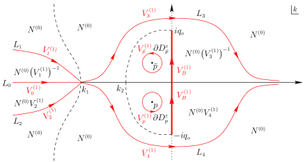
         Figure 6.10. Plane wave in the transmission/wake regime ($p\in D_{3}$) for $v_{s}<\xi<v_{o}$: the fourth and final stage of the first deformation. The jump contours $L_{3}$ and $L_{4}$ have been lifted away from the branch points $\pm iq_{o}$ similarly to [BM2].

         Third deformation (Figure 6.11). This deformation is different than the one of Figure 4.6 in that the disks $\overline{D_{p}^{\varepsilon}}$ and $\overline{D_{\bar{p}}^{\varepsilon}}$ now lie between the contours $L_{4}$ and $L_{3}$ and hence inside these disks we have $N^{(3)}=N^{(2)}$. Thus, the jumps (4.75hvkap) now remain invariant while the remaining jumps of problem (4.75hvkao) are modified as in the second deformation (4.17) but with $d^{\frac{1}{2}}$ now holding the role of $\delta$. Eventually, we find that $N^{(3)}$ satisfies the same problem as in Subsection 4.1.

         

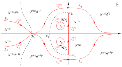
         Figure 6.11. Plane wave in the transmission/wake regime ($p\in D_{3}$) for $v_{s}<\xi<v_{o}$: the third deformation.

         Fourth deformation. This is identical to (4.46), leading to Riemann-Hilbert problem (4.50).

         In summary, in the range $v_{s}<\xi<v_{o}$ the original Riemann-Hilbert problem (3.16) can be deformed to Riemann-Hilbert problem (4.50) both for $p\in D_{1}$ and for $p\in D_{3}$. Thus, performing the analysis of Subsection 4.3, we obtain once again the phase-shifted plane wave (2.18).

         For $v_{o}<\xi<0$, the phase function changes from $\theta$ to $h$. Recall that for $p\in D_{1}$ the asymptotics is given by the phase-shifted modulated elliptic wave (2.19) throughout the range $(v_{o},0)$. Now, however, $p\in D_{3}$ and hence, as noted in the relevant discussion of Subsection 4.4, there is a value $v_{w}\in(v_{o},0)$ for which the contour $\widetilde{B}$ crosses the pole $p$ en route to collapsing onto $B$. Indeed, this value is the unique solution of equation (4.75gp) in the interval $(v_{o},0)$. Thus, similarly to the case $p\in D_{2}^{-}$, a soliton wake arises from the dominant component of Riemann-Hilbert problem (4.75hn) at $\xi=v_{w}$. In fact, the dominant problem is precisely that of Subsection 6.1. Therefore, at $\xi=v_{w}$ the leading-order asymptotics is characterized by (2.25) as the soliton wake (2.26) on top of the modulated elliptic wave $q_{\text{mew},w}(t)$. Finally, for $v_{o}<\xi<v_{w}$ and $v_{w}<\xi<0$ the jumps along $\partial D_{p}^{\varepsilon}$ and $\partial D_{\bar{p}}^{\varepsilon}$ are not part of the dominant problem and, like in the transmission regime, the leading-order asymptotics is given by the phase-shifted modulated elliptic wave (2.19). We note that, like in the trap/wake regime (see Remark 6.1), the soliton at $v_{s}$ induces a phase shift of $4\arg\left[p+\lambda(p)\right]$ in the asymptotics but no phase shift is generated by the soliton wake at $v_{w}$.

         The proof of Theorem 2.4 for the leading-order asymptotics in the transmission/wake regime $p\in D_{3}$ is complete.

         7. Conclusions

         In summary, we have characterized the interactions between solitons and localized disturbances in focusing media governed by the NLS equation. We reiterate that the main points of novelty of the results are on one hand the existence of a trapping regime, in which the velocity of the soliton differs from that of the case without radiation, and on the other hand the existence of mixed transmission/wake and trap/wake regimes, in which a single discrete eigenvalue gives rise to $O(1)$ contributions at two different velocities in the long-time asymptotics.

         The applicability of the deformations used in the present work requires that one can extend the reflection coefficient into the complex plane. As in [BM2], this can be done as long as the potential decays to background sufficiently rapidly (according to (1.3)) so as to ensure the existence of a Bargmann strip of analyticity.

         Regarding the wake formulae, we note that the expression for the solution at the wake coincides formally with that of a soliton on top of an elliptic background. On the other hand, crossing the wake does not result in an additional phase shift for the solution, while crossing a soliton does (cf. Remark 2.3). We also emphasize that the asymptotic expressions for the solution are not uniform with respect to $\xi$, as one can see by taking the limit of the various expressions as $\xi\to v_{s}$, $\xi\to\widetilde{v}_{s}$ and $\xi\to v_{w}$.

         We should mention that there exists previous literature on the interaction of solitons and the radiation on a nonzero background for integrable systems by the Riemann-Hilbert approach. See, for example, [KT] for the case of the Toda lattice and [AELT] for the case of the KdV equation. To the best of our knowledge, however, none of the previous cases studied in the literature give rise to the phenomena presented here, in which a localized disturbance results in a change of the soliton velocity and/or the production of a wake.

         We believe that the asymptotic formulae giving rise to a soliton on top of an elliptic wave should be a limiting reduction of 3-phase solutions of the focusing NLS equation. In this regard, we should mention that, in [BBEIM], the authors consider elliptic solutions of the focusing NLS equation as well as solutions corresponding to a nonlinear superposition of a soliton and hyperelliptic solutions. (We also note that reductions of 2-phase solutions of the focusing NLS equations, which give rise to solitons on a constant background, were studied in [BG].) The authors of [BBEIM] show that, in the genus-1 reduction, their solution reduces to the cnoidal wave solution of focusing NLS, namely (4.5.1) in [BBEIM]. Importantly, however, the dn solution is not the most general periodic solution of the focusing NLS equation (e.g., see [K1, K2, DS]). More precisely, the dn solution is just one of the special cases corresponding to a trivial phase. It is also the case that the modulate elliptic waves arising in the long-time asymptotics are not simply dn solutions. Therefore, it is doubtful that the formulae for the soliton on top of an elliptic wave in our work reduce to those in [BBEIM].

         The asymptotic expressions in our work remain valid in the limit $\xi\to 0$. As shown in [BLM1], in this limit $m\to 1$ and the solution reduces to the well-known sech-shaped soliton solution of the focusing NLS equation. However, some details of the derivation are different in this case and hence we omit the details for brevity. It is also the case that the asymptotic formulae remain valid in the limit $p_{\textnormal{re}}\to 0$, i.e. when the discrete eigenvalue lies on the imaginary axis. In this case, the velocity $v_{s}$ is zero (cf. (2.10)). Thus, one does not see the soliton in the plane wave region. Moreover, when $\xi=0$, the points $\alpha$, $\bar{\alpha}$ and $k_{o}$ in the definition (2.5) of $h$ collapse to $iq_{o}$, $-iq_{o}$ and $0$, respectively, and hence $h(0,k)=-2\left(k^{2}+q_{o}^{2}\right)$. Thus, for $p_{\textnormal{re}}=0$ we have $\text{Im}(h)(0,p)=0$, i.e. for $p_{\textnormal{re}}=0$ the imaginary parts of both $\theta$ and $h$ are zero at $\xi=0$. Therefore, in this case the velocity $\widetilde{v}_{s}$ of the trapped soliton coincides with the unperturbed velocity $v_{s}$.

         Another interesting special case is that of a pole $p$ lying on the branch cut $i[-q_{o},q_{o}]$, which gives rise to an Akhmediev breather. There are four different considerations: (i) Akhmediev breathers are periodic in $x$, and are therefore outside the class of initial conditions for which the inverse scattering transform formalism of [BK, BM2] applies (namely, constant nonzero boundary conditions); (ii) Neglecting the direct problem in the inverse scattering transform, one could still consider the Riemann-Hilbert problem with a pole in the branch cut and ask what happens then. Nonetheless, even the simple formulation of a Riemann-Hilbert problem with a pole in the branch cut requires some care; (iii) Akhmediev breathers are homoclinic in $t$ (i.e. they decay to the background as $t\to\pm\infty$) and hence they do not appear in the long-time asymptotics. However, one can still see the result of their presence in the phase difference of the background before/after the breather; (iv) Indeed, one can look at the case of a pole $p$ on the branch cut as a limit of the case of $p\in D_{3}$. Therefore, the case of an Akhmediev breather can be viewed as a limit of the trap/wake scenario. Then, the analysis shows that one will see a wake located at $\xi=0$ (for the same reasons as those outlined in the previous paragraphs).

         As usual, the inverse scattering transform is formulated under the assumption of existence and uniqueness of solutions. The well-posedness of IVP (1.1) for short times with initial conditions in suitable Sobolev spaces was recently proved in [Mu]. The question of global well-posedness for initial conditions in the space (1.3) is still open. In general, the issue of existence and uniqueness of solutions of the Riemann-Hilbert problems associated with the inverse scattering transform for integrable nonlinear partial differential equations is a nontrivial one [BDT, Z, TO]. Therefore, since this issue is peripheral to the main thrust of this work, we do not consider it here. However, we note that the asymptotic results provide an explicit solution of the Riemann-Hilbert problem (and hence of the IVP) modulo the solution of the error Riemann-Hilbert problem, which is a small-norm problem and, therefore, is expected to have a unique solution. On the other hand, whether the corresponding solution of the NLS equation belongs to the same function space (1.3) remains an interesting open question. We note that proving well-posedness of an IVP in a given function space through the inverse scattering transform is in general a nontrivial problem.

         Acknowledgements. We would like to thank M. Ablowitz, G. El and P. Miller for many insightful discussions. This work was partially supported by the National Science Foundation under grant number DMS-1614623. Finally, we are indebted to the anonymous referees whose constructive criticism led to the improvement of our paper.

         A. Appendix: Soliton Solutions

         The pure one-soliton solution of the focusing NLS IVP (1.5) can be derived by solving Riemann-Hilbert problem (3.7) together with the residue conditions (3.12) in the case of a zero reflection coefficient, i.e. by solving the problem

         $$M^{+}(x,t,k)=M^{-}(x,t,k)V_{1,0}(k), k\in\mathbb{R},$$ (4.75hvkaa)

         $$M^{+}(x,t,k)=M^{-}(x,t,k)V_{2,0}(k), k\in B^{+},$$ (4.75hvkab)

         $$M^{+}(x,t,k)=M^{-}(x,t,k)V_{3,0}(k), k\in B^{-},$$ (4.75hvkac)

         $$M(x,t,k)=I+O\left(\tfrac{1}{k}\right),\quad k\to\infty,$$ (4.75hvkad)

         $$\underset{k=p}{\text{Res}}\,M(x,t,k)=\left(0,c_{p}\,e^{2i\vartheta(x,t,p)}M_{1}(x,t,p)\right), x,t\in\mathbb{R},$$ (4.75hvkae)

         $$\underset{k=\bar{p}}{\text{Res}}\,M(x,t,k)=\left(c_{\bar{p}}\,e^{-2i\vartheta(x,t,\bar{p})}M_{2}(x,t,\bar{p}),0\right),\quad x,t\in\mathbb{R},$$ (4.75hvkaf)

         where the relevant jump matrices are given by

         $$V_{1,0}(k)=\begin{pmatrix}\dfrac{1}{d(k)}&0\\ 0&d(k)\end{pmatrix},\ \ V_{2,0}(k)=\begin{pmatrix}0&\dfrac{2\lambda(k)}{i\bar{q}_{-}}\\ \dfrac{\bar{q}_{-}}{2i\lambda(k)}&0\end{pmatrix},\ \ V_{3,0}(k)=\begin{pmatrix}0&\dfrac{q_{-}}{2i\lambda(k)}\\ \dfrac{2\lambda(k)}{iq_{-}}&0\end{pmatrix}$$ (4.75hvkb)

         with the functions $\lambda$ and $d$ defined by (2.2) and (3.4), and where the phase function $\vartheta$ is defined as

         $$\vartheta(x,t,k):=\lambda(k)\left(x-2kt\right)$$ (4.75hvkc)

         with $M_{1}$ and $M_{2}$ denoting the first and second column of $M$ respectively.

         The jump $V_{1,0}$ of problem (4.75hvka) along $\mathbb{R}$ can be eliminated via the transformation

         $$M^{(1)}=\left\{\begin{array}[]{ll}M\left(\begin{array}[]{cc}d^{\frac{1}{2}}&0\\ 0&d^{-\frac{1}{2}}\end{array}\right)&k\in\mathbb{C}^{+}\setminus B^{+},\\ M\left(\begin{array}[]{cc}d^{-\frac{1}{2}}&0\\ 0&d^{\frac{1}{2}}\end{array}\right)&k\in\mathbb{C}^{-}\setminus B^{-},\end{array}\right.$$ (4.75hvkd)

         which implies the following Riemann-Hilbert problem for $M^{(1)}$:

         $$M^{(1)+}=M^{(1)-}V_{B}, k\in B,$$ (4.75hvkea)

         $$M^{(1)}=I+O\left(\tfrac{1}{k}\right),\quad k\to\infty,$$ (4.75hvkeb)

         $$\underset{k=p}{\text{Res}}\,M^{(1)}(x,t,k)=\left(0,\varrho_{p}(x,t)M_{1}^{(1)}(x,t,p)\right), x,t\in\mathbb{R},$$ (4.75hvkec)

         $$\underset{k=\bar{p}}{\text{Res}}\,M^{(1)}(x,t,k)=\left(-\overline{\varrho_{p}(x,t)}M_{2}^{(1)}(x,t,\bar{p}),0\right),\quad x,t\in\mathbb{R},$$ (4.75hvked)

         where the jump matrix $V_{B}$ is defined in (4.8) and, recalling the definitions (3.11) and the symmetry (4.75ce), we have introduced the quantity

         $$\varrho_{p}(x,t):=\frac{C_{p}}{a^{\prime}(p)}e^{2i\vartheta(x,t,p)}.$$ (4.75hvkf)

         Problem (4.75hvke) can be solved by using the factorization

         $$M^{(1)}=M^{(2)}W,$$ (4.75hvkg)

         where $W$ is the solution of the continuous spectrum component of problem (4.75hvke), i.e.

         $$W^{+} =W^{-}V_{B}, k\in B,$$ (4.75hvkha)

         $$W =I+O\left(\tfrac{1}{k}\right),\quad k\to\infty,$$ (4.75hvkhb)

         and, similarly to problem (4.75ch), is given by the explicit formula

         $$W=\frac{1}{2}\begin{pmatrix}\Lambda(k)+\Lambda^{-1}(k)&-\frac{q_{o}}{\bar{q}_{-}}\left[\Lambda(k)-\Lambda^{-1}(k)\right]\\ -\frac{q_{o}}{q_{-}}\left[\Lambda(k)-\Lambda^{-1}(k)\right]&\Lambda(k)+\Lambda^{-1}(k)\end{pmatrix}$$ (4.75hvki)

         with $\Lambda(k)$ defined by (4.70).

         In turn, $M^{(2)}$ is the solution of the discrete spectrum component of problem (4.75hvke), i.e. $M^{(2)}$ is analytic for all $k\in\mathbb{C}$ apart from the poles $p$ and $\bar{p}$, where it satisfies the residue conditions

         $$\underset{k=p}{\text{Res}}\,M_{1}^{(2)}=-W_{21}(p)c_{p}\,d(p)M_{1}^{(1)}(p),\quad \underset{k=p}{\text{Res}}\,M_{2}^{(2)}=W_{11}(p)c_{p}\,d(p)M_{1}^{(1)}(p),$$ (4.75hvkja)

         $$\underset{k=\bar{p}}{\text{Res}}\,M_{1}^{(2)}=W_{22}(\bar{p})c_{\bar{p}}\,d(\bar{p})M_{2}^{(1)}(\bar{p}), \underset{k=\bar{p}}{\text{Res}}\,M_{2}^{(2)}=-W_{12}(\bar{p})c_{\bar{p}}\,d(\bar{p})M_{2}^{(1)}(\bar{p}).$$ (4.75hvkjb)

         Furthermore, $M^{(2)}$ satisfies the asymptotic condition

         $$M^{(2)}=I+O\left(\frac{1}{k}\right),\quad k\to\infty.$$ (4.75hvkk)

         Therefore, similarly to Subsection 4.2, we infer that $M^{(2)}$ is of the form

         $$M^{(2)}=I+\frac{\underset{k=p}{\text{Res}}\,M^{(2)}}{k-p}+\frac{\underset{k=\bar{p}}{\text{Res}}\,M^{(2)}}{k-\bar{p}}.$$ (4.75hvkl)

         Expressions (4.75hvkg), (4.75hvki), (4.75hvkj) and (4.75hvkl) yield

         $$M^{\textnormal{dom}}_{1}(p)=\frac{-\mathcal{B}\overline{\varrho_{p}}W_{2}(\bar{p})+\left(1+\overline{\mathcal{A}\varrho_{p}}\right)W_{1}(p)}{\left(1+\overline{\mathcal{A}\varrho_{p}}\right)\left(1+\mathcal{A}\varrho_{p}\right)-\mathcal{B}^{2}|\varrho_{p}|^{2}},$$ (4.75hvkma)

         $$M^{\textnormal{dom}}_{2}(\bar{p})=\frac{\left(1+\mathcal{A}\varrho_{p}\right)W_{2}(\bar{p})-\mathcal{B}\varrho_{p}W_{1}(p)}{\left(1+\overline{\mathcal{A}\varrho_{p}}\right)\left(1+\mathcal{A}\varrho_{p}\right)-\mathcal{B}^{2}|\varrho_{p}|^{2}}$$ (4.75hvkmb)

         with the constants $\mathcal{A}$, $\mathcal{B}$ given by (4.75cs). Hence, in view of (4.75hvkl) and (4.75hvkj), the function $M^{(2)}$ has been determined.

         Then, reverting the transformations (4.75hvkg) and (4.75hvkd) we obtain the solution $M$ of problem (4.75hvka) which, combined with the reconstruction formula (3.13), yields the pure one-soliton solution of IVP (1.5) for the focusing NLS equation in the form

         $$q(x,t) =q_{-}-\frac{i}{2}\left\{\left[1+\overline{\mathcal{A}\varrho_{p}(x,t)}\right]\left[1+\mathcal{A}\varrho_{p}(x,t)\right]-\mathcal{B}^{2}\left|\varrho_{p}(x,t)\right|^{2}\right\}^{-1}$$

         $$\ \cdot\bigg{\{}\!\left[1+\overline{\mathcal{A}\varrho_{p}(x,t)}\right]\varrho_{p}(x,t)\left[\Lambda(p)+\Lambda^{-1}(p)\right]^{2}+\left[1+\mathcal{A}\varrho_{p}(x,t)\right]\overline{\varrho_{p}}(x,t)\,\frac{q_{-}}{\bar{q}_{-}}\left[\overline{\Lambda(p)-\Lambda^{-1}(p)}\right]^{2}$$

         $$\hskip 28.45274pt-2\mathcal{B}\left|\varrho_{p}(x,t)\right|^{2}\,\frac{q_{o}}{\bar{q}_{-}}\left[\Lambda(p)+\Lambda^{-1}(p)\right]\left[\overline{\Lambda(p)-\Lambda^{-1}(p)}\right]\bigg{\}}.$$ (4.75hvkn)

         Actually, letting

         $$\chi(x,t):=-2\text{Im}\big{[}\vartheta(x,t,p)\big{]}+\ln\left|\frac{C_{p}}{a^{\prime}(p)}\right|,\quad\psi(x,t):=2\text{Re}\big{[}\vartheta(x,t,p)\big{]}+\arg\left(\frac{C_{p}}{a^{\prime}(p)}\right)$$ (4.75hvko)

         allows us to express the quantity $\varrho_{p}$ defined by (4.75hvkf) as

         $$\varrho_{p}(x,t)=e^{\chi(x,t)+i\psi(x,t)}.$$ (4.75hvkp)

         In turn, formula (A) takes the more compact form

         $$q(x,t)=q_{-}+\frac{e^{\chi(x,t)}\left(\bar{\mathcal{A}}\Lambda_{1}^{2}\bar{q}_{-}+\mathcal{A}\Lambda_{2}^{2}q_{-}-2\mathcal{B}\Lambda_{1}\Lambda_{2}q_{o}\right)+e^{i\psi(x,t)}\Lambda_{1}^{2}\bar{q}_{-}+e^{-i\psi(x,t)}\Lambda_{2}^{2}q_{-}}{4i\bar{q}_{-}\left[\sqrt{|\mathcal{A}|^{2}-\mathcal{B}^{2}}\cosh\!\big{(}\chi(x,t)+\ln\sqrt{|\mathcal{A}|^{2}-\mathcal{B}^{2}}\,\big{)}+\text{Re}\left(\mathcal{A}e^{i\psi(x,t)}\right)\right]}$$ (4.75hvkq)

         with the constants $\Lambda_{1}$ and $\Lambda_{2}$ given by (4.75da). It now becomes evident that the pure one-soliton is localized along the line $\chi(x,t)+\ln\sqrt{|\mathcal{A}|^{2}-\mathcal{B}^{2}}=0$ which in view of (4.75hvko) is equivalent to

         $$\text{Im}\big{[}\vartheta(x,t,p)\big{]}=\frac{1}{2}\left(\ln\left|\frac{C_{p}}{a^{\prime}(p)}\right|+\ \ln\sqrt{|\mathcal{A}|^{2}-\mathcal{B}^{2}}\right).$$ (4.75hvkr)

         Expressing the pure one-soliton in the non-standard form (4.75hvkq) allows us to compare it against the leading-order asymptotics (2.16), since both expressions involve two portions: the background (first term) and a traveling wave part (second term). To perform this comparison, we calculate the long-time asymptotics of (4.75hvkq). The pure one-soliton propagates along the line specified by equation (4.75hvkr). Noting that $\vartheta(x,t,k)=\theta(\xi,k)t$ (cf. definitions (4.75hvkc) and (2.3)), we infer that a necessary condition for equation (4.75hvkr) to hold in the limit $t\to\infty$ is that $\mathop{\rm Im}[\theta(\xi,p)]=0$. This last equation, however, amounts to $\xi=v_{s}$ (recall (2.10)-(2.11)). Thus, we consider three cases: $\xi<v_{s}$ (left of soliton); $\xi>v_{s}$ (right of soliton); $\xi=v_{s}$.

         If $\xi<v_{s}$ then $\mathop{\rm Im}[\theta(\xi,p)]>0$ (recall Figure 3.2). Hence, as $t\to\infty$ we have $\chi(x,t)\to-\infty$ and, in turn, $e^{\chi(x,t)}\to 0$ and $\cosh\!\big{(}\chi(x,t)+\ln\sqrt{|\mathcal{A}|^{2}-\mathcal{B}^{2}}\,\big{)}\to\infty$. Therefore, for $\xi<v_{s}$ we obtain

         $$q(x,t)=q_{-}+o(1),\quad t\to\infty,$$ (4.75hvks)

         in agreement with the asymptotics (2.14) apart from the real constant phase $g_{\infty}(\xi)$, which originates from the radiation of Riemann-Hilbert problem (3.7), (3.12) and which vanishes once the reflection coefficient in this problem is set to zero.

         If $\xi>v_{s}$ then $\mathop{\rm Im}[\theta(\xi,p)]<0$. Hence, as $t\to\infty$ we have $\chi(x,t)\to\infty$ and, therefore, $e^{\chi(x,t)}\to\infty$ and $\cosh\!\big{(}\chi(x,t)+\ln\sqrt{|\mathcal{A}|^{2}-\mathcal{B}^{2}}\,\big{)}\to\infty$. Thus, expressing $\cosh$ in exponential form we obtain

         $$q(x,t)=q_{-}+\frac{\bar{\mathcal{A}}\Lambda_{1}^{2}\bar{q}_{-}+\mathcal{A}\Lambda_{2}^{2}q_{-}-2\mathcal{B}\Lambda_{1}\Lambda_{2}q_{o}}{2i\bar{q}_{-}\left(|\mathcal{A}|^{2}-\mathcal{B}^{2}\right)}+o(1),\quad t\to\infty.$$ (4.75hvkt)

         Through algebraic manipulations, it can be shown that the leading-order term of (4.75hvkt) is equal to $q_{+}$, which is consistent with the fact that propagation along speeds $\xi>v_{s}$ always remains to the right of the soliton at $\xi=v_{s}$.

         Finally, if $\xi=v_{s}$ then $\mathop{\rm Im}[\theta(\xi,p)]=0$ and hence $\mathop{\rm Im}[\vartheta(x,t,p)]=0$, which implies

         $$\chi(v_{s}t,t)=\ln\left|\mathcal{R}_{p}\right|,\quad\psi(v_{s}t,t)=2\theta(v_{s},p)t+\arg\left(\mathcal{R}_{p}\right),\quad\mathcal{R}_{p}:=\frac{C_{p}}{a^{\prime}(p)}.$$

         Then, (4.75hvkq) becomes

         $$q(v_{s}t,t)$$ (4.75hvku)

         $$=q_{-}+\frac{\left|\mathcal{R}_{p}\right|\left(\bar{\mathcal{A}}\Lambda_{1}^{2}\bar{q}_{-}+\mathcal{A}\Lambda_{2}^{2}q_{-}-2\mathcal{B}\Lambda_{1}\Lambda_{2}q_{o}\right)+e^{i\left[2\theta(v_{s},p)t+\arg(\mathcal{R}_{p})\right]}\Lambda_{1}^{2}\bar{q}_{-}+e^{-i\left[2\theta(v_{s},p)t+\arg(\mathcal{R}_{p})\right]}\Lambda_{2}^{2}q_{-}}{4i\bar{q}_{-}\left\{\sqrt{|\mathcal{A}|^{2}-\mathcal{B}^{2}}\cosh\big{[}\ln\big{(}|\mathcal{R}_{p}|\sqrt{|\mathcal{A}|^{2}-\mathcal{B}^{2}}\,\big{)}\big{]}+\mathop{\rm Re}\big{(}\mathcal{A}e^{i\left[2\theta(v_{s},p)t+\arg(\mathcal{R}_{p})\right]}\big{)}\right\}}.$$

         The exact one-soliton solution (4.75hvku) is the same with the leading-order asymptotics (2.16) except for three points: (i) the background, which is $q_{-}$ in (4.75hvku) and $q_{-}e^{2ig_{\infty}(v_{s})}$ in (2.16); (ii) an overall phase of $e^{2ig_{\infty}(v_{s})}$, which is present in (2.16) but not in (4.75hvku); (iii) the quantity $\mathcal{R}_{p}$ in (4.75hvku), which is replaced by $R_{p}$ in (2.16), where $R_{p}=\mathcal{R}_{p}\delta^{2}(v_{s},p)e^{-2ig(v_{s},p)}$. However, this variation is exclusively due to the presence of radiation in IVP (1.5). Indeed, setting the reflection coefficient equal to zero in the definitions (4.19), (4.49) and (4.66) of $\delta$, $g$ and $g_{\infty}$ yields $\delta(v_{s},p)=g(v_{s},p)=g_{\infty}(v_{s})=0$, i.e. in the absence of radiation (2.16) would be identical to (4.75hvku).

         Gino Biondini                              Sitai Li                                        Dionyssios Mantzavinos
         Department of Mathematics         Department of Mathematics Department of Mathematics
         State University of New York        University of Michigan                  University of Kansas
         Buffalo, NY 14260                       Ann Arbor, MI 48109                    Lawrence, KS 66045
         E-mail: biondini@buffalo.edu         E-mail: sitaili@umich.edu               E-mail: mantzavinos@ku.edu

References

- [AS] M. Ablowitz and H. Segur, Solitons and the inverse scattering transform, SIAM, 1981.
- [AK] N. Akhmediev and V. Korneev, Modulational instability and periodic solutions of the nonlinear Schrödinger equation. Theor. Math. Phys. 69 (1987), 1089-1093.
- [AELT] K. Andreiev, I. Egorova, T. Lange and G. Teschl, Rarefaction waves of the Korteweg-de Vries equation via nonlinear steepest descent. J. Differential Equations 261 (2016), 5371-5410.
- [BDT] R. Beals, P. Deift and C. Tomei, Direct and inverse scattering on the line, American Mathematical Society, 1988.
- [BBEIM] E. Belokolos, A. Bobenko, V. Enol’ski, A. Its and V. Matveev, Algebro-geometric approach to nonlinear integrable equations, Springer-Verlag, 1994.
- [BF] T. Benjamin and J. Feir, The disintegration of wave trains on deep water. J. Fluid Mech. 27 (1967).
- [BG] M. Bertola and P. Giavedoni, A degeneration of two-phase solutions of the focusing nonlinear Schrödinger equation via Riemann-Hilbert problems. J. Math. Phys. 56 (2015), 061507.
- [BMi] D. Bilman and P. Miller, A robust inverse scattering transform for the focusing nonlinear Schrödinger equation. arXiv:1710.06568, to appear in Comm. Pure Appl. Math.
- [BF] G. Biondini and E. Fagerstrom, The integrable nature of modulational instability. SIAM J. Appl. Math. 75 (2015), 136-163.
- [BK] G. Biondini and G. Kovačič, Inverse scattering transform for the focusing nonlinear Schrödinger equation with nonzero boundary conditions. J. Math. Phys. 55 (2014), 031506.
- [BLM1] G. Biondini, S. Li and D. Mantzavinos, Oscillation structure of localized perturbations in modulationally unstable media. Phys. Rev. E 94 (2016), 060201(R).
- [BLM2] G. Biondini, S. Li and D. Mantzavinos, Soliton trapping, transmission and wake in modulationally unstable media. Phys. Rev. E 98 (2018), 042211.
- [BLMT] G. Biondini, S. Li, D. Mantzavinos and S. Trillo, Universal behavior of modulationally unstable media. SIAM Review 60 (2018), 888-908.
- [BM1] G. Biondini and D. Mantzavinos, Universal nature of the nonlinear stage of modulational instability. Phys. Rev. Lett. 116 (2016), 043902.
- [BM2] G. Biondini and D. Mantzavinos, Long-time asymptotics for the focusing nonlinear Schrödinger equation with nonzero boundary conditions at infinity and asymptotic stage of modulational instability. Comm. Pure Appl. Math. 70 (2017), 2300-2365.
- [BKS] A. Boutet de Monvel, V. Kotlyarov and D. Shepelsky, Focusing NLS equation: Long-time dynamics of step-like initial data. Int. Math. Res. Not. 2011 (2011), 1613-1653.
- [BV] R. Buckingham and S. Venakides, Long-time asymptotics of the nonlinear Schrödinger equation shock problem. Comm. Pure Appl. Math. 60 (2007), 1349-1414.
- [DS] B. Deconinck and B. Segal, The stability spectrum for elliptic solutions to the focusing NLS equation. Phys. D 346 (2017), 1-19.
- [DKKZ] P. Deift, S. Kamvissis, T. Kriecherbauer and X. Zhou, The Toda rarefaction problem. Comm. Pure Appl. Math. 49 (1996), 35-83.
- [DZ1] P. Deift and X. Zhou, A steepest descent method for oscillatory Riemann-Hilbert problems. Asymptotics for the mKdV equation. Ann. of Math. 137 (1993), 295-370.
- [DZ2] P. Deift and X. Zhou, Long-time behavior of the non-focusing nonlinear Schrödinger equation – a case study. New Series, Lectures in Mathematical Sciences 5, University of Tokyo, 1995.
- [DVZ1] P. Deift, S. Venakides and X. Zhou, The collisionless shock region for the long-time behavior of solutions of the KdV equation. Comm. Pure Appl. Math. 47 (1994), 199-206.
- [DVZ2] P. Deift, S. Venakides and X. Zhou, An extension of the steepest descent method for Riemann-Hilbert problems: the small dispersion limit of the Korteweg-de Vries (KdV) equation. Proc. Natl. Acad. Sci. USA 95 (1998), 450-454.
- [DPVV] F. Demontis, B. Prinari, C. van der Mee and F. Vitale, The inverse scattering transform for the focusing nonlinear Schrödinger equation with asymmetric boundary conditions. J. Math. Phys. 55 (2014), 101505.
- [EGKK] G. El, A. Gurevich, V. Khodorovskii and A. Krylov, Modulational instability and formation of a nonlinear oscillatory structure in a focusing medium, Phys. Lett. A 177 (1993), 357-361.
- [FL] M. Forest and J.-E. Lee, Geometry and modulation theory for periodic nonlinear Schrödinger equation, in Oscillation theory, computation and methods of compensated compactness, IMA Vol. Math. Appl. 2, C. Dafermos, J. Ericksen, D. Kinderlehrer, and M. Slemrod, Eds., Springer, New York, 1986.
- [GZ] A. Gelash and V. Zakharov, Superregular solitonic solutions: a novel scenario for the nonlinear stage of modulation instability. Nonlinearity 27 (2014), R1-R39.
- [JM] R. Jenkins and K.D.T.-R. McLaughlin, Semiclassical limit of focusing NLS for a family of square barrier initial data. Comm. Pure Appl. Math. 67 (2013), 246-320.
- [K1] A. Kamchatnov, Nonlinear periodic waves and their modulations, World Scientific, 2000.
- [K2] A. Kamchatnov, On improving the effectiveness of periodic solutions of the NLS and DNLS equations. J. Phys. A 23 (1990), 2945-2960.
- [KMM] S. Kamvissis, K.D.T.-R. McLaughlin and P. Miller, Semiclassical soliton ensembles for the focusing nonlinear Schrödinger equation, Princeton University Press, 2003.
- [KSER] A. Kraych, P. Suret, G. El and S. Randoux, Nonlinear evolution of the locally induced modulational instability in fiber optics. Phys. Rev. Lett. 122 (2019), 054101.
- [KT] H. Kruger and G. Teschl, Stability of the periodic Toda lattice in the soliton region. Int. Math. Res. Not. 2009 (2009), 3996-4031.
- [Ma] Y.-C. Ma, The perturbed plane-wave solutions of the cubic Schrödinger equation. Stud. Appl. Math. 60 (1979), 43-58.
- [Mi] P. Miller, Riemann-Hilbert problems with lots of discrete spectrum. Contemp. Math. 458 (2008), 163-181.
- [Mu] C. Muñoz, Instability in nonlinear Schrödinger breathers. Proyecciones J. Math. 36 (2017), 653-683.
- [PV] B. Prinari and F. Vitale, Inverse scattering transform for the focusing nonlinear Schrödinger equation with one-sided nonzero boundary conditions, Contemp. Math. 652 (2015), 157-194.
- [SA1] H. Segur and M. Ablowitz, Asymptotic solutions and conservation laws for the nonlinear Schrödinger equation. I. J. Math. Phys. 17 (1976), 710-713.
- [SA2] H. Segur and M. Ablowitz, Asymptotic solutions and conservation laws for the nonlinear Schrödinger equation. II. J. Math. Phys. 17 (1976), 714-716.
- [TW] S. Trillo and S. Wabnitz, Dynamics of the nonlinear modulational instability in optical fibers. Opt. Lett. 16 (1991), 986-988.
- [TO] T. Trogdon and S. Olver, Riemann-Hilbert problems, their numerical solution, and the computation of nonlinear special functions, SIAM, 2016.
- [W] G. Whitham, Linear and nonlinear waves, Wiley, 1974.
- [ZM] V. Zakharov and S. Manakov, Asymptotic behavior of nonlinear waves systems integrated by the inverse scattering method. Sov. Phys. JETP 44 (1976), 106-112.
- [ZG] V. Zakharov and A. Gelash, Nonlinear stage of modulation instability. Phys. Rev. Lett. 111 (2013), 054101.
- [ZO] V. Zakharov and L. Ostrovsky, Modulational instability: The beginning. Phys. D 238 (2009), 540-548.
- [ZS] V. Zakharov and A. Shabat, Exact theory of two-dimensional self-focusing and one-dimensional self-modulation of waves in nonlinear media. Sov. Phys. JETP 34 (1972), 63-69.
- [Z] X. Zhou, The Riemann-Hilbert problem and inverse scattering. SIAM J. Math. Anal. 20 (1989), 966-986.