Maya: Falsifying Power Sidechannels with Dynamic Control

Abstract.

The security of computers is at risk because of information leaking through physical outputs such as power, temperature, or electromagnetic (EM) emissions. Attackers can use advanced signal measurement and analysis to recover sensitive data from these sidechannels.

To address this problem, this paper presents Maya, a simple and effective solution against power side-channels. The idea is to re-shape the power dissipated by an application in an application-transparent manner using control theory techniques – preventing attackers from learning any information. With control theory, a controller can reliably keep power close to a desired target value even when runtime conditions change unpredictably. Then, by changing these targets intelligently, power can be made to appear in any desired form, appearing to carry activity information which, in reality, is unrelated to the application. Maya can be implemented in privileged software or in simple hardware. In this paper, we implement Maya on two multiprocessor machines using Operating System (OS) threads, and show its effectiveness and ease of deployment.

1. Introduction

There is an urgent need to secure computer systems against the growing number of cyberattack surfaces. An important class of these attacks is that which utilizes the physical outputs of a system, such as its power, temperature or electromagnetic (EM) emissions. These outputs are correlated with system activity and can be exploited by attackers to recover sensitive information (Yan et al., 2015; Michalevsky et al., 2015; Lifshits et al., 2018; Kocher et al., 2011; Zhou and Feng, 2005).

Many computing systems ranging from mobile devices to multicore servers in the cloud are vulnerable to physical side channel attacks (Yan et al., 2015; Michalevsky et al., 2015; Lifshits et al., 2018; Zhang et al., 2016; Yang et al., 2017; Masti et al., 2015). With advanced signal measurement and analysis, attackers can identify many details like keystrokes, password lengths (Yan et al., 2015), personal data like location, browser and camera activity (Lifshits et al., 2018; Yang et al., 2017; Michalevsky et al., 2015), and the bits of encryption keys (Kocher et al., 2011).

Many defenses against physical sidechannels have been proposed which aim to keep the physical signals constant or noisy (Tiri and Verbauwhede, 2005; Saputra et al., 2003; Yang et al., 2005; Das et al., 2017; Kocher et al., 2011; Yang et al., 2012; Avirneni and Somani, 2014). However, all these techniques require new hardware and, hence, existing systems in the field are left vulnerable. Trusted execution environments like Intel SGX (McKeen et al., 2013) or ARM TrustZone (ARM, 2009) cannot “contain” physical signals and are ineffective to stop information leaking through them (Benhani and Bossuet, 2018; Bukasa et al., 2018; Masti et al., 2015).

To address this problem, we seek a solution that is simple to implement and is effective against power side-channels. The idea is to rely on privileged software or simple hardware to distort, in an application-transparent manner, the power dissipated by an application — so that the attacker cannot glean any information. Obfuscating power also removes leakage through temperature and EM signals, since they are directly related to the computer’s power (Callan et al., 2015; Bukasa et al., 2018; Masti et al., 2015). Such a defense can prevent exploits that analyze application behavior at the scale of several milliseconds or longer, such as those that infer what applications are running, what data is used in the camera or browser, or what keystrokes occur (Lifshits et al., 2018; Yan et al., 2015).

A first challenge in building an easily deployable power-shaping defense is the lack of configurable system inputs that can effectively change power. Dynamic Voltage and Frequency Scaling (DVFS) is an input supported by nearly all mainstream processors (Rotem et al., 2012; Rotem, 2015; Toprak-Deniz et al., 2014; Beck et al., 2018; ARM, [n. d.]b, [n. d.]a). However, DVFS levels are only a few, and the achievable range of power values depends on the application — compute-intensive phases have higher values of power and show bigger changes with DVFS, while it is the opposite for memory-bound applications. Injecting idle cycles in the system (van de Ven and Pan, [n. d.]; Lezcano, [n. d.]) is another technique, but it can only reduce power and not increase it.

The second and more important challenge is to develop an algorithm that reshapes power to effectively eliminate any information leakage. This is hard because applications vary widely in their activity profile and in how they respond to system inputs. Attempts to maintain constant power, insert noise into power signals, or simply randomize DVFS levels have been unsuccessful (Lifshits et al., 2018; Real et al., 2008; Zhang et al., 2016). These techniques only tend to add noise, but do not mask application activity (Real et al., 2008; Zhang et al., 2016).

In this work, we propose Maya, a defense architecture that intelligently re-shapes a computer’s power in an application-transparent manner, so that the attacker cannot extract application information. To achieve this, Maya uses a Multiple Input Multiple Output (MIMO) controller from control theory (Skogestad and Postlethwaite, 2005). This controller can reliably keep power close to a target power level even when runtime conditions change unpredictably. By changing these targets intelligently, power can be made to appear in any desired form, appearing to carry activity information which, in fact, is unrelated to the application.

Maya can be implemented in privileged software or in simple hardware. In this paper, we implement Maya on two multicore machines using OS threads. The contributions of this work are:

1. Maya, a new defense system against power side-channels through power re-shaping.

2. An implementation of Maya using only privileged software. To the best of our knowledge, this is the first software defense against power side-channels that is application-transparent.

3. The first application of MIMO control theory to side-channel defense.

4. An analysis of power-shaping properties necessary to mask information leakage.

5. An evaluation of Maya using machine learning-based attacks on two different real machines.

2. Background

2.1. Physical Side-Channels

Physical side-channels such as power, temperature, and electromagnetic (EM) emissions carry significant information about the execution. For example, these side channels have been used to infer the characters typed by a smartphone user (Lifshits et al., 2018), to identify the running application, login requests, and the length of passwords on a commodity smartphone (Yan et al., 2015), and even to recover the full encryption key from a cryptosystem (Kocher et al., 1999).

All power analysis attacks rely on the principle that the dynamic power of a computing system is directly proportional to the switching activity of the hardware. Since this activity varies across instructions, groups of instructions, and application tasks, they all leave distinct power traces (Vasilakis, 2015; Shao and Brooks, 2013; Lifshits et al., 2018; Yan et al., 2015). By analyzing these power traces, many details about the execution can be deduced. Temperature and EM emissions are also directly related to a computer’s power consumption and techniques to analyze them are similar (Callan et al., 2015; Bukasa et al., 2018; Masti et al., 2015).

Physical side-channels can be sensed through special measurement devices (Kocher et al., 2011), unprivileged hardware and OS counters (Rotem et al., 2012; and, [n. d.]), public amenities like USB charging stations (Yang et al., 2017), malicious smart batteries (Lifshits et al., 2018) or remote antennas that measure EM emissions (Genkin et al., 2016; Genkin et al., 2014). In cloud systems, an application can use the thermal coupling between cores to infer the temperature profile of a co-located application (Masti et al., 2015).

After measuring the signals, attackers search for patterns in the signal over time like phase behavior and peak locations, and its frequency spectrum after a Fourier transform. This can be done through Simple Power Analysis (SPA), which uses a single trace (Lifshits et al., 2018; Genkin et al., 2016; Yan et al., 2015), or Differential Power Analysis (DPA), which examines the statistical differences between thousands of traces (Kocher et al., 2011; Zhang et al., 2016).

The timescale over which the signals are analyzed is determined by the information that attackers seek. For cryptographic keys, it is necessary to record and analyze signals over a few microseconds or faster (Kocher et al., 2011). For higher-level information like the details of the running applications, keystrokes, browser data, and personal information, signals are analyzed over timescales of milliseconds or more (Yang et al., 2017; Lifshits et al., 2018; Yan et al., 2015). The latter are the timescales that this paper focuses on.

2.2. Control Theory Techniques

Using control theory (Skogestad and Postlethwaite, 2005), we can design a controller $K$ that manages a system $S$ (i.e., a computer) as shown in Figure 1. The system has outputs $y$ (e.g., the power consumed) and configurable inputs $u$ (e.g., the DVFS level). The outputs must be kept close to the output targets $r$. The controller reads the deviations of the outputs from their targets ($\Delta y=r-y$), and sets the inputs.

Figure 1. Control loop.

The controller is a state machine characterized by a state vector, $x(T)$, which evolves over time $T$. It advances its state to $x(T+1)$ and generates the system inputs $u(T)$ by reading the output deviations $\Delta y(T)$:

(1) $$\begin{aligned} x(T+1)&=A\times x(T)+B\times\Delta y(T)\\ u(T)&=C\times x(T)+D\times\Delta y(T)\end{aligned}\quad x(0)=0$$

where $A$, $B$, $C$, and $D$ are matrices that encode the controller. The most useful controllers are those that actuate on Multiple Inputs and sense Multiple Outputs (MIMO) at the same time.

Designers can specify multiple parameters in the control system (Skogestad and Postlethwaite, 2005). They include the maximum bounds on the deviations of the outputs from their targets, the differences from design conditions or unmodeled effects that the controller must be tolerant to (i.e., the uncertainty guardband), and the relative priority of changing the different inputs, if there is a choice (i.e., the input weights). With these parameters, controller design is automated (Gu et al., 2013).

3. Threat Model

We assume that attackers try to compromise the victim’s security through power measurements. They measure power using off-the-shelf sensors present in the victim machine like hardware counters or OS APIs (Rotem et al., 2012; and, [n. d.]). Such sensors are only reliable at the time granularity of several milliseconds. Attackers could use alternative measurement strategies at this timescale like malicious USB charging booths (Yang et al., 2017), compromised batteries (Lifshits et al., 2018), thermal measurements (Masti et al., 2015), or cheap power-meters when physical access is possible (Wei et al., 2019).

We exclude power analysis attacks that search for patterns at a fine time granularity with special hardware support such as oscilloscopes (Kocher et al., 1999) or antennas (Genkin et al., 2016; Genkin et al., 2014). While such attacks are powerful enough to attack cryptographic algorithms (Kocher et al., 2011), they are harder to mount and need more expensive equipment. Even with fine-grain measurement, information about events like keystrokes can be analyzed only at the millisecond timescale (Lifshits et al., 2018; Yan et al., 2015).

We assume that attackers can know the algorithm used by Maya to reshape the computer’s power. They can run the algorithm and see its impact on the time-domain and frequency-domain behavior of applications. Using these observations, they can develop machine learning models to adapt to the defense and try defeating it.

Finally, we assume that the hardware or privileged software that implements the control system to reshape the power trace is uncompromised. In a software implementation, the OS scheduler and DVFS interfaces are assumed to be uncompromised.

4. Falsifying Power Side-channels with Control

We propose that a computer system defend itself against power side-channel attacks by distorting its pattern of power consumption. Unfortunately, this is hard to perform successfully. Simple distortions like adding noise to power signals can be removed by attackers using signal processing techniques. This is especially the case if, as we assume in this paper, the attacker knows the general algorithm that the defense uses to distort the signal. Indeed, past approaches have been unable to provide a solution to this problem. In this paper, we propose a new approach. In the following, we describe the rationale behind the approach, present the high-level architecture, and discuss how to generate the distortion to falsify information leakage through power signals.

4.1. Why Use Control Theory Techniques?

To understand why control theory techniques are necessary at shaping power, consider the following scenario. We measure the power consumed by an application at fixed timesteps to record a trace, as shown in Figure 2a. To prevent information leakage, we must distort the power trace into a different uncorrelated shape.

Assume that the system has a mechanism to increase the power consumed, and another to reduce it. In this paper, these mechanisms are the ability to run a Balloon thread and an idle thread, respectively, for a chosen amount of time. A balloon thread is one that performs power-consuming operations (e.g., floating-point operations) in a tight loop, and an idle thread forces the processor into an idle state.

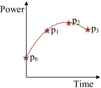
(a) Original

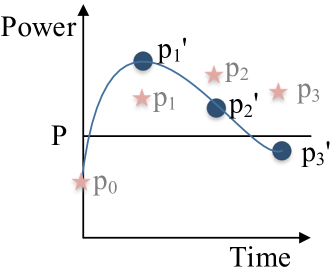
(b) Distorted

Figure 2. Example of the power trace for an application.

One way to mislead the attacker is to keep the power consumption at another level $P$ (Figure 2b). To achieve this, we can measure the difference between $P$ and the actual power $p_{i}$ at each timestep and schedule a balloon thread if $P-p_{i}>0$ or an idle thread otherwise. Unfortunately, this approach is too simplistic to be effective. First, it ignores how the application’s power changes intrinsically. Second, achieving the power $P$ with this application may require a combination of both the idle and balloon threads. When only a balloon thread is scheduled at the 0^th timestep based on $P-p_{0}$, the power in the 1^st timestep would be $p_{1}^{\prime}$ rather than our target $P$.

If this poor control algorithm is repeatedly applied, it will always miss the target and we obtain the trace in Figure 2b where the measured power is not close to the target, and in addition, has enough features of the original trace.

An approach with control theory is able to get much closer to the target power level. This is because the controller makes more informed power changes at every interval and can set multiple inputs for accurate control. To understand why, we rephrase the equations of controller operation (Equation 1) slightly:

(2) $$State(T+1) =A\times State(T)+B\times Error(T)$$

$$Action(T) =C\times State(T)+D\times Error(T)$$

The second equation shows that the action taken at time $T$ (in our case, scheduling the balloon and idle threads) is a function of the tracking error observed at time $T$ (in our case, $P$-$p_{0}$) and the controller’s state. The state is a summary of the controller’s experience in regulating the application. The new state used in the next timestep is determined by the current state and error serving as an “accumulated experience” to smoothly and quickly reach the target.

Further, the controller’s actions and state evolution are influenced by the matrices $A$, $B$, $C$, and $D$, which were generated when the controller was designed. This design includes running a training set of applications while scheduling the balloon and idle threads and measuring the resulting power changes. Consequently, these matrices embed the intrinsic behavior of the applications under these conditions.

Overall, with a control theory controller the measured power trace will be much closer to the target signal. If the target signal is chosen appropriately, the attacker can longer recover the application information.

4.2. High-Level Architecture

The high-level architecture of a system that uses control theory techniques to reshape the power trace of a computer system is shown in Figure 3. It is composed of a Mask Generator and a Controller. The Mask Generator decides what should the target power be at each time, so that it can mislead any attacker. It continuously communicates its target power to the controller. In the example of Section 4.1, the Mask Generator would pass the constant value $P$ to the controller. Section 4.3 discusses more advanced cases that involve passing a time-varying function.

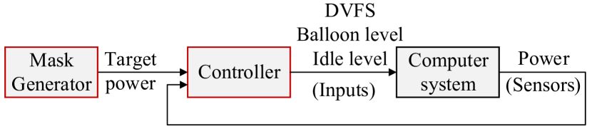
Figure 3. High-level architecture of a system that falsifies the power trace of an application.

The controller reads this target and the actual power consumed by the computer system, as given by power sensors. Then, based on its current state, it actuates on various inputs of the computer system, which will bring the power close to the target power. Some of the possible actuations are: changing the frequency and voltage of the computer system, and scheduling the balloon thread or the idle thread.

The space of power side-channel attack environments is broad, which calls for different architectures. Table 1 shows two representative environments, which we call Conventional and Specialized environments. The Conventional environment is one where the attacker extracts information through off-the-shelf sensors such as power counters or OS API (Yan et al., 2015). Such sensors are typically reliable only at coarse measurement granularities – e.g., every 20ms. Hence, we can use a typical matrix-based controller, like the one described in Section 2.2, which can respond in 5–10$\mu$s. Given these timescales, the controller can actuate on parameters such as frequency or voltage, or schedule balloon or idle threads. Such controllers can be used to hide what application is running, or what keystroke is being pressed.

Table 1. Two types of power side-channel environments.

Characteristic	Conventional	Specialized
Attacker’s sensing	Reads power sensors like counters	Uses devices like oscilloscopes
Sensing rate	$\approx$ 20ms	¡ 50ns
Controller type	Matrix-based controller, in hardware or privileged software	Table-based controller in hardware
Controller Response Time	5–10$\mu$s	$\approx$ 10ns
Example Actuations	Change frequency and voltage; schedule balloon and idle threads	Insert instructions and pipeline bubbles
Example Use Cases	Hide what application runs or what keystroke occurred	Hide features of a crypto algorithm

The Specialized environment is one where the attacker extracts information using specialized hardware devices, such as oscilloscopes. The frequency of samples can be in the tens of nanoseconds. In this case, the controller has to be very fast. Hence, it cannot use the matrix-based approach of Section 2.2. Instead, tt has to rely on a table of pre-computed values. Its operation involves a table look-up that determines what action to take. This controller is implemented in hardware and has a response time of no more than around 10ns.

A possible design involves actuating on a hardware module that immediately inserts compute instructions into the ROB or pipeline bubbles to mislead any attacker. With such a fast actuation, this type of defense can be used, for example, to hide the features of a cryptographic algorithm.

In the rest of the paper, we focus on the first type of environment only, as it is by far the easiest to mount and widely used.

(a)

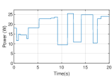
(b)

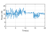
(c)

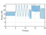
(d)

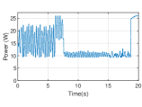
(e)

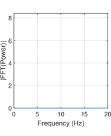
(a) Constant

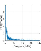
(b) Uniformly Random

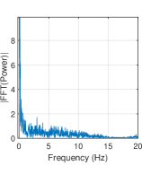
(c) Gaussian

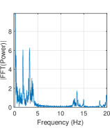
(d) Sinusoid

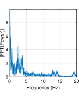
(e) Gaussian Sinusoid

Figure 4. Examples of different masks. In each case, the time-domain curve is at the top, and the frequency-domain one at the bottom.

4.3. Generating Effective Masks

To effectively mislead an attacker, it is not enough for the defense to only be able to track power targets closely (as discussed in Section 4.1). In addition, the defense must create an appropriate target power signal (i.e., an appropriate mask). The module that determines the mask to be used at each interval is the Mask Generator.

An effective mask must protect information leaked in both time domain and the frequency domain (i.e., after obtaining its FFT) because attackers can analyze signals in either domain.

We postulate that, to be effective, a mask must have three properties. First, its mean and variance must change over the time domain, to portray phase behavior (Figure 4(c) top). Such changes will mask the original signal in the time domain.

The second property is that the mean and variance changes must have various rates – from smooth to abrupt. This property will cause the resulting frequency domain curve to spread over a range of frequencies (Figure 4(c) bottom). As a result, the curve will a property similar to typical curves generated natively by applications.

The final property is that the target signal must have repeating patterns at various rates. This is to create various peaks in the frequency domain curve (Figure 4(e) bottom). Such peaks are common in applications, as they represent the effects of loops.

Table 2 lists some well-known signals, showing whether each signal changes the mean and the variance in the time domain, and whether it creates spread and peaks in the frequency domain. Such properties determine their viability to be used as effective masks. Figure 4 shows a graphical representation of each signal in order.

Table 2. Some standard signals and what they change in the time and frequency domains.

	Time-domain		Frequency-domain
Signal	Mean	Variance	Spread	Peaks
Constant	–	–	–	–
Uniformly Random	Yes	–	Yes	–
Gaussian	Yes	Yes	Yes	–
Sinusoid	Yes	Yes	–	Yes
Gaussian Sinusoid	Yes	Yes	Yes	Yes

A Constant signal (Figure 4(a)) does not change the mean or variance in the time domain, or create spread or peaks in the frequency domain. Note that this signal cannot be realized in practice. Any realistic method of keeping the output signal constant under changing conditions would have to first observe the outputs deviating from the targets, and then set the inputs accordingly. Hence, the output signal would have a burst of power activity at all the change points in the application. As a result, such signal would easily leak information. Furthermore, the signals obtained in multiple runs of a given application would be similar to each other.

In a Uniformly Random signal (Figure 4(b)), a value is chosen randomly from a range, and is used as a target for a random duration in the time domain. After this period, another value and duration are selected, and the process repeats. This signal changes the mean but not the variance in the time domain. In the frequency domain, the signal is spread across a range but has no peaks. This mask is not a good choice either because any repeating activity in the application would be hard to hide in the time domain signal.

The Gaussian signal (Figure 4(c)) takes a gaussian distribution and keeps changing the mean and variance randomly in the time domain. The resulting frequency-domain signal is spread over multiple frequencies, but does not have peaks.

The Sinusoid signal (Figure 4(d)) generates a sinusoid and keeps changing the frequency, the amplitude, and the offset (i.e., the power at angle 0 of the sinusoid) randomly with time. This signal changes the mean and variance in the time domain. In the frequency domain, it has clear sharp peaks at each of its sine wave frequencies. However, there is no spread. Therefore, this signal is not effective at masking abrupt changes in the native power output of applications.

Finally, the Gaussian Sinusoid (Figure 4(e)) is the addition of the previous two signals. This signal has all the properties that we want. The mean and variance in the time domain, and the peak locations in the frequency domain are varied by changing the parameters of the sinusoid. The gaussian component widens the peaks in the frequency domain, causing spread. This is the mask that we propose.

5. Implementation on Two Systems

We implement Maya as the system shown in Figure 3. We target the Conventional environment, shown in the center of Table 1, as it is by far the most frequent one. We implement Maya in software, as OS threads, in two different machines. System One (Sys1) is a consumer class machine with 6 cores. Each core supports 2 hardware contexts, totaling 12 logical cores. System Two (Sys2) is a server class machine with 2 sockets, each having 10 cores of 2 hardware contexts, for a total of 40 logical cores.

On both systems, the processors are Intel Sandybridge. The OS is CentOS 7.6, based on the Linux kernel version 3.10. On each context, we run one of three possible threads: a thread of a parallel benchmark, an idle thread, or a balloon thread. The latter is one thread of a parallel program that we call the Balloon program, which performs floating-point array operations in a loop to raise the power consumed. Both the benchmark and the Balloon program have as many threads as logical cores.

In each system, the controller measures one output and actuates on three inputs. The output is the total power consumed by the chip(s). The inputs are the DVFS level applied, the percentage of idle thread execution, and the percentage of balloon program execution.

DVFS values can be changed from 1.2 GHz to 2.0 GHz on Sys1, and from 1.2 GHz to 2.6 GHz on Sys2, with 0.1 GHz increments in either case. On both systems, idle thread execution can be set from 0% to 48% in steps of 4%, and the balloon program execution from 0% to 100% in steps of 10%.

Power consumption is measured through RAPL interfaces (Pandruvada, [n. d.]). The DVFS level is set using the cpufreq interface. The idle thread setting is specified through Intel’s Power Clamp interface (van de Ven and Pan, [n. d.]). The balloon program setting is specified through an shm file. The controller, mask generator, and balloon program run as privileged processes.

5.1. Designing the Controller

We design the controller using robust control theory (Skogestad and Postlethwaite, 2005). To develop it, we need to: (i) design a dynamic model of the computer system running the applications, and (ii) set three parameters of the controller (Section 2.2), namely the input weights, the uncertainty guardband, and the output deviation bounds (Skogestad and Postlethwaite, 2005).

To develop the model, we use the System Identification (Ljung, 1999) experimental modeling methodology. In this approach, we run training applications on the computer system and, during execution, change the system inputs. We log the observed outputs and the inputs. From the data, we construct a dynamic polynomial model of the computer system:

(3) $$\begin{split}y(T)=a_{1}\times y(T-1)+\ldots+a_{m}\times y(T-m)+\\ b_{1}\times u(T)+\ldots+b_{n}\times u(T-n+1)\end{split}$$

In this equation, y(T) and u(T) are the outputs and inputs, respectively, at time T. This model describes the outputs at any time T as a function of the m past outputs, and the current and n-1 past inputs. The constants $a_{i}$ and $b_{i}$ are obtained by least squares minimization from the experimental data (Ljung, 1999).

We perform system identification by running two applications from PARSEC 3.0 (swaptions and ferret) and two from SPLASH2x (barnes and raytrace) (Bienia et al., 2008) on Sys1. The models we obtain have a dimension of 4 (i.e., $m=n=4$ in Equation 3). The system identification approach is powerful to capture the relationship between the inputs and outputs.

The input weights are set depending on the relative overhead of changing each input. In our system, all inputs have similar changing overheads. Hence, we set all the input weights to 1. Next, we specify the uncertainty guardband by evaluating several choices. For each uncertainty guardband choice, Matlab tools (Gu et al., 2013) give the smallest output deviation bounds the controller can provide. Based on prior work (Pothukuchi et al., 2016), we set the guardband to be 40%, which allows the output deviation bounds for power to be within 10%.

With the model and these specifications, standard tools (Gu et al., 2013) generate the set of matrices that encode the controller (Section 2.2). This controller’s dimension is 11 i.e. the number of elements in the state vector of Equation 1 is 11. The controller runs periodically every 20 ms. We set this duration based on the update rate of the power sensors.

5.2. Mask Generator

As indicated in Section 4.3, our choice of mask is a gaussian sinusoid (Figure 4(e)). This signal is the sum of a sinusoid and a gaussian, and its value as a function to time (T) is:

(4) $$\begin{split}Offset+Amp\times\sin(\frac{2\pi\times T}{Freq})+Noise(\mu,\sigma)\end{split}$$

where the Offset, Amp, Freq, $\mu$ and $\sigma$ parameters keep changing. Each of these parameters is selected at random from a range of values, subject to two constraints. First, the maximum power cannot be over the Thermal Design Power (TDP) of the system. Second, the frequency has to be smaller than half of the power sampling frequency; otherwise, the sampler would not be able to identify the curve. Once a particular set of parameters is chosen, the mask generator uses them for $N_{hold}$ samples, after which the parameters are updated again. $N_{hold}$ itself varies randomly between 6 to 120 samples.

6. Evaluation Methodology

We analyze the security offered by Maya in two ways. First, we consider two machine learning-based power analysis attacks and evaluate how Maya can prevent them. Second, we use signal processing metrics to evaluate the power-shaping properties of Maya.

6.1. Machine Learning Based Power Attacks

Pattern recognition is at the core of nearly all power analysis attacks (Yan et al., 2015; Hlavacs et al., 2011; Lifshits et al., 2018; Wang et al., 2018; Kocher et al., 2011). Therefore, we use multiple machine learning-based attacks to test Maya.

1. Detecting the Active Application: This is a fundamental attack that is reported in several works (Yan et al., 2015; Hlavacs et al., 2011; Lifshits et al., 2018; Wang et al., 2018). The goal is to infer the application running on the system using power traces. Initially, attackers gather several power traces of the applications that must be detected, and train a machine learning classifier to predict the application from the power trace. Then, they use this classifier to predict which application is creating a new signal from the system. This attack tells the attackers whether a power signal is of use to the them, and enables them to identify more serious information from the power trace. For example, if the attackers know that the power signal belongs to a video encoder, they can infer that the repeating patterns in it correspond to successive frames being encoded.

We implement this attack on Sys1 using applications from PARSEC 3.0 (blackscholes, bodytrack, freqmine, raytrace, and vips) and SPLASH2x (radiosity, water_nsquared, and water_spatial). We run each application 1,000 times with native datasets on Sys1 and collect a total of 8,000 power traces. We collect power measurements using unprivileged RAPL counters – an ideal case for an attacker because this does not need physical access and has accurate measurements. For robust classification under noise, we configure the machine in each run with a different frequency and level of idle activity before launching the application. The idle activity results in a noisy power trace because of the interference between the idle threads and the actual applications.

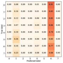
(a) Noisy Baseline $\to$
Maya Constant (12%)

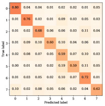
(b) Maya Constant $\to$
Maya Constant (67%)

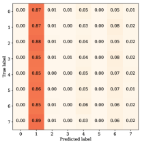
(c) Noisy Baseline $\to$
Maya Gaussian Sinusoid (13%)

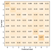
(d) Maya Gaussian Sinusoid $\to$ Maya Gaussian Sinusoid (20%)

Figure 5. Confusion matrices for a machine learning attack to identify the active application from power signals. The figures are labeled in the format: Train dataset $\to$ Test dataset and the average accuracy is in parenthesis. Higher fractions are in darker squares.

From each trace, we extract multiple segments of 15,000 RAPL measurements, and average the 5 consecutive measurements in each segment to remove effects of noise. This reduces each segment length to 3,000. Then, we convert the values in the segment into one-hot representation by quantizing the values into one of 10 levels encoded in one-hot format. This gives us 30,000-long samples that we feed into a classifier. Among the samples from all traces, we use 60% of them for training, 20% for validation, and leave 20% as the test set.

Our classifier is a multilayer perceptron neural network with two hidden ReLU layers of dimensions 1,500 and 600. The output layer uses Logsoftmax and has 8 nodes, corresponding to the 8 applications we classify. With this model, we achieve a training accuracy of 99%, and validation and test accuracies of 92%.

2. Detecting the Application Data: This attack is used to infer the differences in data that a given application uses – such as the websites accessed by a browser, or the videos processed by an encoder. This is also a common attack described in multiple works (Yan et al., 2015; Lifshits et al., 2018; Yang et al., 2017; Michalevsky et al., 2015; Wang et al., 2018). We implement this attack on Sys2 targeting the ffmpeg video encoding application (FFmpeg Developers, 2016). We use three videos saved in raw format: tractor, riverbed and wind. They are commonly used for video testing (Xiph.org Video Test Media, [n. d.]). We transcode each video with x264 compression using ffmpeg and record the power trace. Since the power consumed by video encoding depends on the content of the frames, each video has a distinct power pattern.

We collect the power traces from 300 runs of encoding each video with different frequency and idle activity levels. Next, we choose multiple windows of 1,000 measurements from each trace. As with the previous attack, we average 5 consecutive measurements and use on-hot encoding to obtain samples that are 2,000 values long.

The classifier for this attack is also a multilayer perceptron neural network with two hidden ReLU layers of dimensions 100 and 40. The output layer uses Logsoftmax and has 3 nodes corresponding to the 3 videos we classify. With this model, we achieve training, validation and test accuracies of 99%.

3. Adaptive Attacks: We consider an advanced scenario where the attacker records the distorted power traces of applications when Maya is running, and knows which application is running. She then trains models to perform the previous attacks. The data collection and model training is the same as described above.

6.2. Signal Processing Analysis

In addition to the machine learning attacks, we analyze Maya’s distortion using the following signal processing metrics.

1. Signal Averaging: Averaging multiple power signals removes random noise in the signals, allowing attackers to detect even small changes. We test this using signal averaging analysis on Sys1. For each application, we collect three sets of 1,000 noisy power signals with: (i) no Maya, (ii) Maya Constant, and (iii) Maya Gaussian Sinusoid. When Maya is not used, noise is created by changing frequency and idle activity. Then, we average the signals for each application and analyze the distribution of values in the averaged signals. Effective obfuscation would cause the values in the averaged traces to be distributed in the same manner across applications.

2. Change Detection: This is a signal processing technique used to identify times when the properties of a signal change. The properties can be the signal mean, variance, edges, or fourier coefficients. We use a standard Change Point Detection algorithm (MathWorks, [n. d.]) to compare the change points found in the baseline and in the re-shaped signals on Sys2.

7. Evaluating Maya

7.1. Evading Machine Learning Attacks

Application Detection Attack: Figure 5 shows the confusion matrices for performing the application detection attack and its adaptive variant on Sys1. The rows of the matrix correspond to the true labels of the traces and the columns are the predicted labels by the machine learning models. The 8 applications we detect are numbered from 0 to 7. A cell in the i^th row and j^th column of the matrix lists the fraction of traces belonging to label i that were classified as j. Values close to 1 along the diagonal indicate accurate prediction. We use Baseline to refer to the environment without Maya, and Obfuscated to refer when Maya runs.

Recall that the model trained on Noisy Baseline signals can classify unobfuscated signals with 92% accuracy. When this classifier is applied to signals produced when Maya runs with a Constant mask, the accuracy drops to 12% (average of the diagonal values in Figure 5a). However, when an advanced attacker trains on the obfuscated traces, the classification accuracy is 67% (Figure 5b).

The poor security offered by a Constant mask in the advanced attack is due to two reasons. First, it cannot hide the natural power variations of an application as described in Section 4.3. Second, the power signals of an application with a Constant mask are similar across multiple runs. Hence, a Constant mask is ineffective at preventing information leakage.

Next, consider the Gaussian Sinusoid mask. When a Noisy Baseline-trained classifier is used, the accuracy is 13% (Figure 5c). Even in an Adaptive attack that trains on the obfuscated traces, the classification accuracy is only 20% (Figure 5d). This indicates an excellent obfuscation, considering that the random-chance of guessing the correct application is 13%. The Gaussian Sinusoid introduces several types of variation in the power signals, effectively eliminating any original patterns. Moreover, each run with this mask generates a new form. Therefore, there is no common pattern between different runs that a machine learning module could learn.

Video Data Detection Attack: Figure 6 shows the confusion matrices for the attack that identifies the video being encoded on Sys2. Recall that the attack has to choose among one of three videos for each power trace. The classifier trained on baseline signals had a 99% test accuracy in predicting the video from the baseline traces. The classification accuracy when using this model on signals with Maya’s Constant mask is 21% (Figure 6a). However, the accuracy rises to 79% when the attacker is able to train with the power signals generated by Maya using the constant mask (Figure 6b).

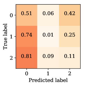
(a) Noisy Baseline $\to$
Maya Constant (21%)

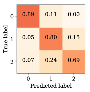
(b) Maya Constant $\to$ Maya Constant (79%)

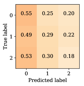
(c) Noisy Baseline $\to$ Maya Gaussian Sinusoid (34%)

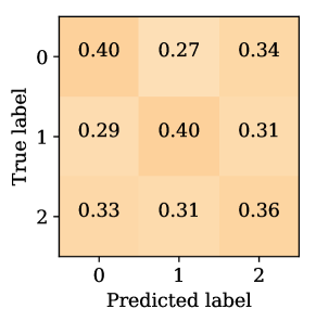
(d) Maya Gaussian Sinusoid $\to$ Maya Gaussian Sinusoid (39%)

Figure 6. Confusion matrices for a machine learning attack to identify the video being encoded. The figures are labeled as in Figure 5.

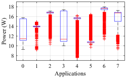
(a) Noisy Baseline

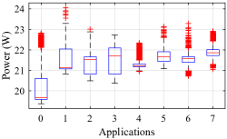
(b) Maya Constant

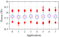
(c) Maya Gaussian Sinusoid

Figure 7. Summary statistics of the average of 1,000 signals. The Y axis of each chart is drawn to a different scale.

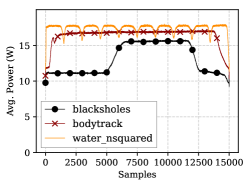
(a) Noisy Baseline

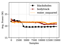
(b) Maya Constant

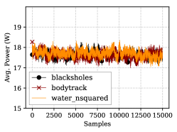
(c) Maya Gaussian Sinusoid

Figure 8. Average of 1,000 signals over time samples. The Y axis of each chart is drawn to a different scale.

When the Gaussian Sinusoid mask is used, the classification accuracy when using the Noisy Baseline-trained model is 34% (Figure 6c). Even when the attacker trains with obfuscated traces, the classification accuracy is only 39%(Figure 6d). This is a high degree of obfuscation because the random-chance of assigning the correct video to a power signal is 33%.

Overall, the results from the machine learning-based attacks establish that Maya with the Gaussian Sinusoid mask is successful in falsifying pattern recognition attacks. Maya’s strength is highlighted when it resisted the attacks where the attacker could record thousands of signals generated from Maya. This comes from using an effective mask (Gaussian Sinusoid) and a control-theory controller that keeps power close to the mask. Finally, the results also show the Constant mask to be ineffective because it does not have all the needed traits of a mask.

7.2. Signal Processing Analysis

Signal Averaging: Figure 7 shows the box plots of value distribution in the averaged traces from Sys1 with the Noisy Baseline, Maya Constant mask, and Maya Gaussian Sinusoid mask. The applications are labeled on the horizontal axis from 0 to 7. There is a box plot for each application. Each box shows the 25^th and 75^th percentile values for the application. The line inside the box is the median value. The whiskers of the box extend up to values not considered as statistical outliers. The statistical outliers are shown by a tail of ‘+’ markers. Note that the Y axis on the three charts is different – Figures 7b and 7c have a magnified view of the values for legibility.

With the Noisy Baseline, the average trace of each application has a distinct distribution of values, leaving a fingerprint of that application. With a Constant mask, the median values of the applications are closer than they were with the Baseline. The lengths of the boxes do not differ as much as they did with the Baseline. Unfortunately, each application has a different statistical fingerprint sufficient to distinguish it from the others.

Finally, with Maya Gaussian Sinusoid mask, the distributions are near-identical. This is because the patterns in each run are not correlated with those in other runs. Therefore, averaging multiple Maya signals cancels out the patterns — simply leaving a constant-like value with small variance. Hence, the median, mean, variance, and the distribution of the samples are very close. Note that the resolution of this data is 0.01W, indicating a high degree of obfuscation.

To highlight the differences further, Figure 8 shows the averaged signals of three applications over timesteps for the Noisy Baseline, Maya Constant and Maya Gaussian Sinusoid. Again, the Y axis for Figures 8b and 8c is magnified for legibility. With Noisy Baseline, after the noise is removed by the averaging effect, the patterns in the averaged signals of each application are clearly visible. Further, these patterns are different for each application.

When the Constant mask is used, the magnitude of the variation is lower, but the lines are not identical across applications. The pattern of blackscholes is clearly visible.

With the Gaussian Sinusoid mask, the average signal of an application has only a small variance, and is close to the average signals of the other applications. As a result, the average traces of different applications are indistinguishable, and do not resemble the baseline at all. This results in the highest degree of obfuscation.

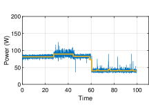
(a)

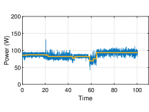
(b)

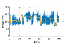
(c)

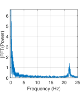
(a) Noisy Baseline

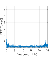
(b) Maya Constant

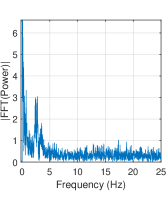
(c) Maya Gaussian Sinusoid

Figure 9. Change point detection in blackscholes on Sys2. The top row shows the time-domain signals, along with the detected phases. The bottom row shows the frequency-domain signals.

Change Point Detection: We present the highlights of this analysis using blackscholes on Sys2. We monitor the execution for 100 s, even if the application completes before 100 s. Figure 9 shows the power signals in the time and frequency domains for blackscholes with the Noisy Baseline, Maya Constant, and Maya Gaussian Sinusoid. The time-domain plots also show the detected phases from the change point algorithm.

In the Noisy Baseline (Figure 9a), the difference between the different phases is less visible due to interference from the idle threads. Nonetheless, the algorithm detects four major phases. They correspond to the sequential, parallel, sequential, and fully idle activity, respectively. The sudden changes between phases can be seen as a small spike in the FFT tail of this signal.

Figure 9b shows blackscholes with a Constant mask. Change point analysis reveals changes in the signal at 20s, 40s and 60s, yielding four phases. These phases can be related directly to those in the Baseline signal because the Constant mask does not introduce artificial changes. The change in signal variance between these phases is visible from the time series. Also, the FFT tail has a small spike at the same location as with the Baseline. As a result, the attacker can easily identify this signal.

Figure 9c shows the behavior with the Gaussian Sinusoid mask. Change point analysis detects several instances of phase change, but these are all artificial. Notice that the FFT of this signal is different from the Baseline FFT, eliminating any identity of the application. Finally, it is also not possible to infer when the application execution is complete. Specifically, the application actually completed around 55 s, but the power signal has no distinguishing change at that time.

7.3. Effectiveness of a Control-Theory Controller

Figure 10 shows the target power given by a Maya Gaussian Sinusoid mask generator during one execution of blackscholes on Sys1 (a), and the actual power that was measured from the computer (b). It can be seen that the control-theory controller is effective at making the measured power appear close to the target mask. This is thanks to the advantages of using a MIMO control theoretic controller. Indeed, this accurate tracking is what helps Maya in effectively re-shaping the system’s power and hide application activity.

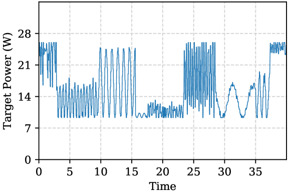
(a) Ideal target power given by the mask.

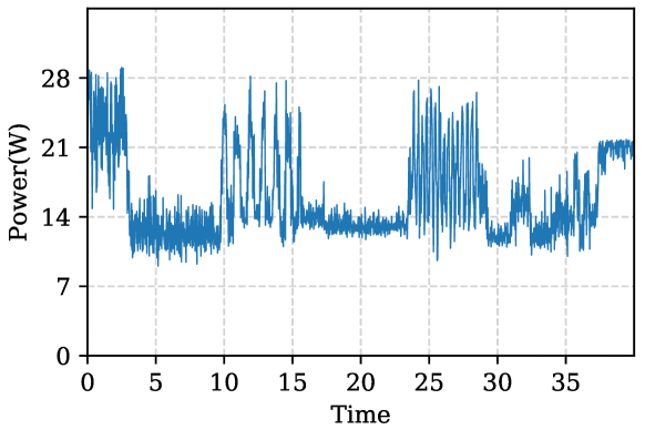
(b) Measured power from the system.

Figure 10. Target and measured powers for a run of blackscholes with Maya Gaussian Sinusoid on Sys1, showing the high-fidelity power-shaping with control theory.

7.4. Overheads and Power-Performance Impact

Finally, we examine the overheads and the power-performance impact of Maya.

Overheads of Maya: The controller reads one output, sets three inputs and, it can be shown, has a state vector $x(T)$ that is 11-element long (Equation 1). Therefore, the controller needs less than 1 KB of storage. At each invocation, it performs $\approx$200 fixed-point operations to make a decision. This completes within one $\mu$s.

The Mask Generator requires (pseudo) random numbers from a Gaussian distribution to compute the mask (Equation 4). It also needs another set of random numbers to set the properties of the Gaussian distribution and the Sinusoid. In our implementation, we use a software library that takes less than 10 $\mu$s to generate all our random numbers. For a hardware implementation, there are off-the-shelf hardware instructions and IP modules to obtain these random numbers in sub-$\mu$s (John M, 2018; Intel, 2017).

Maya needs few resources to control the system, making Maya attractive for both hardware and software implementations. The primary bottlenecks in our implementation were the sensing and actuation latencies, which are in the ms time scale.

Application-Level Impact: We run the PARSEC and SPLASH2x applications on Sys1 and Sys2, with and without Maya, to measure the power and performance overheads. Our Baseline configuration runs at the highest available frequency without interference from the idle threads or the balloon program. It offers no security. We also evaluate the Noisy Baseline design, in which the system runs with a random DVFS level and percentage of idle activity.

Figure 11 shows the power and execution time of the Noisy Baseline, Maya Constant and Maya Gaussian Sinusoid environments normalized to that of the high-performance Baseline. From Figure 11a, we see that the average power consumed by the applications with the three environments is 35%, 41%, and 29% lower than that of the high performance Baseline, respectively. The power is lower due to the idle threads and low DVFS values that appear in these environments.

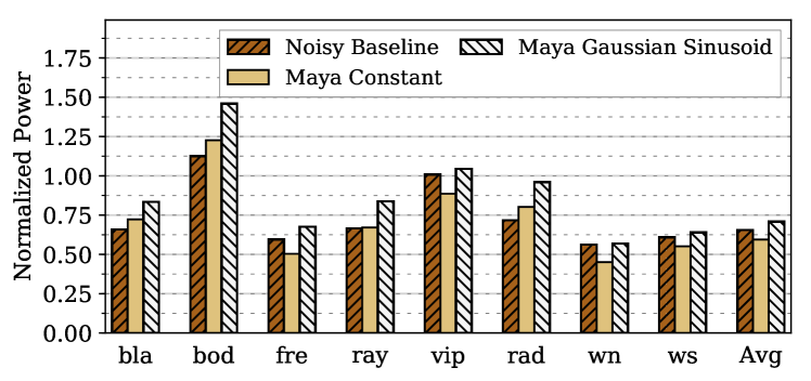
(a) Power

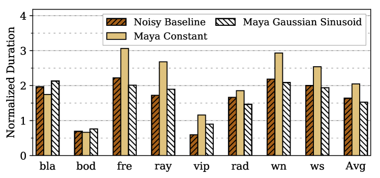
(b) Execution Time

Figure 11. Overheads of our environments on Sys1 relative to a high-performance insecure Baseline.

Figure 11b shows the normalized execution times with the Noisy Baseline, Maya Constant, and Maya Gaussian Sinusoid environments. These environments have, on average, performance slowdowns of 63%, 100% and 50% respectively, over the Baseline. Maya Constant uses a single power target that is lower than the maximum power at which Baseline runs. Therefore, its performance is the worst. On the other hand, Maya Gaussian Sinusoid spans multiple power levels in the available range, allowing applications to run at higher power occasionally. As a result, execution times are relatively better. Maya Gaussian Sinusoid also has a better performance than Noisy Baseline and offers high security.

It can be shown that the power and performance overheads of our environments in Sys2 are similar to those in Sys1 shown in Figure 11. This shows that our methodology is robust across different machine configurations.

One approach to reduce the slowdown from Maya is to enable obfuscation only on demand. Authenticated users or secure applications can activate Maya before commencing a secure-sensitive task, and stop Maya once the task is complete. While this approach gives away the information that a secure task is being run, at least does not slow down all applications.

7.5. Overall Remarks

Using machine learning-based attacks and signal analysis, we showed how the Maya Gaussian Sinusoid mask can obfuscate power signals from a computer. Maya’s security comes from an effective mask, and from the control-theoretic controller that can shape the computer’s power into the given mask. We implemented Maya on two different machines without modifying the controller or the mask generator, demonstrating our proposal’s robustness, security and ease of deployment on existing computers.

8. Related Work

Power, temperature, and EM emissions from a computer are a set of physical side channels that have been used by many attackers to compromise security (Kocher et al., 2011; Zhou and Feng, 2005; Zhang et al., 2016). Kocher et al. (Kocher et al., 2011) give a detailed overview of attacks exploiting power signals with Simple Power analysis (SPA) and Differential Power Analysis (DPA).

Machine Learning (ML) is commonly-used to perform power analysis attacks. Using ML, Yan et al. developed an attack to identify the running application, login screens and the number of keystrokes typed by the user (Yan et al., 2015). Lifshits et al. considered malicious smart batteries and demonstrated another attack that predicted the character of a keystroke and user’s personal information such as browser, camera, and location activity (Lifshits et al., 2018). Yang et al. snooped the power drawn by a mobile phone from a public USB charging booth to predict the user’s browser activity. Hlavacs et al. showed that the virtual machines running on a server could be identified using power signals (Hlavacs et al., 2011). Finally, Wei et al. used ML to detect malware from power signals (Wei et al., 2019).

Other attacks are even more sophisticated. Michalevsky et al. developed a malicious smartphone application that could track the user’s location using OS-level power counters, without reading the GPS module (Michalevsky et al., 2015). Schellenberg et al. showed how malicious on-board modules can measure another chip’s power activity (Schellenberg et al., 2018).

As power, temperature, and EM emissions are correlated, attackers used temperature and EM measurements to identify application activity (Genkin et al., 2016; Genkin et al., 2014; Alam et al., 2018; Callan et al., 2015; Kasper et al., 2009; Wang et al., 2018). These attacks have targeted many environments, like smart cards, mobile systems, laptops, and IoT devices. Recently, Masti et al. showed how temperature can be used to identify another core’s activity in multicores (Masti et al., 2015). This broadens the threat from physical side channels because attackers can read EM signals from a distance, or measure temperature through co-location, even when the system does not support per-core power counters.

Several countermeasures against power side channels have been proposed (Zhang et al., 2016; Tiri and Verbauwhede, 2005; Saputra et al., 2003; Yang et al., 2005; Das et al., 2017; Kocher et al., 2011; Yang et al., 2012; Avirneni and Somani, 2014). They usually operate along one of two principles: keep power consumption invariant to any activity (Tiri and Verbauwhede, 2005; Saputra et al., 2003; Ratanpal et al., 2004; Yu et al., 2015; Das et al., 2017), or make power consumption noisy such that the impact of application activity is lost (Kocher et al., 2011; Zhang et al., 2016). A common approach is to randomize DVFS using special hardware (Yang et al., 2012; Avirneni and Somani, 2014; Yang et al., 2012). Avirneni and Somani also propose new circuits for randomizing DVFS, and change voltage and frequency independently (Avirneni and Somani, 2014).

Baddam and Zwolinski showed that randomizing DVFS is not a viable defense because attackers can identify clock frequency changes through high-resolution power traces (Baddam and Zwolinski, 2007). Yang et al. proposed using random task scheduling at the OS level in addition to new hardware for randomly setting the processor frequency and clock phase (Yang et al., 2018). Real et al. showed that simple approaches to introduce noise or empty activity into the system can be filtered out (Real et al., 2008).

Trusted execution environments like Intel SGX (McKeen et al., 2013) or ARM Trustzone (ARM, 2009) can sandbox the architectural events of applications. However, they do not establish boundaries for physical signals. One approach for power side channel isolation is blinking (Althoff et al., 2018), where a circuit is temporarily cut-off from the outside and is run with a small amount of energy stored inside itself (Althoff et al., 2018).

To the best of our knowledge, Maya is the first defense against power side channels that uses control theory.

9. Conclusions

This paper presented a simple and effective solution against power side channels. The idea, called Maya, is to use a controller from control theory to distort, in an application-transparent way, the power consumed by an application – so that the attacker cannot obtain information. With control theory techniques, the controller can keep outputs close to desired targets even when runtime conditions change unpredictably. Then, by changing these targets appropriately, Maya makes the power signal appear to carry activity information which, in reality, is unrelated to the program. Maya controllers can be implemented in privileged software or in simple hardware. In this paper, we implemented Maya on two multiprocessor machines using OS threads, and showed that it is very effective at falsifying application activity.

References

- (1)
- and ([n. d.]) [n. d.]. Power Profiles for Android. https://source.android.com/devices/tech/power/. Android Open Source Project.
- Alam et al. (2018) Monjur Alam, Haider Adnan Khan, Moumita Dey, Nishith Sinha, Robert Callan, Alenka Zajic, and Milos Prvulovic. 2018. One&Done: A Single-Decryption EM-Based Attack on OpenSSL’s Constant-Time Blinded RSA. In USENIX Security. USENIX Association, Baltimore, MD, 585–602. https://www.usenix.org/conference/usenixsecurity18/presentation/alam
- Althoff et al. (2018) A. Althoff, J. McMahan, L. Vega, S. Davidson, T. Sherwood, M. Taylor, and R. Kastner. 2018. Hiding Intermittent Information Leakage with Architectural Support for Blinking. In ISCA. 638–649. https://doi.org/10.1109/ISCA.2018.00059
- ARM ([n. d.]a) ARM. [n. d.]a. ARM® Cortex®-A15 Processor. https://www.arm.com/products/processors/cortex-a/cortex-a15.php.
- ARM ([n. d.]b) ARM. [n. d.]b. ARM® Cortex®-A7 Processor. https://www.arm.com/products/processors/cortex-a/cortex-a7.php.
- ARM (2009) ARM. 2009. ARM Security Technology Building a Secure System using TrustZone Technology. http://infocenter.arm.com/help/topic/com.arm.doc.prd29-genc-009492c/PRD29-GENC-009492C_trustzone_security_whitepaper.pdf.
- Avirneni and Somani (2014) N. D. P. Avirneni and A. K. Somani. 2014. Countering Power Analysis Attacks UsingReliable and Aggressive Designs. IEEE Trans. Comput. 63, 6 (jun 2014), 1408–1420. https://doi.org/10.1109/TC.2013.9
- Baddam and Zwolinski (2007) K. Baddam and M. Zwolinski. 2007. Evaluation of Dynamic Voltage and Frequency Scaling as a Differential Power Analysis Countermeasure. In VLSID. 854–862. https://doi.org/10.1109/VLSID.2007.79
- Beck et al. (2018) Noah Beck, Sean White, Milam Paraschou, and Samuel Naffziger. 2018. “Zeppelin”: An SoC for Multichip Architectures. In ISSCC.
- Benhani and Bossuet (2018) E. M. Benhani and L. Bossuet. 2018. DVFS as a Security Failure of TrustZone-enabled Heterogeneous SoC. In International Conference on Electronics, Circuits and Systems (ICECS). 489–492. https://doi.org/10.1109/ICECS.2018.8618038
- Bienia et al. (2008) Christian Bienia, Sanjeev Kumar, Jaswinder Pal Singh, and Kai Li. 2008. The PARSEC Benchmark Suite: Characterization and Architectural Implications. In PACT.
- Bukasa et al. (2018) Sebanjila Kevin Bukasa, Ronan Lashermes, Hélène Le Bouder, Jean-Louis Lanet, and Axel Legay. 2018. How TrustZone Could Be Bypassed: Side-Channel Attacks on a Modern System-on-Chip. In Information Security Theory and Practice, Gerhard P. Hancke and Ernesto Damiani (Eds.). Springer International Publishing, Cham, 93–109.
- Callan et al. (2015) R. Callan, N. Popovic, A. Daruna, E. Pollmann, A. Zajic, and M. Prvulovic. 2015. Comparison of electromagnetic side-channel energy available to the attacker from different computer systems. In 2015 IEEE International Symposium on Electromagnetic Compatibility (EMC). 219–223. https://doi.org/10.1109/ISEMC.2015.7256162
- Das et al. (2017) D. Das, S. Maity, S. B. Nasir, S. Ghosh, A. Raychowdhury, and S. Sen. 2017. High efficiency power side-channel attack immunity using noise injection in attenuated signature domain. In HOST. 62–67. https://doi.org/10.1109/HST.2017.7951799
- FFmpeg Developers (2016) FFmpeg Developers. 2016. ffmpeg tool. http://ffmpeg.org/.
- Genkin et al. (2016) Daniel Genkin, Lev Pachmanov, Itamar Pipman, Eran Tromer, and Yuval Yarom. 2016. ECDSA Key Extraction from Mobile Devices via Nonintrusive Physical Side Channels. In CCS (CCS ’16). ACM, New York, NY, USA, 1626–1638. https://doi.org/10.1145/2976749.2978353
- Genkin et al. (2014) Daniel Genkin, Itamar Pipman, and Eran Tromer. 2014. Get Your Hands Off My Laptop: Physical Side-Channel Key-Extraction Attacks on PCs. In Proceedings of the 16th International Workshop on Cryptographic Hardware and Embedded Systems — CHES 2014 - Volume 8731. Springer-Verlag, Berlin, Heidelberg, 242–260. https://doi.org/10.1007/978-3-662-44709-3_14
- Gu et al. (2013) Da-Wei Gu, Petko H. Petkov, and Mihail M. Konstantinov. 2013. Robust Control Design with MATLAB (2nd ed.). Springer.
- Hlavacs et al. (2011) H. Hlavacs, T. Treutner, J. Gelas, L. Lefevre, and A. Orgerie. 2011. Energy Consumption Side-Channel Attack at Virtual Machines in a Cloud. In International Conference on Dependable, Autonomic and Secure Computing. 605–612. https://doi.org/10.1109/DASC.2011.110
- Intel (2017) Intel. 2017. Random Number Generator IP Core User Guide . https://www.intel.com/content/www/us/en/programmable/documentation/dmi1455632999173.html.
-
John M (2018)
John M. 2018.
Intel Digital Random Number Generator (DRNG)
Software Implementation Guide.
https://software.intel.com/en-us/articles/intel-digital-random-number-generator-drng-software-
implementation-guide. - Kasper et al. (2009) Timo Kasper, David Oswald, and Christof Paar. 2009. EM Side-Channel Attacks on Commercial Contactless Smartcards Using Low-Cost Equipment. In Information Security Applications, Heung Youl Youm and Moti Yung (Eds.). Springer Berlin Heidelberg, Berlin, Heidelberg, 79–93.
- Kocher et al. (1999) Paul Kocher, Joshua Jaffe, and Benjamin Jun. 1999. Differential power analysis. In Annual International Cryptology Conference. Springer, 388–397.
- Kocher et al. (2011) Paul Kocher, Joshua Jaffe, Benjamin Jun, and Pankaj Rohatgi. 2011. Introduction to differential power analysis. Journal of Cryptographic Engineering 1, 1 (01 Apr 2011), 5–27. https://doi.org/10.1007/s13389-011-0006-y
- Lezcano ([n. d.]) Daniel Lezcano. [n. d.]. Idle Injection. https://www.linuxplumbersconf.org/event/2/contributions/184/attachments/42/49/LPC2018_-_Thermal_-_Idle_injection_1.pdf. Linux Plumbers Conference, 2018.
- Lifshits et al. (2018) Pavel Lifshits, Roni Forte, Yedid Hoshen, Matt Halpern, Manuel Philipose, Mohit Tiwari, and Mark Silberstein. 2018. Power to peep-all: Inference Attacks by Malicious Batteries on Mobile Devices. PoPETs 2018, 4 (2018), 141–158. https://content.sciendo.com/view/journals/popets/2018/4/article-p141.xml
- Ljung (1999) Lennart Ljung. 1999. System Identification : Theory for the User (2 ed.). Prentice Hall PTR, Upper Saddle River, NJ, USA.
- Masti et al. (2015) Ramya Jayaram Masti, Devendra Rai, Aanjhan Ranganathan, Christian Müller, Lothar Thiele, and Srdjan Capkun. 2015. Thermal Covert Channels on Multi-core Platforms. In USENIX Security. USENIX Association, Washington, D.C., 865–880. https://www.usenix.org/conference/usenixsecurity15/technical-sessions/presentation/masti
- MathWorks ([n. d.]) MathWorks. [n. d.]. Find abrupt changes in signal. https://www.mathworks.com/help/signal/ref/findchangepts.html. Accessed: April, 2019.
- McKeen et al. (2013) Frank McKeen, Ilya Alexandrovich, Alex Berenzon, Carlos V. Rozas, Hisham Shafi, Vedvyas Shanbhogue, and Uday R. Savagaonkar. 2013. Innovative Instructions and Software Model for Isolated Execution. In Proceedings of the 2Nd International Workshop on Hardware and Architectural Support for Security and Privacy (HASP ’13). ACM, New York, NY, USA, Article 10, 1 pages. https://doi.org/10.1145/2487726.2488368
- Michalevsky et al. (2015) Yan Michalevsky, Aaron Schulman, Gunaa Arumugam Veerapandian, Dan Boneh, and Gabi Nakibly. 2015. PowerSpy: Location Tracking Using Mobile Device Power Analysis. In USENIX Security. USENIX Association, Washington, D.C., 785–800. https://www.usenix.org/conference/usenixsecurity15/technical-sessions/presentation/michalevsky
- Pandruvada ([n. d.]) Srinivas Pandruvada. [n. d.]. Running Average Power Limit – RAPL. https://01.org/blogs/2014/running-average-power-limit--rapl. Published: June, 2014.
- Pothukuchi et al. (2016) Raghavendra Pradyumna Pothukuchi, Amin Ansari, Petros Voulgaris, and Josep Torrellas. 2016. Using Multiple Input, Multiple Output Formal Control to Maximize Resource Efficiency in Architectures. In ISCA.
- Ratanpal et al. (2004) Girish B. Ratanpal, Ronald D. Williams, and Travis N. Blalock. 2004. An On-Chip Signal Suppression Countermeasure to Power Analysis Attacks. IEEE Trans. Dependable Secure Comput. 1, 3 (jul 2004), 179–189. https://doi.org/10.1109/TDSC.2004.25
- Real et al. (2008) D. Real, C. Canovas, J. Clediere, M. Drissi, and F. Valette. 2008. Defeating classical Hardware Countermeasures: a new processing for Side Channel Analysis. In DATE. 1274–1279. https://doi.org/10.1109/DATE.2008.4484854
- Rotem (2015) Efraim Rotem. 2015. Intel Architecture, Code Name Skylake Deep Dive: A New Architecture to Manage Power Performance and Energy Efficiency. Intel Developer Forum.
- Rotem et al. (2012) E. Rotem, A. Naveh, D. Rajwan, A. Ananthakrishnan, and E. Weissmann. 2012. Power-Management Architecture of the Intel Microarchitecture Code-Named Sandy Bridge. MICRO 32, 2 (mar 2012), 20–27. https://doi.org/10.1109/MM.2012.12
- Saputra et al. (2003) H. Saputra, N. Vijaykrishnan, M. Kandemir, M. J. Irwin, R. Brooks, S. Kim, and W. Zhang. 2003. Masking the energy behavior of DES encryption [smart cards]. In DATE. 84–89. https://doi.org/10.1109/DATE.2003.1253591
- Schellenberg et al. (2018) Falk Schellenberg, Dennis R. E. Gnad, Amir Moradi, and Mehdi B. Tahoori. 2018. Remote Inter-chip Power Analysis Side-channel Attacks at Board-level. In ICCAD (ICCAD ’18). ACM, New York, NY, USA, Article 114, 7 pages. https://doi.org/10.1145/3240765.3240841
- Shao and Brooks (2013) Y. S. Shao and D. Brooks. 2013. Energy characterization and instruction-level energy model of Intel’s Xeon Phi processor. In ISLPED. 389–394. https://doi.org/10.1109/ISLPED.2013.6629328
- Skogestad and Postlethwaite (2005) Sigurd Skogestad and Ian Postlethwaite. 2005. Multivariable Feedback Control: Analysis and Design. John Wiley & Sons.
- Tiri and Verbauwhede (2005) K. Tiri and I. Verbauwhede. 2005. Design method for constant power consumption of differential logic circuits. In DATE. 628–633 Vol. 1. https://doi.org/10.1109/DATE.2005.113
- Toprak-Deniz et al. (2014) Z. Toprak-Deniz, M. Sperling, J. Bulzacchelli, G. Still, R. Kruse, Seongwon Kim, D. Boerstler, T. Gloekler, R. Robertazzi, K. Stawiasz, T. Diemoz, G. English, D. Hui, P. Muench, and J. Friedrich. 2014. 5.2 Distributed system of digitally controlled microregulators enabling per-core DVFS for the POWER8TM microprocessor. In ISSCC. 98–99. https://doi.org/10.1109/ISSCC.2014.6757354
- van de Ven and Pan ([n. d.]) Arjan van de Ven and Jacob Pan. [n. d.]. Intel Powerclamp Driver. https://www.kernel.org/doc/Documentation/thermal/intel_powerclamp.txt. Last modified: April, 2017.
- Vasilakis (2015) Evangelos Vasilakis. 2015. An instruction level energy characterization of arm processors. https://www.ics.forth.gr/carv/greenvm/files/tr450.pdf.
- Wang et al. (2018) Xiao Wang, Quan Zhou, Jacob Harer, Gavin Brown, Shangran Qiu, Zhi Dou, John Wang, Alan Hinton, Carlos Aguayo Gonzalez, and Peter Chin. 2018. Deep learning-based classification and anomaly detection of side-channel signals. In Proc. SPIE 10630, Cyber Sensing. https://doi.org/10.1117/12.2311329
- Wei et al. (2019) S. Wei, A. Aysu, M. Orshansky, A. Gerstlauer, and M. Tiwari. 2019. Using Power-Anomalies to Counter Evasive Micro-Architectural Attacks in Embedded Systems. In HOST. 111–120. https://doi.org/10.1109/HST.2019.8740838
- Xiph.org Video Test Media ([n. d.]) Xiph.org Video Test Media. [n. d.]. derf’s collection. https://media.xiph.org/.
- Yan et al. (2015) Lin Yan, Yao Guo, Xiangqun Chen, and Hong Mei. 2015. A Study on Power Side Channels on Mobile Devices. In Proceedings of the 7th Asia-Pacific Symposium on Internetware (Internetware ’15). ACM, New York, NY, USA, 30–38. https://doi.org/10.1145/2875913.2875934
- Yang et al. (2018) Jianwei Yang, Fan Dai, Jielin Wang, Jianmin Zeng, Zhang Zhang, Jun Han, and Xiaoyang Zeng. 2018. Countering power analysis attacks by exploiting characteristics of multicore processors. IEICE Electronics Express advpub (2018). https://doi.org/10.1587/elex.15.20180084
- Yang et al. (2017) Q. Yang, P. Gasti, G. Zhou, A. Farajidavar, and K. S. Balagani. 2017. On Inferring Browsing Activity on Smartphones via USB Power Analysis Side-Channel. IEEE Trans. Inf. Forensics Security 12, 5 (may 2017), 1056–1066. https://doi.org/10.1109/TIFS.2016.2639446
- Yang et al. (2012) Shengqi Yang, Pallav Gupta, Marilyn Wolf, Dimitrios Serpanos, Vijaykrishnan Narayanan, and Yuan Xie. 2012. Power Analysis Attack Resistance Engineering by Dynamic Voltage and Frequency Scaling. ACM Trans. Embed. Comput. Syst. 11, 3, Article 62 (sep 2012), 16 pages. https://doi.org/10.1145/2345770.2345774
- Yang et al. (2005) Shengqi Yang, Wayne Wolf, Narayanan Vijaykrishnan, Dimitrios N. Serpanos, and Yuan Xie. 2005. Power attack resistant cryptosystem design: A dynamic voltage and frequency switching approach. In DATE. IEEE, 64–69.
- Yu et al. (2015) Weize Yu, Orhun Aras Uzun, and Selçuk Köse. 2015. Leveraging On-chip Voltage Regulators As a Countermeasure Against Side-channel Attacks. In DAC (DAC ’15). ACM, New York, NY, USA, Article 115, 6 pages. https://doi.org/10.1145/2744769.2744866
- Zhang et al. (2016) Lu Zhang, Luis Vega, and Michael Taylor. 2016. Power Side Channels in Security ICs: Hardware Countermeasures. arXiv:cs.CR/1605.00681
- Zhou and Feng (2005) YongBin Zhou and DengGuo Feng. 2005. Side-Channel Attacks: Ten Years After Its Publication and the Impacts on Cryptographic Module Security Testing. http://eprint.iacr.org/2005/388 zyb@is.iscas.ac.cn 13083 received 27 Oct 2005.