SOLITON TRANSMUTATIONS IN KDV—BURGERS LAYERED MEDIA

Abstract.

We study the behavior of the soliton which, while moving in non-dissipative medium encounters a barrier with dissipation. The modelling included the case of a finite dissipative layer as well as a wave passing from a dissipative layer into a non-dissipative one and vice versa. New effects are presented in the case of numerically finite barrier on the soliton path: first, if the form of dissipation distribution has a form of a frozen soliton, the wave that leaves the dissipative barrier becomes a bi-soliton and a reflection wave arises as a comparatively small and quasi-harmonic oscillation. Second, if the dissipation is negative (the wave, instead of loosing energy, is pumped with it) the passed wave is a soliton of a greater amplitude and velocity. Third, when the travelling wave solution of the KdV-Burgers (it is a shock wave in a dissipative region) enters a non-dissipative layer this shock transforms into a quasi-harmonic oscillation known for the KdV.

Keywords: KdV- Burgers, non-homogeneous layered media, soliton, bi-soliton, shock wave.

1. Introduction

The behavior of solutions to the KdV - Burgers equation is a subject of various recent research, [1]–[6]; the present paper is a continuation of [2].

The generalized KdV-Burgers (KdV-B) equation

$$u_{t}(x,t)=\gamma(x)u_{xx}(x,t)+2u(x,t)u_{x}(x,t)+u_{xxx}(x,t).$$ (1)

It is related to the viscous and dispersive medium. The layered media consist of layers with both dispersion an dissipation (modelled by KdV-B) and layers without dissipation (KdV).

• $\gamma(x)=0\Rightarrow$ KdV $\Rightarrow$ travelling waves solutions (TWS) are solitons;

• $\gamma(x)=\mathrm{const}>0\Rightarrow$ KdV-Burgers $\Rightarrow$ TWS are shock waves.

Thus we consider the following possibilities for $\gamma(x)$.

1. The two-layer case: $\gamma(x)=\alpha(1-\theta(x))$, $\theta(x)=\mathrm{sign}(x)$ — the Heaviside step function; or $\gamma(x)=\alpha(1-\tanh(x))$, its smooth analog;

2. The three-layer case: $\gamma(x)=\alpha(\theta(x-\beta)-\theta(x+\beta))$, a $\Pi$-form density of viscosity, or $\gamma(x)=\alpha\mathop{\mathrm{sech}}\nolimits^{2}(\beta x)$, its smooth analog with (numerically) compact support.

Initial value-boundary problem for the KdV-Burgers :

$$u(x,0)=u_{0}(x,a,s)=6a^{2}\mathop{\mathrm{sech}}\nolimits^{2}(a(x+s)),\;u_{x}(\pm\infty,t)=0:$$ (2)

This is the initial placement of a soliton

$u_{0}(x,a,s)=\left.6a^{2}\mathop{\mathrm{sech}}\nolimits^{2}(4a^{3}t+a(x+s))\right|_{t=0}$ moving to the left.

For numerical computations $x\in[a,b]$ for appropriately large $a,\;b$.

2. Three layers case

2.1. $\Pi$ - type dissipation barrier

This case models a passage from non-dissipative half-space to another one passing through a dissipative layer (a process similar to a wave passing through an air-glass-air pile). We take $\gamma(x)=\alpha(\theta(x-\beta)-\theta(x+\beta))$ as a $\Pi$-form density of viscosity (the three-layer case) distribution function to present the layer separating these half-spaces.

Our experiments show that the initial soliton behaves as the one of the KdV at the right half-space and as a diminished soliton or a bi-soliton at the left one.

The process of transition is natural enough. The transient wave in a dissipative media looses energy and speed to become a lesser and slower solution at the left non-dissipative half-space; and a reflected wave is seen at the right half-space as it is shown at figures 1, 4. You may also see the 13.avi Maple-generated movie attached to this paper.

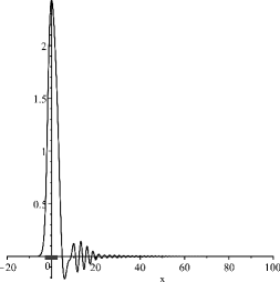
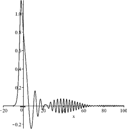
Figure 1. Left: Soliton ($a=1$) passing a thin viscose $\Pi$-type layer ($\alpha=2.5$, $\beta=2$); $t=1$
           Right: $t=3$

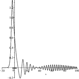
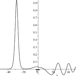
Figure 2. Left: Soliton ($a=1$) passing a thin viscose $\Pi$-type layer ($\alpha=2.5$, $\beta=2$); $t=5$.
           Right: Soliton (initially $a=1$) becomes that of $a=0.4$ after passing a thin viscose $\Pi$-type layer ($\alpha=6$, $\beta=2$); $t=50$.

The size of the reflected breather is connected, in particular, to the properties of the barrier $\alpha$ and $\beta$. So it may be of a practical use: for instance, measuring it one can judge whether the layer connecting two details is uniform at different points.

The natural question: is it possible to shut a soliton altogether using the dissipative layer? The absolute filter is impossible, but… see the figures 3, 4. You may also see the widePi.avi Maple-generated movie attached to this paper.

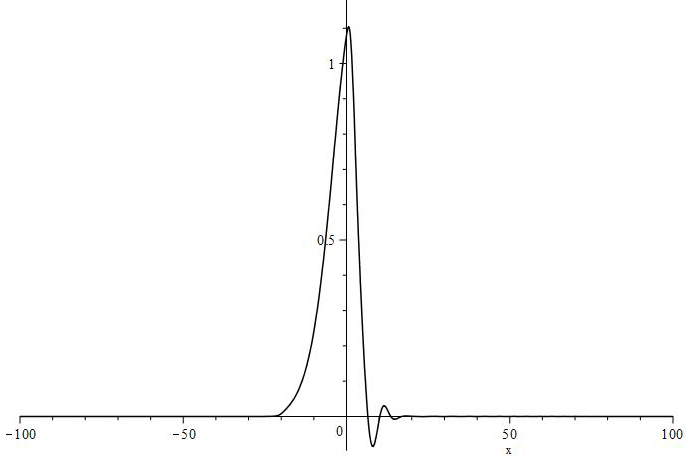
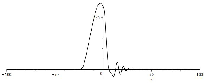
Figure 3. Left: Soliton ($a=0.5$) passing $\Pi$-type obstacle located at: $\mathbf{-20<x<0}$, $t=7$
           Right: $t=10$.

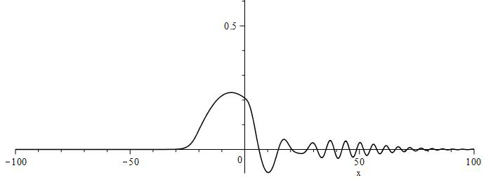
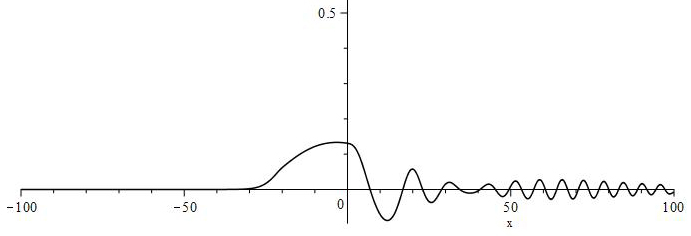
Figure 4. Left: Soliton ($a=0.5$) passing $\Pi$-type obstacle located at: $\mathbf{-20<x<0}$, $t=20$
           Right: $t=30$.

2.2. Soliton-form barrier

Since the barrier $\gamma(x)=\alpha\cosh^{-2}(\beta x)$ has a numerically compact support, the transition process is similar to that for the $\Pi$-type obstacle as it is illustrated by figures 5–9. You may also see the bi-2.avi Maple-generated movie attached to this paper.

For pictures in this subsection the equation is chosen in a different but equivalent form

$$u_{t}(x,t)=\gamma(x)u_{xx}(x,t)+6u(x,t)u_{x}(x,t)+u_{xxx}(x,t)$$ (3)

with $\gamma(x)=2\mathop{\mathrm{sech}}\nolimits^{2}(x)$

The solitons for the corresponding KdV, $u_{t}=+6u(x,t)u_{x}+u_{xxx}$, are of the form $\frac{1}{2}a^{2}\mathop{\mathrm{sech}}\nolimits^{2}(\frac{a}{2}(a^{2}t+x)+s)$.

Note that $\gamma(x)$ has a form of the soliton for $a=2,\;s=t=0$ but it is stationary, with zero velocity (a frozen soliton).

The transient wave becomes a bi-soliton — this effect is not observed as distinctly for different type barriers. Both peaks have the right ratioo of heights to velocities.

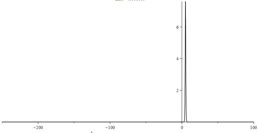
Figure 5. Soliton ($a=4$) passing a thin viscose layer $\gamma(x)=2\mathop{\mathrm{sech}}\nolimits^{2}(x)$, $t=0$

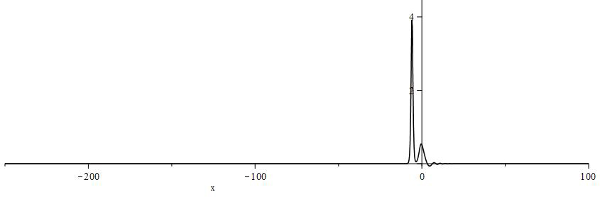
Figure 6. Soliton ($a=4$) passing a thin viscose layer $2\mathop{\mathrm{sech}}\nolimits^{2}(x)$, $t=1$.

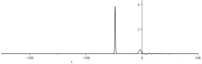
Figure 7. Soliton ($a=4$) passing a thin viscose layer $\gamma(x)=2\mathop{\mathrm{sech}}\nolimits^{2}(x)$, $t=5$

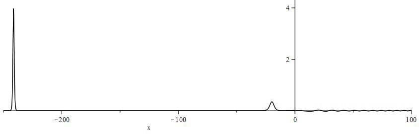
Figure 8. Soliton ($a=4$) passing a thin viscose layer $2\mathop{\mathrm{sech}}\nolimits^{2}(x)$, $t=30$. The refraction coefficient for the first peak is $k\approx\frac{8}{4}\approx 2$

2.3. Pumping area instead of dissipationone:

Invert the sign of $\gamma$ and look at soliton ($a=4$) crossing the ”pumping” area ($\gamma=-2\mathop{\mathrm{sech}}\nolimits^{2}(x)\ll 0$: the energy is not lost, but is acquired instead). The soliton comes out greater in amplitude and velocity; and the reflected wave gets a substantial impetus (figures 9–12). You may also see the bi-6.avi Maple-generated movie attached to this paper.

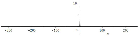
Figure 9. Soliton ($a=4$) at a thin negative-viscose layer $\gamma(x)=-2\mathop{\mathrm{sech}}\nolimits^{2}(x)$, $t=0$

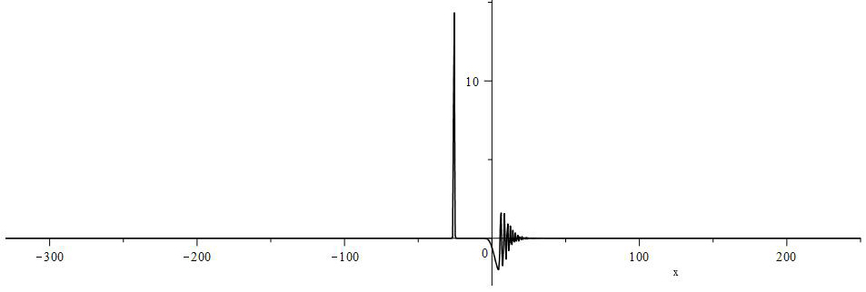
Figure 10. Soliton ($a=4$) passing a thin negative-viscose layer $-2\mathop{\mathrm{sech}}\nolimits^{2}(x)$, $t=0.7$.

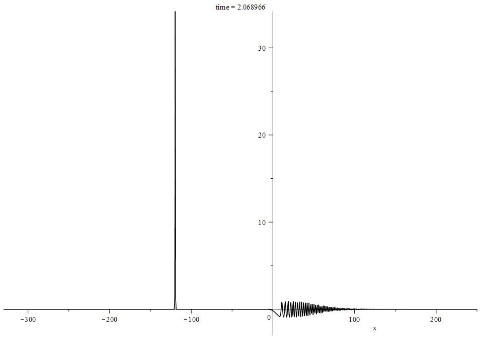
Figure 11. Soliton ($a=4$) passing a thin negative-viscose layer $-2\mathop{\mathrm{sech}}\nolimits^{2}(x)$, $t=2$.

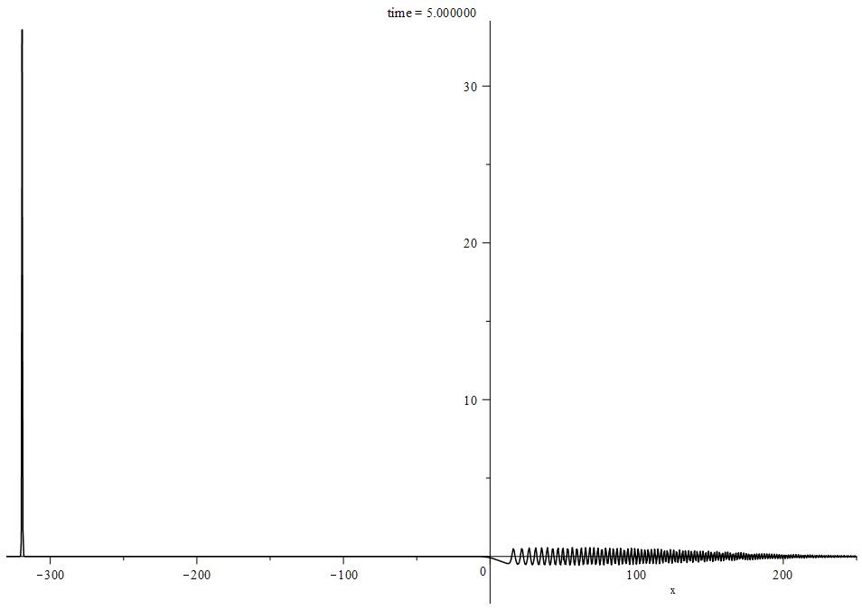
Figure 12. Soliton ($a=4$) passing a thin negative-viscose layer $-2\mathop{\mathrm{sech}}\nolimits^{2}(x)$, $t=5$.

3. Soliton in 2-layer medium

This case models a passage from a dissipative half-space to a non-dissipative one. We take $\gamma(x)=0.5(1+\theta(x))$ as a dissipation distribution function to present a single boundary separating these half-spaces.

Any localized solution behaves as the one of the KdV at the left half-space and as a solution of KdV-B at the right one.

We modeled KdV-B shock wave entering a non-dissipative region: the shock waves are TWS solutions for the KdV-B with $\gamma(x)=g=\mathrm{const},\;x>0$. They have a form

$$u=\frac{3}{50}g^{2}\mathop{\mathrm{sech}}\nolimits^{2}(\frac{g}{10}(-Vt+s+x))+(\frac{3}{25}g\tanh(\frac{g}{10}(-Vt+s+x))-\frac{V}{2}$$

If $u=0$ at $t\rightarrow-\infty$ is required, the sole such shock wave is

$$\frac{3}{50}g^{2}\mathop{\mathrm{sech}}\nolimits^{2}(\frac{3}{125}g^{3}t+\frac{1}{10}gx+s)+\frac{3}{25}g^{2}\tanh((\frac{3}{125}g^{3}t+\frac{1}{10}gx+s)+\frac{3}{25}g^{2}$$

As such a TWS moves from the right it passes the the stair boundary and enters the area without dissipation.

Next figures show that the quasi-harmonic oscillations develop, of a kind known for KdV, see figures 13–14. You may also see the inverse.avi Maple-generated movie attached to this paper.

.

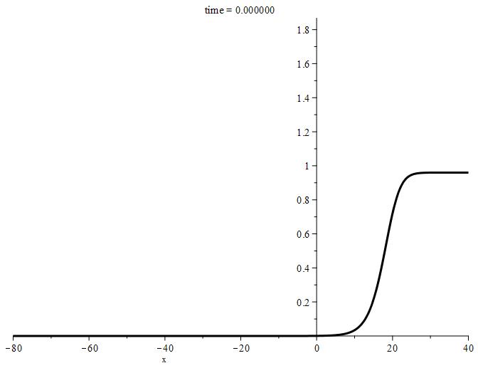
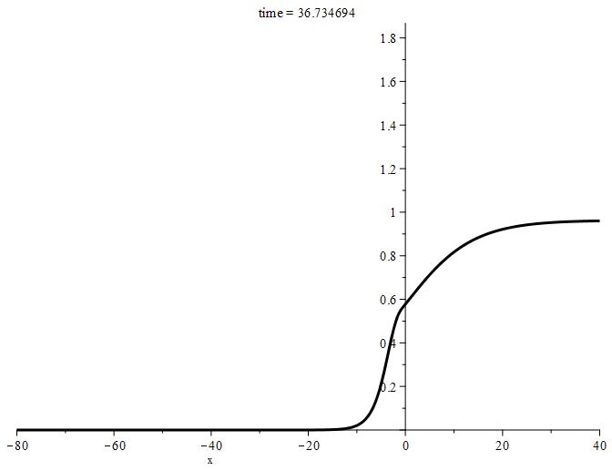
Figure 13. Left: Initial position of the shock wave $(6/25)\mathop{\mathrm{sech}}\nolimits(-4+(1/5)x)^{2}+(12/25)\tanh(-4+(1/5)x)+12/25$, $t=0$.
Right: The smooth motion breaks as the inflection point reaches the boundary of the barrier, $t=36$

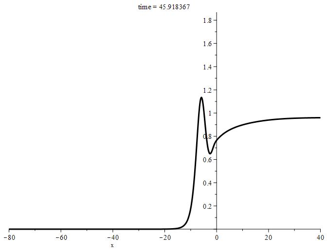
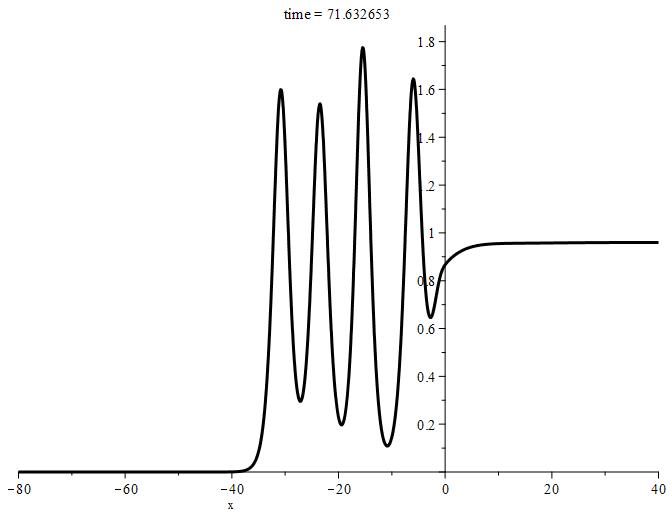
Figure 14. Left: Oscillation begins, $t=45$.
Right: and continues $t=72$

4. Conclusion and numeric considerations

The results may be of a practical use. For once, the form of the reflected wave may be used to estimate the thickness and/or the density of the viscous barrier. A refraction may also be predicted.

The figures in this paper were generated numerically using Maple PDETools package. The mode of operation uses the default Euler method, which is a centered implicit scheme, and can be used to find solutions to evolution PDEs. This implicit scheme is unconditionally stable for many problems (though this may need to be checked).

Yet note that an accurate presentation of oscillations and/or sole peaks requires the choice of the Maple procedure’s spacestep and/or the timestep parameters corresponding to a typical length and height of the solution detail.

Qualitative estimations of the refraction coefficient, based on the relative decay of the KdV selected conservation laws will be published elsewhere.

References

- [1] Stefan C. Mancas, Ronald Adams Dissipative periodic and chaotic patterns to the KdV–Burgers and Gardner equations // arXiv:1905.12626 [nlin.PS]
- [2] Samokhin A.V., Reflection and refraction of solitons by the KdV Burgers equation in nonhomogeneous dissipative media, Theoretical and Mathematical Physics, 197(1): 1527 1533 (2018) DOI: 10.1134/S0040577918100094
- [3] Samokhin A., Nonlinear waves in layered media: solutions of the KdV — Burgers equation.// Journal of Geometry and Physics 130 (2018) pp. 33 -39 https://doi.org/10.1016/j.geomphys.2018.03.016
- [4] A. Samokhin, On nonlinear superposition of the KdV-Burgers shock waves and the behavior of solitons in a layered medium.// Journal of Differential Geometry and its Applications. 54, Part A, October 2017, pp 91–99. https://doi.org/10.1016/j.difgeo.2017.03.001
- [5] R.L. Pego, P. Smereka, M.I. Weinstein. Oscillatory instability of traveling waves for a KdV-Burgers equation // Physica D. 67 (1993), p. 45–65.
- [6] A.P. Chugainova, V.A. Shargatov. Stability of non-stationary solutions of a generalized Korteweg-de Vries-Burgers equation// Comp. Math.and Math. Physics. Vol. 55(2), (2015), 253 -266. (in Russian)