An Improved Gradient Method with Approximately Optimal Stepsize Based on Conic model for Unconstrained Optimization

Abstract

A new type of stepsize, which was recently introduced by Liu and Liu (Optimization, 67(3), 427-440, 2018), is called approximately optimal stepsize and is quit efficient for gradient method. Interestingly, all gradient methods can be regarded as gradient methods with approximately optimal stepsizes. In this paper, based on the work (Numer. Algorithms 78(1), 21-39, 2018), we present an improved gradient method with approximately optimal stepsize based on conic model for unconstrained optimization. If the objective function $f$ is not close to a quadratic on the line segment between the current and latest iterates, we construct a conic model to generate approximately optimal stepsize for gradient method if the conic model can be used; otherwise, we construct some quadratic models to generate approximately optimal stepsizes for gradient method. The convergence of the proposed method is analyzed under suitable conditions. Numerical comparisons with some well-known conjugate gradient software packages such as CG$\_$DESCENT (SIAM J. Optim. 16(1), 170-192, 2005) and CGOPT (SIAM J. Optim. 23(1), 296-320, 2013) indicate the proposed method is very promising.

1 Introduction

Consider the following unconstrained optimization problem

$$\mathop{\min}\limits_{x\in{R^{n}}}f(x),$$

where $f:{R^{n}}\to R$ is continuously differentiable and its gradient is denoted by $g$.

The gradient method takes the following form

$${x_{k+1}}={x_{k}}-{\alpha_{k}}{g_{k}},$$

where ${\alpha_{k}}$ is the stepsize and $g_{k}$ is the gradient of $f$ at $x_{k}$.

Throughout this paper, $g_{k}=g(x_{k}),\;f_{k}=f(x_{k}),\;s_{k-1}=x_{k}-x_{k-1},\;y_{k-1}=g_{k}-g_{k-1}$ and $\left\|\cdot\right\|$ stands for the Euclidean norm.

It is widely accepted that the stepsize is of great importance to the numerical performance of gradient method Asmundis2013On . In 1847, Cauchy Cauchy1847M presented the steepest descent method, where the stepsize is determined by

$${\alpha_{k}^{SD}}=\arg\;\mathop{\min}\limits_{\alpha>0}f({x_{k}}-\alpha{g_{k}}).$$

The steepest descent method usually converges slowly. In 1988, Barzilai and Borwein Barzilai1988Two presented a new gradient method (BB method), where the stepsize is given by

$$\alpha_{k}^{B{B_{1}}}=\frac{\|s_{k-1}\|^{2}}{s_{k-1}^{T}y_{k-1}}\;\;\;\;\;\text{or}\;\;\;\;\;\;\alpha_{k}^{B{B_{2}}}=\frac{{s_{k-1}^{T}{y_{k-1}}}}{{\parallel{y_{k-1}}{\parallel^{2}}}}.$$

Clearly, the BB method is in essence a gradient method, but the choice of the stepsize is different from $\alpha_{k}^{SD}$.

Due to the simplicity and numerical efficiency, the BB method has enjoyed great developments during these years. The BB method has been proved to be globallyRaydan1993On and linearly convergent Dai2002Rlinear for any dimensional strictly convex quadratic functions. In 1997, Raydan Raydan1997The presented a global BB method for general nonlinear unconstrained optimization by incorporating the nonmonotone line search (GLL line search) Grippo1986A , and the numerical results in Raydan1997The suggested that the BB method is superior to some classical conjugate gradient methods. From then on, a number of modified BB stepsizes have been exploited for gradient methods. Dai et al. Dai2006CBB presented the cyclic BB method for unconstrained optimization. Using the interpolation scheme, Dai et al. Dai2002Modified presented two modified BB stepsizes for gradient methods. Based on some modified secant equations, Xiao et al. Xiao2010Notes designed four modified BB stepsizes for gradient methods. According to a fourth order model and some modified secant equations, Biglari and Solimanpur Biglari2013Scaling presented some modified gradient methods with modified BB stepsizes, and the numerical results in Biglari2013Scaling indicated that these modified BB methods are efficient. Miladinović et al. Miladinovic2011Scalar proposed a new stepsize based on the usage of both the quasi-Newton property and the Hessian inverse approximation by an appropriate scalar matrix for gradient method.

Different from the above modified BB methods, Liu and Liu Liu2018GMAOSquad introduced a new type of stepsize for gradient method in 2018, which is called approximately optimal stepsize and is quite efficient for gradient method.

Definition 1.1 Suppose that $f$ is continuously differentiable, and let ${\phi_{k}}(\alpha)$ be an approximation model of $f(x_{k}-\alpha g_{k})$, where $g_{k}=\nabla f\left(x_{k}\right)$. A positive number ${\alpha_{k}^{AOS}}$ is called the approximately optimal stepsize associated to ${\phi_{k}}(\alpha)$ for gradient method, if ${\alpha_{k}^{AOS}}$ satisfies

$${\alpha_{k}^{AOS}}=\arg\;\mathop{\min}\limits_{\alpha>0}{\phi_{k}}(\alpha).$$

The approximately optimal stepsize is generally calculated easily and can be applied to unconstrained optimization. In any gradient method for strictly convex quadratic minimization problems, the stepsize $\alpha_{k}$ can also be generated by minimizing the following quadratic approximation model:

$${\phi_{k}}\left(\alpha\right)={f_{k}}-\alpha{\left\|{{g_{k}}}\right\|^{2}}+\frac{1}{2}{\alpha^{2}}g_{k}^{T}\left({\frac{1}{{{\alpha_{k}}}}I}\right){g_{k}},$$

where ${\frac{1}{{{\alpha_{k}}}}I}$ is an approximation to the Hessian matrix of $f$ at $x_{k}$. Then, the stepsize $\alpha_{k}$ is the approximately optimal stepsizes associated to the above-mentioned ${\phi_{k}}\left(\alpha\right)$ for gradient method. As a result, all gradient methods can be regarded as gradient methods with approximately optimal stepsizes in this sense.

We see from the definition of approximately optimal stepsize that the numerical performance of gradient method with approximately optimal stepsize depends heavily on approximation model ${\phi_{k}}(\alpha)$. Some gradient methods with approximately optimal stepsizes Liu2018GMAOScone ; Liu2018Several ; Liu2018GMAOSNABB ; Liu2019TensorBB were later proposed for unconstrained optimization, and the numerical results in Liu2018GMAOScone ; Liu2018Several ; Liu2018GMAOSNABB ; Liu2019TensorBB suggested that these gradient methods with approximately optimal stepsizes are surprisingly efficient.

In those gradient methods with approximately optimal stepsizes Liu2018GMAOScone ; Liu2018Several ; Liu2018GMAOSNABB ; Liu2019TensorBB , the gradient method with approximately optimal stepsizes based on conic model Liu2018GMAOScone has enjoyed some attentions Snezana due to its good nice numerical performance. In this paper, we present an improved gradient method with approximately optimal optimal optimal stepsize based on conic model for unconstrained optimization. In the proposed method, when the objective function $f$ is not close to a quadratic function on the line segment between $x_{k-1}$ and $x_{k}$, a conic model is exploited to generate approximately optimal stepsize if the conic model can be used. Otherwise, some quadratic models are constructed to derive approximately optimal stepsizes. We analyze the convergence of the proposed method under mild conditions. Two collect sets denoted by 80pAdr and 144pCUTEr, which are from Andrei2008An and Gould2001CUTEr , respectively, are used to examine the effectiveness of the test methods. Some numerical experiments indicate that the proposed method is superior to the limited memory conjugate gradient software package CG$\_$DESCENT (6.0) HagerZhang2013The for 80pAdr and is comparable to CG$\_$DESCENT (5.0) Hager2005A for 144pCUTEr, and performs better than CGOPT Dai2013CGOPT for 80pAdr and is comparable to CGOPT for 144pCUTEr.

The remainder of this paper is organized as follows. In Section 2, we exploit some approximation models including a conic model and quadratic models to derive efficient approximately optimal stepsizes for gradient method. In Section 3, we present an improved gradient method with approximately optimal stepsize based on conic model, and analyze the global convergence of the proposed method under some suitable conditions. In Section 4, some numerical experiments are done to examine the effectiveness of the proposed method. Conclusions and discussions are given in the last section.

2 Derivation of the Approximately Optimal Stepsize

In the section, based on the properties of the objective function $f$, some approximation models including a conic model and quadratic models are exploited to generate approximately optimal stepsize for gradient method.

According to the definition of approximately optimal stepsize in Section 1, we know that the effectiveness of approximately optimal stepsize will rely on the approximation model. We determine the approximation models based on the following observations.

Define

$${\mu_{k}}=\left|{\frac{{2\left({{f_{k-1}}-{f_{k}}+g_{k}^{T}{s_{k-1}}}\right)}}{{s_{k-1}^{T}{y_{k-1}}}}-1}\right|.$$

According to Dai2002Modified ; Yuan1995A , $\mu_{k}$ is a quantity showing how $f(x)$ is close to a quadratic on the line segment between $x_{k-1}$ and $x_{k}$. If the following condition Liu2018GMAOScone ; Liu2019TensorBB holds, namely,

$${\mu_{k}}\leq{c_{1}}\;\;\;\;\text{or}\;\;\;\;\max\left\{{{\mu_{k}},{\mu_{k-1}}}\right\}\leq{c_{2}},$$

where $c_{1}$ and $c_{2}$ are small positives and $c_{1}<c_{2}$, then $f$ might be close to a quadratic on the line segment between $x_{k-1}$ and $x_{k}$. General iterative methods, which are often based on quadratic model, have been quite successful in solving practical optimization problems Han2005An , since quadratic model can approximates the objective function $f$ well at a small neighbourhood of $x_{k}$ in many cases. Consequently, if $f$ is close to a quadratic on the line segment between $x_{k-1}$ and $x_{k}$, quadratic model is preferable. However, when $x_{k}$ is far from the minimizer, quadratic model might not work very well if the objective function $f$ possesses high non-linearity Sun1996Optimization ; Sun2012A . To address the drawback, some conic models Sun2012A ; Davidon1980Conic ; Sorensen1980The have been exploited to approximate the objective function. The conic functions, which interpolate both function values and gradients at the latest two iterates, can fit exponential functions, penalty functions or other functions which share with conics the property of increasing rapidly near some $n-1$ dimensional hyperplane in $R^{n}$ Davidon1980Conic . All of these indicate that, when $f$ is not close to a quadratic function on the line segment between $x_{k-1}$ and $x_{k}$, conic models may serve better than quadratic model Sorensen1980The .

Based on the above observations, we determine approximately optimal stepsize for gradient method in the following cases.

Case I: Conic Model

When $f$ is not close to a quadratic on the line segment between $x_{k-1}$ and $x_{k}$, we consider the following conic model :

$${\phi_{k}}\left(d\right)={f_{k}}+\frac{{g_{k}^{T}d}}{{1+b_{k}^{T}d}}+\frac{{{\alpha^{2}}}}{2}\frac{{d^{T}{B_{k}}d}}{{{{\left({1+b_{k}^{T}d}\right)}^{2}}}},$$

where

$${b_{k}}=\frac{{1-{\gamma_{k}}}}{{{\gamma_{k}}g_{k-1}^{T}{s_{k-1}}}}{g_{k-1}},\;{\gamma_{k}}=\frac{{-g_{k-1}^{T}{s_{k-1}}}}{{{\rho_{k}}+{f_{k-1}}-{f_{k}}}},\;\;{\rho_{k}}=\sqrt{\Delta}_{k},\;\;\Delta_{k}{\rm{=}}{\left({{f_{k-1}}-{f_{k}}}\right)^{2}}-\left({g_{k}^{T}{s_{k-1}}}\right)\left({g_{k-1}^{T}{s_{k-1}}}\right)$$

and $B_{k}$ is generated by imposing generalized BFGS update formula Sun2012A on a positive scalar matrix $D_{k}$:

$${B_{k}}={D_{k}}-\frac{{{D_{k}}{v_{k-1}}v_{k-1}^{T}{D_{k}}}}{{v_{k-1}^{T}{D_{k}}{v_{k-1}}}}+\frac{{{r_{k-1}}r_{k-1}^{T}}}{{v_{k-1}^{T}{r_{k-1}}}},$$

where ${r_{k-1}}={\bar{y}_{k-1}}/{\gamma_{k}}$, ${v_{k-1}}={\gamma_{k}}{s_{k-1}}$ and ${\bar{y}_{k-1}}={\gamma_{k}}{g_{k}}-\dfrac{1}{{{\gamma_{k}}}}{g_{k-1}}$. Here we take the scalar matrix $D_{k}$ as $D_{k}=\xi_{1}\dfrac{{{v_{k-1}^{T}}v_{k-1}}}{{v_{k-1}^{T}{r_{k-1}}}}I$ , where $\xi_{1}\geq 1$. It is easy to verify that, if ${v_{k-1}^{T}{r_{k-1}}}>0$, then $D_{k}$ is symmetric positive definite and thus $B_{k}$ is symmetric positive definite. In order to improve the numerical performance, we restrict ${\gamma_{k}}=\max\left\{{\min\left\{{{\gamma_{k}},2}\right\},0.01}\right\}$ and the coefficient $\frac{{1-{\gamma_{k}}}}{{{\gamma_{k}}g_{k-1}^{T}{s_{k-1}}}}$ of $b_{k}$ as $\max\left\{{\min\left\{{{\frac{{1-{\gamma_{k}}}}{{{\gamma_{k}}g_{k-1}^{T}{s_{k-1}}}}},5000}\right\},-5000}\right\}$.

By substituting $d=-\alpha g_{k}$ into the above conic model $\phi_{k}\left(d\right)$, we obtain that

$$\phi_{k}^{1}\left({\alpha}\right)=f\left({{x_{k}}}\right)-\frac{{\alpha g_{k}^{T}{g_{k}}}}{{1-\alpha b_{k}^{T}{g_{k}}}}+\frac{{{\alpha^{2}}}}{2}\frac{{g_{k}^{T}{B_{k}}{g_{k}}}}{{{{\left({1-\alpha b_{k}^{T}{g_{k}}}\right)}^{2}}}}.$$

It is clear that $\alpha_{k}=\frac{1}{b^{T}_{k}g_{k}}$ is the singular point of $\phi_{k}^{1}\left(\alpha\right)$, ${\phi_{k}^{1}}^{\prime}\left(\alpha\right)=\frac{{\alpha\left({g_{k}^{T}{B_{k}}{g_{k}}+g_{k}^{T}{g_{k}}b_{k}^{T}{g_{k}}}\right)-g_{k}^{T}{g_{k}}}}{{{{\left({1-\alpha b_{k}^{T}{g_{k}}}\right)}^{3}}}}$ and $\phi_{k}^{1}\left(\alpha\right)$ is continuous differentiable in $R\backslash\left\{{1/b_{k}^{T}{g_{k}}}\right\}$.

If $\Delta_{k}>0$, ${v_{k-1}^{T}{r_{k-1}}}>0$ and ${g_{k}^{T}{B_{k}}{g_{k}}+\left({g_{k}^{T}{g_{k}}}\right)\left({b_{k}^{T}{g_{k}}}\right)}\neq 0$, by imposing $\dfrac{{d\phi_{k}^{1}}}{{d\alpha}}{\rm{=}}0$ we obtain the unique stationary point of $\phi_{k}^{1}\left(\alpha\right)$:

$$\alpha^{S}_{k}=\frac{{g_{k}^{T}{g_{k}}}}{{g_{k}^{T}{B_{k}}{g_{k}}+\left({g_{k}^{T}{g_{k}}}\right)\left({b_{k}^{T}{g_{k}}}\right)}}.$$

We analyze the properties of the stationary point $\alpha_{k}^{S}$ in the following two cases.

(1) The singular point $\alpha_{k}=\dfrac{1}{b_{k}^{T}g_{k}}<0$. If ${g_{k}^{T}{B_{k}}{g_{k}}+\left({g_{k}^{T}{g_{k}}}\right)\left({b_{k}^{T}{g_{k}}}\right)}<0$, then we know $\alpha^{S}_{k}<\frac{1}{b_{k}^{T}g_{k}}$. By $\phi_{k}^{1}\left(\alpha\right)$, it is not difficult to obtain that

$$\mathop{\lim}\limits_{\alpha\to 1/b_{k}^{T}{g_{k}}}{\phi_{1}}\left(\alpha\right){\rm{=+}}\infty\;\;\;{\rm{and}}\;\;\;\;\mathop{\lim}\limits_{\alpha\to{\rm{+}}\infty}{\phi_{1}}\left(\alpha\right){\rm{=}}{f_{k}}+\frac{{g_{k}^{T}{g_{k}}}}{{b_{k}^{T}{g_{k}}}}+\frac{{g_{k}^{T}{B_{k}}{g_{k}}}}{{2{{\left({b_{k}^{T}{g_{k}}}\right)}^{2}}}}\;$$

and ${\phi_{k}^{1}}^{\prime}\left(\alpha\right)<0$ for $\alpha>\frac{1}{b_{k}^{T}g_{k}}$. Therefore, there no exists $\alpha^{*}>0$ such that $\alpha^{*}=\mathop{\min}\limits_{\alpha>0}\;{\phi_{k}^{1}}\left(\alpha\right)$. Consequently, if ${g_{k}^{T}{B_{k}}{g_{k}}+\left({g_{k}^{T}{g_{k}}}\right)\left({b_{k}^{T}{g_{k}}}\right)}\leq 0$, then we will switch to Case II. Here we only consider the case of ${g_{k}^{T}{B_{k}}{g_{k}}+\left({g_{k}^{T}{g_{k}}}\right)\left({b_{k}^{T}{g_{k}}}\right)}>0$. In the case we know that $\alpha_{k}^{S}>0$. If $\alpha>\alpha_{k}^{S}$, then ${\alpha\left({g_{k}^{T}{B_{k}}{g_{k}}+g_{k}^{T}{g_{k}}b_{k}^{T}{g_{k}}}\right)-g_{k}^{T}{g_{k}}}>0$, which together with ${1-\alpha b_{k}^{T}{g_{k}}}>0$ implies that

$${\phi_{1}}^{\prime}\left(\alpha\right)>0$$

for $\alpha>\alpha_{k}^{S}$. By ${\phi_{1}}^{\prime}\left(0\right)=-\left\|g_{k}\right\|^{2}<0$, the continuous differentiability of $\phi_{k}^{1}\left(\alpha\right)$ in $R\backslash\left\{{1/b_{k}^{T}{g_{k}}}\right\}$, the uniqueness of the stationary point and ${\phi_{1}}^{\prime}\left(\alpha^{S}_{k}\right)=0$, we know that ${\phi_{1}}^{\prime}\left(\alpha\right)<0$ holds for $\alpha\in\left[0,\alpha_{k}^{S}\right)$. Therefore, the stationary point $\alpha^{S}_{k}$ satisfies

$${\alpha^{S}_{k}}=\mathop{\min}\limits_{\alpha>0}\;{\phi_{1}}\left(\alpha\right),$$

which means that the stationary point $\alpha^{S}_{k}$ is the approximately optimal stepsize associated to $\phi_{k}^{1}\left(\alpha\right)$.

(2)The singular point $\alpha_{k}=\frac{1}{b_{k}^{T}g_{k}}>0$. It is obvious that the stationary point $\alpha^{S}_{k}$ satisfies $0<{\alpha^{S}_{k}}<\frac{1}{{b_{k}^{T}{g_{k}}}}$. If $\alpha^{S}_{k}<\alpha<\frac{1}{b^{T}_{k}g_{k}}$, we obtain that $1-\alpha b^{T}_{k}g_{k}>0$ and ${\alpha\left({g_{k}^{T}{B_{k}}{g_{k}}+g_{k}^{T}{g_{k}}b_{k}^{T}{g_{k}}}\right)-g_{k}^{T}{g_{k}}}>0$, which imply that

$${\phi_{1}}^{\prime}\left(\alpha\right)>0$$

for $\alpha\in\left(\alpha^{S}_{k},\frac{1}{b^{T}_{k}g_{k}}\right)$. By ${\phi_{1}}^{\prime}\left(0\right)=-\left\|g_{k}\right\|^{2}<0$, ${\phi_{1}}^{\prime}\left(\alpha^{S}_{k}\right)=0$, the continuous differentiability of $\phi_{k}^{1}\left(\alpha\right)$ in $R\backslash\left\{{1/b_{k}^{T}{g_{k}}}\right\}$ and the uniqueness of the stationary point, we know that ${\phi_{1}}^{\prime}\left(\alpha\right)<0$ holds for $\alpha\in\left[0,\alpha^{S}_{k}\right)$. Therefore, the stationary point $\alpha^{S}_{k}$ is a local minimizer of $\phi_{k}^{1}\left(\alpha\right)$ and

$$\;{\phi_{1}}\left({\alpha_{k}^{S}}\right)={f_{k}}-\frac{{{{\left({g_{k}^{T}{g_{k}}}\right)}^{2}}}}{{2g_{k}^{T}{B_{k}}{g_{k}}}}.$$

If $\alpha>\frac{1}{b_{k}^{T}g_{k}}$, then we have $1-\alpha b_{k}^{T}g_{k}<0$,

$$\mathop{\lim}\limits_{\alpha\to{{\left({1/b_{k}^{T}{g_{k}}}\right)}^{+}}}{\phi_{1}}\left(\alpha\right){\rm{=+}}\infty\;\;\;\;\;{\rm{and}}\;\;\;\;\mathop{\lim}\limits_{\alpha\to{\rm{+}}\infty}{\phi_{1}}\left(\alpha\right){\rm{=}}{f_{k}}+\frac{{g_{k}^{T}{g_{k}}}}{{b_{k}^{T}{g_{k}}}}+\frac{{g_{k}^{T}{B_{k}}{g_{k}}}}{{2{{\left({b_{k}^{T}{g_{k}}}\right)}^{2}}}},\;$$

which together with the fact that ${\phi_{1}}^{\prime}\left(\alpha\right)<0$ holds for $\alpha>\frac{1}{b_{k}^{T}g_{k}}$ implies that

$${\phi_{1}}\left({\alpha_{k}^{S}}\right)-\mathop{\lim}\limits_{\alpha\to{\rm{+}}\infty}{\phi_{1}}\left(\alpha\right)={\phi_{1}}\left({\alpha_{k}^{S}}\right)-{f_{k}}-\frac{{g_{k}^{T}{g_{k}}}}{{b_{k}^{T}{g_{k}}}}-\frac{{g_{k}^{T}{B_{k}}{g_{k}}}}{{2{{\left({b_{k}^{T}{g_{k}}}\right)}^{2}}}}=-\frac{{{{\left({g_{k}^{T}{g_{k}}}\right)}^{2}}}}{{2g_{k}^{T}{B_{k}}{g_{k}}}}-\frac{{g_{k}^{T}{g_{k}}}}{{b_{k}^{T}{g_{k}}}}-\frac{{g_{k}^{T}{B_{k}}{g_{k}}}}{{2{{\left({b_{k}^{T}{g_{k}}}\right)}^{2}}}}<0$$

holds for $\alpha>\frac{1}{b_{k}^{T}g_{k}}$. Therefore, the stationary point $\alpha^{S}_{k}$ satisfies

$${\alpha^{S}_{k}}=\arg\;\mathop{\min}\limits_{\alpha>0}{\phi_{k}^{1}}(\alpha),$$

which implies that the stationary point $\alpha^{S}_{k}$ is the approximately optimal stepsize associated to $\phi_{k}^{1}\left(\alpha\right)$.

It is observed by numerical experiments that the bound $\left[\alpha_{k}^{B{B_{2}}},\alpha_{k}^{B{B_{1}}}\right]$ for $\alpha^{S}_{k}$ is very preferable for the case of $s_{k-1}^{T}y_{k-1}>0$. Therefore, if the condition (2.1) does not hold and the conditions

$$\Delta_{k}>0,\;\;{v_{k-1}^{T}{r_{k-1}}}>0\;\;\text{and }\;\;{g_{k}^{T}{B_{k}}{g_{k}}+\left({g_{k}^{T}{g_{k}}}\right)\left({b_{k}^{T}{g_{k}}}\right)}>0$$

hold, the approximately optimal stepsize is taken as follows:

$$\alpha_{k}^{AOS\;(1)}=\left\{{\begin{array}[]{*{20}{c}}{\max\left\{{\min\left\{{\alpha_{k}^{S},\alpha_{k}^{B{B_{1}}}}\right\},\alpha_{k}^{B{B_{2}}}}\right\},\;\;\;{\rm{if}}\;s_{k-1}^{T}{y_{k-1}}>0,}\\ {\alpha_{k}^{S},\;\;\;\;\;\;\;\;\;\;\;\;\;\;\;\;\;\;\;\;\;\;\;\;\;\;\;\;\;\;\;\;\;\;\;\;\;\;\;\;\;\;\;\;\;\;\;\;\;{\rm{if}}\;s_{k-1}^{T}{y_{k-1}}\leq 0.}\end{array}}\right.$$

Case II: Quadratic Models

(i)$s_{k-1}^{T}y_{k-1}>0$

It is generally accepted that quadratic model will serve well if $f$ is close to a quadratic function on the segment between $x_{k-1}$ and $x_{k}$. So we do not wish to abandon quadratic model because of the large amount of practical experience and theoretical work indicating its suitability. If the condition (2.1) holds and $s_{k-1}^{T}y_{k-1}>0$, or the conditions (2.2) do not hold and $s_{k-1}^{T}y_{k-1}>0$, we consider the following quadratic approximation model:

$$\phi_{k}^{2}(\alpha)=f({x_{k}})-\alpha\parallel{g_{k}}{\parallel^{2}}+\frac{1}{2}{\alpha^{2}}g_{k}^{T}{B_{k}}{g_{k}},$$

where $B_{k}$ is a symmetric and positive definite approximation to the Hessian matrix. Taking into account the storage cost and computational cost, $B_{k}$ is generated by imposing the quasi-Newton update formula on a scalar matrix. Taking the scalar matrix as $D_{k}=\xi_{2}\frac{{y_{k-1}^{T}{y_{k-1}}}}{{s_{k-1}^{T}{y_{k-1}}}}I$, where $\xi_{2}\geq 1$, and imposing the modified BFGS update formula Zhang1999NewBFGS on the scalar matrix $D_{k}$, we obtain

$${B_{k}}={D_{k}}-\frac{{{D_{k}}{s_{k-1}}s_{k-1}^{T}{D_{k}}}}{{s_{k-1}^{T}{D_{k}}{s_{k-1}}}}{\rm{+}}\frac{{{\bar{y}_{k-1}}^{T}{\bar{y}_{k-1}}}}{{s_{k-1}^{T}{\bar{y}_{k-1}}}},$$

where ${\bar{y}_{k-1}}={y_{k-1}}+\frac{{\bar{r}_{k}}}{\left\|{{s_{k-1}}}\right\|^{2}}s_{k-1}$ and ${\bar{r}_{k}}={3{{\left({{g_{k}}+{g_{k-1}}}\right)}^{T}}{s_{k-1}}+6({f_{k-1}}-{f_{k}})}$.

Since there exists $u_{1}\in\left[{0,1}\right]$ such that

$$\bar{r}_{k}=3\left({s_{k-1}^{T}{y_{k-1}}-s_{k-1}^{T}{\nabla^{2}}f({x_{k-1}}+{u_{1}}{s_{k-1}}){s_{k-1}}}\right),$$

in order to improve the numerical performance we restrict ${\bar{r}_{k}}$ as

$$\bar{r}_{k}=\min\left\{{\max\left\{{\bar{r}_{k},-{\bar{\eta}}s_{k-1}^{T}{y_{k-1}}}\right\},{\bar{\eta}}s_{k-1}^{T}{y_{k-1}}}\right\},$$

where $0<\bar{\eta}<0.1$.

It follows from (2.5) that ${s_{k-1}^{T}{\bar{y}_{k-1}}}=s_{k-1}^{T}y_{k-1}+\bar{r}_{k}\geq(1-\bar{\eta})s_{k-1}^{T}y_{k-1}$ when $s_{k-1}^{T}y_{k-1}>0$, which implies the following lemma.

Lemma 2.1 Suppose that $s_{k-1}^{T}y_{k-1}>0$. Then ${s_{k-1}^{T}{\bar{y}_{k-1}}}>0$ and $B_{k}$ is symmetric and positive definite.

Imposing $\frac{{d{\phi_{k}^{2}}}}{{d\alpha}}=0$, we obtain

$$\bar{\alpha}_{k}^{AOS(2)}=\frac{{g_{k}^{T}{g_{k}}}}{{g_{k}^{T}{B_{k}}{g_{k}}}}=\frac{{g_{k}^{T}{g_{k}}}}{{\frac{{{\xi_{2}}{{\left\|{{y_{k-1}}}\right\|}^{2}}}}{{s_{k-1}^{T}{y_{k-1}}}}\left({{{\left\|{{g_{k}}}\right\|}^{2}}-\frac{{{{\left({g_{k}^{T}{s_{k-1}}}\right)}^{2}}}}{{{{\left\|{{s_{k-1}}}\right\|}^{2}}}}}\right)+{{\left({\frac{{g_{k}^{T}{y_{k-1}}}}{{{{\left({s_{k-1}^{T}{{\bar{y}}_{k-1}}}\right)}^{2}}}}+\frac{{{{\bar{r}}_{k}}g_{k}^{T}{s_{k-1}}}}{{{{\left({s_{k-1}^{T}{{\bar{y}}_{k-1}}}\right)}^{2}}{{\left\|{{s_{k-1}}}\right\|}^{2}}}}}\right)}^{2}}}}.$$

By $s_{k-1}^{T}y_{k-1}>0$ and Lemma 2.1, we know that $\bar{\alpha}_{k}^{AOS(2)}$ is the approximately optimal stepsize associated to $\phi_{k}^{2}(\alpha)$.

It is also observed by numerical experiments that the bound $\left[\alpha_{k}^{B{B_{2}}},\alpha_{k}^{B{B_{1}}}\right]$ for $\alpha_{k}$ in (2.6) is very preferable. Therefore, if the condition (2.1) holds and $s_{k-1}^{T}{y_{k-1}}>0$, or the conditions (2.3) do not hold and $s_{k-1}^{T}{y_{k-1}}>0$, the approximately optimal stepsize is taken as the truncation form of $\bar{\alpha}_{k}^{AOS(2)}$ :

$$\alpha_{k}^{AOS\;(2)}=\max\left\{{\min\left\{{\bar{\alpha}_{k}^{AOS(2)},\alpha_{k}^{B{B_{1}}}}\right\},\alpha_{k}^{B{B_{2}}}}\right\}.$$

(ii)$s_{k-1}^{T}y_{k-1}\leq 0$

It is a challenging task to determine a suitable stepsize for gradient method when $s_{k-1}^{T}y_{k-1}\leq 0.$ In some modified BB methods Dai2002Modified ; Xiao2010Notes , the stepsize is set simply to ${\alpha_{k}}=10^{30}$ for the case of $s_{k-1}^{T}y_{k-1}\leq 0$. It is too simple to consume expensive computational cost for searching a suitable stepsize for gradient method.

In Liu2018GMAOSNABB , Liu et al. proposed a simple and efficient strategy for choosing the stepsize for the case of $s_{k-1}^{T}y_{k-1}\leq 0$: $\alpha_{k}=\delta\alpha_{k-1}$, where $\delta>0$. Liu and Liu Liu2018Several designed an approximation model to generate approximately optimal stepsize. Liu and Liu Liu2018GMAOScone designed two approximation models to generate two approximately optimal stepsizes, and the numerical results in Liu2018GMAOScone showed that these approximately optimal stepsize are efficient. We take the stepsize Liu2018GMAOScone for gradient method, which is described here for completeness.

If the condition (2.1) holds and $s_{k-1}^{T}y_{k-1}\leq 0$, or the conditions (2.3) do not hold and $s_{k-1}^{T}y_{k-1}\leq 0$, we design other approximation models to derive approximately optimal stepsizes. Suppose for the moment that $f$ is twice continuously differentiable, the second order Taylor expansion is

$$f({x_{k}}-\alpha{g_{k}})=f({x_{k}})-\alpha g_{k}^{T}{g_{k}}+\frac{1}{2}{\alpha^{2}}g_{k}^{T}{\nabla^{2}}f({x_{k}}){g_{k}}+o({\alpha^{2}}).$$

For a very small $\tau_{k}>0$, we have that

$${\nabla^{2}}f({x_{k}}){g_{k}}\approx-\frac{{g({x_{k}}-\tau_{k}{g_{k}})-g({x_{k}})}}{\tau_{k}},\;$$

which gives a new approximation model

$$\phi_{k}^{3}\left(\alpha\right)=f({x_{k}})-\alpha g_{k}^{T}{g_{k}}+\frac{1}{2}{\alpha^{2}}|g_{k}^{T}(g({x_{k}}-\tau_{k}{g_{k}})-g({x_{k}}))/{\tau_{k}}|.$$

If ${g_{k}^{T}(g({x_{k}}-\tau_{k}{g_{k}})-g({x_{k}}))/{\tau_{k}}}\neq 0$, then by imposing $\dfrac{{d\phi_{k}^{3}}}{{d\alpha}}=0$ and the coefficient of $\alpha^{2}$ in $\phi_{k}^{3}\left(\alpha\right)$, we obtain the approximately optimal stepsize associated to $\phi_{k}^{3}\left(\alpha\right)$:

$$\alpha^{AOS(3)}_{k}=\frac{{g_{k}^{T}{g_{k}}}}{|{g_{k}^{T}(g({x_{k}}-\tau_{k}{g_{k}})-g({x_{k}}))/{\tau_{k}}|}}.$$

When ${g_{k}^{T}(g({x_{k}}-\tau_{k}{g_{k}})-g({x_{k}}))/{\tau_{k}}}=0$, similar to Liu2018GMAOSNABB , the stepsize $\alpha_{k}$ $\alpha_{k}$ is computed by

$$\alpha_{k}=\delta\alpha_{k-1},$$

where $\delta>0$.

To obtain the stepsize $\alpha_{k}$ in (2.8), it has the cost of an extra gradient evaluation, which may result in great computational cost if the gradient evaluation is evoked frequently. To reduce the computational cost, we turn to consider $g_{k-1}.$ Since

$$s_{k-1}^{T}{y_{k-1}}=-{\alpha_{k-1}}g_{k-1}^{T}({g_{k}}-{g_{k-1}})={\alpha_{k-1}}(\parallel{g_{k-1}}{\parallel^{2}}-g_{k-1}^{T}{g_{k}})\leq 0,$$

we have that

$$\parallel{g_{k-1}}{\parallel^{2}}\leq g_{k-1}^{T}{g_{k}},$$

which implies

$$\frac{{\parallel{g_{k-1}}\parallel}}{{\parallel{g_{k}}\parallel}}\leq 1.$$

If $\dfrac{{\parallel{g_{k-1}}{\parallel^{2}}}}{{\parallel{g_{k}}{\parallel^{2}}}}\geq\xi_{3}$, where $\xi_{3}>0$ is close to 1, we know that $g_{k}$ and $g_{k-1}$ will incline to be collinear and $\parallel g_{k}\parallel$ and $\parallel g_{k-1}\parallel$ are approximately equal. In the case, we use $g_{k-1}^{T}{\nabla^{2}}f({x_{k}}){g_{k-1}}$ to approximate $g_{k}^{T}{\nabla^{2}}f({x_{k}}){g_{k}}$, and then use $\frac{{\left|{{{\left({(g({x_{k}}+{\alpha_{k-1}}{g_{k-1}})-g({x_{k}})}\right)}^{T}}{g_{k-1}}}\right|}}{{{\alpha_{k-1}}}}=\frac{{\left|{s_{k-1}^{T}{y_{k-1}}}\right|}}{{\alpha_{k-1}^{2}}}$ to estimate $g_{k-1}^{T}{\nabla^{2}}f({x_{k}}){g_{k-1}}$, which imply a new approximation model:

$${\phi_{k}^{4}}\left(\alpha\right)=f({x_{k}})-\alpha\parallel{g_{k}}{\parallel^{2}}+\frac{1}{2}{\alpha^{2}}\frac{{\left|{s_{k-1}^{T}{y_{k-1}}}\right|}}{{\alpha_{k-1}^{2}}}.$$

If $s_{k-1}^{T}y_{k-1}\neq 0$, by imposing $\frac{{d{\phi_{k}^{4}}}}{{d\alpha}}=0$ and the coefficient of $\alpha^{2}$ in $\phi_{k}^{4}\left(\alpha\right)$, we also obtain the approximately optimal stepsize associated to $\phi_{k}^{4}\left(\alpha\right)$:

$$\alpha^{AOS(4)}_{k}=\frac{{\parallel{g_{k}}{\parallel^{2}}}}{|{s_{k-1}^{T}{y_{k-1}}}|}{\alpha_{k-1}^{2}}.$$

As for the case of $s_{k-1}^{T}y_{k-1}=0$, the stepsize is also computed by (2.9).

Therefore, if the condition (2.1) holds and $s_{k-1}^{T}y_{k-1}\leq 0$, or the conditions (2.3) do not hold and $s_{k-1}^{T}y_{k-1}\leq 0$, the stepsize is determined by

$${\alpha_{k}}=\left\{{\begin{array}[]{*{20}{c}}{\dfrac{{g_{k}^{T}{g_{k}}}}{{|g_{k}^{T}(g({x_{k}}-{\tau_{k}}{g_{k}})-g({x_{k}}))/{\tau_{k}}|}}\;,\;\;\;\;\text{if}\;\;\dfrac{{\parallel{g_{k}}{\parallel^{2}}}}{{\parallel{g_{k-1}}{\parallel^{2}}}}<{\xi_{3}}\;\;\text{and}\;\;g_{k}^{T}(g({x_{k}}-{\tau_{k}}{g_{k}})-g({x_{k}}))/{\tau_{k}}\neq 0,}\\ {\dfrac{{\parallel{g_{k}}{\parallel^{2}}}}{{|s_{k-1}^{T}{y_{k-1}}|}}\alpha_{k-1}^{2},\;\;\;\;\;\;\;\;\;\;\;\;\;\;\;\;\;\;\;\;\;\;\;\;\;\;\;\;\;\text{if}\;\;\dfrac{{\parallel{g_{k}}{\parallel^{2}}}}{{\parallel{g_{k-1}}{\parallel^{2}}}}\geq{\xi_{3}}\;\;\;\;\;\text{and}\;\;\;\;s_{k-1}^{T}{y_{k-1}}\neq 0,}\\ {\delta{\alpha_{k-1}},\;\;\;\;\;\;\;\;\;\;\;\;\;\;\;\;\;\;\;\;\;\;\;\;\;\;\;\;\;\;\;\;\;\;\;\;\;\;\;\;\;\;\;\begin{array}[]{*{20}{c}}{\text{otherwise},}&{}\hfil&{}\hfil\end{array}}\end{array}}\right.$$

where $\delta>0$.

3 Gradient Method with Approximately Optimal Stepsize Based on Conic Model

In the section, we present an improved gradient method with approximately optimal stepsize based on conic model (we call it GM$\_$AOS (cone) for short) for unconstrained optimization. Though GLL line search Grippo1986A was firstly incorporated into the BB method Raydan1997The , it is observed by numerical experiments that for modified BB methods the nonmonotone line search (Zhang-Hager line search) proposed by Zhang and Hager Zhang2004A is preferable. Usually, the strategy (3.2) for a nonmonotone line search Birgin2000Nonmonotone is used to accelerate the convergence rate. Therefore, we adopt Zhang-Hager line search with the strategy (3.2) in GM$\_$AOS (cone). Motivated by SMCG$\_$BB LiuSMCGBB , at the first iteration we choose the initial stepsize $\alpha_{0}^{0}$ as

$$\alpha_{0}^{0}=\left\{{\begin{array}[]{*{20}{c}}{\begin{array}[]{*{20}{c}}{1,}&{\;\;\;\;\;\;\;\;\;\;\;\;\;\;\;\;\;\;\;\;\;\;\;\;\;\;\;\;\;\;\;\;\;\;\;\;\;\;\;\;\;\;\;\;\;\;\;\;\;\;\;\;\;\;\;\;\;{\rm{if}}\left|f\right|\leq{{10}^{-30}}\;{\rm{and}}\;\;{{\left\|{{x_{0}}}\right\|}_{\infty}}\leq{{10}^{-30}},}\end{array}}\\ {\begin{array}[]{*{20}{c}}{\begin{array}[]{*{20}{c}}{\begin{array}[]{*{20}{c}}{2\left|f\right|/\left\|{{g_{0}}}\right\|,}&{\;\;\;\;\;\;\;\;\;\;\;\;\;\;\;\;\;\;\;\;\;\;\;\;\;\;\;\;\;\;\;\;\;\;\;\;\;\;\;\;\;\;{\rm{if}}\left|f\right|>{{10}^{-30}}\;{\rm{and}}\;\;{{\left\|{{x_{0}}}\right\|}_{\infty}}\leq{{10}^{-30}},}\end{array}}\\ {\begin{array}[]{*{20}{c}}{\min\left\{{1,{{\left\|{{x_{0}}}\right\|}_{\infty}}/{{\left\|{{g_{0}}}\right\|}_{\infty}}}\right\},}&{\;\;\;\;\;\;\;\;\;\;\;\;\;\;\;\;\;\;\;\;\;\;{\rm{if}}\;{{\left\|{{g_{0}}}\right\|}_{\infty}}<{{10}^{7}}\;{\rm{and}}\;\;{{\left\|{{x_{0}}}\right\|}_{\infty}}>{{10}^{-30}},}\end{array}}\end{array}}\\ {\begin{array}[]{*{20}{c}}{\min\left\{{1,\max\left\{{1,{{\left\|{{x_{0}}}\right\|}_{\infty}}}\right\}/{{\left\|{{g_{0}}}\right\|}_{\infty}}}\right\},}&{{\rm{if}}\;{{\left\|{{g_{0}}}\right\|}_{\infty}}\geq{{10}^{7}}\;{\rm{and}}\;\;{{\left\|{{x_{0}}}\right\|}_{\infty}}>{{10}^{-30}}.}\end{array}}\end{array}}\end{array}}\right.$$

Now we describe GM$\_$AOS (cone) in detail.

Algorithm 1 GM$\_$AOS (cone)
Step 0 Initialization.Given a starting point ${x_{0}}\in{R^{n}}$, constants $\;\varepsilon>0,\;\lambda_{\min},\lambda_{\max},\;\eta_{\min},\;\eta_{\max},\;\sigma,\;\delta,\;\xi_{1},\;\xi_{2},\;\xi_{3},\;$

${\bar{\eta}},\;c_{1}$ and $c_{2}$. Set ${Q_{0}}=1,\;{C_{0}}={f_{0}}$ and $k:=0.$
Step 1 If $||{g_{k}}||_{\infty}\leq\varepsilon$, then stop.
Step 2 Compute the initial stepsize for Zhang-Hager line search.

Step 2.1 If $k=0$ , then compute $\alpha_{0}^{0}$ by (3.1) and set $\alpha=\alpha_{0}^{0}$, go to Step 3.

Step 2.2 If the condition (2.1) does not hold and the conditions (2.3) hold, then compute $\alpha_{k}$ by (2.4). Set

$\alpha_{k}^{0}=\max\left\{{\min\left\{{{\alpha_{k}},{\lambda_{\max}}}\right\},{\lambda_{\min}}}\right\}$ and $\alpha=\alpha_{k}^{0},$ and go to Step 3.

Step 2.3 If $s_{k-1}^{T}{y_{k-1}}>0$, then compute $\alpha_{k}$ by (2.7); otherwise compute $\alpha_{k}$ by (2.11). Set

$\alpha_{k}^{0}=\max\left\{{\min\left\{{{\alpha_{k}},{\lambda_{\max}}}\right\},{\lambda_{\min}}}\right\}$ and $\alpha=\alpha_{k}^{0},$ and go to Step 3.
Step 3 Zhang-Hager line search. If

$$f({x_{k}}-\alpha{g_{k}})\leq{C_{k}}-\sigma\alpha\parallel{g_{k}}{\parallel^{2}},\;\;$$

then go to Step 4. Otherwise, update $\alpha$ by Birgin2000Nonmonotone

$$\alpha=\left\{{\begin{array}[]{*{20}{c}}{\bar{\alpha},\;\;\;\;\;\;\;\text{if}\;\alpha>0.1\alpha_{k}^{0}\;\text{and}\;\bar{\alpha}\in[0.1\alpha_{k}^{0},0.9\alpha],}\\ {0.5\alpha,\;\;\;\text{otherwise},}\end{array}}\right.$$

where $\bar{\alpha}$ is the trial stepsize obtained by a quadratic interpolation at ${x_{k}}$ and ${x_{k}}-\alpha{g_{k}}$, go to Step 3.
Step 4 Choose $\eta_{k}\in[\eta_{\min},\eta_{\max}]$ and update $Q_{k+1},C_{k+1}$ by the following ways:

$$Q_{k+1}=\eta_{k}Q_{k}+1,C_{k+1}=(\eta_{k}Q_{k}C_{k}+f(x_{k+1}))/Q_{k+1}.$$

Step 5 Set ${\alpha_{k}}=\alpha$, ${x_{k+1}}={x_{k}}-{\alpha_{k}}{g_{k}}$, $k:=k+1$ and go to Step 1.

In what follows, we analyze the convergence and the convergence rate of GM$\_$AOS (cone). Our convergence result utilizes the following assumptions :
A1. $f$ is continuously differentiable on $R^{n}$.
A2. $f$ is bounded below on $R^{n}$.
A3. The gradient $g$ is Lipschitz continuous on $R^{n}$, namely, there exists $L>0$ such that

$$\parallel g(x)-g(y)\parallel\leq L\parallel x-y\parallel,\;\;\forall x,y\in{R^{n}}.$$

Since $d_{k}=-g_{k}$, we have $\|d_{k}\|=\|g_{k}\|$ and $g_{k}^{T}d_{k}=-\|g_{k}\|^{2}$. Therefore, by Theorem 2.2 of Zhang2004A we can easily obtain the following theorem which shows that GM$\_$AOS (cone) is globally convergent.

Theorem 3.1 Suppose that assumption A1, A2 and A3 hold. Let $\{{x_{k}}\}$ be the sequence generated by GM$\_$AOS (cone). Then

$$\liminf_{k\to\infty}\left\|g_{k}\right\|=0.$$

Furthermore, if $\eta_{\max}<1,$ then

$$\mathop{\lim}\limits_{k\to\infty}\left\|g_{k}\right\|=0.$$

Hence, every convergent subsequence of the $\{{x_{k}}\}$ approaches a stationary point $x^{\ast}$ .

Similar to the above theorem, by Theorem 3.1 of Zhang2004A , we also obtain the following theorem which implies the R-linear convergence of GM$\_$AOS (cone).

Theorem 3.2 Suppose that A1 and A3 hold, $f$ is strongly convex with unique minimizer $x^{\ast}$ and $\eta_{\max}<1$. Then there exists $\zeta\in(0,1)$ such that

$$f({x_{k}})-f({x^{*}})\leq{\varsigma^{k}}\left({f({x_{0}})-f({x^{*}})}\right),$$

for each $k\geq 0$.

4 Numerical Experiments

In the section, some numerical experiments are conducted to check the numerical performance of GM$\_$AOS (cone). Two groups of collect sets are used, and their names are described in Table 1 and Table 2, respectively. The first group of collect sets denoted by 80pAndr includes 80 test functions mainly from Andrei2008An , and their expressions and Fortran codes can be found in Andrei’s website: http://camo.ici.ro/neculai/AHYBRIDM. The dimension of each test function in 80pro$\_$Andrei is set to 10000 and the initial points are default. The second group of collect sets denoted by 144pCUTEr includes 145 test functions from CUTEr library Gould2001CUTEr , which can be found in http://users.clas.ufl.edu/hager/papers/CG/results6.0.txt. It is noted that the 144 test functions from CUTEr library Gould2001CUTEr are indeed used to test, as the default initial point is the optimal point in the test function “FLETCBV2”, so the second group of collect sets is denoted by 144pCUTEr. And the initial points and dimensions of the test functions from 144pCUTEr are default.

The BB method, the SBB4 method Biglari2013Scaling , CGOPT Dai2013CGOPT and CG$\_$DESCENTHager2005A are chosen to be compared with GM$\_$AOS (cone). All test methods are implemented by C language. The C code of GM$\_$AOS (cone) and some numerical results can be downloaded from the website: http://web.xidian.edu.cn/xdliuhongwei/en/paper.html. The codes of CGOPT and CG$\_$DESCENT can be downloaded from http://coa.amss.ac.cn/wordpress/?page_id=21 and http://users.clas.ufl.edu/hager/papers/Software, respectively.

In the numerical experiments, GM$\_$AOS (cone) uses the following parameters: $\varepsilon={10^{-6}},\;\delta=10,\;\sigma={10^{-4}},\;{\lambda_{\min}}={10^{-30}},\;{\lambda_{\max}}={10^{30}},\;\eta_{k}=1$, $\;\bar{\eta}=5.0/3\times 10^{-5}$, $\;\tau_{k}=\min\{0.1\alpha_{k-1},0.01\}$, $\xi_{1}=2.15,\;\xi_{2}=1.07,\;\xi_{3}=0.9,\;c_{1}=10^{-8}\;$ and $c_{2}=0.07$. The BB method and the SBB4 method adopt the same line search as GM$\_$AOS (cone). All the gradient methods are stopped if $\parallel{g_{k}}{\parallel_{\infty}}\leq{10^{-6}}$ is satisfied, the number of iterations exceeds $140000$, or the number of function evaluations exceeds $50000$. CG$\_$DESCENT and CGOPT are terminated if $\parallel{g_{k}}{\parallel_{\infty}}\leq{10^{-6}}$ is satisfied or the number of iterations exceeds $140000$, and use all default parameter values in their codes but the above stopping conditions.

The numerical experiments with 80pro$\_$Andrei are running on Microsoft Visual Studio 2012, which is installed in Windows 7 in a PC with 3.20 GHz CPU processor, 4 GB RAM memory, while the numerical experiments with 144pCUTEr are running on Ubuntu 10.04 LTS fixed in a VMware Workstation 10.0, which is installed in Windows 7 in the same PC. The performance profiles introduced by Dolan and Moré Dolan2002Benchmarking are used to display the performance of these methods, respectively. In the following figures, $N_{iter}$, $N_{f}$, $N_{g}$ and $T_{CPU}$ represent the performance profiles in term of the number of iterations, the number of function evaluations, the number of gradient evaluations and CPU time (s), respectively.

The numerical experiments are divided into four groups.

Figure 1: $N_{iter}$ (80pAndr)

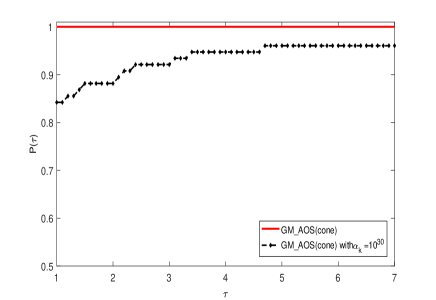
Figure 2: $N_{f}$ (80pAndr)

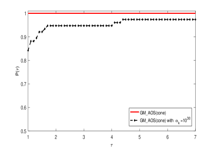
Figure 3: $N_{g}$ (80pAndr)

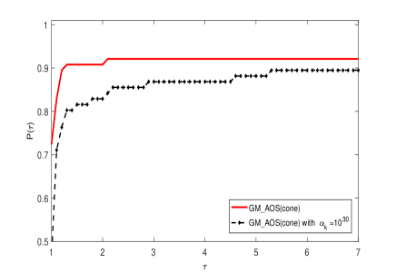
Figure 4: $T_{CPU}$ (80pAndr)

In the first group of numerical experiments, we use the collect set 80pAndr to examine the effectiveness of the stepsize (2.11). In Figs. 2-4, “GM$\_$AOS (cone) with $\alpha_{k}=10^{30}$” stands for the variant of GM$\_$AOS (cone), which is different from GM$\_$AOS (cone) only in that (2.11) is replaced by $\alpha_{k}=10^{30}$ in the Step 2.3 of GM$\_$AOS (cone). In numerical experiments, GM$\_$AOS (cone) successfully solves all 80 problems, while its variant successfully solves 76 problems. As shown in Fig. 2, GM$\_$AOS (cone) performs slightly better than its variant in term of the number of iterations. We can observe from Figs. 2-4 that GM$\_$AOS (cone) requires much less function evaluations and less gradient evaluations than its variant since the stepsize (2.11) is used. In Fig. 4, we see that GM$\_$AOS (cone) is much faster than its variant. It indicates that the stepsize (2.11) is very efficient.

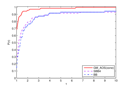
Figure 5: $N_{iter}$ (80pAndr)

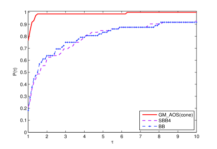
Figure 6: $N_{f}$ (80pAndr)

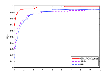
Figure 7: $N_{g}$ (80pAndr)

Figure 8: $T_{CPU}$ (80pAndr)

In the second group of numerical experiments, we also use the collect set 80pAndr to compare the performances of GM$\_$AOS (cone) with that of the SBB4 method and the BB method. In numerical experiments, GM$\_$AOS (cone) successfully solves all 80 problems, while the SBB4 method and the BB method successfully solve 75 and 76 problems, respectively. As shown in Fig. 6, GM$\_$AOS (cone) outperforms the SBB4 method and the BB method, since GM$\_$AOS (cone) successfully solves about 68$\%$ problems with the least iterations, while the percentages of the SBB4 method and the BB method are about 28$\%$ and 15$\%$, respectively. Similar observation can be made in Fig. 8 for the number of gradient evaluations. We observe from Fig. 6 that GM$\_$AOS (cone) has a very great advantage over the SBB4 method and the BB method in term of the number of function evaluations, since GM$\_$AOS (cone) successfully solves about $77\%$ problems with the least function evaluations, while the percentage of the SBB4 method and the BB method are $21\%$ and $18\%$, respectively. Fig. 8 shows that GM$\_$AOS (cone) is much faster than the SBB4 method and the BB method. It indicates that GM$\_$AOS (cone) is superior to the SBB4 method and the BB method.

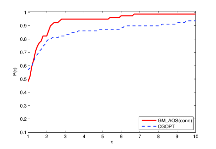
Figure 9: $N_{iter}$ (80pAndr)

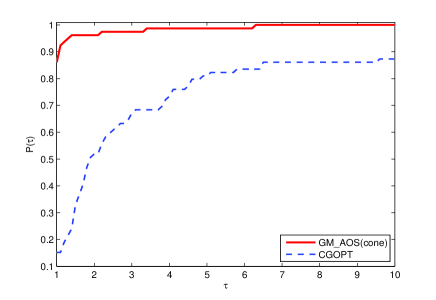
Figure 10: $N_{f}$ (80pAndr)

Figure 11: $N_{g}$ (80pAndr)

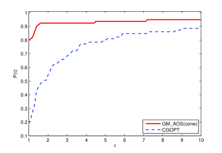
Figure 12: $T_{CPU}$ (80pAndr)

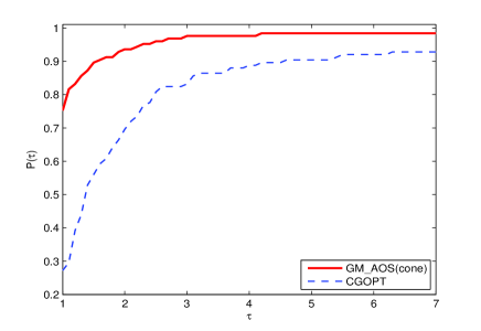
Figure 13: $N_{f}$ (144pCUTEr)

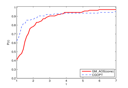
Figure 14: $N_{g}$ (144pCUTEr)

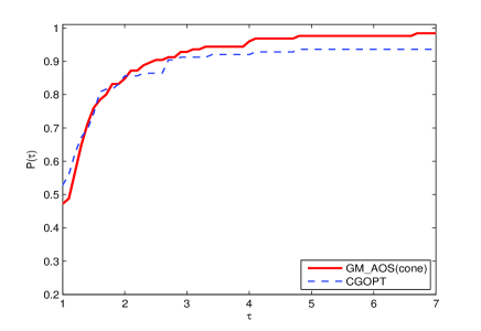
Figure 15: $N_{f}+3N_{g}$(144pCUTEr)

Figure 16: $T_{CPU}$ (144pCUTEr)

In the third group of numerical experiments, we use the collect sets 80pAndr and 144pCUTEr to compare the performance of GM$\_$AOS with that of CGOPT. For 80pAndr, GM$\_$AOS (cone) successfully solves all 80 problems, while CGOPT successfully solves 79 problems. Figs. 10-12 plot the performance profiles of GM$\_$AOS (cone) and CGOPT for 80pAndr in term of $N_{t}$, $N_{f}$, $N_{g}$ and $T_{CPU}$. As shown in Figs. 10-12, we observe that GM$\_$AOS (cone) is considerably superior to CGOPT for 80pAndr. For 144pCUTEr, GM$\_$AOS (cone) successfully solves 134 problems, while CGOPT successfully solves 133 problems. Figs. 14-16 plot the performance profiles of GM$\_$AOS (cone) and CGOPT for 144pCUTEr in term of $N_{f}$, $N_{g}$, $N_{f}+3N_{g}$ ZhangHager2006Algorithm and $T_{CPU}$. As shown in Fig. 14, GM$\_$AOS (cone) is much superior to CGOPT in term of $N_{f}$, since GM$\_$AOS (cone) solves about 78$\%$ problems with the least function evaluation, while the percentage of CGOPT is about 29$\%$ for 80pAndr. Fig. 14 indicates that GM$\_$AOS (cone) is inferior to CGOPT in term of $N_{g}$, while Fig. 16 shows that GM$\_$AOS (cone) performs a little better than CGOPT in term of $N_{f}+3N_{g}$. We observe from Fig. 16 that GM$\_$AOS (cone) is as fast as CGOPT. It indicates GM$\_$AOS (cone) is much superior to CGOPT for 80pAdr and is comparable to CGOPT for 144pCUTEr.

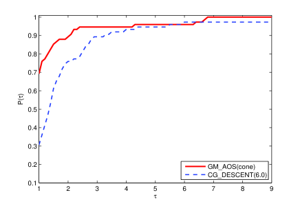
Figure 17: $N_{f}$ (80pAndr)

Figure 18: $N_{g}$ (80pAndr)

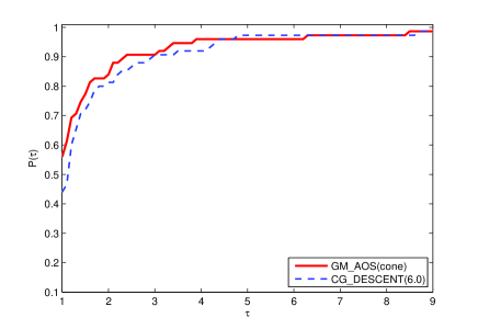
Figure 19: $N_{f}+3N_{g}$(80pAndr)

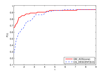
Figure 20: $T_{CPU}$(80pAndr)

In the fourth group of numerical experiments, we use the collect set 80pAndr to compare the performance of GM$\_$AOS with that of CG$\_$DESCENT (6.0), which is the limited memory conjugate gradient software package, and then use the collect set 144pCUTEr to compare the performance of GM$\_$AOS with that of CG$\_$DESCENT (5.0). For 80pAndr, GM$\_$AOS (cone) successfully solves all 80 problems, while CG$\_$DESCENT (6.0) successfully solves 75 problems. Figs. 18-20 plot the performance profiles of GM$\_$AOS (cone) and CG$\_$DESCENT (6.0) for 80pAndr in term of $N_{f}$, $N_{g}$, $N_{f}+3N_{g}$ ZhangHager2006Algorithm and $T_{CPU}$. As shown in Figs.18-18, we observe that GM$\_$AOS (cone) is considerably superior to CG$\_$DESCENT (6.0) in term of $N_{f}$ but is a little inferior to CG$\_$DESCENT (6.0) in term of $N_{g}$. Fig. 20 shows that GM$\_$AOS (cone) performs better than CG$\_$DESCENT (6.0) in term of $N_{f}+3N_{g}$. We observe from Fig. 20 that GM$\_$AOS (cone) is faster than CG$\_$DESCENT (6.0). For 144pCUTEr, GM$\_$AOS (cone) successfully solves 134 problems, while CG$\_$DESCENT (5.0) successfully solves 142 problems. Figs. 22-24 plot the performance profiles of GM$\_$AOS (cone) and CG$\_$DESCENT (5.0) for 144pCUTEr in term of $N_{f}$, $N_{g}$, $N_{f}+3N_{g}$ and $T_{CPU}$. As shown in Fig. 22, GM$\_$AOS (cone) is much superior to CGOPT in term of $N_{f}$, since GM$\_$AOS (cone) solves about 65$\%$ problems with the least function evaluations, while the percentage of CG$\_$DESCENT (5.0) is about 39$\%$. Fig. 22 indicates that GM$\_$AOS (cone) is inferior to CG$\_$DESCENT (5.0) in term of $N_{g}$, while Fig. 24 shows that GM$\_$AOS (cone) is comparable to CG$\_$DESCENT (5.0) in term of $N_{f}+3N_{g}$. We observe from Fig. 24 that GM$\_$AOS (cone) is as fast as CG$\_$DESCENT (5.0). It indicates GM$\_$AOS (cone) is superior to CG$\_$DESCENT (6.0) for 80pAdr and is comparable to CG$\_$DESCENT (5.0) for 144pCUTEr.

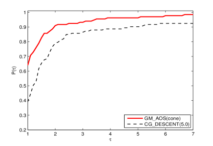
Figure 21: $N_{f}$ (144pCUTEr)

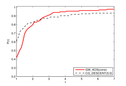
Figure 22: $N_{g}$ (144pCUTEr)

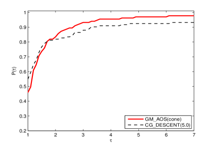
Figure 23: $N_{f}+3N_{g}$(144pCUTEr)

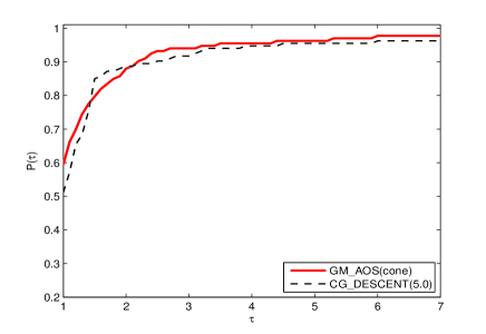
Figure 24: $T_{CPU}$ (144pCUTEr)

5 Conclusions and Discussions

In this paper, we present an improved gradient method with approximately optimal stepsize based on conic model (GM$\_$AOS (cone)). In GM$\_$AOS (cone), some approximation models including the conic model and some quadratic models are exploited to generate approximately optimal stepsizes for gradient method. It is noted that the main difference between the proposed method and the gradient method with approximately opitmal stepsize based on conic model Liu2018GMAOScone lies that the proposed method uses the stepsize (3.1) as the initial stepsize at the first iteration, while the gradient method Liu2018GMAOScone takes $1/\left\|g_{0}\right\|_{\infty}$ as the initial stepsize. In addition, more numerical experiments with two group collect sets 80pAdr and 144pCUTEr are conducted to examine the effectiveness of the proposed method. Numerical results indicate that GM$\_$AOS (cone) is superior to the SBB4 method and the BB method, performs better than CGOPT Dai2013CGOPT for 80pAdr and is comparable to CGOPT for 144pCUTEr, and is superior to the limited memory conjugate gradient software package CG$\_$DESCENT (6.0) HagerZhang2013The for 80pAdr

Table 1: The test functions in collect set 80pAndr mainly from Andrei2008An

Name	Name
Freudenstein and Roth FREUROTH (CUTE)	EG2 (CUTE)
Extended Trigonometric ET1	EDENSCH (CUTE)
Extended Rosenbrock SROSENBR (CUTE)	Broyden Pentadiagonal (CUTE)
Extended White and Holst	Almost Perturbed Quadratic
Extended Beale BEALE (CUTE)	Almost Perturbed Quartic
Extended Penalty	FLETCHCR (CUTE)
Perturbed Quadratic	ENGVAL1 (CUTE)
Raydan 1	DENSCHNA (CUTE)
Raydan 2	DENSCHNB (CUTE)
TR-SUMM	DENSCHNC (CUTE)
Diagonal 1	DENSCHNF (CUTE)
Diagonal 2	SINQUAD (CUTE)
Hager	HIMMELBG (CUTE)
Generalized Tridiagonal 1	HIMMELBH (CUTE)
Extended Tridiagonal 1	DIXON3DQ (CUTE)
Extended Three Expo Terms	BIGGSB1 (CUTE)
Generalized Tridiagonal 2	Perturbed Quadratic
Diagonal 3 (1c1c)	GENROSNB (CUTE)
Diagonal Full Borded	QP1 Extended Quadratic Penalty
Extended Himmelblau HIMMELBC (CUTE)	QP2 Extended Quadratic Penalty
Extended Powell	Tridiagonal TS1
Tridiagonal Double Borded Arrow Up	Tridiagonal TS2
Extended PSC1	Tridiagonal TS3
Extended Block-Diagonal BD1	Extended Trigonometric ET2
Extended Maratos	QP3 Extended Quadratic Penalty
Full Hessian FH1	EG1
Extended Cliff	GENROSEN-2
Quadratic Diagonal Perturbed	PRODsin
Full Hessian FH2	PROD1 (m=n)
Full Hessian FH3	PRODcos
Tridiagonal Double Borded - NONDQUAR	PROD2 (m=1)
Tridiagonal White and Holst (c=4)	ARGLINB (m=5)
Diagonal Double Borded Arrow Up	DIXMAANA (CUTE)
TRIDIA (CUTE)	DIXMAANB (CUTE)
ARWHEAD (CUTE)	DIXMAANC (CUTE)
NONDIA (CUTE)	DIXMAAND (CUTE)
Extended WOODS (CUTE)	DIXMAANL (CUTE)
Extended Hiebert	VARDIM (CUTE)
BDQRTIC (CUTE)	DIAG-AUP1
DQDRTIC (CUTE)	ENGVAL8

Table 2: The test functions in collect set 144pCUTEr from CUTEr library Gould2001CUTEr

Name	Dimension	Name	Dimension	Name	Dimension
AKIVA	2	EDENSCH	2000	NONDQUAR	5000
ALLINITU	4	EG2	1000	OSBORNEA	5
ARGLINA	200	EIGENALS	2550	OSBORNEB	11
ARGLINB	200	EIGENBLS	2550	OSCIPATH	10
ARWHEAD	5000	EIGENCLS	2652	PALMER1C	8
BARD	3	ENGVAL1	5000	PALMER1D	7
BDQRTIC	5000	ENGVAL2	3	PALMER2C	8
BEALE	2	ERRINROS	50	PALMER3C	8
BIGGS6	6	EXPFIT	2	PALMER4C	8
BOX3	3	EXTROSNB	1000	PALMER5C	6
BOX	10000	FLETCBV2	5000	PALMER6C	8
BRKMCC	2	FLETCHCR	1000	PALMER7C	8
BROWNAL	200	FMINSRF2	5625	PALMER8C	8
BROWNBS	2	FMINSURF	5625	PARKCH	15
BROWNDEN	4	FREUROTH	5000	PENALTY1	1000
BROYDN7D	5000	GENHUMPS	5000	PENALTY2	200
BRYBND	5000	GENROSE	500	PENALTY3	200
CHAINWOO	4000	GROWTHLS	3	POWELLSG	5000
CHNROSNB	50	GULF	3	POWER	10000
CLIFF	2	HAIRY	2	QUARTC	5000
COSINE	10000	HATFLDD	3	ROSENBR	2
CRAGGLVY	5000	HATFLDE	3	S308	2
CUBE	2	HATFLDFL	3	SCHMVETT	5000
CURLY10	10000	HEART6LS	6	SENSORS	100
CURLY20	10000	HEART8LS	8	SINEVAL	2
CURLY30	10000	HELIX	3	SINQUAD	5000
DECONVU	63	HIELOW	3	SISSER	2
DENSCHNA	2	HILBERTA	2	SNAIL	2
DENSCHNB	2	HILBERTB	10	SPARSINE	5000
DENSCHNC	2	HIMMELBB	2	SPARSQUR	10000
DENSCHND	3	HIMMELBF	4	SPMSRTLS	4999
DENSCHNE	3	HIMMELBG	2	SROSENBR	5000
DENSCHNF	2	HIMMELBH	2	STRATEC	10
DIXMAANA	3000	HUMPS	2	TESTQUAD	5000
DIXMAANB	3000	JENSMP	2	TOINTGOR	50
DIXMAANC	3000	JIMACK	3549	TOINTGSS	5000
DIXMAAND	3000	KOWOSB	4	TOINTPSP	50
DIXMAANE	3000	LIARWHD	5000	TOINTQOR	50
DIXMAANF	3000	LOGHAIRY	2	TQUARTIC	5000
DIXMAANG	3000	MANCINO	100	TRIDIA	5000
DIXMAANH	3000	MARATOSB	2	VARDIM	200
DIXMAANI	3000	MEXHAT	2	VAREIGVL	50
DIXMAANJ	3000	MOREBV	5000	VIBRBEAM	8
DIXMAANK	15	MSQRTALS	1024	WATSON	12
DIXMAANL	3000	MSQRTBLS	1024	WOODS	4000
DIXON3DQ	10000	NCB20B	5000	YFITU	3
DJTL	2	NCB20	5010	ZANGWIL2	2
DQDRTIC	5000	NONCVXU2	5000
DQRTIC	5000	NONDIA	5000

and is comparable to CG$\_$DESCENT (5.0) Hager2005A for 144pCUTEr. As far as we know, GM$\_$AOS (cone) is the most efficient gradient method for general unconstrained optimization so far.

Given that the search direction $-g_{k}$ has low storage and can be easily computed, the nonmonotone Armijo line search used can be easily implemented and the numerical effect is surprising, the gradient methods with approximately optimal stepsizes will be strong candidates for large scale unconstrained optimization. And the following problems are very interesting:(1) What is the best gradient method with approximately optimal stepsize (GM$\_$AOS) ? (2) Can the gradient method with approximately optimal stepsize perform better than CG$\_$DESCENT (5.3) for CUTEr library?

- (1) Cauchy, A.: Méthode générale pour la résolution des systéms déquations simultanées. Comp. Rend. Sci. Paris, 25, 46-89(1847).
- (2) Barzilai, J., Borwein, J.M.: Two-point step size gradient methods. IMA J. Numer. Anal. 8, 141-148(1988)
- (3) Asmundis, R. D., Serafino, D. D, Riccio, F., et al.: On spectral properties of steepest descent methods . IMA J. Numer. Anal. 33(4), 1416-1435(2013).
- (4) Raydan, M.: On the Barzilai and Borwein choice of steplength for the gradient method. IMA J. Numer. Anal. 13, 321-326(1993).
- (5) Dai, Y. H., Liao, L. Z.: -linear convergence of the Barzilai and Borwein gradient method. IMA J. Numer. Anal. 22(1), 1-10(2002).
- (6) Raydan, M.: The Barzilai and Borwein gradient method for the large scale unconstrained minimization problem. SIAM J. Optim. 7, 26-33(1997).
- (7) Grippo, L., Lampariello, F., Lucidi,S.: A nonmonotone line search technique for Newton’s method. SIAM J. Numer. Anal. 23, 707-716(1986).
- (8) Biglari, F., Solimanpur, M.: Scaling on the spectral gradient method. J. Optim. Theory Appl. 158(2), 626-635(2013).
- (9) Dai, Y. H., Yuan, J. Y., Yuan, Y.X.: Modified two-point stepsize gradient methods for unconstrained optimization problems. Comput. Optim. Appl. 22, 103-109(2002).
- (10) Yuan Y.X., Stoer J.: A subspace study on conjugate gradient algorithms. Z. Angew. Math. Mech. 75(1), 69-77(1995)
- (11) Dai. Y. H., Hager, W. W., Schittkowski, K., et al.: The cyclic Barzilai-Borwein method for unconstrained optimization. IMA J. Numer. Anal. 26(3), 604-627(2006).
- (12) Xiao, Y. H., Wang, Q. Y., Wang, D., et al.: Notes on the Dai-Yuan-Yuan modified spectral gradient method. J. Comput. Appl. Math. 234(10), 2986-2992(2010).
- (13) Miladinović, M., Stanimirović, P., Miljković, S.: Scalar correction method for solving large scale unconstrained minimization problems. J. Optim. Theory Appl. 151(2), 304-320(2011).
- (14) Zhou, B., Gao, L., Dai, Y. H.: Gradient methods with adaptive stepsizes. Comput. Optim. Appl. 35(1), 69-86 (2006).
- (15) Hager, W. W., Zhang, H. C.: A new conjugate gradient method with guaranteed descent and an efficient line search. SIAM J. Optim. 16(1), 170-192(2005).
- (16) Han, Q. M., Sun, W. Y., Han, J. Y., et al.: An adaptive conic trust-region method for unconstrained optimization. Optim. Methods Softw. 20(6), 665-677(2005).
- (17) Sun, W.Y., Xu, D.: A filter-trust-region method based on conic model for unconstrained optimization (in Chinese). Sci. Sin. Math 55(5), 527-543 (2012)
- (18) Yuan, Y. X., Sun, W. Y.: Theory and methods of optimization. Science Press of China (1999).
- (19) Sun, W.Y.: Optimization methods for non-quadratic model. Asia-Pac. J. Oper. Res. 13(1), (1996)
- (20) Davidon, W. C.: Conic Approximations and Collinear Scalings for Optimizers. SIAM J. Numer. Anal. 17(2), 268-281(1980).
- (21) Sorensen, D. C.: The Q-Superlinear Convergence of a Collinear Scaling Algorithm for Unconstrained Optimization. SIAM J. Numer. Anal. 17(17), 84-114(1980).
- (22) Zhang, J. Z., Deng, N. Y., Chen, L. H.: New quasi-Newton equation and related methods for unconstrained optimization. J. Optim. Theory Appl. 102, 147-167 (1999).
- (23) Friedlander, A., Martinez, J. M., Molina, B., et al. Gradient Method with Retards and Generalizations. SIAM J. Numer. Anal. 36(1), 275-289(1998).
- (24) Zhang, H. C., Hager, W. W.: A nonmonotone line search technique and its application to unconstrained optimization. SIAM J. Optim. 14, 1043-1056(2004).
- (25) Birgin, E. G., Martínez, J. M., Raydan, M.: Nonmonotone spectral projected gradient methods for convex sets. SIAM J. Optim. 10(4), 1196-1211(2000).
- (26) Dai, Y. H., Kou, C. X.: A nonlinear conjugate gradient algorithm with an optimal property and an improved Wolfe line search. SIAM J. Optim. 23(1), 296-320(2013)
- (27) Andrei, N.: An unconstrained optimization test functions collection. Adv. Model. Optim. 10, 147-161(2008).
- (28) Gould, N. I. M., Orban, D., Toint, Ph.L.: CUTEr and SifDec: A constrained and unconstrained testing environment, revisited. ACM Trans. Math. Softw. 29(4), 373-394(2003).
- (29) Hager, W.W., Zhang, H. C.: The limited memory conjugate gradient method. SIAM J. Optim. 23(4), 2150-2168(2013)
- (30) Liu, Z. X., Liu, H. W., Dong, X. L.: An efficient gradient method with approximate optimal stepsize for the strictly convex quadratic minimization problem. Optimization 67(3), 427-440(2018).
- (31) Liu, Z. X., Liu, H. W.: An efficient gradient method with approximate optimal stepsize for large-scale unconstrained optimization. Numer. Algorithms 78(1), 21-39(2018).
- (32) Liu, Z. X., Liu, H. W.: Several efficient gradient methods with approximate optimal stepsizes for large scale unconstrained optimization. J. Comput. Appl. Math. 328, 400-413(2018).
- (33) Liu, Z. X., Liu, H. W.: An efficient gradient methods with approximately optimal stepsizes based on tensor model for unconstrained optimization. J. Optim. Theory Appl. 181(2), 608-633(2019).
- (34) Liu, H. W., Liu, Z. X., Dong, X. L.: A new adaptive Barzilai and Borwein method for unconstrained optimization. Optim. Lett. 12(4), 845-873(2018).
- (35) Snezana S Djordjevic. Some unconstrained optimization methods, In Applied Mathematics. DOI:10.5772/intechopen.83679, 2019.
- (36) Liu, H. W., Liu, H. X.: An efficient Barzilai-Borwein conjugate gradient method for unconstrained optimization. J. Optim. Theory Appl. 180(3), 879-906(2019).
- (37) Dolan, E. D., Moré, J. J.: Benchmarking optimization software with performance profiles. Math. Program. 91, 201-213(2002).
- (38) Hager, W. W., Zhang, H.C.: Algorithm 851:CGDESCENT, a conjugate gradient method with guaranteed descent. ACM Trans. Math. Softw. 32(1), 113-137(2006).