Single-use automata and transducers for infinite alphabets

Abstract

Our starting point are register automata for data words, in the style of Kaminski and Francez. We study the effects of the single-use restriction, which says that a register is emptied immediately after being used. We show that under the single-use restriction, the theory of automata for data words becomes much more robust. The main results are: (a) five different machine models are equivalent as language acceptors, including one-way and two-way single-use register automata; (b) one can recover some of the algebraic theory of languages over finite alphabets, including a version of the Krohn-Rhodes Theorem; (c) there is also a robust theory of transducers, with four equivalent models, including two-way single use transducers and a variant of streaming string transducers for data words. These results are in contrast with automata for data words without the single-use restriction, where essentially all models are pairwise non-equivalent.

1 Introduction

One of the appealing features of regular languages for finite alphabets is the robustness of the notion: it can be characterised by many equivalent models of automata (one-way, two-way, deterministic, nondeterministic, alternating, etc.), regular expressions, finite semigroups, or monadic second-order logic. A similar robustness appears for transducers, see [16] for a survey; particularly for the class of regular string-to-string functions, which can be characterised using deterministic two-way transducers, streaming string transducers, or mso transductions.

This robustness vanishes for infinite alphabets. We consider infinite alphabets that are constructed using an infinite set $\mathbb{A}$ of atoms, also called data values. Atoms can only be compared for equality. The literature for infinite alphabets is full of depressing diagrams like [22, Figure 1] or [7, p. 24], which describe countless models that satisfy only trivial relationships such as deterministic $\subseteq$ nondeterministic, one-way $\subseteq$ two-way, etc.

This lack of robustness has caused several authors to ask if there is a notion of “regular language” for infinite alphabets; see [4, p. 703] or [5, p. 2]. This question was probably rhetorical, with the assumed answer being “no”. In this paper, we postulate a “yes” answer. The main theme is register automata, as introduced by Kaminski and Francez [19], but with the single-use restriction, which says that immediately after a register is used, its value is destroyed. As we show in this paper, many automata constructions, which fail for unrestricted register automata, start to work again in the presence of the single-use restriction.

Before describing the results in the paper, we illustrate the single-use restriction.

Example 1. Consider the language “there are at most three distinct letters in the input word, not counting repetitions”, over alphabet $\mathbb{A}$. There is a natural register automaton which recognises this language: use three registers to store the distinct atoms that have been seen so far, and if a fourth atom comes up, then reject. This automaton, however, violates the single-use restriction, because each new input letter is compared to all the registers.

Here is a solution that respects the single-use restriction. The idea is that once the automaton has seen three distinct letters $a,b,c$, it stores them in six registers as explained in the picture on the right. Assume that a new input letter $d$ is read. The behaviour of the automaton (when it already has three atoms in its registers) is explained in the flowchart in Figure 1.

A similar flowchart is used for the corner cases when the automaton has seen less than three letters so far.

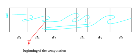
Figure 1: Updating the six registers.

$\Box$

Our first main result, Theorem 3.3 (in Section 3), says that the following models recognise the same languages over infinite alphabets:

1. deterministic one-way single-use automata;

2. deterministic two-way single-use automata;

3. orbit-finite monoids [6];

4. rigidly guarded mso^∼ [13];

5. string-to-boolean regular list functions with atoms.

The equivalence of the models in items 3 and 4 was shown in [13]; the remaining models and their equivalences are new (item 5 is an extension of the regular list functions from [9]).

Just like their classical versions, one-way and two-way single-use automata are equivalent as language acceptors, but they are no longer equivalent as transducers. For example, a two-way single-use transducer can reverse the input string, which is impossible for a one-way single-use transducer. In Sections 4 and 5 we develop the theory of single-use transducers:

In Section 4, we investigate single-use one-way transducers. For finite alphabets, one of the most important results about one-way transducers is the Krohn-Rhodes Theorem [21], which says that every Mealy machine (which is a length preserving one-way transducer) can be decomposed into certain “prime” Mealy machines. We show that the same can be done for infinite alphabets, using a single-use extension of Mealy machines. The underlying prime machines are the machines from the original Krohn-Rhodes theorem, plus one additional register machine which moves atoms to later positions.

In Section 5, we investigate single-use two-way transducers, and show that the corresponding class of string-to-string functions enjoys similar robustness properties as the languages discussed in Theorem 3.3, with four models being equivalent:

1. single-use two-way transducers;

2. an atom extension of streaming string transducers [2];

3. string-to-string regular list functions with atoms;

4. compositions of certain “prime two-way machines” (Krohn & Rhodes style).

We also show other good properties of the string-to-string functions in the above items, including closure under composition (which follows from item 4) and decidable equivalence.

Summing up, the single-use restriction allows us to identify languages and string-to-string functions with infinite alphabets, which share the robustness and good mathematical theory usually associated with regularity for finite alphabets.

Due to space constraints, and a large number of results, virtually all of the proofs are in an appendix. We use the available space to explain and justify the many new models that are introduced.

2 Automata and transducers with atoms

For the rest of the paper, fix an infinite set $\mathbb{A}$, whose elements are called atoms. Atoms will be used to construct infinite alphabets. Intuitively speaking, atoms can only be compared for equality. It would be interesting enough to consider alphabets of the form $\mathbb{A}\times\Sigma$, for some finite $\Sigma$, as is typically done in the literature on data words [5, p. 1]. However, in the proofs, we use more complicated sets, such as the set $\mathbb{A}^{2}$ of pairs of atoms, the set $\mathbb{A}+\{\vdash,\dashv\}$ obtained by adding two endmarkers to the atoms, or the co-product (i.e. disjoint union) $\mathbb{A}^{2}+\mathbb{A}^{3}$. This motivates the following definition.

Definition 2.1.

A polynomial orbit-finite set is any set that can be obtained from $\mathbb{A}$ and singleton sets by means of finite products and co-products (i.e. disjoint unions).

We only care about properties of such sets that are stable under atom automorphisms, as described below. Define an atom automorphism to be any bijection $\mathbb{A}\to\mathbb{A}$. (This notion of automorphism formalises the intuition that atoms can only be compared for equality). Atom automorphisms form a group. There is a natural action of this group on polynomial orbit-finite sets: for elements of $\mathbb{A}$ we apply the atom automorphism, for singleton sets the action is trivial, and for other polynomial orbit-finite sets the action is lifted inductively along $+$ and $\times$ in the natural way. Let $\Sigma$ and $\Gamma$ be sets equipped with an action of the group of atom automorphisms – in particular, these could be polynomial orbit-finite sets. A function $f:\Sigma\to\Gamma$ is called equivariant if $f(\pi(x))=\pi(f(x))$ holds for every $x\in\Sigma$ and every atom automorphism $\pi$. The general idea is that equivariant functions can only talk about equality of atoms. In the case of polynomial orbit-finite sets, equivariant functions can also be finitely represented using quantifier-free formulas [7, Lemma 1.3].

The model. We now describe the single-use machine models discussed in this paper. There are four variants: machines can be one-way or two-way, and they can recognise languages or compute string-to-string functions. We begin with the most general form – two-way string-to-string functions – and define the other models as special cases.

The machine reads the input string, extended with left and right endmarkers $\vdash,\dashv$. It uses registers to store atoms that appear in the input string. A register can store either an atom, or the undefined value $\bot$. The single-use restriction, which is written in red below, says that a register is set to $\bot$ immediately after being used.

Definition 2.2.

The syntax of a two-way single-use transducer consists of

• input and output alphabets $\Sigma$ and $\Gamma$, both polynomial orbit-finite sets;

• a finite set of states $Q$, with a distinguished initial state $q_{0}\in Q$;

• a finite set $R$ of register names;

• a transition function which maps each state $q\in Q$ to an element of:

  $$\underbrace{\text{questions}}_{\text{question that is asked}}\times\underbrace{(Q\times\text{actions})}_{\begin{subarray}{c}\text{what to do if the}\\ \text{question has a yes answer}\end{subarray}}\times\underbrace{(Q\times\text{actions})}_{\begin{subarray}{c}\text{what to do if the}\\ \text{question has a no answer}\end{subarray}}$$

  where the allowed questions and actions are taken from the following toolkit:

  1. Questions.

     1. Apply an equivariant function $f:\Sigma+\{\vdash,\dashv\}\to\{\text{yes, no}\}$ to the letter under the head, and return the answer.

     2. Are the atoms stored in registers $r_{1},r_{2}$ equal and defined? If any of these registers is undefined, then the run immediately stops and rejects. This question has the side effect of setting the values of $r_{1}$ and $r_{2}$ to $\bot$.

  2. Actions.

     1. Apply an equivariant function $f:\Sigma+\{\vdash,\dashv\}\to\mathbb{A}+\bot$ to the letter under the head, and store the result in register $r\in R$.

     2. Apply an equivariant function $f:\mathbb{A}^{k}\to\Gamma$ to the contents of distinct registers $r_{1},\ldots,r_{k}\in R$, and append the result to the output string. If any of the registers is undefined, stop and reject. This action has the side effect of setting the values of $r_{1},r_{2},\ldots,r_{k}$ to $\bot$.

     3. Move the head to the previous/next input position.

     4. Accept/reject and finish the run.

The semantics of the transducer is a partial function from strings over the input alphabet to strings over the output alphabet. Consider a string of the form $\vdash\!\!w\!\!\dashv$ where $w\in\Sigma^{*}$. A configuration over such a string consists of (a) a position in the string; (b) a state; (c) a register valuation, which is a function of type $R\to\mathbb{A}+\bot$; (d) an output string, which is a string over the output alphabet. A run of the transducer is defined to be a sequence of configurations, where consecutive configurations are related by applying the transition function in the natural way. The output of a run is defined to be the contents of the output string in the last configuration. An accepting configuration is one which executes the accept action from item 2d – accepting configurations have no successors. The initial configuration is a configuration where the head is over the left endmarker $\vdash$, the state is the initial state, the register valuation maps all registers to the undefined value, and the output string is empty. An accepting run is a run that begins in the initial configuration and ends in an accepting one. By determinism, there is at most one accepting run. The semantics of the transducer is defined to be the partial function $\Sigma^{*}\to\Gamma^{*}$, which inputs $w\in\Sigma^{*}$ and returns the output of the accepting run over $\vdash\!\!w\!\!\dashv$. If there is no accepting run, $f(w)$ has no value.

Special cases. A one-way single-use transducer is the special case of Definition 2.2 which does not use the “previous” action from item 2c. A two-way single-use automaton is the special case which does not use the output actions from item 2b. The language recognised by such an automaton is defined to be the set of words which admit an accepting run. A one-way single-use automaton is the special case of a two-way single-use automaton, which does not use the “previous” action from item 2c.

3 Languages recognised by single-use automata

In this section we discuss languages recognised by single-use automata. The main result is that one-way and two-way single-use automata recognise the same languages, and furthermore these are the same languages that are recognised by orbit-finite monoids [6], the logic rigidly guarded mso^∼ [13], and a new model called regular list functions with atoms, that will be defined in Section 5.

Orbit-finite monoids. We begin by defining orbit-finite sets and orbit-finite monoids, which play an important technical role in this paper. For more on orbit-finite sets, see the lecture notes [7]. For a tuple $\bar{a}\in\mathbb{A}^{*}$, an $\bar{a}$-automorphism is defined to be any atom automorphism that maps $\bar{a}$ to itself. Consider set $X$ equipped with an action of the group of atom automorphisms. We say that $x\in X$ is supported by a tuple of atoms $\bar{a}\in\mathbb{A}^{*}$ if $\pi(x)=x$ holds for every $\bar{a}$-automorphism $\pi$. We say that a subset of $X$ is $\bar{a}$-supported if it is an $\bar{a}$-supported element of the powerset of $X$; similarly we define supports of relations and functions. We say that $x$ is finitely supported if it is supported by some tuple $\bar{a}\in\mathbb{A}^{*}$. Define the $\bar{a}$-orbit of $x$ to be its orbit under the action of the group of $\bar{a}$-automorphisms.

Definition 3.1 (Orbit-finite sets).

Let $X$ be a set equipped with an action of atom automorphisms. A subset $Y\subseteq X$ is called orbit-finite if (a) every element of $Y$ is finitely supported; and (b) there exists some $\bar{a}\in\mathbb{A}^{*}$ such that $Y$ is a union of finitely many $\bar{a}$-orbits.

An equivariant orbit-finite set is the special case where the tuple $\bar{a}$ in item (b) is empty. The polynomial orbit-finite sets from Section 2 are a special case of equivariant orbit-finite sets. The following notion was introduced in [6, Section 3].

Definition 3.2 (Orbit-finite monoid).

An orbit-finite monoid is a monoid where the underlying set is orbit-finite, and the monoid operation is finitely supported. Let $\Sigma$ be an orbit-finite set. We say that a language $L\subseteq\Sigma^{*}$ is recognised by an orbit-finite monoid $M$ if there is a finitely supported monoid morphism $h:\Sigma^{*}\to M$ and a finitely supported accepting set $F\subseteq M$ such that $L$ contains exactly the words whose image under $h$ belongs to $F$.

In this paper, we are mainly interested in the case where both the morphism and the accepting set are equivariant. In this case, it follows that the alphabet $\Sigma$, the image of the morphism, and the recognised language all also have to be equivariant.

The structural theory of orbit-finite monoids was first developed in [6], where it was shown how the classical results about Green’s relations for finite monoids extend to the orbit-finite setting. This theory was further investigated in [13], including a lemma stating that every orbit-finite group is necessarily finite. In the appendix of this paper we build on these results, to prove an orbit-finite version of the Factorisation Forest Theorem of Simon [26, Theorem 6.1], which is used in proofs of Theorems 3.3 and 4.2.

Main theorem about languages. We are now ready to state Theorem 3.3, which is our main result about languages.

Theorem 3.3.

Let $\Sigma$ be a polynomial orbit-finite set. The following conditions are equivalent for every language $L\subseteq\Sigma^{*}$:

1. $L$ is recognised by a single-use one-way automaton;

2. $L$ is recognised by a single-use two-way automaton;

3. $L$ is recognised by an orbit-finite monoid, with an equivariant morphism and an equivariant accepting set;

4. $L$ can be defined in the rigidly guarded mso^∼ logic;

5. $L$’s characteristic function $\Sigma^{*}\to\{yes,no\}$ is an orbit-finite regular list function.

The equivalence of items 4 and 3 has been proved in [13, Theorems 4.2 and 5.1], and since we do not use rigidly guarded mso^∼ outside of the this theorem, we do not give a definition here (see [13, Section 3]). The orbit-finite regular list functions from item 5 will be defined in Section 5. The proof outline for Theorem 3.3 is given in the following diagram

All equivalences in the theorem are effective, i.e. there are algorithms implementing the conversions between any of the models.

The single-use restriction is crucial in the theorem. Automata without the single-use restriction – call them multiple-use – only satisfy the trivial inclusions:

$$\text{single-use}\!\!\!\!\stackrel{{\scriptstyle\hbox{\hbox{\kern 0.0pt\raise-6.6111pt\vbox{\halign{\relax\hfil\txtline@@{#}\hfil\cr\hbox{{\ignorespaces\leavevmode\scriptsize first letter appears again}\\\hbox{{\ignorespaces\scriptsize\cite[cite]{[\@@bibref{}{bojanczyk_slightly2018}{}{}, Exercise 91]}}\crcr}}}}}}{{\subsetneq}}\!\!\!\!\text{one-way multiple-use}\!\!\!\!\stackrel{{\scriptstyle\hbox{\hbox{\kern 0.0pt\raise-6.6111pt\vbox{\halign{\relax\hfil\txtline@@{#}\hfil\cr\hbox{{\ignorespaces\leavevmode\scriptsize some letter appears twice}\\\hbox{{\ignorespaces\scriptsize\cite[cite]{[\@@bibref{}{kaminskiFiniteMemoryAutomata1994}{}{}, Example 11]}}\crcr}}}}}}{{\subsetneq}}\!\!\!\!\text{two-way multiple-use}.}}}}$$

Two-way multiple-use automata have an undecidable emptiness problem [22, Theorem 5.3]. For one-way (even multiple-use) automata, emptiness is decidable and even tractable in a suitable parametrised understanding [7, Corollary 9.12]. We leave open the following question: given a one-way multiple-use automaton, can one decide if there is an equivalent automaton that is single-use (by Theorem 3.3, it does not matter whether one-way or two-way)?

3.1 From two-way automata to orbit-finite monoids

In this section, we show the implication 2 $\Rightarrow$ 3 of Theorem 3.3. (This is the only proof of the paper that is not relegated to the appendix – we chose it, because it illustrates the importance of the single-use restriction). The implication states that the language of every single-use two-way automaton can also be recognised by an equivariant homomorphism into an orbit-finite monoid. In the proof, we use the Shepherdson construction for two-way automata [25] and show that, thanks to the single-use restriction, it produces monoids which are orbit-finite.

Consider a two-way single-use automaton, with $k$ registers and let $Q$ be the set of its states. For a string over the input alphabet (extended with endmarkers), define its Shepherdson profile to be the function of the type

$$\overbrace{Q\times(\mathbb{A}+\bot)^{k}}^{\begin{subarray}{c}\text{state and register}\\ \text{valuation at the}\\ \text{start of the run}\end{subarray}}\times\overbrace{\{\leftarrow,\rightarrow\}}^{\begin{subarray}{c}\text{does the run}\\ \text{enter from the}\\ \text{left or right}\end{subarray}}\qquad\to\qquad\{\text{accept, loop}\}+(\overbrace{Q\times(\mathbb{A}+\bot)^{k}}^{\begin{subarray}{c}\text{state and register}\\ \text{valuation at the}\\ \text{end of the run}\end{subarray}}\times\overbrace{\{\leftarrow,\rightarrow\}}^{\begin{subarray}{c}\text{does the run}\\ \text{exit from the}\\ \text{left or right}\end{subarray}})$$

that describes runs of the automaton in the natural way (see [25, Proof of Theorem 2]). The run is taken until the automaton either exits the string from either side, accepts, or enters an infinite loop. By the same reasoning as in Shepherdson’s proof, one can equip the set of Shepherdson profiles with a monoid structure so that the function which maps a word to its Shepherdson profile becomes a monoid homomorphism. We use the name Shepherdson monoid for the resulting monoid (it only contains the ‘achievable’ profiles – the image of $\Sigma^{*}$). It is easy to see that whether a word is accepted depends only on an equivariant property of its Shepherdson profile, and therefore the language recognised by the automaton is also recognised by the Shepherdson monoid.

It remains to show that the Shepherdson monoid is orbit-finite, which is the main part of the proof. Unlike the arguments so far, this part of the proof relies on the single-use restriction. To illustrate this, we give an example of a one-way automaton that is not single-use and whose Shepherdson monoid is not orbit-finite.

Example 2. Consider the language over $\mathbb{A}$ of words whose first letter appears again. This language is not recognised by any orbit-finite monoid [7, Exercise 91], but it is recognised by a multiple-use one-way automaton, which stores the first letter in a register, and then compares this register with all remaining letters of the input word. For this automaton, the Shepherdson profile needs to remember all of the distinct letters that appear in the word. In particular, if two words have different numbers of distinct letters, then their Shepherdson profiles cannot be in the same orbit. Since input strings can contain arbitrarily many distinct letters, the Shepherdson monoid of this automaton is not orbit-finite. $\Box$

Lemma 3.4.

For every single-use two-way automaton there is some $N\in\mathbb{N}$ such that every Shepherdson profile is supported by at most $N$ atoms.

Before proving the lemma, we use it to show that the Shepherdson monoid is orbit-finite. In Section A of the appendix, we show that if an equivariant set consists of functions from one orbit-finite set to another orbit-finite set (as is the case for the underling set in the Shepherdson monoid) and all functions in the set have supports of bounded size (as is the case thanks to Lemma 3.4), then the set is orbit-finite. This leaves us with proving Lemma 3.4.

Proof 3.5.

Define a transition in a run to be a pair of consecutive configurations. Each transition has a corresponding question and action. A transition in a run is called important if its question or action involves a register that has not appeared in any action or question of the run. The number of important transitions is bounded by $k$ – the number of registers. The crucial observation, which relies on the single-use restriction, is that if the input word, head position, and state are fixed (but not the register valuation), then the sequence of actions in the corresponding run depends only on the answers to the questions in the important transitions. This is described in more detail below.

Fix a choice of the following parameters: (a) a string over the input alphabet that might contain endmarkers; (b) an entry point of the automaton – either the left or the right end of the word; (c) a state of the automaton. We do not fix the register valuation. For a register valuation $\eta$, define $\rho(\eta)$ to be the run which begins in the configuration described by the parameters (abc) together with $\eta$, and which is maximal, i.e. it ends when the automaton either accepts, rejects, or tries to leave the fixed string. For $i\in\{0,1,\ldots,k\}$ define $\alpha_{i}(\eta)$ to be the sequence of actions that are performed in the maximal prefix of the run $\rho(\eta)$ which uses at most $i$ important transitions. The crucial observation that was stated at the beginning of this proof is that once the parameters (abc) are fixed, then the sequence of actions $\alpha_{i}(\eta)$ depends only on the answers to the questions asked in the first $i$ important transitions. In particular, the function $\alpha_{i}$ has at most $2^{i}$ possible values. Furthermore, by a simple induction on $i$, one can show the following claim.

Claim 1.

The function $\alpha_{i}$ is supported by at most $2^{i+1}$ atoms.

Since there are at most $k$ important transitions in a run, the above claim implies that, for every fixed choice of parameters (abc), at most $2^{k+1}$ atoms are needed to support the function which maps $\eta$ to the sequence of actions in the run $\rho(\eta)$. In the arguments for the Shepherdson profile for a fixed word $w$, parameter (b) can have two values (first or last position) and parameter (c) can have at most $|Q|$ values. Therefore, at most $2|Q|2^{k+1}$ atoms are needed to support the function which takes an argument as in the Shepherdson profile, and returns the sequence of actions in the corresponding run. The lemma follows.

4 A Krohn-Rhodes decomposition of one-way transducers with atoms

In this section, we present a decomposition result for single-use one-way transducers, which is a version of the celebrated Krohn-Rhodes Theorem [21, p. 454]. We think that this result gives further evidence for the good structure of single-use models. In the next section, we give a similar decomposition result for two-way single-use transducers which will be used to prove the equivalence of several other characterisations of the two-way model.

We begin by describing the classical Krohn-Rhodes Theorem. A Mealy machine is a deterministic one-way length-preserving transducer, which is obtained from a deterministic finite automaton by labelling transitions with output letters and ignoring accepting states. The Krohn-Rhodes Theorem says that every function computed by a Mealy machine is a composition of functions computed by certain prime Mealy machines (which are called reversible and reset in [1, Chapter 6]). In this section, we prove a version of this theorem for orbit-finite alphabets; this version relies crucially on the single-use restriction. To distinguish the original model of Mealy machines from the single-use model described below, we will use the name classical Mealy machine for the Mealy machines in the original Krohn-Rhodes Theorem, i.e. the alphabets and state spaces are finite.

Define a single-use Mealy machine to have the same syntax as in Definition 2.2, with the following differences: there are no “next/previous” actions from item 2c, but the output action from item 2b has the side effect of moving the head to the next position. A consequence is that a Mealy machine is length-preserving, i.e. it outputs exactly one letter for each input position. Furthermore, there are no endmarkers and no “accept” or “reject” actions from item 2d; the automaton begins in the first input position and accepts immediately once its head leaves the input word from the right.

Example 3. Define atom propagation to be the following length-preserving function. The input alphabet is $\mathbb{A}+\{\epsilon,\downarrow\}$ and the output alphabet is $\mathbb{A}+\bot$. If a position $i$ in the input string has label $\downarrow$ and there is some (necessarily unique) position $j<i$ with an atom label such that all positions strictly between $j$ and $i$ have label $\epsilon$, then the output label of position $i$ is the atom in input position $j$. For all other input positions, the output label is $\bot$. Here is an example of atom propagation:

$$\begin{array}[]{rccccccccccccccccccc}\text{input}&1&2&\epsilon&\epsilon&\downarrow&\downarrow&3&\epsilon&\epsilon&\downarrow&\epsilon&\downarrow\\ \text{output}&\bot&\bot&\bot&\bot&2&\bot&\bot&\bot&\bot&3&\bot&\bot\end{array}$$

Atom propagation is computed by a single-use Mealy machine, which stores the most recently seen atom in a register, and outputs the register at the nearest appearance of $\downarrow$. $\Box$

The following example illustrates some of the technical difficulties with single-use Mealy machines: It is often useful to consider a Mealy machine that computes the run of another Mealy machine – it decorates every input position with the state and the register valuation that the Mealy machine will have after reading the input up to (but not including) that position. The following example shows that the single-use restriction makes this construction impossible.

Example 4.1.

Consider the single-use Mealy machine that implements the atom propagation function from Example 4. This machine has only one register. Every time it sees an atom value, it stores the value in the register and every time it sees $\downarrow$, and the register is non-empty, the machine outputs the register’s content. We claim that the run of this machine cannot be computed by a Mealy machine. If it could, we would be able to use it to construct a Mealy machine that given a word over $\mathbb{A}$, equips every position with the atom from the first position. This would easily lead to a construction of a single-use automaton for the language “the first letter appears again” (from Example 3.1) which, as we already know, is impossible.

The Krohn-Rhodes Theorem, both in its original version and in our orbit-finite version below, says that every Mealy machine can be decomposed into prime functions using two types of composition:

$$\Sigma^{*}\stackrel{{\scriptstyle g\circ f}}{{\longrightarrow}}\Delta^{*}\lx@proof@logical@and\Sigma^{*}\stackrel{{\scriptstyle f}}{{\longrightarrow}}\Gamma^{*}\Gamma^{*}\stackrel{{\scriptstyle g}}{{\longrightarrow}}\Delta^{*}\qquad(\Sigma_{1}\times\Sigma_{2})^{*}\stackrel{{\scriptstyle f_{1}|f_{2}}}{{\longrightarrow}}(\Gamma_{1}\times\Gamma_{2})^{*}\lx@proof@logical@and\Sigma_{1}^{*}\stackrel{{\scriptstyle f_{1}}}{{\longrightarrow}}\Gamma_{1}^{*}\Sigma_{2}^{*}\stackrel{{\scriptstyle f_{2}}}{{\longrightarrow}}\Gamma_{2}^{*}$$

The sequential composition is simply function composition. The parallel composition – which only makes sense for length preserving functions – applies the function $f_{i}$ to the $i$-th projection of the input string.

Theorem 4.2.

Every total function computed by a single-use Mealy machine can be obtained, using sequential and parallel composition, from the following prime functions:

1. Length-preserving homomorphisms. Any function of type $\Sigma^{*}\to\Gamma^{*}$, where $\Sigma$ and $\Gamma$ are polynomial orbit-finite, obtained by lifting to strings an equivariant function of type $\Sigma\to\Gamma$.

2. Classic Mealy machines. Any function computed by a classical Mealy machine.

3. Atom propagation. The atom propagation function from Example 4.

By the original Krohn-Rhodes theorem, classical Mealy machines can be further decomposed.

Define a composition of primes to be any function that can be obtained from the prime functions by using a parallel and sequential composition. In this terminology, Theorem 4.2 says that every function computed by a single-use Mealy machine is a composition of primes. The converse is also true: every prime function is computed by a single-use Mealy machine, and single-use Mealy machines are closed under both kinds of composition (for details see Section C of the appendix).

Decomposition of single-use one-way transducers. A Mealy machine is the special case of a single-use one-way transducer which is length preserving, and does not see an endmarker. A corollary of Theorem 4.2 is that, in order to generate all total functions computed by single-use one-way transducers, it is enough to add two items to the list of prime functions from Theorem 4.2: (a) a function $w\mapsto w\!\!\dashv$ which appends an endmarker, and (b) equivariant homomorphisms over polynomial orbit-finite alphabets that are not necessarily length-preserving.

5 Two-way single-use transducers

In this section, we turn to two-way single-use transducers. For them, we show three other equivalent models: (a) compositions of certain two-way prime functions; (b) an atom variant of the streaming string transducer (sst) model of Alur and Černý from [2]; and (c) an atom variant of the regular string functions from [9]. We believe that the atom variants of items (b) and (c), as described in this section, are the natural atom extensions of the original models; and the fact that these extensions are all equivalent to single-use two-way transducers is a further validation of the single-use restriction.

We illustrate the transducer models using the functions from the following example.

Example 4. Consider some polynomial orbit-finite alphabet $\Sigma$. The input and output alphabets are the same, namely $\Sigma$ extended with a separator symbol $|$. Define map reverse (respectively, map duplicate) to be the function which reverses (respectively, duplicates) every string between consecutive separators, as in the following examples:

$$\underbrace{12||345|678|9\ \mapsto\ 21||543|876|9}_{\text{map reverse}}\qquad\underbrace{12||345|678|9\ \mapsto\ 1212||345345|678678|99}_{\text{map duplicate}}$$

Both functions can be computed by single-use two-way transducers. These functions will be included in the prime functions for two-way single-use transducers, as discussed in item (a) at the beginning of this section. $\Box$

Streaming string transducers with atoms. A streaming string transducer with atoms has two types of registers: atom registers $r,s,\ldots$ which are the same as in Definition 2.2, and string registers $A,B,C,\ldots$ which are used to store strings over the output alphabet. Both kinds of registers are subject to the single-use restriction, which is coloured red in the following definition.

Definition 5.1 (Streaming string transducer with atoms).

Define the syntax of a streaming string transducer (sst) with atoms in the same way as a one-way single-use transducer (variant of Definition 2.2), except that the model is additionally equipped with a finite set of string registers, with a designated output string register. The actions are the same as for one-way single-use transducers except that the output action is replaced by two kinds of actions:

1. Apply an equivariant function $f:\mathbb{A}^{k}\to\Gamma$ to the contents of distinct registers $r_{1},\ldots,r_{k}\in R$, and put the result into string register $A$ (overwriting its previous contents). If any of these registers is undefined, then the run immediately stops and rejects. This action has the side effect of setting the values of $r_{1},r_{2},\ldots,r_{k_{j}}$ to $\bot$.

2. Concatenate string registers $A$ and $B$, and put the result into string register $C$. This action has the side effect of setting $A$ and $B$ to the empty string.

The output of a streaming string transducer is defined to be the contents of the designated output register when the “accept” action is performed. In the atomless case, when no atom registers are allowed and the input and output alphabets are finite, the above definition is equivalent to the original definition of streaming string transducers from [2].

Example 5. Consider the map reverse function from Example 5, with alphabet $\mathbb{A}$. To compute it, we use two string registers $A$ and $B$, with the output register being $B$. When reading an atom $a\in\mathbb{A}$, the transducer executes an action $A:=aA$. (This action needs to be broken into simpler actions as in Definition 5.1 and requires auxiliary registers). When reading a separator symbol, the automaton executes action $B:=B|A$, which erases the content of register $A$. Similar idea works for map duplicate – it uses two copies of register $A$. $\Box$

Regular list functions with atoms. Our last model is based on the regular list functions from [9]. Originally, the regular list functions were introduced to characterise two-way transducers (over finite alphabets), in terms of simple prime functions and combinators [9, Theorem 6.1]. The following definition extends the original definition in only two ways: we add an extra datatype $\mathbb{A}$ and an equality test $\mathtt{eq}:\mathbb{A}^{2}\to\{\text{yes,no}\}$.

Definition 5.2 (Regular list functions with atoms).

Define the datatypes to be sets which can be obtained from $\mathbb{A}$ and singleton sets, by applying constructors for products $\tau\times\sigma$, co-products $\tau+\sigma$ and lists $\tau^{*}$. The class of regular list functions with atoms is the least class which:

1. contains all equivariant constant functions;

2. contains all functions from Figure 2, and an equality test $\mathtt{eq}:\mathbb{A}^{2}\to\{\text{yes,no}\}$;

3. is closed under applying the following combinators:

   1. comp function composition $(f,g)\mapsto f\circ g$;

   2. pair function pairing $(f_{0},f_{1})\mapsto(x\mapsto(f_{0}(x),f_{1}(x)))$;

   3. cases function co-pairing $(f_{0},f_{1})\mapsto((i,a)\mapsto f_{i}(a))$;

   4. map lifting functions to lists $f\mapsto([a_{1},\ldots,a_{n}]\mapsto[f(a_{1}),\ldots,f(a_{n})])$.

Every polynomial orbit-finite set is a datatype (actually, polynomial orbit-finite sets are exactly the datatypes that do not use lists), and therefore it makes sense to talk about regular list functions with atoms that describe string-to-string functions with input and output alphabets that are polynomial orbit-finite sets. Also, one can consider string-to-boolean functions – they describe languages, and are the model mentioned in item 5 of Theorem 3.3.

$$\mathtt{project_{i}} : (\sigma_{0}\times\sigma_{1})\to\sigma_{i}$$

projection $$(a_{0},a_{1})\mapsto a_{i}$$

$$\mathtt{coproject_{i}} : \sigma_{i}\to(\sigma_{0}+\sigma_{1})$$

coprojection $$a_{i}\mapsto(i,a_{i})$$

$$\mathtt{distr} : (\sigma_{1}+\sigma_{2})\times\tau\to(\sigma_{1}\times\tau)+(\sigma_{2}\times\tau)$$

distribution $$((i,a),b)\mapsto(i,(a,b))$$

$$\mathtt{reverse} : \sigma^{*}\to\sigma^{*}$$

list reverse $$[a_{1},\ldots,a_{n}]\mapsto[a_{n},\ldots,a_{1}]$$

$$\mathtt{concat} : (\sigma^{*})^{*}\to\sigma^{*}$$

list concatenation, defined by $$[]\mapsto[] [a]\cdot l\mapsto a\cdot concat(l)$$ and

$$\mathtt{append} : (\sigma\times\sigma^{*})\to\sigma^{*}$$

append, defined by $$(a,l)\mapsto[a]\cdot l$$

$$\mathtt{coappend} : \sigma\to(\sigma\times\sigma^{*})+\bot$$

the opposite of append, defined by $$[]\mapsto(1,\bot) [a]\cdot l\mapsto(0,(a,l))$$ and

$$\mathtt{block} : (\sigma+\tau)^{*}\to(\sigma^{*}+\tau^{*})^{*}$$

group the list into maximal connected blocks from $$\sigma^{*} \tau^{*}$$ or

$$\mathtt{group} : (G\times\sigma)^{*}\to(G\times\sigma)^{*}$$

$$[(g_{1},a_{1}),\ldots,(g_{n},a_{n})]\mapsto[(1,a_{1}),(g_{1},a_{2}),(g_{1}g_{2},a_{3}),\ldots,(g_{1}\cdots g_{n-1},a_{n})]$$

Figure 2: For every datatypes $\tau,\tau_{0},\tau_{1},\sigma$, every finite group $G$, and every $i\in\{0,1\}$ the above functions are regular list functions with atoms.

Example 5.3.

We show that map reverse from Example 5 is a regular list function with atoms. Consider an input string, say

$$[1,2,|,|,3,4,5,|,6,7,8,|,9]\in(\mathbb{A}+|)^{*}.$$

Apply the prime block function, yielding

$$[[1,2],[|,|],[3,4,5],[|],[6,7,8],[|],[9]]\in(\mathbb{A}^{*}+|^{*})^{*}.$$

Using the cases and map combinators, apply reverse to all list items, yielding

$$[[2,1],[|,|],[5,4,3],[|],[8,7,6],[|],[9]]\in(\mathbb{A}^{*}+|^{*})^{*}.$$

To get the final output, apply concat. A similar idea works for map duplicate, except we need to derive the string duplication function:

$$w\stackrel{{\scriptstyle{\tt pair}(\ldots)}}{{\mapsto}}(w,[w])\stackrel{{\scriptstyle\tt append}}{{\mapsto}}[w,w]\stackrel{{\scriptstyle\tt concat}}{{\mapsto}}ww$$

Equivalence of the models. The main result of this section is that all models described above are equivalent, and furthermore admit a decomposition into prime functions in the spirit of the Krohn-Rhodes theorem. Since the functions discussed in this section are no longer length-preserving, the Krohn-Rhodes decomposition uses only sequential composition.

Theorem 5.4.

The following conditions are equivalent for every total function $f:\Sigma^{*}\to\Gamma^{*}$, where $\Sigma$ and $\Gamma$ are polynomial orbit-finite sets:

1. $f$ is computed by a two-way single-use transducer;

2. $f$ is computed by a streaming string transducer with atoms;

3. $f$ is a regular list function with atoms;

4. $f$ is a sequential composition of functions of the following kinds:

   1. single-use Mealy machines;

   2. equivariant homomorphisms that are not necessarily length-preserving;

   3. map reverse and map duplicate functions from Example 5.

In the future, we plan to extend the above theorem with one more item, namely a variant of mso transductions based on rigidly guarded mso^∼. The models in items 3 and 4 are closed under sequential composition, and therefore the same is true for the models in items 1 and 2; we do not know any direct proof of composition closure for items 1 and 2, which contrasts the classical case without atoms [10, Theorem 2]. The Krohn-Rhodes decomposition from item 4, in the case without atoms, was present implicitly in [9]; in this paper we make the decomposition explicit, extend it to atoms, and leverage it to get a relatively simple proof of Theorem 5.4. Even for the reader interested in transducers but not atoms, our Krohn-Rhodes-based proof of Theorem 5.4 might be of some independent interest.

Here are some immediate corollaries of Theorem 5.4:

1. Every function in item 4 is computed by a two-way single-use transducer which is reversible in the sense of [14, p. 2]; hence two-way single-use transducers can be translated into reversible ones.

2. Since the equivalence in Theorem 5.4 also works for functions with yes/no outputs, it follows that items 2 and 5 in Theorem 3.3 are equivalent.

3. If $f$ is a transducer from the class described in Theorem 5.4, then the language class described in Theorem 3.3 is preserved under inverse images of $f$.

All conversions between the models in Theorem 5.4 are effective. Our last result concerns the equivalence problem for these models, which is checking if two transducers compute the same function. Using a reduction to the equivalence problem for copyful streaming string transducers without atoms [17, p. 81], we prove the following result:

Theorem 5.5.

Equivalence is decidable for streaming string transducers with atoms (and therefore also for every other of the equivalent models from Theorem 5.4).

Appendix A Omitted Lemma from Section 3.1

In this section we prove the following lemma that was used in Section 3.1:

Lemma A.1.

Let $X,Y$ be orbit-finite sets and let $F\subseteq X\to Y$ be a equivariant set of finitely supported functions. Then $F$ is orbit finite if and only if there is a limit $k\in\mathbb{N}$, such that every function in $F$ is supported by at most $k$ atoms.

Proof A.2.

For the left-to right implication, observe that all the functions in one orbit can be supported by the same number of atoms. To finish the proof of the implication, set $k$ to be the largest of those numbers.
Consider now the right-to-left implication. Choose some $\bar{a}\in\mathbb{A}^{k}$. There are finitely many functions supported by $\bar{a}$, because every such function is a union of $\bar{a}$-orbits of $X\times Y$ and there are only finitely many such orbits ([7, Theorem 3.16]). Every function $f:X\to Y$ with a support of size at most $k$, can be obtained by applying a suitable atom automorphism to function $f^{\prime}:X\to Y$ that is supported by $\bar{a}$.

Appendix B Factorisation forests

In this part of the appendix, we prove a variant of the Factorisation Forest Theorem of Imre Simon [26, Theorem 6.1]. This result will be used three times in this paper: (1) to construct the Krohn-Rhodes decomposition for single-use Mealy machines from Theorem 4.2; (2) to prove the implication from orbit-finite monoids to single-use automata in Theorem 3.3; and (3) to prove the Krohn-Rhodes decomposition for two-way single-use transducers in Theorem 5.4.

The general idea is the same as in the Factorisation Forest Theorem: given a monoid homomorphism, one associates to each string a tree structure on the string positions, so that (a) sibling subtrees are similar with respect to the homomorphism; and (b) the depth of the trees is bounded. To represent tree decompositions, we use Colcombet’s splits [11, Section 2.3], because they are easily handled by one-way deterministic transducers.

Define a split of a string to be a function which assigns to each string position a number from $\{1,2,\ldots\}$, called the height of the position. A split induces the following tree structure on string positions. Let $i,j$ be two positions. We say that $i$ is a descendant of $j$ (with respect to a given split) if $i\leq j$ and all positions in the interval between $i$ and $j$ (including $i$ but not including $j$) have heights strictly smaller than the height of $j$. The descendant relation defined this way is a tree ordering: it is transitive, reflexive, anti-symmetric, and the ancestors (i.e. the opposite of descendants) of a string position form a chain. We say that $i$ is a sibling of $j$ if both positions have the same height (say $k$) and all positions in the interval between $i$ and $j$ (it does not matter if the endpoints are included) have heights not greater than $k$. The sibling relation – unlike the descendant relation – is symmetric. Here is an example split:

The tree structure induced by a split will usually be a forest, with several roots, rather than a tree. Note also that the sibling relation as defined above is not the same thing as having the same parent (nearest ancestor): for example in the above picture $a_{10}$ and $a_{11}$ have the same parent but are not siblings, because they have different heights.

Suppose that $h:\Sigma^{*}\to M$ is a monoid homomorphism, and $\sigma$ is a split of a string $w\in\Sigma^{*}$. For a position $i$ in $w$, define its split value to be the value under $h$ of the interval in $w$ consisting of the descendants of $i$. Simon’s original Factorisation Forest Theorem, when expressed in the terminology of splits, says that if $M$ is finite (not just orbit-finite), then there is a split with height bounded by a function of $M$ such that: ($\dagger$) in every set of at least two siblings, the split values are all equal and furthermore idempotent . Still assuming that $M$ is finite, Colcombet shows that splits can be produced by Mealy machines, under a certain relaxation of condition ($\dagger$). In this paper, we show that if the monoid is orbit-finite, and condition ($\dagger$) is further relaxed, then splits can be produced by compositions of prime functions, as in Theorem 4.2.

Our relaxation of ($\dagger$) is defined in terms of smooth sequences [20, Section 3.1]. We say that a sequence $x_{1},\ldots,x_{n}$ of monoid elements is smooth, if for every $i\in\{1,\ldots,n\}$ there exist monoid elements $y,z$ such that the product $yx_{1}\cdots x_{n}z$ is equal to $x_{i}$. In the terminology of Green’s relations – see Section B.2 – this means that all of the monoid elements $x_{1},\ldots,x_{n}$ are $\mathcal{J}$-equivalent, and they are also $\mathcal{J}$-equivalent to the product $x_{1}\cdots x_{n}$. Thanks the local theory of finite monoids, smooth sequences have a strong structure, related to the Rees-Shushkevich decomposition, see [23, Proposition 4.36]. This structure carries over to orbit-finite monoids, and will be used in the proofs.

We say that a split of a string in $\Sigma^{*}$ is smooth with respect to a homomorphism $h:\Sigma^{*}\to M$ if for every set of consecutive siblings $i_{1}<\ldots<i_{k}$, the corresponding sequence of split values is smooth. The goal of this section is to prove the Split Lemma, which says that for every orbit-finite monoid $M$, every polynomial orbit-finite alphabet $\Sigma$ and every equivariant monoid morphism $h:\Sigma^{*}\to M$, there is a composition of primes which maps each string in $\Sigma^{*}$ to a smooth split.

In the Split Lemma, we use a technical assumption about least supports. A non-repeating tuple of atoms $\bar{a}\in\mathbb{A}^{*}$ is called a least support of a finitely-supported $x$ if (a) $\bar{a}$ supports $x$ and (b) every atom from $\bar{a}$ appears in every other tuple of atoms that supports $x$. The least support is unique, up to reordering the atoms in the tuple. Every finitely-supported element has a least support [7, Theorem 6.1].

Lemma B.1 (Split Lemma).

Let $\Sigma$ be a polynomial orbit-finite set, $M$ an orbit-finite monoid, and let $h:\Sigma^{*}\to M$ be an equivariant monoid homomorphism such that

• for every $x\in M$ there is some letter $a\in\Sigma$, called the letter representation of $x$, such that $h(a)=x$ and $a$ has the same least support as $x$.

There exists a bound on the height $n\in\{1,2,\ldots\}$ and a composition of primes

$$f:\Sigma^{*}\to(\overbrace{\{1,\ldots,n\}}^{\begin{subarray}{c}\text{Position's}\\ \text{height}\end{subarray}}\times\overbrace{\Sigma}^{\begin{subarray}{c}\text{Letter representation of the $h$-image}\\ \text{of the subword of position's descendants}\end{subarray}})^{*}$$

such that for every input string, the output of $f$ represents a smooth split.

The assumption (*) in the lemma is technical, and is used to overcome the fact that compositions of primes have output alphabets which are polynomial orbit-finite sets, while the monoid $M$ might be orbit-finite but not polynomial. The following lemma shows that any homomorphism can be extended to satisfy (*).

Lemma B.2.

Let $h:\Sigma^{*}\to M$ be an equivariant monoid homomorphism, with $\Sigma$ polynomial orbit-finite and $M$ orbit-finite. There is a polynomial orbit-finite set $\Gamma\supseteq\Sigma$ and an extension $g:\Gamma^{*}\to M$ of $h$ such that $g$ satisfies condition (*) in the Split Lemma.

Proof B.3.

By [7, Theorem 6.3], there is a set $\Delta$ and a surjective function $f:\Delta\to M$ such that $f$ preserves and reflects supports. Define $\Gamma=\Sigma+\Delta$ and define $g$ to be the unique extension of $h$ which coincides with $f$ on elements of $\Delta$.

The rest of Appendix B is dedicated to proving the Split Lemma. In Section B.1, we discuss questions of choice and uniformisation for polynomial orbit-finite sets, as well as elimination of spurious atom constants. In Section B.2, we recall basic results about Green’s relations for orbit-finite monoids that were proved in [6]. In Section B.3, we prove basic closure properties of compositions of primes. We conclude by proving the Split Lemma.

B.1 Uniformisation and elimination of spurious constants

In the proof of Split Lemma, we will use some choice constructions, e.g. choosing an element from each $\mathcal{J}$-class (see below). This could be problematic, because one of the difficulties with orbit-finite sets is that axiom of choice can fail, as illustrated by the following example.

Example B.4.

The surjective function $(a,b)\mapsto\{a,b\}$, which maps an ordered pair of atoms to the corresponding unordered pair, has no finitely supported one-sided inverse ([7, Example 9]). In other words, there is no finitely supported way of choosing one atom from an unordered pair of atoms.

The difficulties with choice illustrated in Example B.4 stem from symmetries like $\{a,b\}=\{b,a\}$. We do not encounter such problems with polynomial orbit-finite sets, because they only use ordered tuples of atoms – we know which atom stands on the first position, which atom stands on the second position, and so on. Lemma B.5 below uses this to extract canonical supports of elements of polynomial orbit-finite sets.

Lemma B.5.

Let $\Sigma$ be a polynomial orbit-finite set and let $k\in\{0,1,\ldots\}$ be the maximal size of least supports in $\Sigma$ (we call this the dimension of $\Sigma$). There is an equivariant function $\textrm{supp}:\Sigma\to\mathbb{A}^{\leq k}$, which maps every element of $\Sigma$ to a tuple that is its least support.

Proof B.6.

Induction on the construction of $\Sigma$.

A key benefit of polynomial orbit-finite sets is that some problems with choice can be avoided, namely from each binary relation one can extract a function, which is called its uniformisation. Uniformisation will play a crucial role in our construction. From this perspective, the decision to use polynomial orbit-finite sets, instead of general orbit-finite sets, is important.

Lemma B.7 (Uniformisation).

Let $R\subseteq X\times Y$ be a finitely supported binary relation on polynomial orbit-finite sets, such that for every $x\in X$, its image under $R$:

$$xR=\{y\leavevmode\nobreak\ :\leavevmode\nobreak\ R(x,y)\}$$

is nonempty. Then $R$ can be uniformised, i.e. there is a finitely supported function

$$f\leavevmode\nobreak\ :\leavevmode\nobreak\ X\leavevmode\nobreak\ \to\leavevmode\nobreak\ Y$$

such that all $x\in X$ satisfy $x\,R\,f(x)$.

Proof B.8.

Let $\bar{a}$ be the least support of $R$. Choose a tuple $\bar{c}$ of atoms which contains $\bar{a}$ plus $2n$ fresh atoms, where $n$ is the dimension of $Y$. This tuple will support $f$.

Claim 2.

For every $x\in X$, there is some $y\in xR$ such that every atom from the least support of $y$ appears in the least support of $x$ or in $\bar{c}$.

Proof B.9.

Let $\bar{b}=\textrm{supp}(x)$. The function $x\mapsto xR$ is supported by $\bar{a}$. It follows that the set $xR$ is supported by the tuple $\bar{ab}$. Choose some $y\in xR$. Because $xR$ is supported by $\bar{ab}$, every atom from $y$ that does not appear in $\bar{ab}$ can be replaced by another atom that does not appear in $\bar{ab}$, as long as the equality type is preserved. Since $\bar{c}$ was chosen to be big enough, we can assume without loss of generality that every atom in $y$ appears either in the least support of $x$ or in $\bar{c}$.

For $x\in X$ (and $\bar{b}=\textrm{supp}(x)$), consider the following order on the elements of $xR$ that are supported by $\bar{cb}$: (a) atoms are ordered by their position in $\bar{cb}$ (b) tuples are ordered lexicographically (c) elements of a co-product are ordered “left before right”. The function which maps $x$ to the least element from $xR$ according to the above ordering is easily seen to be supported by $\bar{c}$, and it is the uniformisation required by the claim.

Example 6. Let $X=\mathbb{A}$, $Y=\mathbb{A}^{2}$, and let $R\subseteq X\times Y$ be the inverse of the projection $(a,b)\mapsto a$. A uniformisation of $R$ is the function $a\mapsto(a,1)$, where $1$ is an atom constant. This uniformisation is not equivariant, because it uses the constant $1\in\mathbb{A}$, and there is no uniformisation that is equivariant. $\Box$

The choice of the tuple $\bar{c}$ in the proof of Lemma B.7 raises its own problems, because it makes the construction non-equivariant in the following sense: even if the relation $R$ is equivariant, the choice function $f$ might not be equivariant (this is necessary as witnessed by Example B.1). Because of that, even when decomposing an equivariant function $f$ into primes, it will be useful to use homomorphisms that are not equivariant. This motivates the following definition.

Definition B.10.

For a tuple of atoms $\bar{a}\in\mathbb{A}^{*}$, we say that a function $f$ is a composition of $\bar{a}$-primes if it can be obtained using parallel and sequential compositions from classical Mealy machines, atom propagation, and $\bar{a}$-supported homomorphisms.

To solve the problem with using non-equivariant functions that arises from an application of Lemma B.7, we prove below that when defining equivariant functions, compositions of (equivariant) primes have exactly the same expressive power as compositions of $\bar{a}$-primes (for every $\bar{a}$).

Lemma B.11 (Elimination of spurious constants).

If an equivariant function is a composition of $\bar{a}$-primes, for some tuple of atoms $\bar{a}$, then it is also a composition of (equivariant) primes.

Proof B.12.

Let $f$ be an equivariant function.

Claim 3.

If $f$ is a composition of $\bar{a}$-primes, then it is also a composition of $\bar{b}$-primes, for every tuple $\bar{b}$ of the same size as $\bar{a}$ (assuming that neither $\bar{a}$, nor $\bar{b}$ contains repeating atoms).

Proof B.13.

Take an atom automorphism $\pi$ that transforms $\bar{a}$ to $\bar{b}$. Both the parallel and the sequential compositions are equivariant (higher order) functions, so we can just apply $\pi$ to every function in a derivation of $f$ as composition of $\bar{a}$-primes, to obtain a derivation of $\pi(f)$ as a composition $\pi(\bar{a})$-primes. To finish the proof, notice that $\pi(f)=f$ by equivariance of $f$ and $\pi(\bar{a})=\bar{b}$ by definition of $\pi$.

Thanks to the claim above, it would suffice to choose such $\bar{b}$ that would only contain equivariant atoms (fresh for everything). Since there are no such atoms, we introduce the concept of placeholders instead.

Definition B.14.

Fix a finite set $P$, not containing any atoms, whose elements will be called placeholders. For every polynomial orbit-finite set $\Sigma$, define the set $\Sigma(P)$ inductively on the structure of $\Sigma$:

$$\overbrace{\mathbb{A}(P)=\mathbb{A}+P}^{\text{atoms}}\ \ \overbrace{\{x\}(P)=\{x\}}^{\text{singletons}}\ \ \overbrace{(\Sigma\times\Gamma)(P)=\Sigma(P)\times\Gamma(P)}^{\text{products}}\ \ \overbrace{(\Sigma+\Gamma)(P)=\Sigma(P)+\Gamma(P)}^{\text{co-products}}$$

There is a natural equivariant embedding $\mathsf{cast}_{P}:\Sigma\to\Sigma(P)$. It has a one-sided inverse $\mathsf{cast}_{P}^{-1}:\Sigma(P)\to\Sigma+\bot$, which only works for values that do not contain elements from $P$.

Intuitively, the set $\Sigma(P)$ is the set $\Sigma$, in which values from $P$ behave like atoms. This means that $\Sigma(P)$ is equipped with an action of atom-and-placeholder automorphisms ($\mathbb{A}+P\to\mathbb{A}+P$) (in addition to the natural action of atom automorphisms $\mathbb{A}\to\mathbb{A}$). The atom-and-placeholder action can be used, for example, to substitute a particular atom with a placeholder. This action extends to functions $\Sigma(P)\to\Gamma(P)$. Moreover, every finitely supported function in $\Sigma\to\Gamma$ can be lifted to $\Sigma(P)\to\Gamma(P)$:

Claim 4.

For every polynomial orbit-finite sets $\Sigma$ and $\Gamma$ and every finitely-supported function $f:\Sigma\to\Gamma$, there is a function $f^{\prime}:\Sigma(P)\to\Gamma(P)$ such that the following diagram commutes

for every atom-and-placeholder automorphism $\pi$ that does not touch the atoms in the least support of $\bar{f}$.

Proof B.15.

We obtain $f^{\prime}$ by treating $f$ as a subset of $\Sigma\times\Gamma$, casting it to $\Sigma(P)\times\Gamma(P)$, and closing it under atom-and-placeholder $\textrm{supp}(f)$-automorphisms.

To finish the proof of Lemma B.11, choose $P$ of size at least $|\bar{a}|$, and construct $f$ as the following composition: (a) cast all the input letters into their placeholder versions (equivariant homomorphism – $\mathsf{cast}_{P}$), (b) apply $f^{\prime}$ constructed as composition of $\bar{b}$-primes, where $\bar{b}\in P^{*}$ (equivariant primes) and (c) cast all the letters back to the original alphabet (equivariant homomorphism – $\mathsf{cast}_{P}^{-1}$). Inputs of $f^{\prime}$ contain no placeholders and $f$ is equivariant. It follows that outputs of $f^{\prime}$ also contain no placeholders, which proves that the transformation (c) is always well defined.

From now on, we will freely use finitely supported homomorphisms (rather then only equivariant ones) when proving that an equivariant function is a composition of primes.

B.2 Green’s relations

In this subsection we recall some basic facts about Green’s relations for orbit-finite monoids. These will be used in the proof of the Split Lemma, and later on in the paper.

Definition B.16 (Green’s relations).

For elements $x$ and $y$ in a monoid, say that $x$ is an infix of $y$, if $y=axb$ for some $a$, $b$ from the monoid. Similarly, we say that $x$ is a prefix of $y$ if $y=xa$ for some $a$, and that $x$ is a suffix of $y$ if $y=ax$ for some $a$. We say that $x$ and $y$ are $\mathcal{J}$-equivalent if they are each other’s infixes. Equivalence classes of $\mathcal{J}$-equivalence are called $\mathcal{J}$-classes. In the same way we define $\mathcal{R}$-classes for prefixes and $\mathcal{L}$-classes for suffixes.

The following orbit-finite adaptation of the classical Eggbox Lemma for finite monoids was proved in [6, Lemma 7.1 (first item) and Theorem 5.1].

Lemma B.17 (Eggbox Lemma).

Let $x$ and $y$ be elements of an orbit-finite monoid. If $x$ and $xy$ are in the same $\mathcal{J}$-class, then they are also in the same $\mathcal{R}$-class (prefix class). Similarly if $y$ and $xy$ are in the same $\mathcal{J}$-class, then they are also in the same $\mathcal{L}$-class (suffix class).

In the terminology of Green’s relations, a sequence of monoid elements $x_{1},\dots,x_{n}$ is smooth if all the list elements $x_{1},\ldots,x_{n}$ as well as the monoid product $x_{1}\cdots x_{n}$ are $\mathcal{J}$-equivalent. An important corollary of the Eggbox Lemma is the locality of smooth sequences.

Lemma B.18 (Locality of smoothness).

A sequence $x_{1},\ldots,x_{n}$ is smooth if and only if $x_{i},x_{i+1}$ is smooth for every $i<n$.

Proof B.19.

An induction strategy reduces the proof of the lemma to the case of $n=3$, i.e. showing that $x_{1},x_{2},x_{3}$ is smooth if and only if both $x_{1},x_{2}$ and $x_{2},x_{3}$ are smooth. The left-to-right implication is immediate, the right-to-left implication follows from the Eggbox Lemma.

We finish this subsection, by defining a way of measuring the size of orbit-finite monoids. Define $\mathcal{J}$-height of an orbit-finite monoid to be the length of the longest strictly increasing sequence with respect to the infix relation.

Lemma B.20.

The $\mathcal{J}$-height of every orbit-finite monoid is finite.

Proof B.21.

By [6, last line of proof of Lemma 9.3] if two elements of an orbit-finite monoid are in the same orbit, then they are either in the same $\mathcal{J}$-class, or are incomparable with respect to the infix relation. The lemma follows.

B.3 Closure properties

In this subsection, we note that the compositions of primes are closed under certain simple combinators. For a string-to-string function $f:\Sigma^{*}\to\Gamma^{*}$, and an alphabet $\Delta$ of separators (all $\Sigma,\Gamma,\Delta$ polynomial orbit-finite), define

$$\mathsf{map}_{\Delta}f,\mathsf{sub}_{\Delta}f:(\Sigma+\Delta)^{*}\to(\Gamma+\Delta)^{*},$$

as follows. The first function applies $f$ separately to each interval between separators:

$$w_{0}a_{1}w_{1}\cdots a_{n}w_{n}\quad\stackrel{{\scriptstyle\mathsf{map}_{\Delta}f}}{{\mapsto}}\quad f(w_{0})a_{1}f(w_{1})\cdots a_{n}f(w_{n})$$

where $w_{0},\ldots,w_{n}\in\Sigma^{*}$ and $a_{1},\ldots,a_{n}\in\Delta$. The second function applies $f$ to the entire string (ignoring the separators), and keeps the separators in their original positions (this definition only makes sense for a length-preserving $f$). If we omit the subscript $\Delta$ from $\mathsf{map}_{\Delta}$ or $\mathsf{sub}_{\Delta}$, then we assume that $\Delta$ has a single separator symbol denoted by $|$.

Example 7. Consider the length-preserving function

$$f:\{a,b\}^{*}\to\{a,b\}^{*}\qquad w\mapsto\sigma^{|w|}\text{ where $\sigma$ is the first letter of $w$}.$$

For this function, we have

$$aba|ba|bba \quad\stackrel{{\scriptstyle\mathsf{map}f}}{{\mapsto}}\quad aaa|bb|bbb$$

$$aba|ba|bba \quad\stackrel{{\scriptstyle\mathsf{sub}f}}{{\mapsto}}\quad aaa|aa|aaa$$

$\Box$

We also need a variant of map where the separators are included in the end of each block. More formally, for every function

$$f:(\Sigma+\Delta)^{*}\to\Gamma^{*}$$

define $\mathsf{map}^{\prime}_{\Delta}f:(\Sigma+\Delta)^{*}\to\Gamma^{*}$ in the following way:

$$w_{0}a_{1}w_{1}\cdots a_{n}w_{n}\quad\stackrel{{\scriptstyle\mathsf{map}^{\prime}f}}{{\mapsto}}\quad f(w_{0}a_{1})f(w_{1}a_{1})\cdots f(w_{n-1}a_{n})f(w_{n})$$

where $w_{0},\ldots,w_{n}\in\Sigma^{*}$ and $a_{1},\ldots,a_{n}\in\Delta$.

Lemma B.22.

Compositions of primes are closed under the three combinators described above.

Proof B.23.

It suffices to see that applying the combinators to each of the prime functions can be expressed as a composition of prime functions; and that the combinators commute with compositions e.g: $\mathtt{map}\;(f\circ g)=(\mathtt{map}\;f)\circ(\mathtt{map}\;g).$

B.4 Proof of the Split Lemma

We are now ready to prove the Split Lemma. Recall that the Split Lemma says that a composition of primes can compute smooth splits, represented as in the following picture

Remark B.24.

In order to make construction in Sections C and D easier, it is useful to decorate every position by another auxiliary value – a letter representation of the value under $h$ of the interval of the position’s strict descendants, which are all the descendants of a position without the position itself. Computing these auxiliary values is no harder than computing the values in the Split Lemma, since the auxiliary values can be recovered by considering a homomorphism into the monoid $M^{\prime}=M\times M$, where the product is

$$(v_{1},x_{1})\cdot(v_{2},x_{2})=(v_{1}\cdot v_{2},v_{1}\cdot x_{2})$$

and the homomorphism is defined by $a\mapsto(h(a),1)$, where $1\in M$ is the identity element.

We prove the Split Lemma for the more general case of orbit-finite semigroups, rather than only for monoids. (Therefore, instead of $M$ we will write $S$ for the target of the homomorphism.) This is useful, because when restricting to a proper subset of the semigroup we will not need to show that the subset contains an identity element. The results about Green’s relations from Section B.2 hold for orbit-finite semigroups as well. The proof is by induction on the $\mathcal{J}$-height of the semigroup, which is finite by Lemma B.20.

Induction base. The induction base is when the $\mathcal{J}$-height of the semigroup is equal to $1$. In this case, there is only one $\mathcal{J}$-class.

Claim 5.

If a semigroup has $\mathcal{J}$-height equal to $1$, then it has only one $\mathcal{J}$-class.

Proof B.25.

Consider elements $x,y$ in the semigroup. Since $x,xy$ is a chain with respect to the infix ordering, and strictly increasing chains have length 1, it follows that $x$ and $xy$ are in the same $\mathcal{J}$-class. The same argument shows that $y$ and $xy$ are in the same $\mathcal{J}$-class, and therefore $x$ and $y$ are in the same $\mathcal{J}$-class.

If there is only one $\mathcal{J}$-class, then every sequence is smooth. This means that we can obtain a smooth split, by assigning $1$ as the height of every position, and keeping the input letters as the split values. This is easily achievable by a homomorphism.

Induction step. We are left with the induction step. We begin with a lemma about computing smooth products. When stating the lemma, we describe the input as two strings of equal length (first and second row); this is formalised by considering a single input string over a product alphabet. We say that a string $a_{1}\cdots a_{k}\in\Sigma^{*}$ is smooth if the sequence $h(a_{1}),\ldots,h(a_{k})$ is a smooth sequence in the semigroup.

Lemma B.26.

There is a composition of primes which does the following:

$$\begin{matrix}\mathtt{Input}&a_{1}&a_{2}&a_{3}&\ldots&a_{k}\\ \mathtt{Input}&&&&&\dashv\\ \mathtt{Output}&&&&&a\\ \end{matrix}$$

The inputs are: a smooth string $a_{1}\cdots a_{k}\in\Sigma^{*}$ in the first row, and a sequence of blanks followed by an endmarker in the second row. The output is a sequence of blanks, followed by a letter $a\in\Sigma$ such that $h(a)=h(a_{1},\ldots,a_{k})$ (i.e a letter representation of $h(a_{1}\cdots a_{k})$).

In the lemma, there is no requirement on outputs for inputs which do not satisfy the assumptions stated in the lemma, i.e. for inputs where the first row is not smooth or where the second row is not a sequence of blanks followed by an endmarker.

Proof B.27.

We compute the product in five steps described below. We assume that $k>1$. If it is not, we can verify this by checking that the first letter contains the endmarker and simply copy the value $a_{1}$ to the output.

1. Let $J$ be the $\mathcal{J}$-class that contains all the semigroup elements $h(a_{i})$ and their product; such a $\mathcal{J}$-class exists by assumption on the first row being smooth. The class $J$ contains an idempotent (recall that an idempotent is such an element $e\in S$, that $ee=e$) – this is because sequence $h(a_{1}),\ldots h(a_{k})$ is smooth and $k\geq 2$, it follows that $J\cap(J\cdot J)$ is nonempty, which implies that $J$ contains an idempotent [23, Corollary 2.25]. In this step we decorate each position $i\in\{1,\ldots,k\}$ with a letter representation of idempotent $e_{i}\in J$ such that all the idempotents $e_{1},\ldots,e_{k}$ have the same least support. This can be done by using a homomorphism to apply to every letter the function $E$ from the following claim:

   Claim 6.

   There is a finitely supported function $E:\Sigma\to\Sigma$ such that:

   1. for every $a\in\Sigma$, $E(a)$ represents an idempotent from the $\mathcal{J}$-class of $h(a)$, provided that one exists;

   2. if $a_{1},a_{2}\in\Sigma$ represent elements from the same $\mathcal{J}$-class, then $E(a_{1})$ and $E(a_{2})$ have the same least supports.

   Proof B.28.

   Choose a tuple $\bar{c}$ of atoms which contains more than twice the number of atoms needed to support any element of $\Sigma$ (and therefore also any element of the semigroup). These atoms will be the support of the function $E$.

   The set of $\mathcal{J}$-classes in the semigroup is itself an equivariant set – as a quotient of an equivariant set under an equivariant equivalence relation [7, p. 59 ] – and therefore one can talk about the support of a $\mathcal{J}$-class. By the same argument as in the proof of Lemma B.7, if a $\mathcal{J}$-class contains an idempotent, then it contains an idempotent $e$ which satisfies:

   1. the least support of $e$ is contained in the union of:

      • the tuple $\bar{c}$ fixed at the beginning of this proof;

      • the least support of the $\mathcal{J}$-class of $e$.

   Call an idempotent special if it satisfies property ($\dagger$) above, and the subset of atoms from $\bar{c}$ in its least support is smallest with respect to some fixed linear ordering of subsets of $\bar{c}$.

   We define $E$ to be the uniformisation (Lemma B.7) of the following binary relation on $\Sigma$:

   $$\{(a,e):\text{$e$ is a letter representation of some special idempotent in the $\mathcal{J}$-class of $h(a)$}\}$$

   The only thing left to show is that $E$ defined this way satisfies property (b) of the claim. The function which maps a semigroup element to its $\mathcal{J}$-class is equivariant, by the assumption that the semigroup is equivariant. Equivariant functions can only make supports smaller, which means that the least support of every special idempotent $e$ contains the entire least support of the $\mathcal{J}$-class of $e$. By definition, all special idempotents in the same $\mathcal{J}$-class use the same constants from $\bar{c}$ in their least support. Summing up, all special idempotents in the same $\mathcal{J}$-class have the same least support, namely the least support of the $\mathcal{J}$-class, plus some fixed atoms from $\bar{c}$ that depend only on the $\mathcal{J}$-class. This observation extends to letter representations, since they have the same least supports as the represented elements.

2. In this step we substitute all $e_{i}$ with $e_{1}$. We do it in several substeps:

   1. Equip each $e_{i}$ with $\textrm{supp}(e_{i})$ using Lemma B.5. (Homomorphism)

   2. Propagate each $\textrm{supp}(e_{i})$ one position forward. (Delay function from the lemma below)

      Lemma B.29.

      For every polynomial orbit-finite $\Sigma$, the delay function

      $$a_{1}\cdots a_{k}\in\Sigma^{*}\qquad\mapsto\qquad\vdash a_{1}\cdots a_{k-1}\in(\Sigma+\bot)^{*}$$

      is a composition of primes.

      Proof B.30.

      For every polynomial orbit finite $\Sigma$, the letter propagation function which works analogously to the atom propagation prime function (Example 4), except that $\mathbb{A}$ is replaced by $\Sigma$, is a composition of primes. The proof is a straightforward induction on the construction of $\Sigma$.

      In order to define the delay function as a composition of primes, we do the following: Use a classical Mealy machine to mark each position as even or odd. Next, using a homomorphism and letter propagation, propagate all letters on even positions to the next position (even positions send, odd positions receive). Next, do the same for letters on odd positions.

   3. Let $d\in\{0,1,\ldots\}$ be the size of the least support of the idempotents $e_{1},\ldots,e_{k}$. For positions $i<j$ define

      $$\tau^{i}_{j}:\{1,\ldots,d\}\to\{1,\ldots,d\}$$

      to be the permutation of coordinates which transforms the tuple $\textrm{supp}(e_{i})$ into the tuple $\textrm{supp}(e_{j})$. Such a permutation exists because all of $e_{1},\ldots,e_{k}$ have the same least support. Using a homomorphism and the results of the delay function from the previous step, label each position $i$ with the permutation $\tau^{i-1}_{i}$. (Homomorphism)

   4. Compose the permutations from the previous step to compute $\tau^{1}_{i}$ in each position. (Classical Mealy)

   5. Compute $\textrm{supp}(e_{1})$ in every position by applying $\tau^{1}_{i}$ to $\textrm{supp}(e_{i})$. (Homomorphism)

   6. Substitute every atom in $e_{1}$ with a placeholder according to its position in $\textrm{supp}(e_{1})$. Call the result $e_{1}^{\prime}$. Note that $e^{\prime}_{1}$ is an atomless value. (Classical Mealy to mark the first position + Homomorphism + Definition B.14)

   7. Propagate $e_{1}^{\prime}$ throughout the word. (Classical Mealy)

   8. In every position, compute $e_{1}$ by substituting placeholders from $e_{1}^{\prime}$ with atoms from $\textrm{supp}(e_{1})$. (Homomorphism).

   From now on, let $e=e_{1}$.

3. Let the list of pairs produced in the previous step be $(a_{1},e),\ldots(a_{n},e)$. In this step we decompose each $h(a_{i})$ into a product $h(a_{i})=h(x_{i})h(y_{i})$ such that $h(e)$ is a suffix of $h(x_{i})$ and a prefix of $h(y_{i})$. The letter $e$ represents an idempotent, so this is equivalent to $h(e,x_{i})=h(x_{i})$ and $h(y_{i},e)=h(y_{i})$. In order to compute the decomposition we use the homomorphism prime function together with the following claim.

   Claim 7.

   There is a finitely supported function $F:\Sigma^{2}\to\Sigma^{2}$ that does this:

   • Input. $(a,e)$, where $h(e)$ is an idempotent from the $\mathcal{J}$-class of $h(a)$.

   • Output. A pair $(x,y)$, such that $h(a)=h(x)h(y)$, $h(x)=h(x)h(e)$, and $h(y)=h(e)h(y)$.

   Proof B.31.

   If $h(e)$ is an idempotent from the $\mathcal{J}$ class of $h(s)$ then $h(e)=h(e)h(e)$ is an infix of $h(s)$ and therefore there exists at least one factorisation $(h(x),h(y))$ as required by the claim. To produce $F$ apply Lemma B.7.

4. For all positions $i\in\{2,\ldots k\}$ compute $g_{i}$ – a letter representation of $h(y_{i-1},x_{i})$. (Delay + Homomorphism)
   Here, we need to calculate a letter representation for a product of two elements. This is not immediately obvious – because there might be a need to choose between several letter representations – but the problem can be solved thanks to the following lemma.

   Lemma B.32.

   There is an equivariant function $f:\Sigma\times\Sigma\to\Sigma$ such that for every $x,y\in\Sigma$, $f(x,y)$ is a letter representation of $h(x,y)$.

   Proof B.33.

   Here it is important that the letter representation has the same least support as the represented element (i.e. the letter representation reflects supports). Thanks to this property, we can apply [7, Claim 6.10].

5. Let $g$ be a letter representation of $h(g_{2}\ldots g_{k})$. Note that $h(a_{1}\ldots a_{k})=h(x_{1},g,y_{k})$. This means that in order to compute a representation of the product of the entire block, we just need to collect all the values : $x_{1}$, $y_{k}$ and $g$ in the last position and apply Lemma B.32. The value $y_{k}$ is already there and we can propagate the value $x_{1}$ to the last position using letter propagation from the proof of Lemma B.29. This leaves us with computing $g$ in the last position. The crucial observation we need for that is the following:

   Claim 8.

   All $g_{i}$ and $e$ have the same least supports.

   Proof B.34.

   Define an $\mathcal{H}$-class to be any non-empty intersection of a prefix ($\mathcal{R}$-) class and of a suffix ($\mathcal{L}$-) class. Each $h(g_{i})$ begins with $h(e)$, ends in $h(e)$, and is in the $\mathcal{J}$-class of $h(e)$. It follows that $h(g_{i})$ is in the same $\mathcal{H}$-class as $h(e)$; this is because $\mathcal{R}$- and $\mathcal{L}$- classes form an antichain in a given $\mathcal{J}$-class [6, Lemma 7.1]. Like for any idempotent, the $\mathcal{H}$-class of $h(e)$ is a group [12, Lemma 11]. In an orbit-finite semigroup with an equivariant product operation, all elements have equal least supports [13, Lemma 2.14]. This extends to their letter representations.

   Thanks to the above claim, we can compute $g$ by applying similar technique as in step 2 – replace every atom in each $g_{i}$ with a placeholder according to its position in $\textrm{supp}(e)$, obtaining an atomless value $g_{i}^{\prime}$. Then, use a classical Mealy machine to compute the atomless version of the product $g^{\prime}$ in the last position (here we apply Claim 4 to the binary version of $h$, so that we can use it on values containing placeholders). Finally, we replace all the placeholders in $g^{\prime}$ with atoms from $\textrm{supp}(e)$, computing the value $g$.

Now, we are ready to finish the induction step for the Split Lemma. We start by partitioning the input into blocks of the following form:

$$\underbrace{\overbrace{a_{1}\cdots a_{k}}^{\hbox{\hbox{\kern 0.0pt\raise-5.94443pt\vbox{\halign{\relax\hfil\txtline@@{#}\hfil\cr\hbox{{\ignorespaces\leavevmode\scriptsize non-empty }\\\hbox{{\ignorespaces\scriptsize smooth sequence}\crcr}}}}}{a_{k+1}}}_{\textrm{not a smooth sequence}}}}$$ (4)

The last block of the word might be unfinished – it might not have the final element that breaks the smoothness. The partition is represented represented by distinguishing the last position ($a_{k+1}$) in each block with a symbol $\dashv$. We construct the partition in the following steps, using locality of the smooth product (Lemma B.18):

1. Apply the delay function (Lemma B.29)

2. Mark all positions $i$, such that $a_{i-1}a_{i}$ is not smooth. (Homomorphism)

3. By locality of smooth sequences, every factor without marked positions (as in the previous item) is a smooth sequence. A small problem is that there might be consecutive marked positions, which would lead to empty smooth sequences between marked positions. To solve this problem, for every block of consecutive marked positions, use the marker $\dashv$ only for every second one (the first, the third, and so on). (Classical Mealy).

From now on, we use the name distinguished position for the positions marked by $\dashv$ above. Define an inductive block to be a block of positions where all positions (except possibly the last one) are not distinguished, and which is maximal for this property. The string positions are partitioned into inductive blocks, and each inductive block except possibly the last one has shape as in (4).

We now compute a representation of the product for every inductive block and write it down in its last position – if the last inductive block is unfinished (i.e. it does not end with a distinguished position), this operation has no effect. By applying the $\mathsf{map^{\prime}}$ combinator from Lemma B.22 we only need to show how to do it for one complete block $a_{1},\ldots,a_{k},a_{k+1}$:

1. Apply the delay function. (Lemma B.29)

2. Now the $a_{k}$ is in the ($k+1$)-th position and “sees” the $\dashv$ endmarker. Thanks to that, we can apply Lemma B.26 to compute a letter representation of $h(a_{1}\cdots a_{k})$ in the last position (call it $p$). (Lemma B.26)

3. In the last position (marked with $\dashv$) calculate a letter representation of $h(p,a_{k+1})$ to obtain a letter representation of the product of the entire block. (Homomorphism + Lemma B.32)

Now, we have a situation like this:

$$\setcounter{MaxMatrixCols}{12}\begin{matrix}a_{1}&a_{2}&\ldots&a_{k_{1}}&a_{k_{1}+1}&\ldots&a_{k_{2}}&\ldots&&a_{k_{m}}&a_{k_{m}+1}&\ldots\\ &&&\dashv&&&\dashv&\ldots&&\dashv&&\\ &&&a^{\prime}_{1}&&&a^{\prime}_{2}&\ldots&&a^{\prime}_{m}&&\\ \end{matrix}$$

Note that all $h(a^{\prime}_{i})$ belong to a subsemigroup that has a smaller $\mathcal{J}$-height. This is because all $h(a^{\prime}_{i})$ have proper infixes by construction. Apply the induction assumption with the subsequence combinator (Lemma B.22) to compute a smooth split for the string restricted to distinguished positions. Let $n$ be the height of the split from the induction assumption. For each distinguished position, increment its height by 1. For each non-distinguished position $i$, define its height to be 1, and its split value to be $a_{i}$.

Appendix C Mealy machines as compositions of primes

In this section of the appendix, we prove Theorem 4.2, which says that every total function defined by a single-use Mealy machine is a composition of primes.

Before proceeding with the proof, we argue why the converse of Theorem 4.2 is also true, i.e. every composition of primes is a single-use Mealy machine. This is because all the prime functions are clearly single-use Mealy machines, and single-use Mealy machines are closed under the two kinds of composition. There is a slightly subtle point in preserving the single-use restriction for the sequential composition, so we present this proof in more detail:

Lemma C.1.

Both single-use one-way transducers and single-use Mealy machines are closed under sequential composition.

Proof C.2.

The only problem with the classical product construction for $\mathcal{A}\circ\mathcal{B}$ is that $\mathcal{A}$ might ask for multiple copies of $\mathcal{B}$’s output, whereas $\mathcal{B}$ emits every output letter only once. In order to solve this problem, we use the following claim:

Claim 9.

For every single-use Mealy machine, there is a bound $k\in\{0,1,\ldots\}$, such that if the machine stays in one position for more than $k$ steps, then it will loop and stay there forever. The same is true for single-use one way transducers.

Proof C.3.

As long as a single-use register machine stays in one place, each of its register may either: (a) store the atom that was present in the register when the machine entered its current position; (b) be undefined; (c) store one of the atoms taken from the input letter under the head. It follows that there are at most

$$\text{(number of states)}\cdot(2+\text{(maximal number of atoms in an input letter)})^{\text{number of registers}}$$

possible values for the state and register valuation. If the machine stays in one place for more than that, it will visit some state and register valuation for the second time and start to loop.

This means that if the product construction keeps $k$ copies of $\mathcal{B}$, it will never run out of values to feed to $\mathcal{A}$.

The rest of Appendix C is devoted to proving Theorem 4.2. Fix a single-use Mealy machine that defines a total function $f:\Sigma^{*}\to\Gamma^{*}$. Both alphabets $\Sigma$ and $\Gamma$ are polynomial orbit finite sets. To show that $f$ is a product of primes, we will (a) apply the Split Lemma from B to the input string for a suitably defined homomorphism; and then (b) use the smooth split to produce the output string. One advantage of this strategy is that a similar one will also work for two-way single-use transducers, as we will see in Section E.4.

C.1 State transformation monoid

In this section we describe the monoid homomorphism that will be used in the smooth split. Roughly speaking, this homomorphism is similar to the one of Shepherdson functions discussed in Section 3.1, restricted for the one-way model of single-use Mealy machines. As was the case for Shepherdson functions, orbit-finiteness of the resulting monoid crucially depends on the single-use restriction.

Definition C.4.

Define the extended states of the fixed single-use Mealy machine to be

$$\bar{Q}\stackrel{{\scriptstyle\text{\tiny def}}}{{=}}Q\times\text{(register valuations)}+\lightning.$$

The element $\lightning$ represents computational error, resulting from accessing undefined registers.

The set $\bar{Q}$ of extended states is a polynomial orbit-finite set. There is a natural right action of input strings on extended configurations: for an extended configuration $\bar{q}\in\bar{Q}$ and an input string $w\in\Sigma^{*}$, we write $\bar{q}w\in\bar{Q}$ for the extended configuration after reading $w$ when starting in $\bar{q}$. If $\bar{q}$ is $\lightning$, then $\bar{q}w$ is also $\lightning$. Define

$$h:\Sigma^{*}\to M$$

to be the monoid homomorphism that maps a word $w$ to the transformation $\bar{q}\mapsto\bar{q}w$. By the same reasoning as for Shepherdson functions (Section 3.1), $M$ is an orbit-finite monoid, which we call the state transformation monoid. By definition of $h$, there is also a right action of $M$ on $\bar{Q}$ (function application) which commutes with $h$:

$$\bar{q}\,h(w)\stackrel{{\scriptstyle\textrm{def}}}{{=}}h(w)(q)=qw.$$

We say that an extended state $\bar{q}$ is compatible with a monoid element $m$ if $\bar{q}m\neq\lightning$.

We end this subsection with some results about Green’s relations for the state transformation monoid.

Lemma C.5.

If $x\in M$ is a prefix of $y\in M$, then every $\bar{q}\in\bar{Q}$ that is compatible with $y$ is also compatible with $x$.

Proof C.6.

There exists an $x^{\prime}\in M$, such that $y=xx^{\prime}$. Therefore, if $x$ is not compatible with $\bar{q}$, then

$$\bar{q}y=\bar{q}(xx^{\prime})=(\bar{q}x)x^{\prime}=\lightning x^{\prime}=\lightning$$

which means that $y$ is also not compatible with $\bar{q}$.

The following is an important corollary of Lemma C.5 and Green’s Eggbox Lemma (Lemma B.17).

Corollary C.7.

For every smooth sequence $x_{1},\ldots,x_{k}$ in the state transformation monoid, an extended state is compatible with $x_{1}$ if and only if it is compatible with $x_{1}\cdots x_{k}$.

C.2 Masked states

In order to prove Theorem 4.2 it would be useful to compute the run of the single-use Mealy machine on the input word, i.e. decorate every input position with the extended state of the machine after reading the input string up to (but not including) that position. Unfortunately, for similar reasons as the ones pointed out in Example 4.1 this is not always possible – outputing the content of every register in ever position can violate the single-use restriction. To overcome this problem, we will “mask” some registers in the run, so that there is no need to output them multiple times.

Definition C.8 (Masked states).

An extended state $\bar{q}_{1}$ is said to be a masking of another extended state $\bar{q}_{2}$ if $\bar{q}_{1}$ can be obtained from $\bar{q}_{2}$ by setting a (possibly empty) subset of the registers to the undefined value ($\bot$). In particular $\lightning$ is the only masking of $\lightning$. For an extended state $\bar{q}$ we write $\bar{q}\downarrow$ for the set of all extended states that can be obtained by masking $\bar{q}$. Observe that $(\bar{q}m)\downarrow=(\bar{q}\downarrow)m-\{\lightning\}$, for every $m\in M$ which is compatible with $\bar{q}$.

Now we are ready to state the main lemma of this section:

Lemma C.9.

The following function is a composition of primes:

• Input: A word over $\Sigma\times\bar{Q}+\Sigma$, such that only the first letter contains an extended configuration:

  $$\begin{matrix}a_{1}&a_{2}&\ldots&a_{n}\\ \bar{q}_{1}&&&\end{matrix}$$

• Output: A sequence of extended configurations

  $$\begin{matrix}\bar{q}_{1}&\bar{q}_{2}&\ldots&\bar{q}_{n}\end{matrix}$$

  such that for every $i\in\{1,\ldots,n\}$, $\bar{q}_{i}$ is a masking of the extended configuration

  $$\bar{p}_{i}=\bar{q}_{1}a_{1}\cdots a_{i-1}$$

  and furthermore, if $\bar{p}_{i}$ is compatible with $a_{i}$, then so is $\bar{q}_{i}$.

We now argue how Theorem 4.2 is a consequence of the lemma above. In order to compute machine’s output for an input word $a_{1}\ldots a_{n}\in\Sigma^{*}$, it suffices to (a) set $\bar{q}_{1}$ to be the initial configuration of the Mealy machine, (b) apply Lemma C.9, and (c) apply a homomorphism that simulates the run of each $\bar{q}_{i}$ on $a_{i}$ and returns the output letter. Note that, thanks to the compatibility condition in Lemma C.9, in order to perform step (c) it is enough to have the masking $\bar{q}_{i}$ (and not the real extended state $\bar{p}_{i}$). The rest of this section is dedicated to proving Lemma C.9.

C.2.1 Proof of Lemma C.9

By Lemma B.2, we can assume without loss of generality that the homomorphism $h:\Sigma^{*}\to M$ satisfies assumption (*) in the Split Lemma. Apply the Split Lemma to $h$. This gives us a function (that is a composition of primes) which maps each input string to a smooth split of bounded height, with respect to the state transformation monoid. Whenever we talk about the smooth split of some input string in $\Sigma^{*}$, we mean the split produced by this function. The proof of Lemma C.9 is by induction on the height of the smooth split for the input string (we call this the split height of the input string).

Split height 1. If the split height of the input string is equal to $1$, then the entire input is a smooth sequence and we can use the following claim (which we will also use in the induction step):

Claim 10.

Lemma C.9 is true with extra assumption that $a_{1}\cdots a_{n}$ is smooth, i.e. the sequence $h(a_{1}),\ldots,h(a_{n})$ is smooth.

Proof C.10.

In this proof, we use a convention that letter representations are written in blue. Changing the colour of a variable from blue to black, denotes going from a letter representation to the represented element, i.e. applying the homomorphism $h$. Lemma B.32 states that the binary product from $M$ can be lifted to work on letter representations. This lifted product might, however, not be associative : $({\color[rgb]{0,0,1}x}{\color[rgb]{0,0,1}y}){\color[rgb]{0,0,1}z}$ and ${\color[rgb]{0,0,1}x}({\color[rgb]{0,0,1}y}{\color[rgb]{0,0,1}z})$ might be different representations of the same element $xyz$.

Start the construction by repeating the first four steps of the construction in the proof of Lemma B.26. As a result, in every position $i$ we have (a) ${a_{i}}$; (b) a letter representation ${\color[rgb]{0,0,1}e}\in\Sigma$ of an idempotent $e$ from the same $\mathcal{J}$-class as $h({a_{i}})$ – in every position the same representation of the same idempotent; (c) letter representations ${\color[rgb]{0,0,1}x_{i}},{\color[rgb]{0,0,1}y_{i}}\in\Sigma$ such that $h(a_{i})=x_{i}y_{i}$ and $e$ is a suffix of $x_{i}$ and a prefix of $y_{i}$; and (d) a letter representation ${\color[rgb]{0,0,1}g_{i}}\in\Sigma$ such that $g_{i}=y_{i-1}x_{i}$ for $i>1$. To obtain the intermediate extended states, we proceed with the following steps:

1. In the first position compute $\bar{q}_{1}x_{1}$. (Homomorphism)

2. Mask out (by replacing their values with $\bot$) all the registers in $\bar{q}x_{1}$ that contain atoms which do not appear in the least support $\textrm{supp}({\color[rgb]{0,0,1}e})$. Call the result $\bar{p}_{1}\in\bar{q}_{1}x_{1}\downarrow$. (Homomorphism)

3. Propagate $\bar{p}_{1}$ throughout the word:

   1. Replace every atom in $\bar{p}_{1}$ with a placeholder according to its position in $\textrm{supp}({\color[rgb]{0,0,1}e})$. Call the result of this replacement $p_{1}^{\prime}$. Note that this element contains no atoms. (Homomorphism + Definition B.14 + Lemma B.5)

   2. Propagate $p_{1}^{\prime}$ to every position. (Classical Mealy)

   3. In every position, replace the placeholders in $p_{1}^{\prime}$ with the original atoms from $\textrm{supp}({\color[rgb]{0,0,1}e})$, thus recreating $\bar{p}_{1}$. (Homomorphism).

4. In every position compute ${\color[rgb]{0,0,1}\overrightarrow{g_{i}}}$ - a letter representation of $g_{2}\ldots g_{i}$ with the corner case of ${\color[rgb]{0,0,1}\overrightarrow{g_{1}}}={\color[rgb]{0,0,1}e}$:

   1. Replace every atom in every ${\color[rgb]{0,0,1}g_{i}}$ with a placeholder according to its position in $\textrm{supp}({\color[rgb]{0,0,1}e})$. Call the result ${\color[rgb]{0,0,1}g^{\prime}_{i}}$. Thanks to Claim 8 we know that $g_{i}^{\prime}$ contains no atoms. (Homomorphism + Definition B.14 + Lemma B.5)

   2. Thanks to Claim 4 we can extend the binary product on letter representations to work with placeholder-values ${\color[rgb]{0,0,1}g^{\prime}_{i}}$. They are all atomless, so their prefix products ${\color[rgb]{0,0,1}\overrightarrow{g_{i}}^{\prime}}$ can be computed by a classical Mealy machine.

   3. Replace the placeholders in each ${\color[rgb]{0,0,1}\overrightarrow{g_{i}}^{\prime}}$ back with atoms from $\textrm{supp}({\color[rgb]{0,0,1}e})$, obtaining ${\color[rgb]{0,0,1}\overrightarrow{g_{i}}}$. (Homomorphism + Claim 4)

5. In every position $i$, compute $\bar{q}_{i+1}=\bar{p}_{1}\overrightarrow{g_{i}}y_{i}$. (Homomorphism)

6. Send all $\bar{q}_{i+1}$ one position forward. (Delay from Lemma B.29)

To prove the correctness the construction, we first notice that if $\bar{q}_{1}x_{1}=\lightning$, then for every $i>1$, the construction computes $\bar{q}_{i}=\lightning$ which is the correct answer. From now on we assume that $\bar{q}_{1}$ and $x_{1}$ are compatible. Notice that $\bar{q}_{1}x_{1}e=\bar{q}_{1}x_{1}$. This means that $e$ cannot use any register from $q_{1}x_{1}$ which has an atom that is not present in $e$, because $e$ would not have been able to restore it. This means that $p_{1}\in q_{1}x_{1}\downarrow$ is compatible with $e$. From Corollary C.7 we obtain that it is also compatible with $y_{2}x_{3}\ldots y_{i}$ for every $i$. This is because $y_{2}x_{3}\cdots y_{k}$ is equal to $ey_{2}x_{3}\cdots y_{k}$ and $e,y_{2},x_{3},\ldots,y_{k}$ is a smooth sequence.

Induction step. After constructing the smooth split on the input we get the following:

We start the construction for the induction step, by propagating $q_{1}$ to the first position with the maximal height (in the picture above it is position $4$). Notice that the subsequence of split-values $v_{i}$ for $i$ of maximal height is smooth. Making use of that, we apply Claim 10 to this subsequence with the initial state being $\bar{q}_{1}$. Now, in every position $i$ of maximal height we have computed the value $\bar{q}_{j+1}$, where $j$ is the index of the previous position of maximal height – in the first position of maximal height we have $j=0$. This is illustrated in the following picture:

We proceed by computing (in each $i$ of maximal height) the values $\bar{q}_{i+1}=\bar{q}_{j+1}v_{i}$ and $\bar{q}_{i}=\bar{q}_{j+1}u_{i}$ (where $u$ is the strict descendant split value from Remark B.24). After that, we propagate the $\bar{q}_{i+1}$ values one position to the right (Lemma B.29).

We divide the input into blocks, treating the positions with maximal height as separators. Every such block has a lower split height and has its initial state written down, so we can apply the induction assumption to every block (using Lemma B.22), obtaining a $\bar{q}$-value in every position, finishing the construction
Now, we proceed with the proof of correctness, which almost entirely follows immediately from the construction. The only thing that is unclear is whether the first states of the blocks have not been masked too much. More formally it boils down to proving the following:

Claim 11.

Define $\bar{p}_{j}=\bar{q}_{1}m_{1}\ldots m_{j-1}$ (like in the statement of Lemma C.9). Let $i$ be the first position of a block and let $k$ be the size of this block, then for every $j\in\{i,\ldots,k-1\}$ if $\bar{p}_{i}$ is compatible with $m_{i}\cdots m_{j}$, then so is $\bar{q}_{i}$.

First, we show that this is true for every block, but the last one. Then we present a construction that fixes any potential errors in the last block.

Proof C.11.

For the first block the Claim is immediate, since $q_{1}=\bar{p}_{1}$. Let $t$ be the first position of maximal height. If $q_{1}$ and $v_{t}$ are not compatible, then for all $j>t$, we have $\bar{p}_{i}=\bar{q}_{i}=\lightning$, which also makes the Claim immediate. From now on assume that $q_{1}$ and $v_{t}$ are compatible. Take $i$ and $k$ as in the statement of the Claim with the extra assumption that $i$ is not in the last block. This means that $i+k$ is the first position of the next block. From Claim 10 and C.7 we obtain that $\bar{q}_{i}$ is compatible with $v_{i+k}$. For every $j<k$, $m_{i}\ldots m_{j}$ is a prefix of $v_{i+k}$. The Claim follows from Lemma C.5.

The easiest way to deal with the last block would be to send $q_{1}$, together with all the most recent register updates to the first position of the last block and “unmask” all the registers in its extended state. This is impossible, because Mealy machines (and compositions of primes) cannot detect the last block – they are one-way models, that are additionally unaware of the end of input. Instead, we transfer all the necessary information to the first position where $\bar{q}_{i}$ and $m_{i}$ are incompatible:

1. Mark the first position $i$ such that $q_{i}$ and $m_{i}$ are incompatible (if it exists). (Homomorphism + Classical Mealy)

2. Send $q_{0}$ to $i$. (Letter propagation)

3. In every position smaller than $i$, compute which registers have been changed in this position and to which value (this is possible, because in positions smaller than $i$, values $\bar{q}$ and $m$ are compatible). Propagate the most recent values of every register to $i$. (Classical Mealy + Atom propagation)

4. Using $q_{0}$ and the information about modifications of each register, restore values of all the masked registers in $q_{i}$. Since we are only interested in the case where $i$ is in the last block, we can assume that the suffix starting in $i$ has a lower split-height. This means we can apply the induction assumption to this suffix, with initial configuration equal to the restored version of $\bar{q}_{i}$.

Since the only actual error can appear in the last blocks, those four error-fixing states only need to be applied once.

Appendix D Proof of Theorem 3.3

In this short section of the appendix, we finish the proof of Theorem 3.3, by showing how to construct a one-way single-use automaton for a language recognised by a homomorphism to an orbit-finite monoid. We will do it by composing (a) a function that appends $\dashv$ to the input word, with (b) a function that computes a smooth split for a suitable monoid morphism, and with (c) a simple single-use one way automaton. This will finish the proof, because it follows from Split Lemma and Theorem 4.2 that there is a single-use transducer that computes the smooth split and it follows from Lemma C.1 that a composition of a single-use one-way transducers with a single-use one-way automaton can be expressed a single-use one-way automaton.

Take any language $L$ over a polynomial orbit-finite alphabet $\Sigma$, recognised by an equivariant morphism $h:\Sigma^{*}\to M$ and an equivariant $F\subseteq M$. Define $M^{0}$ to be $M$ equipped with a $0$ element, such that $m0=0m=0$, for every $m\in M$. Define $h^{\prime}:(\Sigma+\dashv)^{*}\to M^{0}$, such that $h^{\prime}(\dashv)=0$, and $h^{\prime}(m)=h(m)$, for $m\in M$. Notice that every element is an infix of $0$, but $0$ is not an infix of any other element. Because of that, for every $w\in\Sigma^{*}$, in the smooth split of the word $w\dashv$ for $h^{\prime}$ only the last position has the maximal height. This means that the auxiliary strict-descendant value from Remark B.24 in the last position is equal to $h(w)$. The characteristic function of $F$ is equivariant (because $F$ is equivariant), so a single-use one-way automaton can easily check whether $h(w)\in A$.

Appendix E Equivalence of the transducer models

In this part of the appendix, we prove equivalence for all of the transducer models in Theorem 5.4. The proof is spread across six subsections, and its plan is illustrated in Figure 3. Note that from the fact that two-way single-use transducers are equivalent to compositions of primes (Sections E.1 and E.4) it follows that two-way single-use transducers are closed under compositions. We will rely on this fact when translating regular list functions and streaming string transducers into two-way-transducers (Sections E.5 and E.6).

Figure 3: Proof plan for Theorem 5.4

Before proceeding with the proof, we illustrate the importance of the single-use restriction by showing that equivalence fails when the single-use restriction is lifted. The single-use restriction appears in two of the models from Theorem 5.4, namely single-use two way transducers and streaming string transducers with atoms. When talking about multiple-use streaming string transducers with atoms, we lift the single-use restriction from both string registers and atom registers. One could imagine intermediate models, where the single-use restriction is used only for atom registers but not for string registers, or the other way round; these models would also be non-equivalent.

Theorem E.1.

None of the following models are equivalent:

1. any of the equivalent single-use models from Theorem 5.4;

2. multiple-use two-way transducers;

3. multiple-use streaming string transducers with atoms.

Proof E.2.

(sketch) The model in item 1 is clearly included in the models from items 2 and 3. We now show that this inclusion is strict, and the models from items 2 and 3 are incomparable.

Multiple-use streaming string transducers atoms can have exponential size outputs, by duplicating a string register in each step. This is in contrast with the model from item 1, which has linear size increase (Lemma E.15), and with the model from item 2, which has polynomial size increase due to the number of configurations that can be used in a non-looping run. Therefore, the model in item 3 is not contained in any of the others.

To see why item 2 is not contained in the others, consider the string-to-boolean function

$$w\in\mathbb{A}^{*}\quad\mapsto\quad\begin{cases}\text{yes}&\text{if all letters are pairwise distinct}\\ \text{no}&\text{otherwise, i.e.\leavevmode\nobreak\ some letter appears twice.}\end{cases}$$ (5)

This function is computed by a multiple-use two-way transducer, see [19, Example 11]. To see why the function is not computed by the other models, we use the following closure property that holds for any function from item 3, but which does not hold for the function from (5). Consider a nondeterministic orbit-finite automaton (nofa), as defined in [7, p. 85]. Using a natural construction, one can show that if $f:\Sigma^{*}\to\Gamma^{*}$ is as in item 3, then languages recognised by nofa are preserved under inverse images of $f$. On the other hand, languages recognised by nofa are not closed under inverse images of the function from item (5), since otherwise the inverse image of the language $\{\text{yes}\}$, i.e. the words with all letters pairwise distinct, would be recognised by a nofa, which it is not [19, Proposition 5].

The non-equivalence result in Theorem E.1 is typical of the non-robustness of automata models for infinite alphabets. It is therefore all the more remarkable that, thanks to the single-use restriction, one can prove nontrivial equivalences such Theorem 5.4.

The rest of Appendix E is devoted to the proof of Theorem 5.4, following the plan illustrated in Figure 3.

E.1 Compositions of two-way primes to two-way transducers

We begin by showing the implication 4 $\Rightarrow$ 1 in Theorem 5.4, which says that every composition of prime functions can be computed by a single-use two-way transducer. There are three kinds of prime functions: homomorphisms, single-use Mealy machines, map reverse and map duplicate. In order to prove the implication, we use the classical Krohn-Rhodes Theorem to further simplify these prime functions. These simplified functions – which we call the two-way primes – will also be used later in the proof.

E.1.1 Two-way primes

In the classical Krohn-Rhodes theorem, there are two kinds of prime functions:

1. Group transducers. For a finite group $G$, consider the length-preserving function of type $G^{*}\to G^{*}$, where the $i$-th output letter is the product (in the group), of the first $i$ input letters. Here is an example of the group transducer for the group $\{0,1,2\}$ equipped with addition modulo 3:

   $$\begin{array}[]{rccccccccccccccccccc}\text{input}&1&2&0&0&2&1&0&1&1&2&2\\ \text{output}&1&0&0&0&2&0&0&1&2&1&0\end{array}$$

2. Flip-flop transducer. This is the function with input alphabet $\{a,b,1\}$ and output alphabet $\{a,b\}$ that is recognised by the (classical) Mealy machine in the following picture, with each transition labelled by (input letter / output letter):

   

   The general idea is that the $i$-ith output letter is labelled by the most recent label in positions $<i$ that is other than $1$; if no such label exists then label $a$ is used. Here is an example of the flip-flop transducer:

   $$\begin{array}[]{rccccccccccccccccccc}\text{input}&1&1&b&1&1&b&1&1&a&b&b\\ \text{output}&{\color[rgb]{1,0,0}a}&{\color[rgb]{1,0,0}a}&{\color[rgb]{1,0,0}a}&{\color[rgb]{1,0,0}b}&{\color[rgb]{1,0,0}b}&{\color[rgb]{1,0,0}b}&{\color[rgb]{1,0,0}b}&{\color[rgb]{1,0,0}b}&{\color[rgb]{1,0,0}b}&{\color[rgb]{1,0,0}a}&{\color[rgb]{1,0,0}b}\end{array}$$

The classical Krohn-Rhodes theorem says that every classical Mealy machine can be decomposed, using sequential and parallel composition, into functions which are either length-preserving homomorphisms (over finite alphabets), group transducers (for finite groups), or the flip-flop transducer. In the following lemma, we use the classical Krohn-Rhodes Theorem to simplify the prime functions mentioned in item 4 of Theorem 5.4.

Lemma E.3.

Every function from item 4 in Theorem 5.4 is a sequential composition of the following kinds of functions:

1. an equivariant homomorphism $\Sigma^{*}\to\Gamma^{*}$, where $\Sigma$ and $\Gamma$ are polynomial orbit-finite; or

2. map reverse or map duplicate; or

3. a parallel product $f|id$ where $id:\Sigma^{*}\to\Sigma^{*}$ is the identity function for some polynomial orbit-finite set, and $f$ is:

   1. atom propagation; or

   2. a group transducer; or

   3. the flip-flop transducer.

Proof E.4.

The class of functions from item 4 in Theorem 5.4 are the same as in the statement of the lemma, except that instead of item 3 of the lemma, Theorem 5.4 uses single-use Mealy machines. By Theorem 4.2, every single-use Mealy machine can be decomposed – using parallel and sequential composition – into length-preserving homomorphisms, atom propagation, and classical Mealy machines. By the classical Krohn-Rhodes Theorem, classical Mealy machines can be decomposed – using parallel and sequential composition – into length-preserving homomorphisms, group transducers and the flip-flop transducer. Summing up, every single-use Mealy machine can be decomposed – using parallel and sequential composition – into length-preserving homomorphisms, atom propagation, group transducers and the flip-flop transducer. Finally, we push the parallel composition into the prime functions by using the rules

$$(f_{1}|f_{2})=(f_{1}|id)\circ(id|f_{2})\quad(f_{1}\circ f_{2})|id=(f_{1}|id)\circ(f_{2}|id).$$ (6)

Since we will frequently use the functions from the above lemma, we give them a name.

Definition E.5 (Two-way primes).

Define a two-way prime to be any function as in items 1 – 3 of Lemma E.3. Define a composition of two-way primes to be any sequential (not parallel) composition of two-way primes. For the latter class of functions, we also use the notation

$$\text{(two-way primes)}^{*}.$$

E.1.2 Pre-composition with two-way primes

Thanks to Lemma E.3, the implication 4 $\Rightarrow$ 1 in Theorem 5.4 can be stated as the following inclusion:

$$\small\text{(two-way primes)*}\ \subseteq\ \text{single-use two-way}$$

To prove the above inclusion, it is enough to show that single-use two-way transducers are closed under pre-composition with two-way primes:

$$\small\text{(single-use two-way)}\circ\text{(two-way primes)}\ \subseteq\ \text{single-use two-way}.$$

This is shown in the following lemma.

Lemma E.6.

If $f$ is a single-use two-way transducer, and $g$ is a two-way prime function, then $f\circ g$ is a single-use two-way transducer.

Proof E.7.

Suppose that $g$ is

$$\text{map reverse}:(\mathbb{A}+|)^{*}\to(\mathbb{A}+|)^{*}.$$

The transducer for $f\circ g$, is the same as $f$ (in particular, it has the same input and output alphabets), with the following differences. When the head of $f\circ g$ is over an endmarker, it behaves the same way as $f$. When the head of $f\circ g$ is over a letter from $\mathbb{A}$, it behaves the same way as $f$, except that the “previous” and “next” actions are swapped. When the head of $f\circ g$ is over a separator $|$ which separates two blocks of atoms, it behaves the same way as $f$, with the following change (which the reader can easily extend to the corner cases where the previous and next blocks of atoms are empty):

Similar straightforward constructions work when $g$ is any of the other prime two-way functions, and are left to the reader. In fact, there is a general explanation of why these constructions are simple: namely the two-way primes are recognised by two-way single-use transducers which are reversible (i.e. every node in the graph of configurations has indegree and outdegree at most one), see [14, p. 2]. As observed in [14, Theorem 1], if $f,g$ are two-way transducers such that $g$ is reversible, then a natural product construction gives a two-way transducer for the composition $f\circ g$; this construction can be applied also in the context of this lemma.

We would like to remark that the approach taken in this section could be of interest already for the classical models for finite alphabets. One of the important transducer constructions is the tree-trimming construction of Hopcroft and Ullman [18, p. 144], see also [8, Lemma 12.4], which shows that two-way transducers are closed under pre-composition with Mealy machines. This construction is used, for example, to show that two-way transducers are closed under composition, see [10, p. 139]. As shown in this section, thanks to the Krohn-Rhodes theorem, the tree-trimming construction is not needed, since one only needs to show that two-way transducers are closed under pre-composition with the prime functions, which is a simpler undertaking.

E.2 Compositions of two-way primes to regular list functions

In this section we show implication 4 $\Rightarrow$ 3 in Theorem 5.4. This implication can be stated as:

$$\small\text{(two-way primes)*}\ \subseteq\ \text{regular list functions with atoms.}$$

For the purposes of this section, we use the name derivable as a synonym for regular list function with atoms. Since the derivable functions are closed under composition by definition, it is enough to show that every two-way prime is derivable.

String-to-string homomorphisms will be handled in Section E.2.1. Map reverse and map duplicate were already shown to be derivable in Example 5.3. The remaining derivable functions are of the form $f|id$ where $f$ is either atom propagation, a group transducer, or the flip-flop transducer; these are discussed in Section E.2.2.

E.2.1 String-to-string homomorphisms

We begin with equivariant string-to-string homomorphisms. The main observation is the following lemma, which says that every equivariant function with a polynomial orbit-finite domain is necessarily derivable. In other words, if the function is equivariant and its domain does not use the list datatype constructor (because such domains are exactly the polynomial orbit-finite sets), then it is derivable.

Lemma E.8.

If $f:\Sigma\to\Gamma$ is an equivariant function between two datatypes, and the domain $\Sigma$ is a polynomial orbit-finite set, then $f$ is derivable.

Before proving the lemma, we use it to show that every equivariant string-to-string homomorphism $f:\Sigma^{*}\to\Gamma^{*}$ is derivable, assuming that the input and output alphabets $\Sigma$ and $\Gamma$ are polynomial orbit-finite sets. The homomorphism is obtained by lifting some equivariant function of type $\Sigma\to\Gamma^{*}$ (which is derivable thanks to the lemma) to strings via the map combinator from Definition 5.2, and then applying the function concat from Figure 2 to the result. Therefore, the homomorphism is derivable.

Proof E.9.

In the proof it will be more convenient to work with the following representation of polynomial orbit-finite sets.

Claim 12.

Every polynomial orbit-finite set admits a bijection (derivable in both directions) with a set of the form

$$\mathbb{A}^{k_{1}}+\cdots+\mathbb{A}^{k_{n}}\qquad\text{for some $n,k_{1},\ldots,k_{n}\in\{0,1,\ldots\}$}.$$

Proof E.10.

Using distributivity of product across co-product, and the fact that singleton sets are of the form $\mathbb{A}^{0}$ (up to derivable bijections with sets). Furthermore, this construction is derivable, since it can be formalised using the operations from Definition 5.2, in particular the distributivity function from Figure 2.

In order to prove the lemma, it is enough to prove it for the case where $\Sigma$ is of the form given in the claim. Furthermore, the co-products in the domain $\Sigma$ can be safely ignored, since every equivariant function

$$f:\Sigma_{1}+\Sigma_{2}\to\Gamma$$

can be obtained from two equivariant functions $\{f_{i}:\Sigma_{i}\to\Gamma\}_{i=1,2}$ by combining them using the cases combinator from item 3 in Definition 5.2. Therefore, it is enough to prove the lemma for the case when $\Sigma$ is $\mathbb{A}^{k}$ for some $k\in\{0,1,2,\ldots\}$. Recall that by orbits of $\mathbb{A}^{k}$, we mean orbits with respect to the action of atom automorphisms. The following claim shows that the partition of $\mathbb{A}^{k}$ into orbits is derivable.

Claim 13.

For every orbit $\tau\subseteq\mathbb{A}^{k}$, its characteristic function $\tau:\mathbb{A}^{k}\to\{\text{``yes'',``no''}\}$ is a regular list function with atoms.

Proof E.11.

Tuples in $\mathbb{A}^{k}$ are in the same orbit if and only if they have the same equality types, see [7, Lemma 7.5]. Using the equality function on atoms, which is one of the prime derivable functions, we can compute for each pair of coordinates in $\{1,\ldots,k\}$ whether or not the corresponding atoms are equal, obtaining the equality pattern. The Claim follows.

Derivable functions admit a conditional construction [9, Example 2]: if $f:\Sigma\to\{\text{``yes'',``no''}\}$ is derivable, and $\{g_{i}:\Sigma\to\Gamma\}_{i\in\{\text{``yes'',``no''}\}}$ are derivable, then the same is true for

$$a\in\Sigma\quad\mapsto\quad g_{f(a)}(a).$$

Using this construction, and the derivable partition into orbits from Claim 13, the lemma will follow once we prove the following claim.

Claim 14.

Let $\Gamma$ be a datatype, and let $f:\mathbb{A}^{k}\to\Gamma$ be equivariant. For every orbit $\tau\subseteq\mathbb{A}^{k}$, there is a derivable function of type $\mathbb{A}^{k}\to\Gamma$ which agrees with $f$ on arguments from $\tau$.

Proof E.12.

Induction on the structure of the output datatype $\Gamma$. More formally, the induction is on (a) the number of list datatype constructors; followed by (b) the number of other datatype constructors. These parameters are ordered lexicographically.

1. Suppose that $\Gamma$ is a singleton set. In this case, we can use item 1 of Definition 5.2.

2. Suppose that $\Gamma$ is the atoms $\mathbb{A}$. Every equivariant function of type $\tau\to\mathbb{A}$ must necessarily be a projection function. This is because if an equivariant function agrees with the $i$-th projection for some argument $a\in\tau$, then it must agree with the $i$-th projection for all other arguments in the orbit $\tau$. Furthermore, projections are derivable, see Figure 2.

3. Suppose that $\Gamma$ is a co-product $\Gamma=\Gamma_{1}+\Gamma_{2}$. If two inputs of $f$ are in the same orbit, then the corresponding outputs will be either both in $\Gamma_{1}$ or in $\Gamma_{2}$, and therefore all outputs (assuming the inputs are in a fixed orbit $\tau$) will be from some fixed $\Gamma_{i}$. So we can use the induction assumption.

4. Suppose that $\Gamma$ is a product $\Gamma=\Gamma_{1}\times\Gamma_{2}$. Then $f$ can be obtained by applying the pair combinator to its two projections onto $\Gamma_{1}$ and $\Gamma_{2}$.

5. The most interesting case is when $\Gamma$ is a list datatype $\Gamma=\Delta^{*}$. The crucial observation is that, when restricted to inputs from a fixed orbit $\tau\subseteq\mathbb{A}^{k}$, all outputs of $f$ have the same length (as lists). This is because list length is invariant under atom automorphisms. Let $m\in\{0,1,\ldots\}$ be the list length of all outputs from $f(\tau)$. Define

   $$g:\mathbb{A}^{k}\to\Gamma^{m}+\bot$$

   to be the function which gives $\bot$ for arguments outside $\tau$, and the same output as $f$ for arguments from $\tau$. In the latter case, the output is represented not as a list, but as $m$-tuple of $\Gamma$. The function $g$ is equivariant and hence derivable by induction assumption (there are fewer list datatype constructors in the co-domain type). To derive $f$, we combine $g$ with the natural embedding $\Gamma^{m}\to\Gamma^{*}$, which can be derived using the append function.

E.2.2 Atom propagation, group transducers, and flip-flop

It remains to show derivability for functions which are a parallel composition of the form $f|id$ where $f$ is either atom propagation, a group transducer, or the flip-flop transducer, and $id$ is the identity strings over some polynomial orbit-finite alphabet.

When $f$ is a group transducer, then $f|id$ is simply the last function from Figure 2. Atom propagation and flip-flop are done in similar ways, so we only discuss atom propagation, which is the most interesting example. Also, we only show how atom propagation is itself derivable, and leave the reader to lift the construction via parallel composition with an identity homomorphism.

To see the construction, we recall the example of atom propagation from Example 4:

$$\begin{array}[]{rccccccccccccccccccc}\text{input}&1&2&\epsilon&\epsilon&\downarrow&\downarrow&3&\epsilon&\epsilon&\downarrow&\epsilon&\downarrow\\ \text{output}&\bot&\bot&\bot&\bot&2&\bot&\bot&\bot&\bot&3&\bot&\bot\end{array}$$

Consider an input to atom propagation, e.g. the input from the above example

$$[1,2,\varepsilon,\varepsilon,\downarrow,\downarrow,3,\varepsilon,\varepsilon,\downarrow,\varepsilon,\downarrow]\in(\mathbb{A}+\{\varepsilon,\downarrow\})^{*}$$

Apply the block operation, with the two kinds of letters being $\downarrow$ and the remaining letters. The result looks like this:

$$[{\color[rgb]{1,0,0}[1,2,\varepsilon,\varepsilon]},[\downarrow,\downarrow],[3,\varepsilon,\varepsilon],[\downarrow],[\varepsilon],[\downarrow]]\in((\mathbb{A}+\varepsilon)^{*}+\downarrow^{*})^{*}$$ (7)

(We have coloured the first block red, for reasons that will be explained below.) Formally speaking, in order to apply the block operation above, we need to refactor the alphabet via the obvious bijection

$$(\mathbb{A}+\{\varepsilon,\downarrow\})\to((\mathbb{A}+\varepsilon)+\downarrow),$$ (8)

which is derivable thanks to Lemma E.8. To the list from (7), apply the windows function

$$[x_{1},\ldots,x_{n}]\mapsto[(x_{1},x_{2}),(x_{2},x_{3}),\ldots,(x_{n-1},x_{n})],$$

which is derivable thanks to [9, Example 3]. The result looks like this:

$$[({\color[rgb]{1,0,0}[1,2,\varepsilon,\varepsilon]},[\downarrow,\downarrow]),([\downarrow,\downarrow],[3,\varepsilon,\varepsilon]),([3,\varepsilon,\varepsilon],[\downarrow]),([\downarrow],[\varepsilon]),([\varepsilon],[\downarrow])]\in(((\mathbb{A}+\varepsilon)^{*}+\downarrow^{*})^{2})^{*}$$ (9)

Using the map combinator, to each element

$$x\in((\mathbb{A}+\varepsilon)^{*}+\downarrow^{*})^{2}$$

of the above list, apply the following operation (whose derivability is left to the reader):

• If the second coordinate of $x$ is in $(\mathbb{A}+\varepsilon)^{*}$, then project $x$ to the second coordinate, and then replace every letter by $\bot$, as in the following example:

  $$([\downarrow,\downarrow],[3,\varepsilon,\varepsilon])\mapsto[\bot,\bot,\bot]$$

• Otherwise, if the second coordinate of $x$ is in $\downarrow^{*}$, then do the same thing as in the previous item, except that the first $\bot$ is replaced by the last atom in the first coordinate of $x$, which might be the undefined value $\bot$ if there is no such atom. Here is an example:

  $$([1,2,\varepsilon,\varepsilon],[\downarrow,\downarrow])\mapsto[2,\bot]$$

  $$([\varepsilon,\varepsilon],[\downarrow,\downarrow])\mapsto[\bot,\bot].$$

  To take out the last atom in the first coordinate of $x$, we use a derivable filter operation [9, Example 1], followed by reverse and coappend.

After applying the above operation to every $x$ in the list from (9), we get a result that looks like this:

$$[[2,\bot],[\bot,\bot,\bot],[3],[\bot],[\bot]]\in((\mathbb{A}+\bot)^{*})^{*}.$$

Applying concat, yielding:

$$[2,\bot,\bot,\bot,3,\bot,\bot]\in(\mathbb{A}+\bot)^{*}.$$

This is almost the same as the output of atom propagation, but with one difference – we have omitted the output for the first block of letters that was coloured red in (7). This block will produce a sequence of $\bot$ values – of length equal to the red block – and this sequence can be prepended to the output in a derivable way.

E.3 Compositions of two-way primes to streaming string transducers

In this section we show the implication 4 $\Rightarrow$ 2 in Theorem 5.4, which can be stated as:

$$\small\text{(two-way primes)*}\ \subseteq\ \text{{\sc sst} with atoms.}$$

To prove the above inclusion, we show that sst with atoms are closed under post-composition with the two-way primes:

$$\small\text{ (two-way primes)}\circ\text{({\sc sst} with atoms)}\ \subseteq\ \text{{\sc sst} with atoms}$$

Note the difference with Section E.1, where pre-composition was used instead of post-composition. The inclusion is proved in the following lemma.

Lemma E.13.

If $f$ is an sst with atoms, and $g$ is a prime two-way function, then $g\circ f$ is an sst with atoms.

Proof E.14.

There are five cases, depending on which prime two-way function is used for $g$.

• Map reverse. Suppose that $g$ is map reverse. In the transducer for $g\circ f$, each string register of $f$ is replaced by three string registers, which store the contents before the first separator, between the first and last separators, and after the last separator. This is illustrated the following picture:

  

  Furthermore, the sst with atoms for $g\circ f$ remembers in its state if the middle register $A_{2}$ is empty, i.e. if there is a separator. (If there is no separator, then all of the letters are in $A_{1}$.) An action $A:=BC$ is simulated by

  $$A_{1}:=B_{1}\quad A_{2}:=B_{2}C_{1}B_{3}C_{2}\quad A_{3}:=C_{3}$$

  if register $C_{2}$ is nonempty, and otherwise it is simulated by

  $$A_{1}:=B_{1}\quad A_{2}:=B_{2}\quad A_{3}:=C_{1}B_{3}.$$

• Map duplicate. Same idea as above, except that five registers used:

  

• String-to-string homomorphisms. Instead of a writing a letter into a string registers, one writes its homomorphic image.

• We now consider the case when $g$ is either atom propagation, a group transducer, or the flip-flop transducer. (Formally speaking, we should consider the case when $g$ is a parallel composition of one of the transducers mentioned above with an identity homomorphism, but the construction works the same way.)

  1. Atom propagation. Assume that $g$ is atom propagation. In the transducer $g\circ f$, each string register $A$ of $f$ is replaced by two string registers $A_{1},A_{2}$ and one atom register $a$. The two string registers store the output of atom propagation on $A$, split into the parts that are before and after the first $\downarrow$, with neither part including the first $\downarrow$. The atom register stores the last atom in $A$. Here is a picture:

     

     An action $A:=BC$ is simulated by

     $$A_{1}:=B_{1}\quad A_{2}:=B_{2}C_{1}bC_{2}\quad a:=c.$$

  2. A group transducer. Assume that $g:G^{*}\to G^{*}$ computes the group product for each prefix, for some finite group $G$. For $q\in G$, define $g_{q}:G^{*}\to G^{*}$ to be the variant of $g$ obtained by changing the initial state to $q$ (i.e. the $i$-th letter of the output is $q$ times the product of the first $i$ letters of the input).

     In this case we can apply a natural construction that stores images of a string register under all functions $g_{q}$ (this natural construction will respect the single-use restriction because we are dealing with a group): In the transducer $g\circ f$, each string register $A$ of $f$ is replaced by a family of string registers $\{A_{q}\}_{q\in G}$. The invariant is that $A_{q}=g_{q}(A)$. Also, in its state, the transducer $g\circ f$ stores the group product of each string register. An action $A:=BC$ in the original transducer is replaced by

     $$A_{q}:=B_{q}C_{q\cdot\text{(group product of $B$)}}\qquad\text{for every $q\in G$}.$$

     The key observation is that the above updates are single-use, because multiplying by an element of a group induces a permutation of the group.

  3. The flip-flop monoid. The construction is similar to the one for atom propagation. A string register $A$ of $f$ is replaced by three string registers, defined as follows. For $\sigma\in\{a,b\}$, register $A_{\sigma}$ stores the output of the flip-flop on the prefix of $A$ up to and including the first non-identity letter, assuming that the initial state of the flip-flop is $\sigma$. String register $A^{\prime}$ stores the output of the flip-flop on the part of $A$ after the first non-identity letter; this part of the output does not depend on the initial state. Here is a picture:

     

     An action $A:=BC$ in the original transducer is simulated by

     $$A_{a}:=B_{a}\qquad A_{b}:=B_{b}\qquad A^{\prime}:=B^{\prime}C_{\sigma}C^{\prime}$$

     where $\sigma\in\{a,b\}$ is the last non-identity letter that was used in register $B$ (this letter is stored in the state of the transducer). If $\sigma$ is undefined, because $C$ used only identity letter, then $A:=BC$ is simulated by

     $$A_{a}:=B_{a}C_{a}\qquad A_{b}:=B_{b}C_{b}\qquad A^{\prime}:=C^{\prime}.$$

This completes the proof that compositions of two-way primes are contained in sst with atoms. Before continuing, we observe a corollary of the above proof.

Recall that a multiple-use sst with atoms is the variant of an sst with atoms where the single-use restriction is lifted, both for atom registers and for string registers (we discussed this model in Theorem E.1). The proof of Lemma E.13 also works when $f$ is multiple-use and therefore we obtain the following inclusion

$$\small\text{(two-way primes)*}\circ\text{(multiple-use {\sc sst} with atoms)}\ \subseteq\ \text{multiple-use {\sc sst} with atoms}$$ (10)

Once we prove Theorem 5.4, we will establish that compositions of two-way primes are the same as (single-use) sst with atoms, which gives the following result:

$$\small\text{({\sc sst} with atoms)}\circ\text{(multiple-use {\sc sst} with atoms)}\ \subseteq\ \text{multiple-use {\sc sst} with atoms}$$ (11)

In the above inclusion, it is important that use post-composition with sst with atoms, and not pre-composition. The inclusion for pre-composition

$$\small\text{(multiple-use {\sc sst} with atoms)}\circ\text{({\sc sst} with atoms)}\ \subseteq\ \text{multiple-use {\sc sst} with atoms}$$ (12)

does not hold. A counterexample is the function $f$ that gives all suffixes of the input word (ordered from shortest to longest), e.g.

$$12345\mapsto 554543543254321.$$

The function belongs to left side of the inclusion (12), because it can be obtained by first reversing the input string, and then producing all prefixes of the result. On the other hand, $f$ does not belong to right side of the inclusion, since every function $f$ computed by a multiple-use sst with atoms with $k$ string registers satisfies the following invariant:

• For every input $w\in\mathbb{A}^{*}$, in the output $f(w)$ there are at most $2k$ letters that appear in positions adjacent to some appearance of the last letter of $w$.

This invariant is violated by our function $f$, for every $k$, and hence $f$ is not computed by a multiple-use sst with atoms.

The inclusion (11) is also valid – with the same proof but without the need for atom propagation – in the case without atoms, where the term word copyful is used instead of multiple-use, see [17]:

$$\small\text{({\sc sst} without atoms)}\circ\text{(copyful {\sc sst} without atoms)}\ \subseteq\ \text{copyful {\sc sst} without atoms}$$ (13)

which may be a result of independent interest. In fact, we use this result in the proof of Theorem 5.5 about decidability of equivalence.

E.4 Two-way transducers to compositions of two-way primes

In this section we show the implication 1 $\Rightarrow$ 4 in Theorem 5.4, i.e. the inclusion

$$\small\text{single-use two-way transducers}\ \subseteq\ \text{(two-way primes)*}$$

This part of the proof can be seen as a Krohn-Rhodes Theorem form two-way transducers. Fortunately, half of the work for this part has already been done previously, when proving the Krohn-Rhodes Theorem for one-way transducers.

For the rest of this section fix a single-use two-way transducer. For an input string, define its run graph to be the directed graph where the vertices are extended states that appear in the accepting run, the edges connect consecutive extended states, and each vertex is labelled by the output that its extended state produces – for extended states which execute an output action, the label is a single output letter, and for the remaining extended states the output is the empty string $\varepsilon$. Here is a picture of a run graph (the input string is blue, the run graph is red) for the map duplicate transducer from Example 5:

For transducers which input and output run graphs, we represent the run graph as a string, where the letters are the columns of the picture, as explained in the following picture

In order to have an orbit-finite alphabet for this representation, we need to show that the run graph has a bounded number of rows, i.e. every input position is visited a bounded number of times. This is done in the following lemma.

Lemma E.15.

There is some $k\in\{1,2,\ldots\}$ such that every accepting run of the fixed two-way single-use transducer visits every input position at most $k$ times.

Proof E.16.

Without atoms, the lemma is obvious, since a non-looping run can visit each position at most once in a given state. With atoms, the lemma crucially relies on the single-use restriction, since there exist multiple-use two-way automata which visit positions an unbounded number of times. An example is the two-way automaton [19, Example 11] that checks if some letter appears twice.

Consider a distinguished position inside an input string, as in the following picture:

Consider the Shepherdson functions of the “before” and “after” parts. By Lemma 3.4, there is a tuple of atoms $\bar{a}\in\mathbb{A}^{*}$ which supports both of these Shepherdson functions, and which has bounded size, i.e. the length of the tuple $\bar{a}$ depends only on the fixed transducer. Consider the configurations $c_{1},\ldots,c_{n}$ in the run of the transducer where the head is over the distinguished position. The extended state $c_{i+1}$ can be obtained from the extended state $c_{i}$ by using the Shepherdson functions for the “before” and “after” parts as well as the letter in the distinguished position; it follows that all of the configurations $c_{1},\ldots,c_{n}$ are supported by $\bar{a}$ plus the atoms that appear in the first extended state $c_{1}$ and in the label of the distinguished position. In other words, every atom that appears in a extended state $c_{i}$ must appear either in $\bar{a}$, in the register valuation from $c_{1}$, or in the distinguished position. There is a bounded number of register valuations that can be constructed using a bounded number of atoms, hence the lemma follows.

Thanks to Lemma E.15, run graphs can be viewed as strings over a polynomial orbit-finite alphabet, namely

$$\underbrace{\text{($\{\varepsilon\}\ +$ output alphabet)}}_{\text{label of vertex}}\qquad\times\qquad\big{(}\underbrace{(\{\text{-1,0,1}\}}_{\begin{subarray}{c}\text{column offset of}\\ \text{the next vertex}\end{subarray}}\times\underbrace{\{1,\ldots,k\})}_{\begin{subarray}{c}\text{row of the}\\ \text{next vertex}\end{subarray}}\quad+\quad\underbrace{\bot}_{\begin{subarray}{c}\text{no next}\\ \text{vertex}\end{subarray}}\big{)}.$$

Using this representation, we below show that the following transformations can be computed by compositions of prime two-way functions:

$$\underbrace{\text{input string}\mapsto\text{run graph}}_{\text{Section\leavevmode\nobreak\ \ref{sec:from-input-string-to-run-graph}}}\qquad\underbrace{\text{run graph}\mapsto\text{output string}}_{\text{Section\leavevmode\nobreak\ \ref{sec:from-run-graph-to-output-string}}}.$$

This will complete the proof that every single-use two-way transducer is a composition of prime two-way functions.

E.4.1 From a run graph to the output string

We begin by showing that the transformation

$$\text{run graph}\mapsto\text{output string}$$

is a composition of two-way primes. Define the width of a run graph to be the maximal number of times a position is visited. We prove the result by induction on the width: i.e. for every $k\in\{1,2,\ldots\}$, we will show that there is a composition of two-way primes which computes the output string for run graphs of width at most $k$. This is enough, because by Lemma E.15, the width of run graphs is bounded.

All constructions in this section assume that the input run graph is a single path, i.e. the run graph is connected, and every node has in-degree and out-degree at most one. Here is a non-example:

Whether or not a run graph is a single path can be checked by a single-use automaton.

Induction base. The induction base says that the output string of a run graph of width $k=1$ can be computed by a composition of two-way primes. There are two kinds of run graphs of width $1$, shown in the following picture:

In the left-to-right case, the output word is obtained by applying a homomorphism. In the right-to-left case, we need to first reverse the input string (reversing is a special case of map reverse, when no separators are used). Both cases are therefore compositions of two-way primes, and the case disjunction is handled using the following lemma.

Lemma E.17.

Let $L\subseteq\Sigma^{*}$ be a language recognised by single-use two-way automaton. If $f_{1},f_{2}:\Sigma^{*}\to\Gamma^{*}$ are compositions of two-way primes, then the same is true for

$$w\in\Sigma^{*}\qquad\mapsto\qquad\begin{cases}f_{1}(w)&\text{if $w\in L$}\\ f_{2}(w)&\text{otherwise}.\end{cases}$$

Proof E.18.

Consider two copies of $\Sigma$, a black copy $\Sigma$ and a red copy ${\color[rgb]{1,0,0}\Sigma}$. Consider the function

$$\Sigma^{*}\to(\Sigma+{\color[rgb]{1,0,0}\Sigma})^{*}$$

which colours all positions black if the input belongs to $L$, and red otherwise. This function is a composition of the following functions:

1. append a letter “yes” or “no” to the string, depending on whether the string belongs to $L$;

2. reverse the string;

3. colour all positions black if the first letter is “yes”, red otherwise;

4. remove the “yes”/“no” letter;

5. reverse the string again.

Apart from reversal, all of the above operations are single-use one-way transducers, which can be decomposed into two-way primes thanks to the Krohn-Rhodes decomposition from Theorem 4.2. To finish the job, we apply sequentially functions

$$\lx@xy@svg{\hbox{\raise 0.0pt\hbox{\kern 21.6222pt\hbox{\ignorespaces\ignorespaces\ignorespaces\hbox{\vtop{\kern 0.0pt\offinterlineskip\halign{\entry@#!@&&\entry@@#!@\cr&&\crcr}}}\ignorespaces{\hbox{\kern-21.6222pt\raise 0.0pt\hbox{\hbox{\kern 0.0pt\raise 0.0pt\hbox{\hbox{\kern 3.0pt\raise 0.0pt\hbox{$\textstyle{(\Sigma+{\color[rgb]{1,0,0}\Sigma})^{*}\ignorespaces\ignorespaces\ignorespaces\ignorespaces}$}}}}}}}\ignorespaces\ignorespaces\ignorespaces\ignorespaces{}{\hbox{\lx@xy@droprule}}\ignorespaces\ignorespaces\ignorespaces{\hbox{\kern 27.58418pt\raise 5.1875pt\hbox{{}\hbox{\kern 0.0pt\raise 0.0pt\hbox{\hbox{\kern 3.0pt\hbox{\hbox{\kern 0.0pt\raise-0.8264pt\hbox{$\scriptstyle{g_{1}}$}}}\kern 3.0pt}}}}}}\ignorespaces{\hbox{\kern 45.6222pt\raise 0.0pt\hbox{\hbox{\kern 0.0pt\raise 0.0pt\hbox{\lx@xy@tip{1}\lx@xy@tip{-1}}}}}}{\hbox{\lx@xy@droprule}}{\hbox{\lx@xy@droprule}}{\hbox{\kern 45.6222pt\raise 0.0pt\hbox{\hbox{\kern 0.0pt\raise 0.0pt\hbox{\hbox{\kern 3.0pt\raise 0.0pt\hbox{$\textstyle{(\Gamma+{\color[rgb]{1,0,0}\Sigma})^{*}\ignorespaces\ignorespaces\ignorespaces\ignorespaces}$}}}}}}}\ignorespaces\ignorespaces\ignorespaces\ignorespaces{}{\hbox{\lx@xy@droprule}}\ignorespaces\ignorespaces\ignorespaces{\hbox{\kern 93.85637pt\raise 5.1875pt\hbox{{}\hbox{\kern 0.0pt\raise 0.0pt\hbox{\hbox{\kern 3.0pt\hbox{\hbox{\kern 0.0pt\raise-0.8264pt\hbox{$\scriptstyle{g_{2}}$}}}\kern 3.0pt}}}}}}\ignorespaces{\hbox{\kern 111.89438pt\raise 0.0pt\hbox{\hbox{\kern 0.0pt\raise 0.0pt\hbox{\lx@xy@tip{1}\lx@xy@tip{-1}}}}}}{\hbox{\lx@xy@droprule}}{\hbox{\lx@xy@droprule}}{\hbox{\kern 111.89438pt\raise 0.0pt\hbox{\hbox{\kern 0.0pt\raise 0.0pt\hbox{\hbox{\kern 3.0pt\raise 0.0pt\hbox{$\textstyle{(\Gamma+{\color[rgb]{1,0,0}\Gamma})^{*}}$}}}}}}}\ignorespaces}}}}\ignorespaces, \textstyle{(\Sigma+{\color[rgb]{1,0,0}\Sigma})^{*}\ignorespaces\ignorespaces\ignorespaces\ignorespaces} \scriptstyle{g_{1}} \textstyle{(\Gamma+{\color[rgb]{1,0,0}\Sigma})^{*}\ignorespaces\ignorespaces\ignorespaces\ignorespaces} \scriptstyle{g_{2}} \textstyle{(\Gamma+{\color[rgb]{1,0,0}\Gamma})^{*}} \textstyle{(\Sigma+{\color[rgb]{1,0,0}\Sigma})^{*}\ignorespaces\ignorespaces\ignorespaces\ignorespaces} \scriptstyle{g_{1}} \textstyle{(\Gamma+{\color[rgb]{1,0,0}\Sigma})^{*}\ignorespaces\ignorespaces\ignorespaces\ignorespaces} \scriptstyle{g_{2}} \textstyle{(\Gamma+{\color[rgb]{1,0,0}\Gamma})^{*}}$$

where $g_{1}$ applies $f_{1}$ if the input uses black letters and is the identity otherwise, while $g_{2}$ applies $f_{2}$ if the input uses red letters and is the identity otherwise. These can be easily shown to be compositions of two-way primes. Finally, we use a homomorphism to ignore the distinction between black and red letters.

Induction step. Let $k\in\{2,3,\ldots\}$. Assume that we can compute – using a composition of two-way primes – the output string for every run graph of width $<k$. We will now show that the same is true for width $k$. In Section E.4.2, we prove the induction step for a special kind of run graphs called loops, and then in Section E.4.3 we prove the general case.

E.4.2 Loops

A run graph is called a loop if its first and last configurations are in the same position. In this section we show how the output string can be computed for run graphs which are loops. Because the set of loops is recognised by a single-use automaton (even one-way), and because we have the conditional construction from Lemma E.17, in the following construction we do not need to worry what happens when the input is not a loop.

To make the notation easier, consider first the special case of a right loop, which is a loop that only visits positions to the right of its first position. The idea is to decompose a right loop into two parts as follows:

Both parts have smaller width. Therefore, it is enough to show that a composition of two-way primes can compute the decomposition, which is done in the following lemma.

Lemma E.19.

There is a composition of two-way primes, such that if the input is a right loop, then the output is a concatenation of (the strings representing) the run graphs of the first and second parts. The output strings are separated by a separator symbol $|$.

Proof E.20.

A classical result in transducer theory (over finite alphabets) is a theorem of Elgot and Mezei which says that every function computed by an unambiguous nondeterministic one-way transducer can be computed by a two-pass process: first a left-to-right one-way deterministic transducer, followed by a right-to-left one-way deterministic transducer, see [15, Proposition 7.4]. If we consider the same models for polynomial orbit-finite alphabets (but finite state spaces and no registers), then the same result carries over, with the appropriate deterministic model being the class

$$\small(\text{homomorphism}+\underbrace{\text{reverse}\circ\text{(single-use Mealy)}\circ\text{reverse}}_{\text{right-to-left single-use Mealy}}+\text{(single-use Mealy)})^{*}.$$ (14)

We use the name single-use rational function for functions from the above class. Thanks to the Krohn-Rhodes decomposition for single-use Mealy machines from Theorem 4.2, every single-use rational function is a composition of two-way primes.

We use single-use rational functions to compute the function in the lemma. Consider first the function which inputs a run graph that is a right loop, and outputs the same run graph with every node coloured either yellow or blue, depending on whether it is in the first or second part. This function can be computed by an unambiguous nondeterministic device (without any registers), which guesses the partition into yellow and blue positions. Therefore, by the Elgot and Mezei construction, it is a single-use rational function (this is because the transducer does not use any registers). Once we have the configurations coloured yellow or blue, we can easily complete the proof of the lemma: use map duplicate to create two consecutive copies of the run graph, separated by a separator symbol, and then a single-use Mealy machine to keep only the yellow configurations in the first copy, and only the blue configurations in the second copy.

As mentioned previously, the first and second parts of a right loop have smaller width, and therefore their outputs can be computed using the induction assumption. To apply the induction assumption on both sides of the separator in the output of the transducer from the above lemma, we use the map combinator that was defined in Section B.3.

Lemma E.21.

If $f$ is a composition of two-way primes, then the same is true for $\mathsf{map}f$.

Proof E.22.

We use the name map $f$ for the operation defined in the lemma. Since map commutes with sequential composition, it is enough to show the lemma for the two-way primes. Clearly, for every single-use Mealy machine its map is also a single-use Mealy machine, and therefore a composition of two-way primes. This covers all prime two-way functions except for map duplicate and map reverse. Suppose want to apply

$$\overbrace{\text{map}(\underbrace{\text{map reverse}}_{\text{{\color[rgb]{1,0,0}red separator $|$}}})}^{\text{black separator $|$}}$$

This is the same as applying map reverse with both kinds of separators being treated as the separators, which can be seen in the following example:

$$0|12{\color[rgb]{1,0,0}|}34{\color[rgb]{1,0,0}|}56|7{\color[rgb]{1,0,0}|}89\quad\mapsto\quad 0|21{\color[rgb]{1,0,0}|}43{\color[rgb]{1,0,0}|}65|7{\color[rgb]{1,0,0}|}98$$

This operation can be easily be done by composition of two-way primes. The argument for map duplicate is the same.

The general case of loops – instead of just right loops – is treated in a similar way, except that we decompose the loop into a constant number of loops, each one of which is a right loop or a left loop.

E.4.3 The general case

In this section we show how a composition of two-way primes can compute the output string for any run graph of width $k$ (not necessarily a loop). The idea is to decompose the run into loops and parts which connect them.

Assume that the last position in the run is to the right of the first position. The other case is treated symmetrically, and the distinction between the cases is handled using the conditional construction from Lemma E.17.

For $i\in\{1,2,\ldots\}$, define the $i$-th station (which is a position in the input string) and the $i$-th loop and sweep (which are parts of the run) as follows. The first station is the starting position of the run. Suppose that we have already defined the $i$-th station. Define $i$-th loop to be the part of the run that begins with the first visit in the $i$-th station, and ends in the last visit there. Define $(i+1)$-st station to be the the first position to the right of the $i$-th station, that was not visited by the $i$-th loop. Finally, define the $i$-th sweep to be the part of the run that connects stations $i$ and $i+1$ (for the first time). These definitions are illustrated below:

Using the decomposition into loops and sweeps, the output string of the run graph is computed in three steps, as described below.

1. Colour each node in the run either yellow or blue, depending on whether this node is part of a loop or part of sweep. This colouring is a single-use rational function, using the Elgot and Mezei construction discussed in the proof of Lemma E.19: the partition into loops and sweeps can be computed by an unambiguous nondeterministic automaton, that does not use registers.

2. Define $i$-th window to be the maximal interval in the run which contains the $i$-th station but no other stations. The windows are overlapping. Here is a picture:

   

   The important property of windows is that the $i$-th sweep and the $i$-th loop are both contained entirely in the $i$-th window. Transform the output from the previous step into the concatenation of windows, as illustrated in the following picture:

   

   This transformation can be done by composition of two-way primes by placing separators in the stations, and using map duplicate and a similar idea to the windows construction in [9, Example 3].

3. For each window (the iteration over windows is possible thank to the map construction from Lemma E.21), compute the output of the unique loop that is entirely contained in that window and the sweep that follows it. Both the loop and the sweep can be isolated, using a single-use Mealy machine, thanks to the yellow and blue colours from the first step. The output string for the loops can be produced using the construction from Section E.4.2. The output string for the sweeps can be produced by induction assumption on smaller width, since every position visited by the $i$-th sweep is also visited by the $i$-th loop, and therefore the $i$-th sweep has smaller width than the entire run.

This completes the proof that the output string of a run graph can be computed by a composition of two-way primes.

E.4.4 From an input string to a run graph

In this section we show that the function

$$\textrm{input string}\mapsto\textrm{run graph}$$

is a composition of two-way primes. We do it by showing that it is a single-use rational function, which is a stronger statement. We start the construction by applying the Split Lemma for the input word for the monoid morphism $h$ that maps a word $w$ to its Shepherdson profile as defined in Section 3.1. Recall that the Shepherdson profile is a function of the type:

$$\overbrace{Q\times(\mathbb{A}+\bot)^{k}}^{\begin{subarray}{c}\text{state and register}\\ \text{valuation at the}\\ \text{start of the run}\end{subarray}}\times\overbrace{\{\leftarrow,\rightarrow\}}^{\begin{subarray}{c}\text{does the run}\\ \text{enter from the}\\ \text{left or right}\end{subarray}}\qquad\to\qquad\{\text{accept, loop}\}+(\overbrace{Q\times(\mathbb{A}+\bot)^{k}}^{\begin{subarray}{c}\text{state and register}\\ \text{valuation at the}\\ \text{end of the run}\end{subarray}}\times\overbrace{\{\leftarrow,\rightarrow\}}^{\begin{subarray}{c}\text{does the run}\\ \text{exit from the}\\ \text{left or right}\end{subarray}})$$

As mentioned in Section 3.1 Shepherdson profiles form an orbit-finite monoid, call it $M$. Similarly as in Section C.1 we define the set of extended states

$$\bar{Q}=Q\times(\mathbb{A}+\bot)^{k}\times\{\leftarrow,\rightarrow\}\;\;+\;\;\{\lightning,\checkmark,\text{\char 55}\}$$

where $\lightning$ denotes an error in computation due to accessing undefined register value, ✗ denotes looping or rejecting, and $\checkmark$ denotes a computation that has ended successfully. Define set $\overrightarrow{Q}\subseteq Q$ of all the extended states that carry the $\rightarrow$ value (similarly define the set $\overleftarrow{Q}$). There are natural left and right actions of $M$ on $\bar{Q}$. For every $\bar{q}\in\bar{Q}$ and a $m\in M$

• $\bar{q}m=m(\bar{q})$ if $\bar{q}\in\overrightarrow{Q}$, or $\bar{q}m=\bar{q}$ otherwise;

• $m\bar{q}=m(\bar{q})$ if $\bar{q}\in\overleftarrow{Q}$, or $m\bar{q}=\bar{q}$ otherwise.

Define left- and right- compatibility just like in Section C.1: e.g. say that $\bar{q}\in\bar{Q}$ is left-compatible with $m\in M$ if $m\bar{q}\neq\lightning$. We now prove a couple of lemmas that show, how the two-way transducer behaves on smooth sequences:

Lemma E.23.

Define the type of an extended state to be the information whether the state belongs to $\overleftarrow{Q}$, belongs to $\overrightarrow{Q}$, is equal to $\checkmark$, is equal to ✗, or is equal to $\lightning$. If a sequence $m_{1}\ldots m_{k}$ is smooth, then $\bar{q}m_{1}$ has the same type as $\bar{q}m_{1}\cdots m_{k}$, for every $\bar{q}\in\bar{Q}$

Proof E.24.

If $\bar{q}m_{1}\not\in\overrightarrow{Q}$, then the lemma follows from the definition of the monoid action – $(\bar{q}m_{1})m_{2}\cdots m_{k}=\bar{q}m_{1}$. If $\bar{q}m_{1}\in\overrightarrow{Q}$, apply Green’s Eggbox Lemma (Lemma B.17) to obtain such $m^{\prime}\in M$ that

$$m_{1}\cdots m_{k}m^{\prime}=m_{1}$$

The existence of such $m^{\prime}$ proves that $\bar{q}m_{1}\ldots m_{k}\in\overrightarrow{Q}$, because otherwise, from the definition of the right action:

$$\bar{q}m_{1}=(\bar{q}m_{1}\cdots m_{k})m^{\prime}=\bar{q}m_{1}\ldots m_{k}\not\in\overrightarrow{Q}$$

The following lemma shows that, when running on smooth sequences, the two-way single-use transducer, behaves almost like a one-way transducer:

Lemma E.25.

Take any word over the input alphabet $w\in\Sigma^{*}$. If $w=a_{1}a_{2}\ldots a_{k}$, such that $h(a_{1}),h(a_{2}),\ldots,h(a_{k})$ is a smooth sequence then for every $\bar{q}\in\bar{Q}$, the run $\bar{q}w$ is monotonic – once it crosses the border between $a_{i}$ and $a_{i+1}$, it will never cross the border between $a_{i-1}$ and $a_{i}$ (it might however, cross each of the borders multiple times).

Proof E.26.

Take any $\bar{q}$. We assume that $\bar{q}\in\overrightarrow{Q}$, or otherwise the run would never enter $w$, making the lemma vacuously true. Suppose that the run starting in $\bar{q}$ is not monotonic. Then there exists an $i\in\{1,\ldots,k\}$ such that, the run crosses the border between $a_{i}$ and $a_{i+1}$ and then crosses the border between $a_{i-1}$ and $a_{i}$.

In the picture above this happens for $i=3$. Define $\bar{p}$ to be the state in which the transducer crosses the border between $a_{i-1}$ and $a_{i}$ border for the last time before crossing the border between $a_{i}$ and $a_{i+1}$ for the first time. It follows that $\bar{p}a_{i}\in\overrightarrow{Q}$, but $\bar{p}a_{i}\cdots a_{k}\in\overleftarrow{Q}$, because the run on $w$ will cross the border between $a_{i-1}$ and $a_{i}$ again, leaving the word $a_{i}\ldots a_{k}$ from the left. Since $a_{i}\cdots a_{k}$ is smooth, this contradicts Lemma E.23.

Note that Lemmas E.23 and E.25 are also true in their versions for the left action of $M$ on $\bar{Q}$.

Thanks to Lemma B.2, we assume that $h$ satisfies condition (*) in the Split Lemma. We now state the main lemma of this section:

Lemma E.27.

For each $k\in\{1,2,\ldots\}$, the following is a single-use rational function:

• Input: A word over the alphabet $\bar{Q}^{\leq k}+\Sigma$:

  $$\bar{Q}_{0}a_{1}a_{2}a_{3}\ldots a_{n}\bar{Q}_{n}$$

  such that first and last letters – denoted by $\bar{Q}_{0}$ and $\bar{Q}_{n}$ – belong to $\bar{Q}^{\leq k}$ and all the other letters belong to $\Sigma$. Extended states in $\bar{Q}_{0}$ may be masked (as in Definition C.8), but they have to be right-compatible with the product $a_{1}\cdots a_{n}$. Similarly, extended states in $\bar{Q}_{n}$ may be masked, but have to be left-compatible with $a_{1}\cdots a_{n}$.

• Output: A word over the alphabet $(\bar{Q}\times(\{1,\ldots k\}\times\{-1,0,1\}+\bot))^{\leq k}+\Sigma$:

  $$\bar{Q}_{0}a_{1}\bar{Q}_{1}a_{2}\bar{Q}_{2}a_{3}\bar{Q}_{3}\ldots\bar{Q}_{n-1}a_{n}\bar{Q}_{n}$$

  such that every $\bar{Q}_{i}$ contains all the extended states in which a run of the automaton that starts in one of the extended states from $\bar{Q}_{0}$ or from $\bar{Q}_{n}$ and that runs on the sequence $a_{1},\ldots,a_{n}$, will cross the border between $a_{i}$ and $a_{i+1}$. If there is more than $k$ of such extended states, the behaviour of the function is undefined. Moreover, each of those intermediate extended states should be equipped with the information about its successor in the same format as in the alphabet for the run graphs:

  $$(\textrm{column offset of the successor},\textrm{row of the successor})\textrm{ or $\bot$, if there is no successor}$$

  Extended states in $\bar{Q}_{i}$ may be masked (even more masked than the states in $\bar{Q}_{0}$ and $\bar{Q}_{n}$), but they have to be right-compatible with $a_{i+1}$ and left-compatible with $a_{i}$.

First, we note that this lemma implies that the translation of a word to its run graph is a single-use rational function. To compute the run graph for an input string $w=a_{1}\cdots a_{n}$, do the following:

1. take $k$ equal to the bound on the width of the run graph from Lemma E.15;

2. compute the Shepherdson function for the input word as the homomorphic image of the entire word (using the same technique as in Section D of the appendix);

3. based on the Shepherdson function for the entire word, calculate the tuples of states in which the automaton will cross the border between $\vdash$ and $a_{1}$ (call the tuple $\bar{Q}_{0}$), and the border between $a_{n}$ and $\dashv$ (call the tuple $\bar{Q}_{n}$);

4. write $\bar{Q}_{0}$ at the beginning and $\bar{Q}_{n}$ at the end of the word;

5. apply Lemma E.27;

6. based on each $Q_{i}$, $a_{i}$, $a_{i+1}$ calculate the local part of the run graph – this is possible because Lemma E.27 guarantees that the states in $\bar{Q}_{i}$ are compatible with both $h(a_{i})$ and $h(a_{i+1})$;

The rest of this section is dedicated to proving Lemma E.27: Induction on the height of the smooth split produced by Split Lemma almost immediately reduces the general case to the case where the sequence represented by $a_{1}\ldots a_{n}$ is smooth. Thanks to the monotonicity of the runs (Lemma E.25), we can compute the intermediate states of smooth runs in two passes – one from left to right which computes all the successors of $Q_{0}$ and one from right to left which we computes all the successors of $Q_{n}$. Since the passes are symmetrical, we only describe the single-use one-way transducer responsible for the left-to-right pass (call it $\mathcal{T}$)

The left-to-right transducer $\mathcal{T}$ has two buffers called current and next. Each of them can keep up to $k$ extended states. This requires a limited classical memory (number of states) and a limited number of registers. To satisfy the single-use condition the buffers need to keep each extended state in two copies – one copy will be used to simulate the run of the original two-way automaton, and the other copy will be used for the output. Moreover, in order to keep track of the successors, the buffers should be ordered – every extended state pushed to the buffer gets a fixed position. Buffer current also keeps track of which extended states that it carries have already been processed in the current step. For the ones that have been processed, the buffer also keeps information about their successors in the (offset, row) style. The transducer $\mathcal{T}$ works in the following way (in the end of this section we discuss why this construction is single use):

1. Add each extended state from $\bar{Q}_{0}$ to current (preserving the order) and go to position with $a_{1}$.

2. For each extended state $\bar{q}$ in current, check if $\bar{q}a_{1}\in\overrightarrow{Q}$. If so, add $\bar{q}a_{1}$ to the next and note that this is the successor of $\bar{q}$, otherwise note that $\bar{q}$ has no successor.

3. Output all the states from current together with information about their successors.

4. Output $a_{1}$.

5. Move all the extended states from next to current (this leaves next empty).

6. For each $a_{i}$ for $i\in\{2,3,\ldots\}$:

   1. For each $\bar{q}\in\mathtt{current}$:

      1. If $\bar{q}\in\overrightarrow{Q}$, compute $\bar{q}^{\prime}=\bar{q}a_{i}$. If $\bar{q}^{\prime}\in\overrightarrow{Q}$ add $\bar{q}^{\prime}$ to next and keep the information about its successor (offset=$1$). Otherwise, if $\bar{q}^{\prime}\in\overleftarrow{Q}$ add $q^{\prime}$ to current and keep the information about its successor (offset=$0$).

      2. If $\bar{q}\in\overleftarrow{Q}$, compute $\bar{q}^{\prime}=a_{i-1}\bar{q}$. From Lemma E.25 we know that $\bar{q}^{\prime}\in\overrightarrow{Q}$. Add $\bar{q}^{\prime}$ to current and keep the information about its successor (offset=$0$).

      3. Otherwise, note that $\bar{q}$ has no successor.

   2. Output all the states from current together with information about their successors.

   3. Output $a_{i}$.

   4. Move all the extended states from next to current.

In order for this construction to be single use, the transducer needs to be careful when computing values $\bar{q}^{\prime}$, so that it only uses those register values of $\bar{q}_{j}$ that are necessary to compute $\bar{q}_{j}a_{i}$ in the sense of the following lemma.

Lemma E.28.

For every two words over the input alphabet of the two-way transducer $w_{1},w_{2}\in\Sigma^{*}$, such that $h(w_{1})=h(w_{2})$ and for every extended state $\bar{q}\in\bar{Q}$, the run $\bar{q}w_{1}$, uses exactly the same set of registers as the run $\bar{q}w_{2}$.

Proof E.29.

Suppose that for some $\bar{q}\in\bar{Q}$, the run $\bar{q}w_{1}$ uses some register that the run $\bar{q}w_{2}$ doesn’t use. By setting the value of this register to $\bot$, we obtain $\bar{q}^{\prime}\in\bar{q}\downarrow$, such that $\bar{q}^{\prime}$ and $h(w_{2})$ are compatible, but $\bar{q}^{\prime}$ and $h(w_{1})$ are not. This contradicts the assumption that $h(w_{1})=h(w_{2})$.

$\mathcal{T}$ is able to compute $\bar{q}=\bar{q}m$ so that it only uses those register values from $\bar{q}$ that are used by $m$. Thanks to that, all the registers of $\bar{q}$ that were not used by $m$, can be moved to $\bar{q}^{\prime}$. Those registers are masked (replaced with $\bot$) in the version of $\bar{q}$ that is outputted by $\mathcal{T}$. All the registers that have been used by $m$ are stored in a second copy – this copy is used to output their values. The same reasoning can be used when computing the value $m\bar{q}$.

E.5 Regular list functions to two-way transducers

In this section we show the implication 3 $\Rightarrow$ 1 in Theorem 5.4, i.e. the inclusion

$$\small\text{regular list functions with atoms}\ \subseteq\ \text{single-use two-way transducers.}$$

The proof is a straightforward induction on the derivation of a regular list function. An element of a datatype, e.g.

$$([1,2,3],(0,[\bot]))\in\mathbb{A}^{*}\times(\mathbb{A}\times\{\bot\}^{*})$$

can be viewed as a string over a polynomial orbit-finite alphabet that consists of parentheses, commas and elements of the underlying polynomial orbit-finite sets. We refer to this description as the string representation of a datatype. By a straightforward induction over the derivation, one shows that for every regular list function with atoms, there is a two-way single-use transducer which transforms string representations of inputs into string representations of outputs. The only non-trivial part of the proof is the combinator for function composition. Functions computed by two-way single-use transducers are closed under composition thanks to the equivalence

$$\small\text{two-way single-use transducers}\ =\ \text{(two-way primes)*}$$

that was already proved in Sections E.1 and E.4.

E.6 Streaming string transducers to two-way transducers

In this section we show the implication 2 $\Rightarrow$ 1 in Theorem 5.4, i.e. the inclusion

$$\small\text{{\sc sst} with atoms}\ \subseteq\ \text{single-use two-way transducers.}$$

This inclusion is proved in the same way as in the case without atoms, see [8, Lemma 14.4]. Fix an sst with atoms. For an input string, define its register forest as follows: Its nodes are the string register actions of the accepting run; they are either of the form $A:=a$ for some letter $a$ in the output alphabet, or of the form $A:=BC$. An action of the first kind is a leaf of the register tree, and an action of the second kind has two children – the most recently performed actions on the registers $B$ and $C$ respectively. Here is a picture of the register tree for the transducer from Example 5:

A register forest can be represented as a string over a polynomial orbit-finite alphabet (roughly speaking, the columns in the above picture), and the transformation

$$\text{input string}\ \mapsto\ \text{register tree}$$ (15)

can be computed by a single-use two-way (in fact, one-way) transducer which performs the same actions as the sst, except that the operations on the string registers are “printed out” to the output. Two-way orbit-finite transducers are closed under composition – this is a corollary of already proved equality

$$\small\text{two-way single-use transducers}\ =\ \text{(two-way primes)*},$$

So it remains to show that the transformation

$$\text{register tree}\ \mapsto\ \text{output string}$$

is computed by a two-way orbit-finite transducer. This is done in the same way as without atoms: by doing a depth-first search traversal of the register forest, see [8, Lemma 14.4].

Appendix F Equivalence

In this part of the appendix, we prove Theorem 5.5, which says that the equivalence problem is decidable for sst with atoms. Our algorithm uses a reduction to the case without atoms. However, we do not reduce to the equivalence problem for sst without atoms, whose equivalence problem is in pspace [3, Theorem 12]. Instead, our reduction needs a stronger result, namely equivalence for multiple-use sst without atoms [17, Theorem 3]. The latter problem is decidable, but its complexity is the same as for the HTD0L problem, which is unknown.

Deatomisation. Let $\{\diamond,\circ\}$ be a fresh alphabet, which does not intersect any other alphabet considered. We will represent atoms using strings of the form $\diamond^{*}\circ$ – thanks to the $\circ$-separator, every concatenation of such representations can be parsed unambiguously. Define a deatomisation to be any function $\alpha:\mathbb{A}\to\diamond^{*}\circ$, not necessarily injective. Typically such a function will not be not finitely-supported, since otherwise it would have finite range. Using a deatomisation $\alpha$, we can represent letters from a polynomial orbit-finite alphabet as strings over a finite alphabet, as illustrated in the following example

$$\underbrace{(3,1,1,3)}_{\in\mathbb{A}^{4}}\qquad\mapsto\qquad\diamond\diamond\diamond\circ\,\diamond\circ\,\diamond\circ\ \diamond\diamond\diamond\circ\,\qquad\text{assuming $1\stackrel{{\scriptstyle\alpha}}{{\mapsto}}\diamond\,\circ$ and $3\stackrel{{\scriptstyle\alpha}}{{\mapsto}}\diamond\diamond\diamond\,\circ$.}$$

More formally, for every orbit-finite alphabet $\Sigma$ we define a finite alphabet ${\color[rgb]{1,0,0}\Sigma}$, and lift the deatomisation $\alpha$ to a function $\alpha_{\Sigma}:\Sigma\to{\color[rgb]{1,0,0}\Sigma}^{*}$. This representation is defined in the natural way by induction on the structure of $\Sigma$, with the case of products explained in the example above. For a string $w\in\Sigma^{*}$, we define its deatomisation to be the concatenation of deatomisations of the corresponding letters.

The following lemma is where multiple-use sst appear.

Lemma F.1.

Let $g:\Sigma^{*}\to\Gamma^{*}$ be a single-use one-way transducer. The language of all possible deatomisations of the range of $g$:

$$\{\alpha_{\Gamma}(g(w)):\textrm{for all }w\in\Sigma^{*}\text{and for all deatomisations $\alpha$}\}\subseteq{\color[rgb]{1,0,0}\Gamma}^{*}$$

is equal to the range of some multiple-use sst ${\color[rgb]{1,0,0}g}:{\color[rgb]{1,0,0}\Sigma}^{*}\to{\color[rgb]{1,0,0}\Gamma}^{*}$ without atoms.

It is important that we also include deatomisations $\alpha$’s that are not injective – this means that different atoms might get represented the same way after applying $\alpha$.

Proof F.2.

We prove a stronger version of the Lemma, which works for any one-way transducer with atoms $g$ – not necessarily single-use. We start with the following claim, which says that it suffices to show a nondeterministic multiple-use SST ${\color[rgb]{1,0,0}g}$ with the appropriate range:

Claim 15.

For every nondeterministic multiple-use SST ${\color[rgb]{1,0,0}g}:{\color[rgb]{1,0,0}\Sigma}^{*}\to{\color[rgb]{1,0,0}\Gamma}^{*}$, there is a deterministic multiple-use SST ${\color[rgb]{1,0,0}g}^{\prime}:{\color[rgb]{1,0,0}\Sigma}^{*}\to{\color[rgb]{1,0,0}\Gamma}^{*}$, such that the ranges of the two transducers are equal.

Proof F.3.

We assume that $\Sigma$ contains atoms – if not then $g$ already is atomless, and Lemma F.1 is immediate. This means that ${\color[rgb]{1,0,0}\Sigma}$ contains at least two letters – $\circ$ and $\diamond$. Thanks to that ${\color[rgb]{1,0,0}g}^{\prime}$ can simulate all the non-deterministic choices of $g$ by looking at the input letters – this is going to make it “ignore” parts of the input, but since the domain is the entire set ${\color[rgb]{1,0,0}\Sigma}^{*}$, it will in the end simulate every run of ${\color[rgb]{1,0,0}g}$ on every input word.

We are left with constructing appropriate nondeterministic multiple-use SST without atoms ${\color[rgb]{1,0,0}g}:{\color[rgb]{1,0,0}\Sigma}^{*}\to{\color[rgb]{1,0,0}\Gamma}^{*}$. To simplify the proof, we restrict ourselves to the special case where the input alphabet is atoms – other cases are analogous. The idea is that ${\color[rgb]{1,0,0}g}$ simulates a run of $g$. The atom registers of $g$ are simulated by string registers of ${\color[rgb]{1,0,0}g}$, which store deatomisations of the original atoms. The transducer ${\color[rgb]{1,0,0}g}$ also remembers in its state an equality type of the contents of its registers. Suppose that the original transducer $g$ is about to read some input atom $a$. Instead of looking at the deatomisation given in the input, the simulating transducer ${\color[rgb]{1,0,0}g}$ guesses which of the current registers will be equal to the newly read atom. If there is some current register that matches it, a deatomisation of the newly read atom is simply copied from the matching register. (Since there is no bound on the number of such copies used in the run, we need to have a multiple-use sst). If the newly read atom is guessed to be fresh with respect to the current registers, then ${\color[rgb]{1,0,0}g}$ uses nondeterminism to generate a fresh string that will represent the new atom (it could be the case that the nondeterminically guessed string happens to be equal to one of the registers – we call this a “spurious equality” and deal with it below). When comparing two registers, the automaton uses the equality-type information stored in its state. The other actions and questions are simulated in the natural way.

The only problematic part of the construction described above is the “spurious equality”. It could be the case that the configuration of $g$ has register valuation $(1,2)\in\mathbb{A}^{2}$ , the simulating transducer stores in its state that all atom registers are distinct, but nevertheless the register contents of ${\color[rgb]{1,0,0}g}$ are not distinct, e.g. $(\diamond\diamond\circ,\diamond\diamond\circ)$, because when guessing a new string the transducer accidentally guessed the same string twice. This is not a problem, because we can view $(\diamond\diamond\circ,\diamond\diamond\circ)$ as a non-injective deatomisation of $(1,2)$.

Equivalence. We now proceed to describe the algorithm for checking equivalence of sst with atoms. Consider an input to the equivalence problem, which consists of two functions

$$f_{1},f_{2}:\Sigma^{*}\to\Gamma^{*}$$

given by sst with atoms. We want to check if the functions are equal. Recall the register forests discussed in Section E.6. The register forest for each $f_{i}$ can be computed by a single-use one-way transducer, and these two register forests can be represented as a single word over the product alphabet, as shown in the following picture:

Let $g:\Sigma^{*}\to\Delta^{*}$ be a single-use one-way transducer which computes the combined register forests of both transducers. For $i\in\{1,2\}$, let $g_{i}:\Delta^{*}\to\Gamma^{*}$ be an sst with atoms which transforms the combined register forest produced by $g$ into the output of $f_{i}$. These transformations can be described in the following diagram, where the upper and lower (but not necessarily middle) faces commute:

The equivalence $f_{1}=f_{2}$ is the same as the equivalence $g_{1}=g_{2}$ restricted the range of $g$. Our algorithm will check the latter condition.

The following lemma shows that $g_{1}$ and $g_{2}$ can be represented, along deatomisation, using sst without atoms. The lemma crucially depends on the fact that computing the output of a register forest does not require any equality tests on the input – it only moves letters around. A similar construction does not work for an arbitrary sst with atoms (or we would have applied it directly to $f_{1}$ and $f_{2}$).

Lemma F.4.

Let $i\in\{1,2\}$. There is an sst without atoms ${\color[rgb]{1,0,0}g_{i}}:{\color[rgb]{1,0,0}\Delta}^{*}\to{\color[rgb]{1,0,0}\Gamma}^{*}$ such that the following diagram commutes for every deatomisation $\alpha$:

Proof F.5.

A straightforward simulation, that keeps the deatomisations of atoms in the string registers. (This is why it is important that there are no equality tests, since otherwise one would need to check equality for string registers.)

Apply Lemma F.1 to $g$, yielding a multiple-use sst without atoms – ${\color[rgb]{1,0,0}g}$. Its range is the same as the deatomisations of the range of $g$.

Lemma F.6.

$f_{1}=f_{2}$ if and only if ${\color[rgb]{1,0,0}g_{1}}\circ{\color[rgb]{1,0,0}g}={\color[rgb]{1,0,0}g_{2}}\circ{\color[rgb]{1,0,0}g}$.

Proof F.7.

The left-to-right implication is immediate. For the converse implication, we prove

$$f_{1}\neq f_{2}\qquad\text{implies}\qquad{\color[rgb]{1,0,0}g_{1}}\circ{\color[rgb]{1,0,0}g}\neq{\color[rgb]{1,0,0}g_{2}}\circ{\color[rgb]{1,0,0}g}.$$

Assume $f_{1}\neq f_{2}$, and choose some input $w\in\Sigma^{*}$ witnessing the inequality. Choose some injective deatomisation $\alpha$. This gives us

$$\alpha_{\Gamma}(f_{1}(w))\neq\alpha_{\Gamma}(f_{2}(w)).$$ (16)

By Lemma F.1, there is some input $u$ to the function ${\color[rgb]{1,0,0}g}$ such that

$${\color[rgb]{1,0,0}g}(u)=\alpha_{\Delta}(g(w)).$$ (17)

For $i\in\{1,2\}$ we have the following equality:

$${\color[rgb]{1,0,0}g_{i}}({\color[rgb]{1,0,0}g}(u))\stackrel{{\scriptstyle\text{\eqref{eq:in-the-image}}}}{{=}}{\color[rgb]{1,0,0}g_{i}}(\alpha_{\Delta}(g(w)))\stackrel{{\scriptstyle\text{Lemma\leavevmode\nobreak\ \ref{lem:equality-oblivious}}}}{{=}}\alpha_{\Gamma}(g_{i}(g(w)))=\alpha_{\Gamma}(f_{i}(w))$$

Combining this with (16), we see that $u$ is an argument for which the functions ${\color[rgb]{1,0,0}g_{1}}\circ{\color[rgb]{1,0,0}g}$ and ${\color[rgb]{1,0,0}g_{2}}\circ{\color[rgb]{1,0,0}g}$ give different outputs.

Thanks to this lemma, the equivalence problem $f_{1}=f_{2}$ for infinite alphabets reduces to the equivalence problem

$${\color[rgb]{1,0,0}g_{1}}\circ{\color[rgb]{1,0,0}g}={\color[rgb]{1,0,0}g_{2}}\circ{\color[rgb]{1,0,0}g},$$ (18)

which uses finite alphabets. Each side of the above equivalence is a function in the class

$$\text{({\sc sst} without atoms)}\circ\text{(multiple-use {\sc sst} without atoms)}.$$

At the end of Section E.3, we proved that this class is (effectively) contained in multiple-use sst without atoms (the proof relied on the Krohn-Rhodes decomposition for sst). Therefore (18) is an instance of the equivalence problem for multiple-use sst without atoms, which is decidable.

References

- [1] Ginzburg Abraham. Algebraic Theory of Automata. Elsevier, 1968.
- [2] Rajeev Alur and Pavol Černý. Expressiveness of streaming string transducers. In Foundations of Software Technology and Theoretical Computer Science, FSTTCS 2010, Chennai, India, volume 8 of LIPIcs, pages 1–12. Schloss Dagstuhl - Leibniz-Zentrum fuer Informatik, 2010.
- [3] Rajeev Alur and Pavol Cerný. Streaming transducers for algorithmic verification of single-pass list-processing programs. In Thomas Ball and Mooly Sagiv, editors, Principles of Programming Languages, POPL 2011, Austin, USA, pages 599–610. ACM, 2011.
- [4] Henrik Björklund and Thomas Schwentick. On notions of regularity for data languages. Theoretical Computer Science, 411(4):702–715, January 2010.
- [5] Mikołaj Bojańczyk. Automata for Data Words and Data Trees. In Christopher Lynch, editor, Rewriting Techniques and Applications, RTA, Edinburgh, Scottland, UK, volume 6 of LIPIcs, pages 1–4. Schloss Dagstuhl - Leibniz-Zentrum fuer Informatik, 2010.
- [6] Mikołaj Bojańczyk. Nominal Monoids. Theory Comput. Syst., 53(2):194–222, 2013.
- [7] Mikołaj Bojańczyk. Slightly infinite sets, 2019. URL: https://www.mimuw.edu.pl/~bojan/paper/atom-book [cited version of September 11, 2019].
- [8] Mikołaj Bojańczyk and Wojciech Czerwiński. An Automata Toolbox, 2018. URL: https://www.mimuw.edu.pl/~bojan/upload/reduced-may-25.pdf.
- [9] Mikołaj Bojańczyk, Laure Daviaud, and Shankara Narayanan Krishna. Regular and First-Order List Functions. In Logic in Computer Science, LICS, Oxford, UK, pages 125–134. ACM, 2018.
- [10] Michal Chytil and Vojtech Jákl. Serial Composition of 2-Way Finite-State Transducers and Simple Programs on Strings. In International Colloquium on Automata, Languages and Programming, ICALP, Turku, Finland, volume 52 of Lecture Notes in Computer Science, pages 135–147. Springer, 1977.
- [11] Thomas Colcombet. A Combinatorial Theorem for Trees. In International Colloquium on Automata, Languages and Programming, ICALP, Wrocław, Poland, Lecture Notes in Computer Science, pages 901–912. Springer, 2007.
- [12] Thomas Colcombet. Green’s relations and their use in automata theory. In International Conference on Language and Automata Theory and Applications, pages 1–21. Springer, 2011.
- [13] Thomas Colcombet, Clemens Ley, and Gabriele Puppis. Logics with rigidly guarded data tests. Logical Methods in Computer Science, 11(3), 2015.
- [14] Luc Dartois, Paulin Fournier, Ismaël Jecker, and Nathan Lhote. On reversible transducers. In International Colloquium on Automata, Languages and Programming, ICALP, Warsaw, Poland, volume 80 of LIPIcs, pages 113:1–113:12. Schloss Dagstuhl - Leibniz-Zentrum fuer Informatik, 2017.
- [15] C. C. Elgot and J. E. Mezei. On Relations Defined by Generalized Finite Automata. IBM Journal of Research and Development, 9(1):47–68, January 1965.
- [16] Emmanuel Filiot and Pierre-Alain Reynier. Transducers, logic and algebra for functions of finite words. SIGLOG News, 3(3):4–19, 2016.
- [17] Emmanuel Filiot and Pierre-Alain Reynier. Copyful Streaming String Transducers. In Matthew Hague and Igor Potapov, editors, Reachability Problems, RP , London, UK, volume 10506 of Lecture Notes in Computer Science, pages 75–86. Springer, 2017.
- [18] J. E. Hopcroft and J. D. Ullman. An approach to a unified theory of automata. In 8th Annual Symposium on Switching and Automata Theory (SWAT 1967), pages 140–147, Oct 1967.
- [19] Michael Kaminski and Nissim Francez. Finite-Memory Automata. Theor. Comput. Sci., 134(2):329–363, 1994.
- [20] Daniel Kirsten. Distance desert automata and the star height one problem. In Igor Walukiewicz, editor, Foundations of Software Science and Computation Structures, FoSSaCS, Barcelona, Spain, pages 257–272, Berlin, Heidelberg, 2004. Springer Berlin Heidelberg.
- [21] Kenneth Krohn and John Rhodes. Algebraic theory of machines. i. prime decomposition theorem for finite semigroups and machines. Transactions of the American Mathematical Society, 116:450–450, 1965.
- [22] Frank Neven, Thomas Schwentick, and Victor Vianu. Finite state machines for strings over infinite alphabets. ACM Trans. Comput. Log., 5(3):403–435, 2004.
- [23] Jean-Eric Pin. Mathematical foundations of automata theory, 2019. URL: https://www.irif.fr/~jep/PDF/MPRI/MPRI.pdf [cited version of March 13, 2019].
- [24] Andrew M Pitts. Nominal sets: Names and symmetry in computer science, volume 57. Cambridge University Press, 2013.
- [25] J. C. Shepherdson. The reduction of two-way automata to one-way automata. IBM Journal of Research and Development, 3(2):198–200, April 1959.
- [26] Imre Simon. Factorization forests of finite height. Theoretical Computer Science, 72(1):65–94, 1990.