Modified Zero Forcing Decoder for Ill-conditioned Channels

Abstract

A modified zero forcing decoder (MZF) for Multi-Input Multi-Output (MIMO) systems in case of ill-conditioned channels is proposed. The proposed decoder provides significant performance improvement compared to the traditional zero forcing for ill-conditioned channels. The proposed decoder is the result of reformulating the $QR$ decomposition of the channel matrix by neglecting the elements which represent the correlation in the channel. By combining the traditional ZF with the MZF decoders, a hybrid decoder can be formed that alternates between the traditional ZF and the proposed MZF based on the channel condition. We will illustrate through simulations the significant improvement in performance with little change in complexity over the traditional implementation of the zero forcing decoders.

I Introduction

In multi-input multi-output (MIMO) systems with additive Gaussian noise, the Maximum-likelihood (ML) decoder is the optimum receiver. However, due to the high complexity of the ML decoders, lattice-based decoding algorithms such as the sphere decoding algorithms have been proposed [1]. Although the sphere decoder (SD) achieves near-ML performance, its complexity is highly dependent on the received signal to noise ratio (SNR). In order to achieve ML performance at low SNR, the SD algorithm requires severe pre-processing operations that involve iterative column vector ordering [2]. On the other hand, the zero-forcing decoder has a very low complexity at the expense of poor performance due to its inherent noise enhancement.

In this paper, we propose a modified zero forcing decoder which provides significant performance improvement by limiting the inherent noise enhancement. The proposed algorithm performs a simple reformulation of the $QR$ factorization of the channel by considering the diagonal elements of the upper-triangular matrix $R$, which represent the well-condition part of the channel.

Consider the complex-valued baseband MIMO model in Rayleigh fading channels with $M$ transmit and $N$ received antennas. Let the $N\times 1$ received signal vector $\dot{y}$ [2],

$$\dot{y}=\dot{H}\dot{x}+\dot{w}$$ (1)

with the transmitted signal vector $\dot{x}\in Z_{C}^{M}$ whose elements are drawn from q-QAM constellation and $Z_{C}$ is the set of complex integers, the $N\times M$ channel matrix $\dot{H}$ whose elements $h_{ij}$ represent the Rayleigh complex fading gain from transmitter $j$ to receiver $i$ with $h_{ij}\sim CN(0,1)$ . In this paper, it is assumed that channel realization is known to the receiver through preamble and/or pilot signals, and $N\geq M$. The $N\times 1$ complex noise vector $\dot{w}$ has independent complex Gaussian elements with variance $\sigma^{2}$ per dimension. Throughout the paper, we will consider the real model of $(1)$

$$y=Hx+w$$ (2)

where, $m=2M$, $n=2N$, then $y=[R(\dot{y})\,\,I(\dot{y})]^{T}$ $\in R^{n}$, $x=[R(\dot{x})\,\,I(\dot{x})]^{T}\in Z^{m}$, $w=[R(\dot{w})\,\,I(\dot{w})]^{T}\in R^{n}$, and $H=\left(\begin{array}[]{cc}R(\dot{H})&-I(\dot{H})\\ I(\dot{H})&R(\dot{H})\end{array}\right)\in R^{n\times m}$, where $R(.)$ and $I(.)$ are the real and imaginary parts, respectively. The ML solution, $\hat{X}_{ML}$, that minimizes the 2-norm of the residual error is found by solving the following integer-least squares

$$\hat{X}_{ML}=arg\,\underset{x\subset\Lambda}{min}\left\|y-Hx\right\|^{2}$$ (3)

where $\Lambda$ is the lattice whose points represent all possible codewords at the transmitter and $Z^{m}$ is the set of integers of dimension $m$. It should be noted that (3) is, in general, NP-hard [3].

II Traditional Decoders

In this section, we provide a brief overview of the sphere decoder (SD) and the zero forcing decoders.

II-A Sphere Decoder

The sphere decoder (SD) reduces the search complexity by limiting the search space inside a hyper-sphere of radius $\rho$ centered at the received vector $y$ [3, 4]. In particular, the solution should satisfy

$$\left\|y-Hx\right\|^{2}<\rho^{2}$$ (4)

The sphere decoder transforms the closest-point search problem into a tree-search problem by factorizing the channel matrix $H=QR$, where $Q$ is a $n\times m$ unitary matrix which represents the orthonormal bases of the channel $H$, and $R$ is an upper triangular matrix of size $m\times m$ that represents the correlation in the channel. The energy of the residual error be written recursively as [3]

$$\left\|y-Hx\right\|^{2}=\left\|y-QRx\right\|^{2}=\left\|Q^{*}y-Rx\right\|^{2}<\rho^{2}$$ (5)

The SD traverses the tree and computes the path metric for each node in the tree. Any branch that has a path metric exceeding the pre-defined pruning constraint $\rho$ will be discarded. Thus, only a subset of the tree is visited and the complexity is reduced.

II-B Zero Forcing

The zero forcing (ZF) decoder provides low complexity through decorrelating the channel by directly inverting the channel matrix $H$ [3, 5]. In particular, for non square MIMO systems, multiplying both sides of (2) by the pseudo-inverse of the channel, the residual error can be written as

$$w_{ZF}=H^{+}w.$$ (6)

Where $H^{+}=(H^{*}H)^{-1}H^{*}$ is the pseudo-inverse of the channel. It is clear that if the channel is ill-conditioned, then noise enhancement is significant. The ZF solution, $\hat{X}_{ZF}$, minimizes the 2-norm of the residual error. In particular [3],

$$\hat{X}_{ZF}=\lfloor H^{+}y\rceil$$ (7)

where $\lfloor.\rceil$ is a slicing operation.

III The Modified Zero Forcing

In order to reduce the noise enhancement which is a result of ill-conditioned channels, the MZF only considers the diagonal elements of the upper-triangular matrix $R$, in the $QR$ factorization of the channel matrix, $H=QR$. It should be noted that since $Q$ is an orthogonal matrix, then $cond(H)=cond(R)$ [6].

In particular, let $r_{ij}$ be the $ij^{th}$ element of $R$, $j\geq i$; and let $R=\hat{R}R_{D}$ where $\hat{R}$ is a unit upper triangular matrix with elements $\hat{r}_{ij}={r_{ij}}/{r_{jj}},\,\,j>i$, $\hat{r}_{ii}=1$ and $R_{D}$ is a diagonal matrix whose diagonal elements are $r_{ii}$.

It should be noted that the strict upper-diagonal elements $\hat{r}_{ij}$ represent the correlation elements which are responsible for channel bad conditioning. On the other hand, the diagonal elements $r_{ii}$ represent the energy of the channel. In order to see this, figure $1$ illustrates the effect of decomposing the channel matrix $H$ on the condition number. In particular, the horizontal access represents the condition number of the full channel matrix $H$, and the horizontal access represents the condition umber of the factored matrices, $\hat{R},R_{D}$. The blue curves represent the condition number of $R_{D}$ while the red curves represent the condition number of $\hat{R}$ for channel matrices of size $2\times 2$ and $4\times 4$. It is clear that even for highly ill-conditioned channel matrix, the condition number of $R_{D}$ remains low. It should be noted that figure 1 is generated by averaging $10,000$ runs. Using the above results, the MZF decoder solves

$$\hat{X}_{MZF}=\lfloor R_{D}^{-1}Q^{H}y\rceil$$ (8)

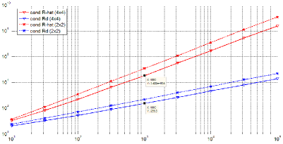
Figure 1: The effect of decomposition of the channel matrix H on the condition number.

IV Hybrid Decoder

Based on the previous findings, a hybrid decoder (HD) can be formed by alternating between the MZF and the ZF decoders based on channel condition number. In particular, the MZF decoder provides performance improvement in case of ill-conditioned channels due to considering only the well conditioned elements of the channel. On the other hand, in case of well-conditioned channels, the ZF decoder can be used without loss of performance. Hence, the hybrid decoder alternates between the traditional ZF decoder and the MZF according to the state of the channel and can be described by the following pseudo-code.

1. Compute the condition number of the channel $cond(H)$.

2. Set a threshold $\gamma$ > 1.

3. If $cond(H)<\gamma$, then $\hat{X}_{ZF}=\lfloor H^{+}y\rceil$.

4. If $cond(H)>\gamma$, then $\hat{X}_{MZF}=\lfloor R_{D}^{-1}Q^{H}y\rceil$.

V Complexity Analysis

The complexity of the proposed algorithm can be measured by computing the number of floating point operations (flops) consumed for execution; which also can be converted into the execution time. It should be noted that $(7)$ is solved using the $QR$ factorization algorithm [7]. So $(7)$ can be re-written as

$$R\hat{X}_{ZF}=Q^{H}y$$ (9)

Which can be solved using back substitution method with cost [7]:

$$flps_{ZF}\approx 2nm^{2}-\frac{2}{3}m^{3}$$ (10)

Similarly, for the MZF decoder,

$$R_{D}\hat{X}_{MZF}=Q^{H}y$$ (11)

The cost of the previous algorithm is the same as the cost of the algorithm of eq. $(10)$ without the cost of back substitution. Where the cost of back substitution is $m^{2}$, the number of flops of MZF algorithm is:

$$flps_{MZF}\approx flps_{ZF}-m^{2}$$ (12)

In HD algorithm; the number of flops is greater than the average between $flps_{ZF}$ and $flps_{MZF}$ by the number of flops consumed in channel condition number calculations.

VI Simulation Results

For comparison purpose, the performance of the proposed decoders ,(MZF) and (HD), are compared to the SD and the ZF for uncoded systems. It is assumed that the transmitted power is independent of the number of transmit antennas, $M$, and equals to the average symbols energy. We have assumed that the channel is Rayleigh fading channel. Let $P$ be the percentage of ill-conditioned channels in the runs. Figures 2, 3, and 4 illustrate the performance of the traditional and proposed decoders for $N=M=2$ ,$16-QAM$ for well-conditioned channels $P=0\%$, ill-conditioned channels with $cond(H)=10^{3}$ for $P=100\%$ and $P=50\%$ versus different values of signal to noise ratio. Figure 5 illustrates the performance for different values of channel condition numbers for $SNR=15dB$. As it is clear from the figures, the SD is superior while the ZF and the MZF decoders are inferior. It should be noted that in the well-conditioned channel case, as illustrated in figure 2, the MZF decoder performance has an error floor. This is a natural byproduct of neglecting of one of the well-conditioned channel component, $\hat{R}$, as expected. Thus, the HD typically follows the ZF because it acts as a ZF in well-conditioned channels, $P=0\%$, as indicated before. Similarly, for the ill-conditioned channels, $P=100$, illustrated in figure 3, the performance of the ZF decoder produces an error floor. This is expected due to the noise enhancement inherent in the ZF decoder [6]. Figure 4 shows that as the percentage of ill-conditioned channels increases, the performance of HD is very close to SD performance especially in low SNR. Also, as shown in figures 5 and 6 the performance of the HD approaches the SD performance with the increase of the channel condition number especially in low SNR as shown in figure 6 .

The complexities of the SD, ZF, MZF, and HD are measured by the execution time in finding the solution. In particular, figures 7 illustrates the complexity for the $2\times 2$ MIMO with $16-QAM$ modulation as a function of the SNR. It is clear that the SD has high complexity while the MZF and the ZF decoders has low complexity. As it is clear from $(12)$, the complexity of MZF decoder is less than the complexity of the ZF decoder by a small margin according.

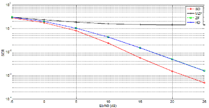
Figure 2: Performance of 2$\times$2 MIMO 16-QAM well-conditioned channels (P = 0%)

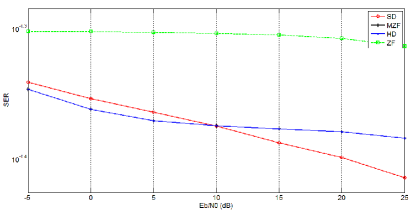
Figure 3: Performance of 2$\times$2 MIMO 16-QAM ill-conditioned channels with cond(H) = $10^{3}$ (P = 100%)

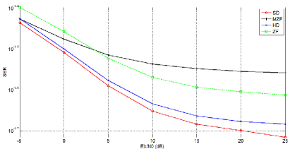
Figure 4: Performance of 2$\times$2 MIMO 16-QAM (P = 50%)

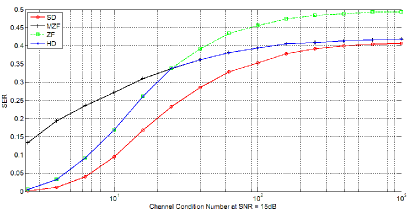
Figure 5: Channel performance varies with a channel condition number for 2$\times$2 MIMO 16-QAM at SNR = 15dB

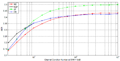
Figure 6: Channel performance varies with a channel condition number for 2$\times$2 MIMO 16-QAM at SNR = 5dB

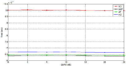
Figure 7: Average Execution Time per Bit for 2$\times$2 MIMO 16-QAM

VII Conclusions

A Hybrid MIMO decoder that is based on neglecting the cross correlation elements of the channel correlation matrix, $R$, in ill-conditioned channels and acting as ZF in well-conditioned channels has been proposed. The proposed decoder has better performance in ill-conditioned channels than the corresponding ZF decoder. The complexity of the proposed decoder is as low as the ZF decoder.

References

- [1] Ramin Shariat-Yazdi and Tad Kwasniewski, “Configurable K-best MIMO Detector Architecture,” ISCCSP 2008, Malta, 12-14 March 2008.
- [2] Chung-An Shen and Ahmed M. Eltawil, “An Adaptive Reduced Com- plexity K-Best Decoding Algorithm with Early Termination,” IEEE CCNC 2010 proceedings.
- [3] Y. Cho et. al, "MIMO-OFDM Wireless Communications with MATLAB", chapter 11, John Wiley & Sons (Asia) Pte Ltd, 2010.
- [4] Yi Hsuan Wu, Yu Ting Liu, Hsiu-Chi Chang, Yen-Chin Liao, and Hsie- Chia Chang, “Early-Pruned K-Best Sphere Decoding Algorithm Based on Radius Constraints,” IEEE Communications Society, ICC 2008.
- [5] N. Sathish Kumar and K. R. Shankar Kumar, “Performance analysis and comparison of m x n zero forcing and MMSE equalizer based receiver for mimo wireless channel,” Songklanakarin J. Sci. Univ. 33 (3), 335-340, May - Jun. 2011.
- [6] Michael T. Heath, “Scientific Computing: An Introductory Survey,” chapter 2, ISBN-10: 0071244891, 2001.
- [7] Lloyd N. Trefethen, David Bau, “Numerical Linear Algebra,” lecture 11, 1997.