(py)LIon: a package for simulating trapped ion trajectories

Abstract

The (py)LIon package is a set of tools to simulate the classical trajectories of ensembles of ions in electrodynamic traps. Molecular dynamics simulations are performed using LAMMPS, an efficient and feature-rich program. (py)LIon has been validated by comparison with the analytic theory describing ion trap dynamics. Notable features include GPU-accelerated force calculations, and treating collections of ions as rigid bodies to enable investigations of the rotational dynamics of large, mesoscopic charged particles.

PROGRAM SUMMARY

Manuscript Title: (py)LIon: a package for simulating trapped ion trajectories
Authors: E. Bentine, C. J. Foot, D. Trypogeorgos
Program Title: (py)LIon
Licensing provisions: MIT
Programming language: Matlab, Python
Computer: pc, cluster
Operating system: Windows, Linux, Mac
RAM: size-dependent
Number of processors used: user-configurable
Keywords: LAMMPS, ion trap, electrodynamic trap, molecular dynamics
Classification: 2 Atomic Physics, 12 Gases and Fluids, 16 Molecular Physics and Physical Chemistry
Subprograms used: LAMMPS
Nature of problem: Simulating the dynamics of ions and mesoscopic charged particles confined in an electrodynamic trap using molecular dynamics methods
Solution method: Provide a tested, feature-rich API to configure molecular dynamics calculations in LAMMPS
Unusual features: (py)LIon can treat collections of ions as rigid bodies to simulate larger objects confined in electrodynamic traps. GPU acceleration is provided through the LAMMPS gpu package.
Running time: Size-dependent, ranges from seconds to hours on a recent workstation.

1 Introduction

Electrodynamic ion traps, also known as Paul traps, are widely used in physics and chemistry to confine charged particles [1]. Their applications include mass spectrometry, quantum chemistry, ultra-high precision frequency measurements, and quantum computation [2, 3, 4, 5]. The dynamics of ions confined in these traps can be simulated using molecular dynamics techniques [6, 7, 8], in which classical equations of motion for the ions are integrated.

Molecular dynamics techniques are also widely used in chemistry to simulate the interactions and properties of macromolecules, membranes, polymers and other systems by computing the trajectories of the constituent atoms. A number of programs have been developed to simulate these systems [9, 10, 11, 12], which typically comprise thousands to millions of atoms and are dominated by short-range forces. These codes are efficient and feature-rich, with numerous accelerated methods for integration and both long- and short-ranged force calculations.

The (py)LIon package is a set of tools to simulate the classical trajectories of ions in electrodynamic traps. The time-integration is performed using LAMMPS, an established classical molecular dynamics code, which is more typically used for biological and materials modelling [9]. (py)LIon offers a robust way to author ion trap simulations, with a simplified workflow that is geared towards the atomic physics community. In addition, the results from (py)LIon have been verified by comparison to analytical descriptions of ion trap dynamics.

Performing simulations in LAMMPS allows (py)LIon to leverage a number of advanced methods, models and features. For instance, calculations can be performed using a graphics processing unit (GPU), which decreases the time taken to calculate the Coulomb repulsion between large numbers of ions [6]. Additionally, (py)LIon supports fixing individual particles together to create rigid bodies. This feature enables the rotational dynamics of trapped ions to be simulated, which is particularly interesting for systems of larger ions [13, 14, 15]. Such investigations are not possible in other ion trap simulation packages, which are restricted to point-like particles.

This paper describes the use and implementation of (py)LIon as follows. In sec:dynamicseq:Eq. (2)sec:dynamicsfig:Figure 2sec:dynamicstab:Table 2sec:dynamicsappendix:Appendix 2sec:dynamicssec:Section 2, we describe the dynamics of charged particles in electrodynamic traps. In sec:overviewpleq:Eq. (3)sec:overviewplfig:Figure 3sec:overviewpltab:Table 3sec:overviewplappendix:Appendix 3sec:overviewplsec:Section 3, we provide an overview of (py)LIon, and describe the features of a typical simulation. In sec:exampleeq:Eq. (4)sec:examplefig:Figure 4sec:exampletab:Table 4sec:exampleappendix:Appendix 4sec:examplesec:Section 4, we walk through example scripts and benchmark the performance of (py)LIon. In sec:Validationeq:Eq. (5)sec:Validationfig:Figure 5sec:Validationtab:Table 5sec:Validationappendix:Appendix 5sec:Validationsec:Section 5, we validate the output of (py)LIon by comparing test simulations to analytic results. In sec:Implementationeq:Eq. (6)sec:Implementationfig:Figure 6sec:Implementationtab:Table 6sec:Implementationappendix:Appendix 6sec:Implementationsec:Section 6, we provide details of (py)LIon’s implementation and discuss the configuration of LAMMPS. We conclude in sec:Conclusioneq:Eq. (7)sec:Conclusionfig:Figure 7sec:Conclusiontab:Table 7sec:Conclusionappendix:Appendix 7sec:Conclusionsec:Section 7, and provide information for getting started in sec:gettingStartedeq:Eq. (8)sec:gettingStartedfig:Figure 8sec:gettingStartedtab:Table 8sec:gettingStartedappendix:Appendix 8sec:gettingStartedsec:Section 8.

(py)LIon is available for both Matlab and Python. The workflow is similar for both languages, and for brevity we describe only the Matlab package in detail here.

2 Dynamics of trapped ions

Electrodynamic traps confine ions using a combination of dc and ac electric fields that exert an oscillating, position-dependent force on a charged particle to circumvent Earnshaw’s theorem and allow trapping [16, 17]. An ion of charge $Q$ and mass $M$ in a linear Paul trap is confined by the quadrupole electric field

$$\mathbf{E}(\mathbf{x},t)=\frac{V_{0}}{R_{0}^{2}}\cos\Omega t\left(x\mathbf{\hat{e}}_{x}-y\mathbf{\hat{e}}_{y}\right)+\frac{\kappa U_{0}}{Z_{0}^{2}}(2z\mathbf{\hat{e}}_{z}-x\mathbf{\hat{e}}_{x}-y\mathbf{\hat{e}}_{y}),$$ (1)

where $V_{0}$, $U_{0}$ are the amplitudes of the ac and dc voltages, $R_{0}$, $Z_{0}$ are characteristic lengths along the radial and axial directions that are related to the distance between the trap electrodes, and $\kappa$ is a geometrical factor [18, 17]. The quantities $\mathbf{\hat{e}}_{i}$ indicate unit vectors along the Cartesian axes. The ion’s motion in each dimension $m$ separates into a rapid ‘micromotion’ at frequency $\Omega$ and a slow oscillation at the secular frequency $\omega_{m}$. The pseudopotential approximation is often used, in which one neglects the micromotion and treats the ion as being trapped in an effective harmonic potential with secular frequency $\omega_{m}/2\pi$, where

$$\omega_{m}\simeq\frac{\Omega}{2}\sqrt{a_{m}+\frac{1}{2}q_{m}^{2}}.$$ (2)

The $a_{m}$ and $q_{m}$ are the Mathieu coefficients, defined as

$$\begin{split}a_{x}&=a_{y}=-\frac{1}{2}a_{z}=-\frac{4Q\kappa U_{0}}{MZ_{0}^{2}\Omega^{2}},\\ q_{x}&=-q_{y}=\frac{2QV_{0}}{MR_{0}^{2}\Omega^{2}},\quad q_{z}=0.\end{split}$$ (3)

The pseudopotential approximation is strictly valid only for $|q_{m}|,\,|a_{m}|\ll 1$, but it remains accurate to 1% up to $q=0.4$.

An ensemble of trapped ions experience both the external trapping fields and a mutual Coulomb interaction. The total potential energy in the pseudopotential approximation is

$$V(\vec{x})=\frac{1}{2}\sum_{i=1}^{N}U_{i}(\vec{x})+\sum_{\begin{subarray}{c}i,j=1\\ i\neq j\end{subarray}}^{N}\frac{1}{8\pi\epsilon_{0}}\frac{Q_{i}Q_{j}}{|\vec{x}_{j}-\vec{x}_{i}|},$$ (4)

where $U_{i}(\vec{x})=M_{i}(\vec{\omega}_{i}^{2}\cdot\vec{x}_{i}^{2})/2$ is the confining potential for ions $i,j$ of mass $M_{i}$, secular frequencies $\vec{\omega}_{i}/2\pi=\{\omega_{x},\omega_{y},\omega_{z}\}/2\pi$ and charge $Q_{i}$. $\epsilon_{0}$ is the permittivity of free space, and $N$ the number of ions. Equation 4 excludes effects such as heating arising from the micromotion of the ions, which require a treatment using the full time-dependent electric field of eq:fieldeq:Eq. (1)eq:fieldfig:Figure 1eq:fieldtab:Table 1eq:fieldappendix:Appendix 1eq:fieldsec:Section 1.

The ground state configuration of the system is an ordered structure called a Coulomb crystal. The system crystallises at sufficiently low temperatures where the kinetic energy of the ions is negligible compared to the trapping potential and the repulsive Coulomb forces, which fix the positions of the ions. This is achieved in practice using methods such as laser cooling or buffer gas cooling to extract kinetic energy from the ion ensemble.

3 Overview of (py)LIon

(py)LIon provides high-level functions to configure and execute simulations of charged particles in ion traps. fig:flowDiagrameq:Eq. (1)fig:flowDiagramfig:Figure 1fig:flowDiagramtab:Table 1fig:flowDiagramappendix:Appendix 1fig:flowDiagramsec:Section 1 shows the process flow of a typical program. (py)LIon translates a configured simulation into an input file and submits it to LAMMPS, which performs the molecular dynamics. Once the simulation is complete, process control reverts to the chosen environment for post-processing and analysis.

The configuration of a typical simulation in (py)LIon proceeds as follows:

1. Create the simulation and specify the domain.

2. Define the atomic species used and create ions.

3. Configure the trap parameters, using either the full electric fields or the pseudopotential approximation.

4. Configure other applied forces, e.g. laser cooling, bias electric fields, Langevin baths.

5. Select which parameters to save, and the periodicity with which to save them.

6. Run the simulation to integrate the equations of motion.

For clarity, commands and syntax in (py)LIon are shown like so.

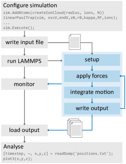
Figure 1: Flow diagram depicting configuration and execution of a LAMMPS simulation using (py)LIon. A simulation is defined through high-level commands in the chosen environment (grey). When the simulation is executed an input file to configure LAMMPS is generated and a LAMMPS child process spawned (blue). An asynchronous loop monitors progress and checks for errors. Time-dependent properties of the simulation are written to output file(s). On completion control reverts back to the main environment for post-processing and analysis.

3.1 Creating the simulation

An instance of the LAMMPSSimulation class represents a simulation, which we refer to by the shorthand sim. High-level (py)LIon commands modify this object, which contains all the information required to generate the LAMMPS input file. The sim object has a few global configuration properties. The NeighbourList style and the CoulombCutoff and NeighbourSkin distances (see sec:pairwiseeq:Eq. (6.3)sec:pairwisefig:Figure 6.3sec:pairwisetab:Table 6.3sec:pairwiseappendix:Appendix 6.3sec:pairwisesec:Section 6.3) configure the pairwise interactions. The GPUAccel switch enables or disables acceleration using a GPU (see sec:GPUeq:Eq. (4.4)sec:GPUfig:Figure 4.4sec:GPUtab:Table 4.4sec:GPUappendix:Appendix 4.4sec:GPUsec:Section 4.4). TimeStep sets the step duration used for time evolution of the system. When unset, (py)LIon attempts to select an appropriate step size by considering the fastest timescale of the simulation, which is typically the period of the oscillating quadrupole field.

3.2 Simulation domain

sim.SetSimulationDomain defines a volume of space within which the ion trajectories are integrated. This must be specified before adding ions or forces to the simulation. (py)LIon will expand the simulation domain during time evolution when required, but the specified domain must contain all ions at the start of the simulation.

3.3 Adding ions

sim.AddAtomType(charge, mass) adds a new atomic species, defined by its charge in units of elementary charge $+e$, and mass in atomic mass units. Once a species is defined, ions can be placed in the simulation. For instance, the command atomCloud(sim, radius, species, N) creates N ions of the desired species randomly placed within the stated radius. For more precise control over the ion positions, such as when defining ions to form a rigid body, placeAtoms(sim, atomType, x, y, z) inserts ions at the coordinates specified by the column vectors x, y, z. Each ion is assigned a unique ID when placed.

Groups of ions can be specified using either the constituent atomic species or the unique IDs of the ions. This allows fields and forces to be applied to specific collections of ions. Setting the Rigid parameter of the group to true fixes the relative positions of ions in the group, so binding them together as a rigid body.

3.4 Forces and fields

3.4.1 Electric fields and confinement

efield(Ex, Ey, Ez) creates a static, uniform electric field of the form $\vec{E}=E_{x}\mathbf{\hat{e}}_{x}+E_{y}\mathbf{\hat{e}}_{y}+E_{z}\mathbf{\hat{e}}_{z}$. Linear Paul traps are defined using linearPT (for full fields) or linearPseudoPT (for the pseudopotential approximation), with a parameterization of the fields as in  eq:fieldeq:Eq. (1)eq:fieldfig:Figure 1eq:fieldtab:Table 1eq:fieldappendix:Appendix 1eq:fieldsec:Section 1. Multi-species simulations that use the pseudopotential approximation must define a separate linearPseudoPT for each charged atomic species because the pseudopotential trap frequencies depend on the specific charge $Q/M$.

3.4.2 Cooling the motion of ions

(py)LIon offers two solutions to simulate cooling: coupling to a Langevin bath, and laser cooling.

langevinBath(T, dampingTime, group) creates a Langevin bath with temperature T in Kelvin and dampingTime equal to the $1/e$ velocity-relaxation time in seconds. The optional argument group allows the bath to be applied to a chosen group, which permits e.g.  species-selective cooling or heating of ions. The bath applies both a damping force to reduce the kinetic energy of the ions and stochastic kicks so that ions thermalise at the temperature of the bath [19].

laserCool(species, gamma) provides an anisotropic cooling mechanism for a particular ion species, by only damping motion parallel to the given direction $\vec{\gamma}$. We model laser cooling as a viscous force $f_{\text{laser}}=-M(\vec{\gamma}\cdot\vec{v})\vec{\gamma}$ along the direction of an applied beam that is proportional to the velocity $\vec{v}$ of each ion [19]. Our implementation does not exert a stochastic force and so the temperature is reduced to zero.

3.5 Minimisation

The energy of a cloud of randomly placed ions comes from a combination of the inter-ion Coulomb repulsion, the potential energy in the trap, and the kinetic energy of the ions. The minimize command uses a modified time-integration method that is well-suited for driving the system to its minimum energy configuration. This method damps the equations of motion to extract energy and also limits the distance that each ion can move in a single time step.

Strong damping generally affects the strength of confinement experienced by ions in a Paul trap [20, 21]. Using minimisation with the full oscillating electric fields of the linearPT command will therefore lead to an incorrect minimum energy configuration, because the damped minimisation algorithm changes the effective harmonic trap frequencies. To avoid this effect, minimisation should only be performed when using the linearPseudoPT confinement, which uses fixed harmonic trap frequencies that are unaffected by the presence of damping.

3.6 Time evolution

evolve(N) advances the simulation by integrating the Newtonian equations of motion for N steps. By interleaving evolve with other commands it is possible to add or remove forces and fields at specific times in the simulation, creating complex sequences where trap parameters are varied in the time-domain. An example of this is given in sec:sympatheticCoolingeq:Eq. (4.2)sec:sympatheticCoolingfig:Figure 4.2sec:sympatheticCoolingtab:Table 4.2sec:sympatheticCoolingappendix:Appendix 4.2sec:sympatheticCoolingsec:Section 4.2.

3.7 Writing/reading data

The dump(filename, variables, steps) command writes time-dependent per-ion variables to the given filename at regular intervals every steps timesteps. The cell array variables contains a mixture of string literals and/or LAMMPSVariables, which are the internal representation of a variable in (py)LIon. The command timeAvg(variables, duration) creates a LAMMPSVariable that represents a time-average of another variable. For example, timeAvg(’vx’, 1/RF) averages the velocity in the $\mathbf{\hat{e}}_{x}$-direction over an rf period.

Literals are a shorthand representation for selecting the properties of ions to be output from the simulation and can be any of the following types:

1. ion coordinates: x, y, z

2. ion velocities: vx, vy, vz

3. the id of each ion

4. time-independent ion properties: mass, charge

The order of ions in the output file may change as they move between processor partitions during the simulation. To enable the reordering of data during postprocessing, the dump command automatically configures output files to include ion ids. These are used by the readDump command to reconstruct trajectories when loading the output file.

3.8 Execution

sim.Execute() runs a configured simulation. (py)LIon generates the LAMMPS input file, launches the LAMMPS executable, and monitors its progress via an asynchronous update loop that handles errors and provides diagnostic information. The process terminates automatically after completion of a simulation, or if the user aborts a (py)LIon simulation. (py)LIon will raise an exception if the sim object is modified after execution. This guarantees that the state of sim remains a faithful description of the executed simulation.

4 Examples

4.1 Coulomb crystal of a single species

We define the electric fields of an ion trap, confine a small cloud of calcium ions, and cool them into a Coulomb crystal by coupling them to a Langevin bath.

⬇

sim = LAMMPSSimulation();

sim.SetSimulationDomain(1e-3,1e-3,1e-3);

caIons = sim.AddAtomType(1, 40);

createIonCloud(sim, 1e-3, caIons, 100, 1);

RF = 3.85e6;

sim.Add(linearPT(300, 7, 2.75e-3, 3.5e-3, 0.3, RF));

T = 1e-3;

sim.Add(langevinBath(T, 10e-6, sim.Group(caIons)));

sim.Add(dump(’pos.txt’, {’id’, ’x’, ’y’, ’z’}, 1));

secularVel = timeAvg({’vx’, ’vy’, ’vz’}, 1/RF);

sim.Add(dump(’secV.txt’, {’id’, secularVel}));

sim.Add(evolve(20000));

sim.Execute();

First, we create the LAMMPSSimulation instance that will represent the simulation and configure a $$1\text{\,}\mathrm{mm}$\times$1\text{\,}\mathrm{mm}$\times$1\text{\,}\mathrm{mm}$$ initial simulation domain for the ions. We define the ${}^{40}\text{Ca}^{+}$ species with $M=$40\text{\,}\mathrm{a}\mathrm{m}\mathrm{u}$$ and charge $Q=$1\text{\,}\mathrm{e}$$. A cloud of 100 randomly-placed ions is added to the simulation domain with createIonCloud. We add a linear Paul trap with an oscillating voltage of $300\text{\,}\mathrm{V}$, endcap voltage of $7\text{\,}\mathrm{V}$, $r_{0}=$2.75\text{\,}\mathrm{mm}$$, $z_{0}=$3.5\text{\,}\mathrm{mm}$$, geometric constant $\kappa=0.3$ and frequency $\Omega/2\pi=$3.85\text{\,}\mathrm{MHz}$$.

To cool the translational motion of the ions, we couple them to a Langevin bath that damps the velocity of the ions with a relaxation time of $10\text{\,}\mathrm{\SIUnitSymbolMicro s}$, and also delivers a small random kick to each ion every time-step such that the temperature of the ensemble relaxes to $1\text{\,}\mathrm{mK}$.

We configure sim to output data using dump. In this example we output the positions of ions every timestep and time-averaged secular velocities every period of the oscillating field, $2\pi/\Omega$. The command evolve instructs the simulation to integrate for 20000 steps. Finally, the configured sim is executed, which writes the input file, launches the LAMMPS process and runs the simulation. The resulting trajectories and equilibrium positions are shown in Figure 2.

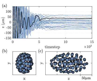
Figure 2: The formation of a 100-ion Coulomb crystal. Ions start from random positions at a high temperature. A structure forms as their motion is cooled by the action of the Langevin bath over many time-steps. (a) Time evolution of the positions of ions along $\mathbf{\hat{e}}_{z}$, showing a gaseous phase of random, changing positions that transitions to an ordered structure. For clarity, only 30 ions are shown, and one trajectory is highlighted in black. (b) & (c) Front and side views of the final positions of ions, illustrating the ordered Coulomb crystal structure. The shading indicates distance from the camera, with ions that are further away rendered in darker colours.

4.2 Sympathetic cooling

(py)LIon supports multiple ion species and the application of species-selective forces. In this example we model the sympathetic cooling of $\text{NH}_{3}^{+}$ ions by laser-cooled calcium ions [23, 24].

⬇

sim = LAMMPSSimulation();

sim.GPUAccel = 1;

SetSimulationDomain(sim, 1e-3,1e-3,1e-3);

NH3 = AddAtomType(sim, 1, 17);

Ca40 = AddAtomType(sim, 1, 40);

createIonCloud(sim, 5e-4, NH3, 20);

createIonCloud(sim, 5e-4, Ca40, 50);

rf = 5.634e6;

sim.Add(linearPT(252.2, 5, 10e-3, 3.5e-3, 0.3, rf));

allBath = langevinBath(1e-3, 30e-6);

sim.Add(allBath);

sim.Add(evolve(100000));

sim.Add(dump(’output.txt’, {’id’, ’x’, ’y’, ’z’, timeAvg({’vx’, ’vy’, ’vz’}, 1/rf)}, 20));

sim.Add(evolve(60000));

sim.Remove(allBath);

sim.Add(laserCool(Ca40, [1e5 0 0]));

sim.Add(evolve(120000));

sim.Execute();

We start by defining the sim object and this time we set GPUAccel to enable GPU acceleration. We create the two ion clouds, define the Paul trap parameters as before, and couple both species to a Langevin bath at $1\text{\,}\mathrm{mK}$. The first evolve brings both species to thermal equilibrium with the bath. At this time $t_{\text{cool}}$ we remove the bath with sim.Remove, add laser-cooling along the $\hat{x}$-axis to the ${}^{40}\text{Ca}^{+}$ ions, and evolve the system again.

fig:example2eq:Eq. (3)fig:example2fig:Figure 3fig:example2tab:Table 3fig:example2appendix:Appendix 3fig:example2sec:Section 3 shows the final equilibrium positions and the kinetic energy of both species. The lighter $\text{NH}_{3}^{+}$ ions are confined tightly in the centre of the trap while the heavier ${}^{40}\text{Ca}^{+}$ ions form a sheath around them. The energy of both species is damped over time; it takes longer for the $\text{NH}_{3}^{+}$ ions to reach the equilibrium temperature since they are only indirectly cooled via interactions with the cloud of laser-cooled ${}^{40}\text{Ca}^{+}$ ions.

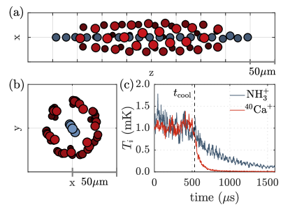
Figure 3: A dual-species simulation of 20 $\text{NH}_{3}^{+}$ ions and 50 ${}^{40}\text{Ca}^{+}$ ions in a linear Paul trap, seen (a) from the side and (b) along the axis of the trap. The $\text{NH}_{3}^{+}$ ions (blue) are confined tightly to the axis of the trap, while the lower charge-to-mass ratio ${}^{40}\text{Ca}^{+}$ ions (red) form a sheath that surrounds them. c) At $t_{\text{cool}}$ (black, dashed line) a $1\text{\,}\mathrm{mK}$ Langevin bath is removed and laser cooling is applied to the $\hat{x}$-axis motion of the ${}^{40}\text{Ca}^{+}$ ions. The temperature of the ${}^{40}\text{Ca}^{+}$ ensemble is cooled quickly, while the interaction between the species causes sympathetic cooling of the $\text{NH}_{3}^{+}$ ions at a slower rate.

4.3 Charged rigid body

This example simulates a group of ions which are bound together to create a rigid body. This body then interacts with a cloud of ions.

⬇

sim = LAMMPSSimulation();

sim.SetSimulationDomain(1e-3,1e-3,1e-3);

mass = 40; charge = 1;

Ca = sim.AddAtomType(charge, mass);

createIonCloud(sim, 1e-4, Ca, 30);

rodz = (-2:0.5:2) * 5e-6;

rody = zeros(size(rodz));

rodx = zeros(size(rodz));

rodAtoms = placeAtoms(sim, Ca, rodx’, rody’, rodz’);

rod = sim.Group(rodAtoms);

rod.Rigid = true;

RF = 3.85e6;

sim.Add(linearPT(500, 15, 2.75e-3, 3.5e-3, 0.3, RF));

sim.Add(langevinBath(0, 1e-5));

sim.Add(dump(’pos.txt’, {’id’, ’x’, ’y’, ’z’}, 2));

secularVel = timeAvg({’vx’, ’vy’, ’vz’}, 1/RF)

sim.Add(dump(’secV.txt’, {’id’, secularVel}));

sim.Add(evolve(5000));

sim.Execute();

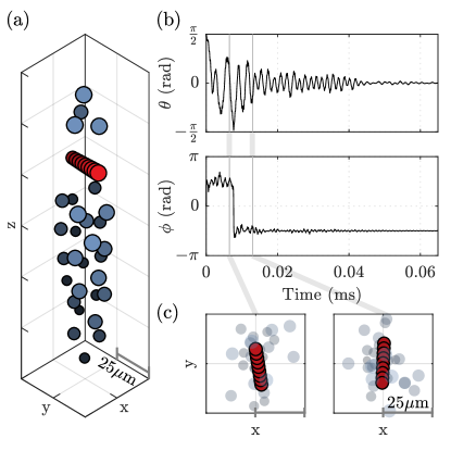
Figure 4: A cloud of ${}^{40}\text{Ca}^{+}$ ions and a rigid rod, which is composed of 9 ions fixed together. After cooling via coupling to a Langevin bath, the ions and rod arrange into a Coulomb crystal. (a) The final positions of ions in the cloud (blue) and the rod (red). (b) The polar angles $\theta(t)$ and $\phi(t)$ describe the orientation of the rod. These quantities are plotted against time $t$, showing that the rod initially tumbles before aligning with respect to the trap and other ions and performing a small thermal motion. (c) Two panels showing a top view of ion positions at early times in the simulation, before the Coulomb crystal has formed. The plot shows the free ions as transparent so that the rod is clearly visible. The specific times shown are illustrated by the vertical lines in panel b.

We start as before, configuring a simulation with two sets of calcium ions. The first are placed randomly, while the second set of ions are arranged in a line and grouped together, forming a rod. Setting the Rigid property of the group to true fixes the relative positions of ions. The system is coupled to a zero temperature bath and forms a Coulomb crystal after time evolution. fig:rigidbodyeq:Eq. (4)fig:rigidbodyfig:Figure 4fig:rigidbodytab:Table 4fig:rigidbodyappendix:Appendix 4fig:rigidbodysec:Section 4 shows the results of the simulation. Ions in the rod form a rigid body, which moves and rotates according to the forces applied to the constituent ions.

4.4 Benchmarking

Our benchmark simulations are performed for different numbers of ions $N$ and using two standard workstations: a Dell Optiplex 9020 with an i7-4790 4-core CPU at $3.6\text{\,}\mathrm{GHz}$ and 8 GB of RAM, and a Lenovo ThinkCentre M900 with an i7-6700 4-core CPU at $3.4\text{\,}\mathrm{GHz}$ and 24 GB of RAM. In addition, the Lenovo is fitted with an nVidia Titan XP GPU, which has 12 GB of GDDR5 RAM and a processor frequency of $1.5\text{\,}\mathrm{GHz}$.

The computation time in the CPU-only simulations begins to scale as $N^{2}$ above $N\approx 30$ ions, where it becomes dominated by calculation of the long-ranged Coulomb repulsion. The brute-force method used involves looping over interacting pairs, the total number of which is proportional to $N^{2}$. For $N<30$ the step computation time is independent of ion number, indicating that an overhead in the LAMMPS integration loop limits the speed of the calculation.

Setting sim.GPUAccel to true enables GPU acceleration. This reduces the calculation time for pairwise interactions between large numbers of ions, and becomes advantageous when simulating more than a few hundred ions (see fig:benchmarkingeq:Eq. (5)fig:benchmarkingfig:Figure 5fig:benchmarkingtab:Table 5fig:benchmarkingappendix:Appendix 5fig:benchmarkingsec:Section 5). GPU Acceleration corresponds to an order-of-magnitude improvement in time for $N\approx 1000$. For $N<300$, GPU acceleration becomes inefficient because of the overhead required to configure tasks on the GPU.

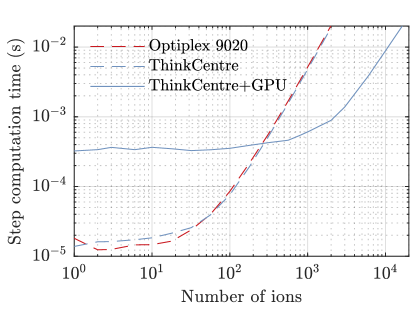
Figure 5: Average computation time per timestep in the benchmark simulations, as a function of ion number. Dashed lines denote CPU-only simulations, solid lines show simulations that are accelerated by the GPU. See text for discussion and a description of the two workstations used.

5 Verifications

(py)LIon is distributed with a test suite which verifies functionality by comparing generated output to analytic results. These validations provide a means to detect if modifications introduce errors, ensuring the integrity of (py)LIon during further development. This section describes each test simulation, the expected behaviour, and the functionality tested.

5.1 Secular motion frequencies

SecularFrequencies_pseudoPot.m and _fullRF.m test the (py)LIon implementation of the linear Paul trap, using either the pseudopotential approximation or the full electric fields respectively. These verifications configure a linear Paul trap, simulate the motion of a single ion and compare the single ion oscillation frequencies to those predicted by eq. (2) (see fig:ver1eq:Eq. (6)fig:ver1fig:Figure 6fig:ver1tab:Table 6fig:ver1appendix:Appendix 6fig:ver1sec:Section 6). We take the measured oscillation frequency along each axis to be the Fourier component with the largest amplitude.

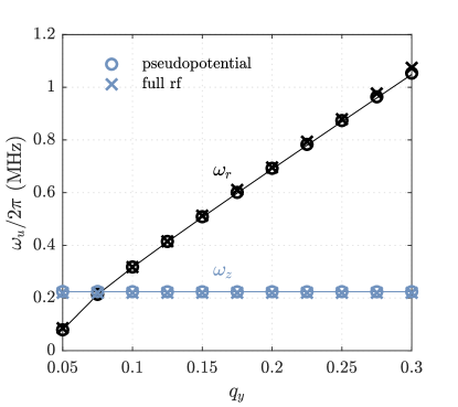
Figure 6: Secular frequencies $\omega_{u}/2\pi$ measured from simulations of a single ion in a linear Paul trap. Those in the radial direction (black) and along $\mathbf{\hat{e}}_{z}$ (blue) are compared to theory (solid lines), for simulations using either the pseudopotential (circles) or full electric fields (crosses).

5.2 Equilibrium separation

The lowest energy configuration when $\omega_{x,y}\gg\omega_{z}$ is a linear Coulomb crystal of $N$ ions aligned along the axis $\hat{e}_{z}$. The position of the $i$th ion, $z_{i}$, depends on the interplay between the confinement along the $\hat{e}_{z}$-axis, which compresses the chain, and the Coulomb repulsion from the other ions. These positions may be found by minimising the potential energy of eq:fullPotentialeq:Eq. (4)eq:fullPotentialfig:Figure 4eq:fullPotentialtab:Table 4eq:fullPotentialappendix:Appendix 4eq:fullPotentialsec:Section 4. The separation between neighbouring ions increases away from the centre of the chain, where the minimum separation is approximately [25]

$$\frac{z_{\mathrm{min}}}{l}=\frac{2.018}{N^{0.559}},\quad\text{with}\ l^{3}=\frac{Q^{2}}{4\pi\epsilon_{0}M\omega_{z}^{2}}.$$ (5)

AxialSeparation.m minimises the energy of ions arranged in a linear Coulomb crystal, and compares the simulated positions $z_{i}$ to those predicted by theory [25] (see fig:ver_equilPoseq:Eq. (7)fig:ver_equilPosfig:Figure 7fig:ver_equilPostab:Table 7fig:ver_equilPosappendix:Appendix 7fig:ver_equilPossec:Section 7). Simulations of these equilibrium positions test the implementations of both the Coulomb interaction and the axial confinement strength of the Paul trap.

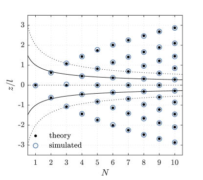
Figure 7: Normalised equilibrium positions $z/l$ of $N$ ions in a linear chain. There is good agreement between theoretical predictions (black dots) and simulation results (blue circles) performed using the pseudopotential approximation. For even $N>1$, the two neighbouring ions that are closest are those at $z=\pm z_{\mathrm{min}}/2$ (solid black lines). For odd $N>1$, they are the pairs positioned at $z=0$ and $z=\pm z_{\mathrm{min}}$ (dotted black lines).

5.3 Normal modes of motion

NormalModes_Linear.m simulates the normal mode spectrum for a fixed number of ions in a Coulomb crystal. First it drives the system to its lowest energy configuration, then allows it to evolve without any damping using the pseudopotential approximation. The normal modes are excited by delivering a periodic kick to the ensemble, which is implemented by randomising the velocities of the ions. The kicks are broadband enough to excite all the normal modes in the Coulomb crystal, and are sufficiently small in amplitude that the crystal does not ‘melt’. The positions of the ions are written to a file twice for every rf cycle, so that all the modes are visible in the final spectrum, and the amplitudes of these modes are calculated by Fourier transforming the trajectories.

The frequencies of the normal modes for a chain of $N$ ions are the eigenvalues of the Hessian matrix [26] constructed from the spatial derivatives of eq:fullPotentialeq:Eq. (4)eq:fullPotentialfig:Figure 4eq:fullPotentialtab:Table 4eq:fullPotentialappendix:Appendix 4eq:fullPotentialsec:Section 4. For small numbers of ions ($N<7$) the theoretical values are tabulated in Ref. [25]. fig:ver_normalModes_lineareq:Eq. (8)fig:ver_normalModes_linearfig:Figure 8fig:ver_normalModes_lineartab:Table 8fig:ver_normalModes_linearappendix:Appendix 8fig:ver_normalModes_linearsec:Section 8 shows that the theoretical normal modes are in agreement with those calculated by (py)LIon.

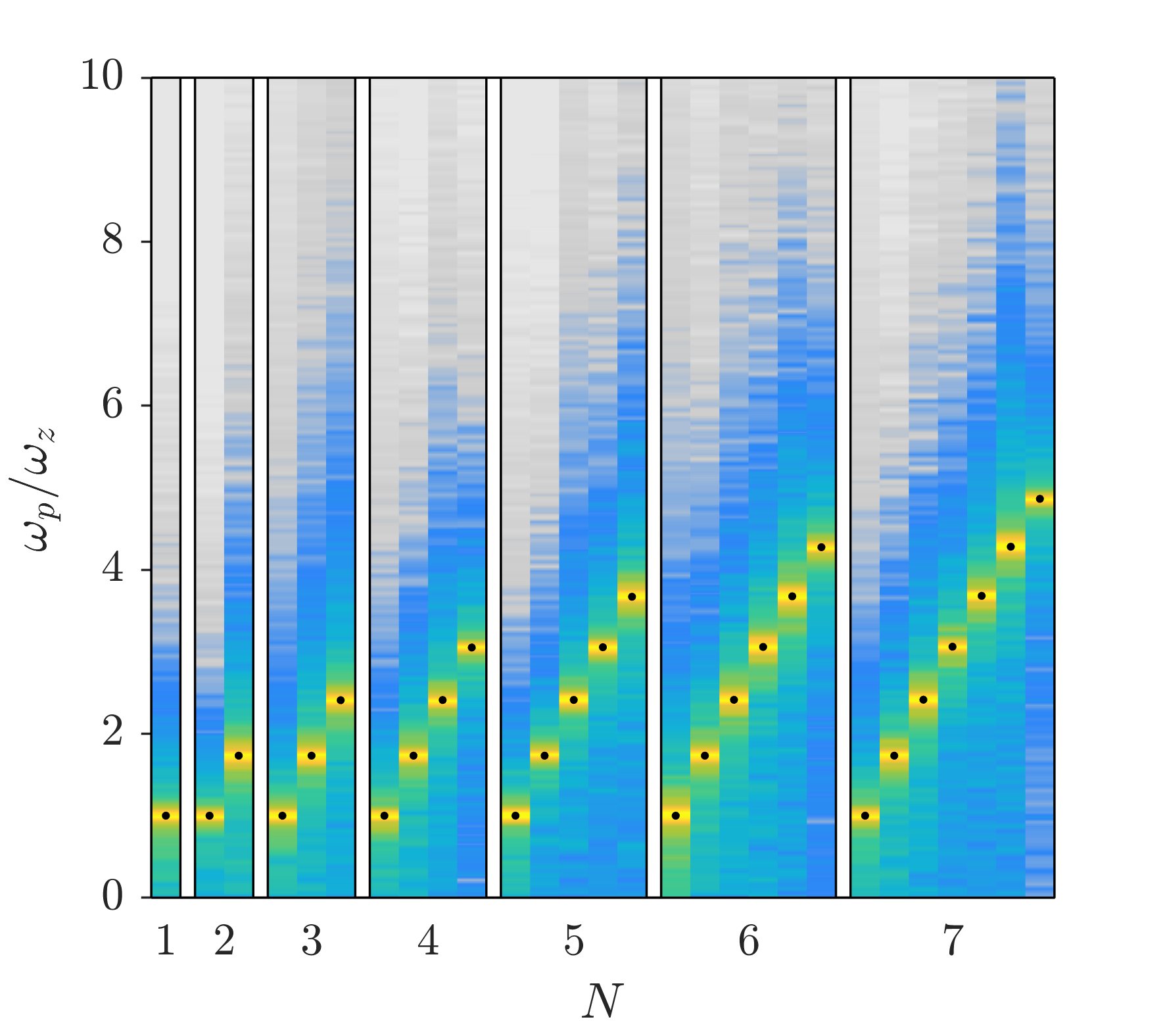
Figure 8: The spectral decomposition of each axial normal mode is shown for simulations of $N$-ion linear Coulomb crystals, where $N\in\{1,7\}$. The vertical axis denotes frequency, normalised with respect to $\omega_{z}$. The frequency spectrum for each normal mode is shown as a vertical colored stripe; the logarithm of intensities are plotted using a colour map where yellow depicts a maximum and grey depicts vanishing amplitude. The maximum amplitude of each mode is in agreement with the predicted frequency of that normal mode (black dot).

5.4 Cooling mechanisms

LaserCooling.m simulates the trajectories of free, non-interacting ions that are strongly laser-cooled along a single randomly-chosen direction, with a characteristic damping time $\tau=$1\text{\,}\mathrm{\SIUnitSymbolMicro}\mathrm{s}$$. It then projects the velocity of each ion onto the laser-cooling axis, fits them with an exponential function and compares the result of the fit to $\tau$. The perpendicular velocity components are unaffected by the laser-cooling force.

LangevinBath.m simulates groups of free, non-interacting atoms. Each group $j$ is coupled to a distinct Langevin bath with time constant $c_{j}$ and temperature $\Phi_{j}$. The equipartition theorem relates the temperature $T_{j}$ of each group to its kinetic energy, $3k_{B}T_{j}=M\langle v_{x}^{2}+v_{y}^{2}+v_{z}^{2}\rangle$, where $k_{B}$ is the Boltzmann constant. fig:ver_langevineq:Eq. (9)fig:ver_langevinfig:Figure 9fig:ver_langevintab:Table 9fig:ver_langevinappendix:Appendix 9fig:ver_langevinsec:Section 9 shows $T_{j}$ for each group as a function of time, along with theoretical curves (no fit) showing the predicted temperature as each ensemble thermalizes with the associated bath in accordance with Newton’s law of cooling.

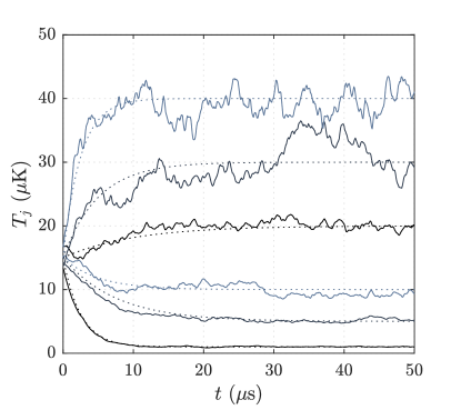
Figure 9: Groups of free, non-interacting atoms are each coupled to a different Langevin bath and the dynamics simulated. Measured temperatures $T_{j}$ of each group are shown as solid lines, while dotted lines show the predicted temperature of that group, given the known coupling strength and temperature $\Phi_{j}$ of the associated bath.

6 Implementation Details

Having described the usage and validity of our package, we now address its implementation. Although an understanding of LAMMPS is not required to use (py)LIon, in this section we provide pertinent details of the LAMMPS configuration and features used, which are useful for implementing new features. For clarity, the commands specific to LAMMPS are indicated like so.

6.1 Input file preamble

The input file starts with a declaration of the static properties of the simulation. All quantities are defined in terms of SI units using units si. The package gpu and suffix gpu commands toggle GPU acceleration on/off by overriding fix styles in LAMMPS with equivalent GPU implementations [27, 28, 29]. The boundary, region and create_box commands define a non-periodic simulation region.

6.2 Ions in LAMMPS

The LAMMPS atom_style charge command configures the simulation to represent ions as atoms with a velocity, position, id and atom type. The create_atoms command adds atoms one-by-one to the input file, placing a single atom of specified type and position each time. The mass and set type commands subsequently configure the different atom types.

6.3 Interactions

To determine which atoms should interact through pairwise potentials, LAMMPS creates neighbour lists of atoms within a threshold distance of each other. The threshold is equal to the force cut-off distance plus a skin distance which for greater values reduces the frequency at which the list becomes invalid and must be rebuilt. This approach is computationally efficient for systems of short-ranged forces in which atoms frequently aquire new neighbours, but is redundant for systems of ions because each ion interacts with all other ions for the duration of the simulation. As such, (py)LIon configures LAMMPS to build the neighbour list once at the start of the simulation using the nsq style, and with all ions listed as neighbours.

The pair_style command specifies the interaction model used between neighbouring atoms. (py)LIon disables short-ranged interactions such as Van der Waals forces because the spatial separation between ions is typically orders of magnitude larger than the length scales of these forces. The pair style coul/cut defines a truncated Coulomb interaction. The default cut-off distance is chosen to be $10\text{\,}\mathrm{m}$, which makes it effectively infinite for typical-size systems.

The pairwise interaction represents the most computationally intense part of the integration. A brute force method that directly sums these forces scales as $\mathcal{O}(N^{2})$, which becomes unfavourable for large particle numbers, but is well-suited to parallel computation. Other methods for calculating long-ranged forces are implemented in LAMMPS, such as multi-level summation [30]. Ewald summation and particle-particle/particle-mesh methods are also available for systems with periodic boundary conditions [28], although these are not suited to ion traps. We have found that (py)LIon performs well using the brute-force summation method for our typical simulation sizes of 100 atoms (see sec:GPUeq:Eq. (4.4)sec:GPUfig:Figure 4.4sec:GPUtab:Table 4.4sec:GPUappendix:Appendix 4.4sec:GPUsec:Section 4.4), and so have not exposed these other methods to (py)LIon.

6.4 Simulation elements

The remainder of the input file describes successive definitions of forces, variables, output, and evolution. These are each contained in the ordered array sim.Elements as InputFileElements. (py)LIon enumerates the array, generating the required input file content by invoking each element’s createInputFileText function. This is also the mechanism by which (py)LIon can be extended; the extension only needs to implement the createInputFileText method to return the appropriate input file text required to configure the targeted LAMMPS feature. For instance, a (py)LIon efield element inserts the text fix <fixID> all efield <Ex> <Ey> <Ez> to the input file, using a unique identifier <fixID> for the force and specifying the components of the electric field.

6.5 Integration

The nve integrator updates the positions of single atoms at each integration step according to the Newtonian equations of motion. We work in the NVE ensemble in which the system is isolated and the total number of ions is conserved. The rigid integrator calculates the motion of rigid bodies, maintaining the relative position of their constituent atoms. timestep defines the fixed step duration used for time integration. (py)LIon configures LAMMPS to print diagnostic information about compute resource usage every 10000 steps using the thermo command.

To minimise the energy of an ensemble the minimize and min_style quickmin commands offer alternative integration schemes that converge in a smaller number of steps (see sec:Minimisationeq:Eq. (3.5)sec:Minimisationfig:Figure 3.5sec:Minimisationtab:Table 3.5sec:Minimisationappendix:Appendix 3.5sec:Minimisationsec:Section 3.5).

7 Conclusion

(py)LIon allows full configuration and execution of ion trap simulations from within a Matlab or Python environment. It offloads the computationally intensive part to LAMMPS, while the environment of choice is used for configuration and analysis. No knowledge of LAMMPS’ specialist command language is required.

Molecular dynamics codes such as LAMMPS are typically associated with calculation of short-range inter-atomic forces that drive mesoscopic material and biophysical processes. We have shown that LAMMPS can also efficiently model systems where long range interactions are dominant, such as electrodynamically confined clouds of ions. Wrapping LAMMPS brings a number of features to (py)LIon, e.g. support for rigidly bound clusters of ions, and GPU acceleration. (py)LIon complements LAMMPS by providing high-level specialised functions that simplify the description of the ion trap system.

All functionality of (py)LIon has been verified by a thorough comparison to theory. We have used (py)LIon to simulate a range of single/multiple species and multi-frequency systems [31, 32]. LAMMPS is a mature code with many other features that can be implemented in (py)LIon. These include electric fields defined by finite element methods (using the atc package), and ion-neutral interactions using direct-simulation Monte Carlo methods. These future extensions will allow (py)LIon to deal with even more complex scenarios, such as: the cooling of large, levitated objects via interaction with a buffer gas or feedback [33]; rarefied gas dynamics to simulate ion collisions with a buffer gas [34]; coarse-grained molecular dynamics simulations of protein structures in aqueous Paul traps [35, 36]; studies of cold molecule production/reactions [37]; and interactions of ions with polar molecules [38].

8 Getting Started

Up-to-date stable releases of LAMMPS are available at http://lammps.sandia.gov/. Multiple build options for LAMMPS exist. At least the misc package must be included, and optionally the rigid and gpu packages for rigid-body and GPU support respectively. The most recent version of (py)LIon’s MATLAB distribution is available at bitbucket.org/footgroup/lion.git, and further documentation and examples can be found in the source. For instructions to install and configure (py)LIon, please see the readme file. The Python version of (py)LIon can be downloaded from bitbucket.org/dtrypogeorgos/pylion, along with documentation explaining how to get started.

References

- [1] W. Paul, Electromagnetic traps for charged and neutral particles, Rev. Mod. Phys. 62 (1990) 531–540. doi:10.1103/RevModPhys.62.531.
- [2] Quadrupole Ion Trap Mass Spectrometry, Volume 165, Second Edition, Wiley-VCH.
- [3] G. C. Stafford, P. E. Kelley, J. E. P. Syka, W. E. Reynolds, J. F. J. Todd, Recent improvements in and analytical applications of advanced ion trap technology 60 (1) 85–98. doi:10.1016/0168-1176(84)80077-4.
- [4] Ion Traps, International Series of Monographs on Physics, Oxford University Press.
- [5] J. Benhelm, G. Kirchmair, C. F. Roos, R. Blatt, Towards fault-tolerant quantum computing with trapped ions 4 (6) 463–466. doi:10.1038/nphys961.
- [6] S. Van Gorp, M. Beck, M. Breitenfeldt, V. De Leebeeck, P. Friedag, A. Herlert, T. Iitaka, J. Mader, V. Kozlov, S. Roccia, G. Soti, M. Tandecki, E. Traykov, F. Wauters, C. Weinheimer, D. Zákoucký, N. Severijns, Simbuca, using a graphics card to simulate Coulomb interactions in a penning trap 638 (1) 192–200. doi:10.1016/j.nima.2010.11.032.
- [7] D. A. Dahl, J. E. Delmore, A. D. Appelhans, SIMION PC/PS2 electrostatic lens design program 61 (1) 607–609. doi:10.1063/1.1141932.
- [8] S. Schiller, C. Lammerzahl, Molecular dynamics simulation of sympathetic crystallization of molecular ions 68 (5) 053406. doi:10.1103/PhysRevA.68.053406.
- [9] C. Trott, L. Winterfeld, General purpose Molecular Dynamics Simulations on GPUs: Issues of Pair Forces and Scaling to large ClustersarXiv:1009.4330.
- [10] T. Matthey, T. Cickovski, S. Hampton, A. Ko, Q. Ma, PROTOMOL, an Object-Oriented Framework for Prototyping Novel Algorithms for Molecular Dynamics, in: In Computational Science—ICCS 2003, International Conference, and St.
- [11] J. C. Phillips, R. Braun, W. Wang, J. Gumbart, E. Tajkhorshid, E. Villa, C. Chipot, R. D. Skeel, L. Kalé, K. Schulten, Scalable molecular dynamics with namd, Journal of Computational Chemistry 26 (16) 1781–1802. arXiv:https://onlinelibrary.wiley.com/doi/pdf/10.1002/jcc.20289, doi:10.1002/jcc.20289.
- [12] H. Berendsen, D. van der Spoel, R. van Drunen, GROMACS: A message-passing parallel molecular dynamics implementation, Computer Physics Communications 91 (1) (1995) 43 – 56. doi:https://doi.org/10.1016/0010-4655(95)00042-E.
- [13] E. Hesse, Z. Ulanowski, P. Kaye, Stability characteristics of cylindrical fibres in an electrodynamic balance designed for single particle investigation, Journal of Aerosol Science 33. doi:10.1016/S0021-8502(01)00153-7.
- [14] B. E. Kane, Levitated spinning graphene flakes in an electric quadrupole ion trap 82 (11) 115441. doi:10.1103/PhysRevB.82.115441.
- [15] T. Delord, L. Nicolas, Y. Chassagneux, G. Hétet, Strong coupling between a single nitrogen-vacancy spin and the rotational mode of diamonds levitating in an ion trap, Phys. Rev. A 96 (6) (2017) 063810. arXiv:1702.00774, doi:10.1103/PhysRevA.96.063810.
- [16] C. J. Foot, Atomic Physics, OUP Oxford.
- [17] D. J. Berkeland, J. D. Miller, J. C. Bergquist, W. M. Itano, D. J. Wineland, Minimization of ion micromotion in a Paul trap 83 (10) 5025–5033. doi:10.1063/1.367318.
- [18] S. Willitsch, M. T. Bell, A. D. Gingell, T. P. Softley, Chemical applications of laser- and sympathetically-cooled ions in ion traps 10 (48) 7200–7210. doi:10.1039/B813408C.
- [19] C. B. Zhang, D. Offenberg, B. Roth, M. A. Wilson, S. Schiller, Molecular-dynamics simulations of cold single-species and multispecies ion ensembles in a linear Paul trap 76 (1) 012719. doi:10.1103/PhysRevA.76.012719.
- [20] M. Nasse, C. Foot, Influence of background pressure on the stability region of a Paul trap 22 563–573. doi:10.1088/0143-0807/22/6/301.
- [21] T. Hasegawa, K. Uehara, Dynamics of a single particle in a Paul trap in the presence of the damping force 61 159–163. doi:10.1007/BF01090937.
- [22] LAMMPS user manual, https://lammps.sandia.gov/doc/Manual.html, accessed: 2019-05-29.
- [23] K. Okada, M. Wada, T. Takayanagi, S. Ohtani, H. A. Schuessler, Characterization of ion coulomb crystals in a linear paul trap, Phys. Rev. A 81 (2010) 013420. doi:10.1103/PhysRevA.81.013420.
- [24] A. Ostendorf, C. B. Zhang, M. A. Wilson, D. Offenberg, B. Roth, S. Schiller, Sympathetic cooling of complex molecular ions to millikelvin temperatures, Phys. Rev. Lett. 97 (2006) 243005. doi:10.1103/PhysRevLett.97.243005.
- [25] D. James, Quantum dynamics of cold trapped ions with application to quantum computation, Applied Physics B 66 (2) (1998) 181–190. doi:10.1007/s003400050373.
- [26] D. Kielpinski, B. E. King, C. J. Myatt, C. A. Sackett, Q. A. Turchette, W. M. Itano, C. Monroe, D. J. Wineland, W. H. Zurek, Sympathetic cooling of trapped ions for quantum logic 61 (3) 032310. doi:10.1103/PhysRevA.61.032310.
- [27] S. J. P. A. N. T. W. M. Brown, P. Wang, Implementing molecular dynamics on hybrid high performance computers - short range forces, Comp. Phys. Comm. 182 (2011) 898–911.
- [28] W. M. Brown, A. Kohlmeyer, S. J. Plimpton, A. N. Tharrington, Implementing molecular dynamics on hybrid high performance computers – particle–particle particle-mesh, Computer Physics Communications 183 (3) (2012) 449 – 459. doi:https://doi.org/10.1016/j.cpc.2011.10.012.
- [29] Y. M. W. M. Brown, Implementing molecular dynamics on hybrid high performance computers – three-body potentials, Comp. Phys. Comm. 184 (2013) 2785–2793.
- [30] D. J. Hardy, J. E. Stone, K. Schulten, Multilevel summation of electrostatic potentials using graphics processing units, Parallel Computing 35 (3) (2009) 164 – 177, revolutionary Technologies for Acceleration of Emerging Petascale Applications. doi:https://doi.org/10.1016/j.parco.2008.12.005.
- [31] C. J. Foot, D. Trypogeorgos, E. Bentine, A. Gardner, M. Keller, Two-frequency operation of a Paul trap to optimise confinement of two species of ions 430 117–125. doi:10.1016/j.ijms.2018.05.007.
- [32] D. Trypogeorgos, C. J. Foot, Cotrapping different species in ion traps using multiple radio frequencies 94 (2) 023609. doi:10.1103/PhysRevA.94.023609.
- [33] P. Nagornykh, B. E. Kane, Parametric stabilization and cooling of microparticles in a quadrupole ion trap, in: Optical Trapping and Optical Micromanipulation XI, Vol. 9164, International Society for Optics and Photonics, p. 916405. doi:10.1117/12.2064969.
- [34] G. A. Bird, Molecular Gas Dynamics and the Direct Simulation of Gas Flows, 2nd Edition, Oxford University Press, USA.
- [35] W. Guan, S. Joseph, J. H. Park, P. S. Krstic, M. A. Reed, Paul trapping of charged particles in aqueous solution 108 (23) 9326–9330. arXiv:21606331, doi:10.1073/pnas.1100977108.
- [36] S. Joseph, W. Guan, M. A. Reed, P. S. Krstic, Long DNA segment in a linear nanoscale Paul trap 21 (1) 015103. arXiv:19946172, doi:10.1088/0957-4484/21/1/015103.
- [37] M. T. Bell, T. P. Softley, Ultracold molecules and ultracold chemistry 107 (2) 99–132. doi:10.1080/00268970902724955.
- [38] Z. Idziaszek, T. Calarco, P. Zoller, Ion-assisted ground-state cooling of a trapped polar molecule 83 (5) 053413. doi:10.1103/PhysRevA.83.053413.