Non-real eigenvalues of the Harmonic Oscillator perturbed by an odd, two-point $\delta$-potential

Abstract.

In this paper, we consider the perturbations of the Harmonic Oscillator Operator by an odd pair of point interactions: $z(\delta\left(x-b\right)-\delta\left(x+b\right))$. We study the spectrum by analyzing a convenient formula for the eigenvalue. We conclude that if $z=ir$, $r$ real, as $r\to\infty$, the number of non-real eigenvalues tends to infinity.

1. Introduction

1.1. Perturbations of the Harmonic Oscillator

We consider the harmonic oscillator operator,

(1.1a) $$\displaystyle L_{\text{HO}}^{0}y(x) \displaystyle=-y^{\prime\prime}(x)+x^{2}y(x),$$

(1.1b) $$\displaystyle\operatorname{\mathfrak{D}}\left(L_{\text{HO}}^{0}\right) \displaystyle\equiv\{y(x)\in\mathcal{H}^{2}(\mathbb{R}):x^{2}y(x)\in L^{2}(\mathbb{R})\}.$$

($\displaystyle\mathcal{H}^{k}(\mathbb{R})=\mathcal{W}^{k,2}(\mathbb{R})$ is a Sobolev space, and we allow $\displaystyle y^{\prime\prime}$ to be a distributional derivative.) The operator is of compact resolvent, and the spectrum is the positive odd integers:

$$\operatorname{Sp}(L_{\text{HO}}^{0})=2\mathbb{N}_{0}+1,\quad\mathbb{N}_{0}\equiv\mathbb{N}\cup\{0\}.$$

(For an operator $\displaystyle T$, $\displaystyle\operatorname{Sp}(T)$ denotes its spectrum.) The eigenfunction with eigenvalue $\displaystyle 2n+1$, $\displaystyle n\in\mathbb{N}_{0}$, is the $\displaystyle n$th Hermite function,

(1.2) $$h_{n}(x)\equiv\frac{1}{\sqrt{2^{n}n!\sqrt{\pi}}}e^{-x^{2}/2}H_{n}(x),$$

where

(1.3) $$H_{n}(x)\equiv(-1)^{n}e^{x^{2}}\frac{d^{n}}{{dx}^{n}}\left(e^{-x^{2}}\right).$$

is the $\displaystyle n$th Hermite Polynomial. We now consider a perturbation of the harmonic oscillator operator,

(1.4) $$L_{\text{HO}}\left(z,b\right)y(x)=L_{\text{HO}}^{0}y(x)+z(\delta\left(x-b\right)-\delta\left(x+b\right))y(x),\quad b>0,z\in\mathbb{C}.$$

The operator’s construction is discussed in [MS16] (following [Kat95, Chapter VI]), where it is noted that the operator has compact resolvent [MS16, p. 5]. In particular, the operator is defined by the quadratic-form method, for the quadratic form $\displaystyle\mathfrak{t}^{\textnormal{HO}}_{z,b}$ with domain $\displaystyle\operatorname{\mathfrak{D}}\left(\mathfrak{t}^{\textnormal{HO}}_{z,b}\right)=\{f(x)\in\mathcal{H}^{1}(\mathbb{R}):xf(x)\in L^{2}(\mathbb{R})\}$ by

$$\begin{split}\mathfrak{t}^{\textnormal{HO}}_{z,b}(f(x),g(x))&=\left(f^{\prime}(x),g^{\prime}(x)\right)_{L^{2}(\mathbb{R})}+\left(xf(x),xg(x)\right)_{L^{2}(\mathbb{R})}\\ &\quad+z\left(f(b)\overline{g(b)}-f(-b)\overline{g(-b)}\right).\end{split}$$

In particular, for $\displaystyle f\in\operatorname{\mathfrak{D}}\left(L_{\text{HO}}\left(z,b\right)\right)\subset\operatorname{\mathfrak{D}}\left(\mathfrak{t}^{\textnormal{HO}}_{z,b}\right)$ and $\displaystyle g\in\operatorname{\mathfrak{D}}\left(\mathfrak{t}^{\textnormal{HO}}_{z,b}\right)$,

$$\left(L_{\text{HO}}\left(z,b\right)f(x),g(x)\right)_{L^{2}(\mathbb{R})}=\mathfrak{t}^{\textnormal{HO}}_{z,b}(f(x),g(x)).$$

This perturbation was studied in [MS16], [HCW14], [Mit15], and [Mit16], and a similar operator was studied in [Dem05]. In particular, [HCW14] and [Dem05] gave numerical evidence that when $\displaystyle z=ir$, non-real eigenvalues exist for large enough $\displaystyle r$, and [Mit15] proved that for $\displaystyle z=ir$, the number of non-real eigenvalues was bounded above by $\displaystyle M(\left|r\right|\log(e\left|r\right|))^{2}$. But how does the number of non-real eigenvalues change as $\displaystyle r$ increases? We show — and this is a main result of our paper — that $\displaystyle\mathcal{N}_{\textnormal{HO}}(r)=\#\left(\operatorname{Sp}(L_{\text{HO}}\left(ir,b\right))\setminus\mathbb{R}\right)$ increases to $\displaystyle\infty$.

Theorem 1.

For any fixed $\displaystyle b>0$,

(1.5) $$\lim_{r\to\infty}\mathcal{N}_{\textnormal{HO}}(r)=\infty.$$

Our approach is based on finding a function $\displaystyle M(\nu,b)$ (meromorphic in $\displaystyle\nu$, holomorphic in $\displaystyle b$) such that $\displaystyle\nu\in\mathbb{C}\setminus\mathbb{N}_{0}$ is an eigenvalue of (the transformation of) $\displaystyle L_{\text{HO}}\left(z,b\right)$ 4 for the derivations),

(1.6) $$\begin{split}M(\nu;b)&=\frac{1}{z^{2}},\quad\text{ where }\\ M(\nu;b)&\equiv\sqrt{\frac{2}{\pi}}\Gamma(-\nu)D_{\nu}^{2}(b)y_{\textnormal{even}}(\nu;b)y_{\textnormal{odd}}(\nu;b).\end{split}$$

The zeros of $\displaystyle M(\nu,b)$ in the parameter $\displaystyle\nu$, in particular of its factor $\displaystyle D_{\nu}(b)$, become important to find and analyze the asymptotics of the eigenvalues for $\displaystyle\left|z\right|$ large. We observe that there are infinitely many zeros of $\displaystyle\mathsf{D}(\nu)=D_{\nu}(b)$ (see Section 5), where we streamline some arguments with the work of F. W. Olver ([Olv59], [Olv61]), with tighter results on the growth rates of $\displaystyle\mathsf{D}(\nu)$ than necessary. Around each zero $\displaystyle\lambda$ of $\displaystyle\mathsf{D}(\nu)$, for large $\displaystyle\left|z\right|$, we find solutions of (1.6) in a small neighborhood of $\displaystyle\lambda$, non-real for $\displaystyle z$ imaginary (see Sections 6 and 7); this is an important step in the completion of the proof (see Section 8).

1.2. Change of Variables

We make a change of variables, since the Weber differential equation, written in the form

(1.7) $$-\frac{d^{2}{y}}{{dx}^{2}}+\left(\frac{x^{2}}{4}-\frac{1}{2}\right)y(x)=\nu y(x),\,\,x\in\mathbb{C},\,\,\nu\in\mathbb{C}.$$

has its general solution far more studied than the the notation above,

$$-\frac{d^{2}{y}}{{dx}^{2}}+x^{2}y(x)=\lambda y(x).$$

We define (with $\displaystyle z\in\mathbb{C}$, $\displaystyle b>0$)

(1.8) $$L_{\text{PC}}\left(z,b\right)y(x)=-y^{\prime\prime}(x)+\left(\frac{x^{2}}{4}-\frac{1}{2}\right)y(x)+z\left[\delta\left(x-b\right)-\delta\left(x+b\right)\right]y(x).$$

The corresponding quadratic form, $\displaystyle\mathfrak{t}_{z,b}$, has the same domain, $\displaystyle\operatorname{\mathfrak{D}}\left(\mathfrak{t}_{z,b}\right)\equiv\{f(x)\in\mathcal{H}^{1}(\mathbb{R}):xf(x)\in L^{2}(\mathbb{R})\}$, and is defined by

(1.9) $$\begin{split}\mathfrak{t}_{z,b}\left(f,g\right)&\equiv\left(f^{\prime}(x),g^{\prime}(x)\right)_{L^{2}(\mathbb{R})}+\frac{1}{4}\left(xf(x),xg(x)\right)_{L^{2}(\mathbb{R})}-\frac{1}{2}\left(f(x),g(x)\right)_{L^{2}(\mathbb{R})}\\ &\quad+z\left(f(b)\overline{g(b)}-zf(-b)\overline{g(-b)}\right)\\ \end{split}$$

and again, for $\displaystyle f\in\operatorname{\mathfrak{D}}\left(L_{\text{PC}}\left(z,b\right)\right)\subset\operatorname{\mathfrak{D}}\left(\mathfrak{t}_{z,b}\right)$ and $\displaystyle g\in\operatorname{\mathfrak{D}}\left(\mathfrak{t}_{z,b}\right)$,

$$\left(L_{\text{PC}}\left(z,b\right)f(x),g(x)\right)_{L^{2}(\mathbb{R})}=\mathfrak{t}_{z,b}\left(f,g\right).$$

One may check that if $\displaystyle Sx=x\sqrt{2}$ is the dilation on the real line, and $\displaystyle Tf=f\circ S$ is the corresponding operator on $\displaystyle L^{2}(\mathbb{R})$, we have that

(1.10) $$L_{\text{PC}}\left(z,b\right)=\frac{1}{2}T^{-1}\circ L_{\text{HO}}\left(z\sqrt{2},\frac{b}{\sqrt{2}}\right)\circ T-\frac{1}{2}I,$$

and

(1.11) $$\operatorname{Sp}(L_{\text{PC}}\left(z,b\right))=\frac{\operatorname{Sp}L_{\text{HO}}\left(z\sqrt{2},\frac{b}{\sqrt{2}}\right)-1}{2}.$$

Hence, defining $\displaystyle\mathcal{N}_{\textnormal{PC}}(r)=\#\left(\operatorname{Sp}(L_{\text{PC}}\left(ir,b\right))\setminus\mathbb{R}\right)$, (1.5) is equivalent to the claim that $\displaystyle\lim_{r\to\infty}\mathcal{N}_{\textnormal{PC}}(r)=\infty$.

2. Reciprocal Gamma Function

Following complex-analysis convention (e.g., [Lev64, p. 27]), we define the entire function

$$\begin{split}\frac{1}{\Gamma(\zeta)}&=e^{\gamma\zeta}\prod_{n=1}^{\infty}\left(1+\frac{\zeta}{n}\right)e^{\zeta/n}\\ \gamma&=\lim_{n\to\infty}\left[\left(1+\frac{1}{2}+\dotsb+\frac{1}{n}\right)-\log(n+1)\right].\end{split}$$

and its multiplicative inverse is the usual Gamma function, a meromorphic function with poles at the nonpositive integers. In particular, for $\displaystyle n$ a nonnegative integer, $\displaystyle\frac{1}{\Gamma(-n)}=0$. The Stirling approximation for the gamma function yields the estimate [Lev64, Chap.1, Sec. 11, p. 27], with $\displaystyle\left|z\right|=r$, and outside of circles of fixed width about the points in $\displaystyle-\mathbb{N}_{0}$,

(2.1) $$\ln\Gamma(z)=\left(z-\frac{1}{2}\right)\ln z-z+\frac{1}{2}\ln(2\pi)+O\left(\frac{1}{r}\right),$$

therefore

$$\ln\left(M_{1/\Gamma}(r)\right):=\ln\left(\sup_{\left|z\right|=r}\left|\frac{1}{\Gamma(z)}\right|\right)\sim r\log r,\quad r\to\infty.$$

(In this text, $\displaystyle f(x)\sim g(x)$ as $\displaystyle x\to+\infty$ means $\displaystyle\lim_{x\to\infty}\frac{f(x)}{g(x)}=1$.) Some properties of the Gamma function on the positive real line are as follows.

Fact 2.1.

On $\displaystyle(0,\infty)$, $\displaystyle\log\Gamma(x)$ is positive and convex, and $\displaystyle\Gamma(1)=\Gamma(2)=1$; hence, for $\displaystyle x$ real and positive, $\displaystyle\Gamma(x)$ has a unique minimum in $\displaystyle[1,2]$. In particular, $\displaystyle\Gamma(x)$ is increasing on $\displaystyle[2,\infty)$.

See , e.g., [Con78, Section 7.7, p. 179] and [Olv74, Section 2.2, Exercise 2.4, p. 39].

Fact 2.2.

For $\displaystyle 2w\not\in-\mathbb{N}_{0}$,

(2.2) $$\Gamma(2w)=\frac{2^{2w-1}}{\sqrt{\pi}}\Gamma(w)\Gamma\left(w+\frac{1}{2}\right)$$

See, e.g., [Olv74, Chapter 2, Section 1, (1.08), p. 35].

Fact 2.3.

If $\displaystyle\operatorname{Re}\zeta>0$, $\displaystyle\mu>0$, and $\displaystyle\operatorname{Re}z>0$,

(2.3) $$\int_{0}^{\infty}\exp(-zt^{\mu})t^{\zeta-1}\,dt=\frac{1}{\mu}\Gamma\left(\frac{\zeta}{\mu}\right)\frac{1}{z^{\zeta/\mu}},$$

where the implicit logarithms use the principal branch of the logarithm.

See, e.g., [Olv74, Chapter 2, Section 1, Exer. 1.1., p. 38].

3. The Weber Differential Equation and its Solutions

3.1. Notation

The Weber differential equation can be written in either of the forms

(.i) $$\displaystyle-\frac{d^{2}{y}}{{dx}^{2}}+\left(\frac{x^{2}}{4}-\frac{1}{2}\right)y(x) \displaystyle=\nu y(x),\quad x\in\mathbb{C},\quad\nu\in\mathbb{C},$$

(.ii) $$\displaystyle-\frac{d^{2}{y}}{{dx}^{2}}+\left(\frac{1}{4}x^{2}+a\right)y(x) \displaystyle=0,\quad x\in\mathbb{C},\quad a\in\mathbb{C}.$$

These notations are equivalent under the rule

(3.2) $$a=-\nu-\frac{1}{2}$$

and (3.2) is assumed throughout the rest of the paper. We will use (.i), as it is the choice of coordinates used by the relevant references [Dem05] and [MOS66], and because of a clearer connection to the harmonic oscillator. We mention (.ii) because of the frequent use of this form in the literature (e.g., [Olv74, Section 6.6], [Tem19], and [Dea66]).

The solutions of (3.1) are called parabolic cylinder functions. We now discuss some particular solutions.

3.2. Solutions decaying as $\displaystyle x\to\infty$: $\displaystyle D_{\nu}(x)$ or $\displaystyle U(a,x)$

One solution of (.i), denoted $\displaystyle D_{\nu}(x)$, is a solution of (.i) that decays as $\displaystyle x\to+\infty$; more precisely (e.g., [Tem19, Section 12.9(i), (12.9.1)])

$$D_{\nu}(x)\sim x^{\nu}e^{-x^{2}/4},\quad x\to+\infty.$$

$\displaystyle D_{\nu}(x)$ may also be characterized by the values,

(3.3) $$D_{\nu}(0)=\frac{2^{\nu/2}\sqrt{\pi}}{\Gamma\left(-\frac{\nu}{2}+\frac{1}{2}\right)},\quad\left.\frac{\partial}{\partial x}\left(D_{\nu}(x)\right)\right|_{x=0}=-\frac{2^{(\nu+1)/2}\sqrt{\pi}}{\Gamma\left(-\frac{\nu}{2}\right)},$$

the connection being derivable from the integral formulas (e.g., [MOS66, Section 8.1.4, p. 328]),

(3.4) $$D_{\nu}(x)=\begin{cases}\frac{e^{-x^{2}/4}}{\Gamma(-\nu)}\int_{0}^{\infty}t^{-\nu-1}e^{-t^{2}/2-xt}\,dt,&\operatorname{Re}\nu<0,\\ \sqrt{\frac{2}{\pi}}e^{x^{2}/4}\int_{0}^{\infty}e^{-t^{2}/2}\cos\left(\frac{\pi\nu}{2}-xt\right)t^{\nu}\,dt,&\operatorname{Re}\nu>-1.\end{cases}$$

As the coefficients of the differential equation (.i) are jointly continuous in $\displaystyle x$ and $\displaystyle\nu$, and holomorphic in each variable separately, and since the initial conditions are homomorphic in $\displaystyle\nu$, a standard continuation-of-parameters result (e.g., [Olv74, Section 5.3, Thm. 3.2, p. 146]) ensures that for each $\displaystyle x$, $\displaystyle D_{\nu}(x)$ is holomorphic in $\displaystyle\nu$.

If the Weber parabolic cylinder equation is written in $\displaystyle a$-notation, i.e. (.ii), then the function named $\displaystyle D_{\nu}(x)$ in $\displaystyle\nu$-notation is denoted $\displaystyle U(a,x)$.

In the sequel, we will abuse language and call $\displaystyle D_{\nu}(x)=U(a,x)$ “the” parabolic cylinder function.

3.3. Transformations of the parabolic cylinder function

Certain transformations of the parabolic cylinder function still satisfy the Weber differential equation (.i) (see, e.g.,[MOS66, Section 8.1.1, p. 324, and Section 8.1.3, p. 327]).

Fact 3.1.

For the differential equation

(3.5) $$-\frac{d^{2}{y}}{{dx}^{2}}+\left(\frac{x^{2}}{4}-\frac{1}{2}\right)y(x)=\nu y(x),\,\,x\in\mathbb{C},\,\,\nu\in\mathbb{C},$$

solutions include $\displaystyle D_{\nu}(x)$, $\displaystyle D_{\nu}(-x)$, $\displaystyle D_{-\nu-1}(ix)$, and $\displaystyle D_{-\nu-1}(-ix)$. Some Wronskians include:

(3.6a) $$\displaystyle\operatorname{Wr}[D_{\nu}(x),D_{\nu}(-x)] \displaystyle=\frac{\sqrt{\pi}}{\Gamma(-\nu)},$$

(3.6b) $$\displaystyle\operatorname{Wr}[D_{\nu}(x),D_{-\nu-1}(\pm ix)] \displaystyle=\exp\left(\mp i\frac{\pi}{2}(\nu+1)\right).$$

Remark 3.2.

Since (3.5) has no $\displaystyle\frac{dy}{dx}$ term, the Wronskians of any two of its solutions are constant functions.

3.4. The even and odd solutions

We now present standard even and odd solutions to (.i), given by (e.g., [Olv74, Chap. 5, Exercise 3.5, pp. 147–148])

(.i) $$\displaystyle y_{\textnormal{even}}(\nu;x) \displaystyle\equiv e^{-x^{2}/4}\left[1+\left(-\nu\right)\frac{x^{2}}{2!}+\left(-\nu\right)\left(-\nu+2\right)\frac{x^{4}}{4!}+\dotsb\right]$$

and

(.ii) $$\displaystyle y_{\textnormal{odd}}(\nu;x) \displaystyle\equiv e^{-x^{2}/4}\left[x+\left(-\nu+1\right)\frac{x^{3}}{3!}+\left(-\nu+1\right)\left(-\nu+3\right)\frac{x^{5}}{5!}+\dotsb\right].$$

For future reference, we note that from (.i) and (.ii), one sees that

(.i) $$\displaystyle y_{\textnormal{even}}(\nu;0) \displaystyle=1, \displaystyle\left.\frac{\partial}{\partial x}\left(y_{\textnormal{even}}(\nu;x)\right)\right|_{x=0}=0,$$

(.ii) $$\displaystyle y_{\textnormal{odd}}(\nu;0) \displaystyle=0, \displaystyle\left.\frac{\partial}{\partial x}\left(y_{\textnormal{odd}}(\nu;x)\right)\right|_{x=0}=1,$$

so these new solutions are also holomorphic in $\displaystyle x$ and $\displaystyle\nu$.

By (3.8) and (3.3), we may write $\displaystyle D_{\nu}(x)$ in terms of the even and odd solutions (e.g., [Tem19, Section 12.4]):

(3.9) $$\begin{split}D_{\nu}(x)&=D_{\nu}(0)y_{\textnormal{even}}(\nu;x)+\left.\frac{\partial}{\partial x}\left(D_{\nu}(x)\right)\right|_{x=0}y_{\textnormal{odd}}(\nu;x)\\ &=\frac{2^{\nu/2}\sqrt{\pi}}{\Gamma\left(-\frac{\nu}{2}+\frac{1}{2}\right)}y_{\textnormal{even}}(\nu;x)-\frac{2^{(\nu+1)/2}\sqrt{\pi}}{\Gamma\left(-\frac{\nu}{2}\right)}y_{\textnormal{odd}}(\nu;x).\end{split}$$

3.5. (Non)interference of the zeros of different solutions

In the sequel, we fix $\displaystyle x$ and discuss the zeroes of $\displaystyle D_{\nu}(x)$ in the parameter $\displaystyle\nu$, and argue to what extent the zeroes in the parameter of $\displaystyle y_{\textnormal{even}}(\nu;x)$ and $\displaystyle y_{\textnormal{odd}}(\nu;x)$ do or do not interfere.

Lemma 3.3.

Fix $\displaystyle x_{0}\in\mathbb{C}$.

1. If $\displaystyle\nu\not\in\mathbb{N}_{0}$, and $\displaystyle D_{\nu}(x_{0})=0$, then $\displaystyle y_{\textnormal{even}}(\nu;x_{0})\neq 0$ and $\displaystyle y_{\textnormal{odd}}(\nu;x_{0})\neq 0$.
   

2. if $\displaystyle n\in\mathbb{N}_{0}$, and $\displaystyle D_{n}(x_{0})=0$, then exactly one of $\displaystyle y_{\textnormal{even}}(n;x_{0})$, $\displaystyle y_{\textnormal{odd}}(n;x_{0})$ is $\displaystyle 0$.

Proof, Part (a).

Fix $\displaystyle\nu,x_{0}\in\mathbb{C}$, $\displaystyle\nu\not\in\mathbb{N}_{0}$, such that $\displaystyle D_{\nu}(x_{0})=0$. If $\displaystyle y_{\textnormal{even}}(\nu;x_{0})=0$, then by (3.9),

$$\begin{split}y_{\textnormal{odd}}(\nu;x_{0})&=\frac{\Gamma\left(-\frac{\nu}{2}\right)}{2^{(\nu+1)/2}\sqrt{\pi}}\left(\frac{2^{\nu/2}\sqrt{\pi}}{\Gamma\left(-\frac{\nu}{2}+\frac{1}{2}\right)}y_{\textnormal{even}}(\nu;x_{0})-D_{\nu}(x_{0})\right)\\ &=\frac{\Gamma\left(-\frac{\nu}{2}\right)}{2^{(\nu+1)/2}\sqrt{\pi}}\left(\frac{2^{\nu/2}\sqrt{\pi}}{\Gamma\left(-\frac{\nu}{2}+\frac{1}{2}\right)}\cdot 0-0\right)=0.\end{split}$$

Hence, the Wronskian of $\displaystyle y_{\textnormal{even}}(\nu;x)$ and $\displaystyle y_{\textnormal{odd}}(\nu;x)$ would be $\displaystyle 0$ at $\displaystyle x=x_{0}$. Yet by (3.8),

$$\operatorname{Wr}\left[y_{\text{even}},y_{\text{odd}}\right]\left(0\right)=1\cdot 1-0\cdot 0=1,$$

and hence the Wronskian cannot vanish anywhere in $\displaystyle\mathbb{C}$; in particular, $\displaystyle y_{\textnormal{even}}(\nu;x_{0})$ and $\displaystyle y_{\textnormal{odd}}(\nu;x_{0})$ can never be simultaneously 0. Contradiction. Similarly if $\displaystyle y_{\textnormal{odd}}(\nu;x_{0})=0$. ∎

Proof, Part (b).

Note that if $\displaystyle n=2k$ is a nonnegative even integer, then by (3.9),

$$\begin{split}D_{2k}(x)&=\frac{2^{k}\sqrt{\pi}}{\Gamma\left(-k+\frac{1}{2}\right)}y_{\textnormal{even}}(2k;x)-\frac{2^{k+(1/2)}\sqrt{\pi}}{\Gamma\left(-k\right)}y_{\textnormal{odd}}(2k;x)\\ &=\frac{2^{k}\sqrt{\pi}}{\Gamma\left(-k+\frac{1}{2}\right)}y_{\textnormal{even}}(2k;x)-0,\end{split}$$

so $\displaystyle D_{2k}(x)$ is a nonzero multiple of $\displaystyle y_{\textnormal{even}}(2k;x)$, and these functions have the same zeroes. The proof works similarly if $\displaystyle n=2k+1$ is a positive odd integer. ∎

4. Eigenvalue conditions

4.1. $\displaystyle L^{2}(\mathbb{R})$ solutions

We return to finding the eigenvalues of

(4.1) $$L_{\text{PC}}\left(z,b\right)y(x)=-y^{\prime\prime}(x)+\left(\frac{x^{2}}{4}-\frac{1}{2}\right)y(x)+z\left[\delta\left(x-b\right)-\delta\left(x+b\right)\right]y(x),\quad z\in\mathbb{C},b>0$$

Fact 4.1 (Folklore).

Fix $\displaystyle b>0$, $\displaystyle z\in\mathbb{C}$, and $\displaystyle y(x)\in\mathcal{H}^{1}(\mathbb{R})$. Then the conditions

1. $\displaystyle y(x)\in\operatorname{\mathfrak{D}}\left(L_{\text{PC}}\left(z,b\right)\right)$, and

2. $\displaystyle y(x)$ is an eigenfunction of (4.1) with eigenvalue $\displaystyle\nu$, i.e.,

   $$L_{\text{PC}}\left(z,b\right)y(x)=\nu y(x),$$

hold if and only if $\displaystyle y(x)$ is a $\displaystyle C^{\infty}$ solution of (3.5) on $\displaystyle(b,\infty)$, $\displaystyle(-b,b)$, and $\displaystyle(-\infty,-b)$, and we have the following jumps in the first derivative

(4.2) $$\begin{split}y^{\prime}(-b+)-y^{\prime}(-b-)&=-zy(-b),\\ y^{\prime}(b+)-y^{\prime}(b-)&=zy(b).\end{split}$$

(For $\displaystyle c$ real, $\displaystyle f(x)$ a function on $\displaystyle\mathbb{R}$, $\displaystyle f(c\pm)=\lim_{x\to c^{\pm}}f(x)$.) Combining Fact 3.1 and Fact 4.1, we have the following.

Lemma 4.2.

Fix $\displaystyle b>0$ and $\displaystyle z\in\mathbb{C}$. If $\displaystyle y(x)$ is an eigenfunction of $\displaystyle L_{\text{PC}}\left(z,b\right)$ with eigenvalue $\displaystyle\nu$, then

(4.3) $$y(x)=\begin{cases}\beta D_{\nu}(-x),&x\leq-b,\\ \sigma y_{\textnormal{even}}(\nu;x)+\tau y_{\textnormal{odd}}(\nu;x),&-b<x<b,\\ \alpha D_{\nu}(x),&x\geq b,\end{cases}$$

for some complex $\displaystyle\alpha,\beta,\sigma,\tau$.

Proof.

We choose a basis of solutions to (3.5) on each subinterval.

On $\displaystyle[b,\infty)$:

$\displaystyle\{D_{\nu}(x),D_{-\nu-1}(ix)\}$ is a basis because their Wronskian is nonzero (see (3.6b)).

On $\displaystyle(-b,b)$:

$\displaystyle\{y_{\textnormal{even}}(\nu;x),y_{\textnormal{odd}}(\nu;x)\}$ is a basis here. Note that by (3.8),

$$\operatorname{Wr}\left[y_{\textnormal{even}}(\nu;x),y_{\textnormal{odd}}(\nu;x)\right]\left(0\right)=1\cdot 1-0\cdot 0=1,$$

and since $\displaystyle y_{\textnormal{even}}(\nu;x)$ and $\displaystyle y_{\textnormal{odd}}(\nu;x)$ satisfy the same differential equation, their Wronskian is therefore never $\displaystyle 0$, so we indeed have a basis.

On $\displaystyle(-\infty,-b]$:

We choose $\displaystyle\{D_{\nu}(-x),D_{-\nu-1}(ix)\}$ is a basis. The Wronskian is nonzero, because by the Chain Rule,

$$\operatorname{Wr}\left[f(cx),g(cx)\right]\left(t\right)=c\operatorname{Wr}\left[f(x),g(x)\right]\left(ct\right),$$

so that again by (3.6b),

$$\operatorname{Wr}[D_{\nu}(-x),D_{-\nu-1}(ix)]=-\operatorname{Wr}[D_{\nu}(x),D_{-\nu-1}(-ix)]=-\exp\left(i\frac{\pi}{2}(\nu+1)\right)\neq 0.$$

Eigenfunctions are solutions to the unperturbed differential equation (3.5) on each subinterval, by Fact 4.1; therefore

(4.4) $$y(x)=\begin{cases}\beta D_{\nu}(-x)+tD_{-\nu-1}(ix),&x\leq-b,\\ \sigma y_{\textnormal{even}}(\nu;x)+\tau y_{\textnormal{odd}}(\nu;x),&-b<x<b,\\ \alpha D_{\nu}(x)+sD_{-\nu-1}(ix),&x\geq b.\end{cases}$$

for some complex constants $\displaystyle\beta,t,\sigma,\tau,\alpha,s$. Yet we have the known asymptotic as $\displaystyle\left|x\right|\to\infty$, ([MOS66, Section 8.1.6, p. 331]),

$$D_{\nu}(x)=e^{-x^{2}/4}e^{\nu\log x}\left(1-\frac{\nu(\nu-1)}{2x^{2}}+O\left(\left|x\right|^{-4}\right)\right),\quad\left|\arg x\right|<\frac{3\pi}{4}.$$

Applying this to $\displaystyle D_{-\nu-1}(\pm ix)$, if $\displaystyle\left|\arg x\right|<\frac{\pi}{4}$,

$$D_{-\nu-1}(\pm ix)=e^{x^{2}/4}e^{(-\nu-1)[(\log x)\pm i\pi/2]}\left(1+\frac{(-\nu-1)(-\nu-2)}{2x^{2}}+O\left(\left|x\right|^{-4}\right)\right).$$

Hence, in (4.4), line 3, $\displaystyle s=0$, otherwise the solutions would be growing in magnitude as $\displaystyle x\to+\infty$, which is incompatible with $\displaystyle y\in L^{2}(\mathbb{R})$. In the same way, we can show in (4.4), line 1, $\displaystyle t=0$, if we rewrite $\displaystyle D_{-\nu-1}(ix)=D_{-\nu-1}(-i\cdot(-x))$, so that as $\displaystyle x\to-\infty$, $\displaystyle\arg(-x)=0$ and we may apply the above asymptotic. ∎

4.2. Boundary conditions at $\displaystyle\pm b$

Suppose that $\displaystyle y(x)$ is indeed an eigenfunction of $\displaystyle L_{\text{PC}}\left(z,b\right)$ with eigenvalue $\displaystyle\nu$. Then by Lemma 4.2, we have that

(4.5) $$y(x)=\begin{cases}\beta D_{\nu}(-x),&x\leq-b,\\ \sigma y_{\textnormal{even}}(\nu;x)+\tau y_{\textnormal{odd}}(\nu;x),&-b<x<b,\\ \alpha D_{\nu}(x),&x\geq b.\end{cases}$$

Yet functions in the domain of $\displaystyle L_{\text{PC}}\left(z,b\right)$ are continuous, so we must have

(4.6) $$\begin{split}y(b+)&=y(b-)\\ \alpha D_{\nu}(b)&=\sigma y_{\textnormal{even}}(\nu;b)+\tau y_{\textnormal{odd}}(\nu;b)\end{split}$$

and

(4.7) $$\begin{split}y(-b+)&=y(-b-)\\ \sigma y_{\textnormal{even}}(\nu;-b)+\tau y_{\textnormal{odd}}(\nu;-b)&=\beta D_{\nu}(-(-b))\\ \sigma y_{\textnormal{even}}(\nu;b)-\tau y_{\textnormal{odd}}(\nu;b)&=\beta D_{\nu}(b).\end{split}$$

Similarly, the jump condition at $\displaystyle+b$ (i.e., (4.2) becomes

(4.8) $$\begin{split}y^{\prime}(b+)-y^{\prime}(b-)&=zy(b)\\ \alpha\left.\frac{\partial}{\partial x}\left(D_{\nu}(x)\right)\right|_{x=b}-(\sigma\left.\frac{\partial}{\partial x}\left(y_{\textnormal{even}}(\nu;x)\right)\right|_{x=b}+\tau\left.\frac{\partial}{\partial x}\left(y_{\textnormal{odd}}(\nu;x)\right)\right|_{x=b})&=z\alpha D_{\nu}(b)\\ \end{split}$$

The jump condition at $\displaystyle-b$ becomes (by function parity and the Chain Rule)

(4.9) $$\begin{split}y^{\prime}(-b+)-y^{\prime}(-b-)&=-zy(b)\\ \left(\sigma\left.\frac{\partial}{\partial x}\left(y_{\textnormal{even}}(\nu;x)\right)\right|_{x=-b}+\tau\left.\frac{\partial}{\partial x}\left(y_{\textnormal{odd}}(\nu;x)\right)\right|_{x=-b}\right)-\beta\left.\frac{\partial}{\partial x}\left(D_{\nu}(-x)\right)\right|_{x=-b}&=-z\beta D_{\nu}(-(-b))\\ -\sigma\left.\frac{\partial}{\partial x}\left(y_{\textnormal{even}}(\nu;x)\right)\right|_{x=b}+\tau\left.\frac{\partial}{\partial x}\left(y_{\textnormal{odd}}(\nu;x)\right)\right|_{x=b}+\beta\left.\frac{\partial}{\partial x}\left(D_{\nu}(x)\right)\right|_{x=b}&=-z\beta D_{\nu}(b)\\ \end{split}$$

Putting this all together, and letting

(4.10a) $$\displaystyle\mathcal{P} \displaystyle\equiv D_{\nu}(b), \displaystyle\mathcal{Q} \displaystyle\equiv\left.\frac{\partial}{\partial x}\left(D_{\nu}(x)\right)\right|_{x=b},$$

(4.10b) $$\displaystyle\mathcal{R} \displaystyle\equiv y_{\textnormal{even}}(\nu;b), \displaystyle\mathcal{S} \displaystyle\equiv\left.\frac{\partial}{\partial x}\left(y_{\textnormal{even}}(\nu;x)\right)\right|_{x=b},$$

(4.10c) $$\displaystyle\mathcal{T} \displaystyle\equiv y_{\textnormal{odd}}(\nu;b), \displaystyle\mathcal{U} \displaystyle\equiv\left.\frac{\partial}{\partial x}\left(y_{\textnormal{odd}}(\nu;x)\right)\right|_{x=b},$$

we have that

(4.11) $$\begin{pmatrix}-\mathcal{P}&0&\mathcal{R}&\mathcal{T}\\ 0&-\mathcal{P}&\mathcal{R}&-\mathcal{T}\\ z\mathcal{P}-\mathcal{Q}&0&\mathcal{S}&\mathcal{U}\\ 0&z\mathcal{P}+\mathcal{Q}&-\mathcal{S}&\mathcal{U}\end{pmatrix}\cdot\begin{pmatrix}\alpha\\ \beta\\ \sigma\\ \tau\end{pmatrix}=\begin{pmatrix}0\\ 0\\ 0\\ 0\end{pmatrix}\,.$$

This has nontrivial solutions (i.e., the $\displaystyle\nu$-eigenspace is nontrivial) if and only if the determinant is nonzero, i.e., if and only if

(4.12) $$2(\mathcal{R}\mathcal{Q}-\mathcal{S}\mathcal{P})(\mathcal{T}\mathcal{Q}-\mathcal{U}\mathcal{P})-2z^{2}\mathcal{P}^{2}\mathcal{R}\mathcal{T}=0.$$

Yet recalling the definitions of $\displaystyle\mathcal{P}$, etc. (i.e., (4.10)), we see that

$$\mathcal{R}\mathcal{Q}-\mathcal{S}\mathcal{P}=\operatorname{Wr}\left[y_{\textnormal{even}}(\nu;x),D_{\nu}(x)\right]\left(b\right).$$

By the decomposition of $\displaystyle D_{\nu}(x)$ into the even and odd terms, however, this becomes

$$\begin{split}&\operatorname{Wr}\left[y_{\textnormal{even}}(\nu;x),D_{\nu}(x)\right]\left(b\right)\\ =&\operatorname{Wr}\left[y_{\textnormal{even}}(\nu;x),\frac{2^{\nu/2}\sqrt{\pi}}{\Gamma\left(-\frac{\nu}{2}+\frac{1}{2}\right)}y_{\textnormal{even}}(\nu;x)-\frac{2^{(\nu+1)/2}\sqrt{\pi}}{\Gamma\left(-\frac{\nu}{2}\right)}y_{\textnormal{odd}}(\nu;x)\right]\left(b\right)\\ =&-\frac{2^{(\nu+1)/2}\sqrt{\pi}}{\Gamma\left(-\frac{\nu}{2}\right)}\operatorname{Wr}\left[y_{\textnormal{even}}(\nu;x),y_{\textnormal{odd}}(\nu;x)\right]\left(b\right).\end{split}$$

As the Wronskians of solutions to (.i) are constant functions (see Remark 3.2), zero can be chosen as the evaluation point, and we get

$$\begin{split}\operatorname{Wr}\left[y_{\textnormal{even}}(\nu;x),D_{\nu}(x)\right]\left(b\right)&=-\frac{2^{(\nu+1)/2}\sqrt{\pi}}{\Gamma\left(-\frac{\nu}{2}\right)}\operatorname{Wr}\left[y_{\textnormal{even}}(\nu;x),y_{\textnormal{odd}}(\nu;x)\right]\left(0\right)\\ &=-\frac{2^{(\nu+1)/2}\sqrt{\pi}}{\Gamma\left(-\frac{\nu}{2}\right)}.\end{split}$$

Similarly, one has

$$\begin{split}\mathcal{T}\mathcal{Q}-\mathcal{U}\mathcal{P}&=\operatorname{Wr}\left[y_{\textnormal{odd}}(\nu;x),D_{\nu}(x)\right]\left(b\right)\\ &=\frac{2^{\nu/2}\sqrt{\pi}}{\Gamma\left(-\frac{\nu}{2}+\frac{1}{2}\right)}\operatorname{Wr}\left[y_{\textnormal{odd}}(\nu;x),y_{\textnormal{even}}(\nu;x)\right]\left(0\right)\\ &=-\frac{2^{\nu/2}\sqrt{\pi}}{\Gamma\left(-\frac{\nu}{2}+\frac{1}{2}\right)}.\end{split}$$

Altogether, then, (4.12) becomes

$$2\left(\frac{2^{\nu+(1/2)}\pi}{\Gamma(-\frac{\nu}{2})\Gamma\left(-\frac{\nu}{2}+\frac{1}{2}\right)}-z^{2}D_{\nu}^{2}(b)y_{\textnormal{even}}(\nu;b)y_{\textnormal{odd}}(\nu;b)\right)=0$$

By using the Gamma-function double-angle formula (e.g., Fact 2.2, (2.2)),

(4.13) $$\Gamma(2w)=\frac{2^{2w-1}}{\sqrt{\pi}}\Gamma(w)\Gamma\left(w+\frac{1}{2}\right),\quad 2w\not\in-\mathbb{N}_{0},$$

and applying with $\displaystyle w=-\frac{\nu}{2}$, $\displaystyle\nu\not\in\mathbb{N}_{0}$, we have

(4.14) $$\frac{2^{\nu+(1/2)}\pi}{\Gamma(-\frac{\nu}{2})\Gamma\left(-\frac{\nu}{2}+\frac{1}{2}\right)}=\frac{\sqrt{\pi}}{\sqrt{2}\Gamma(-\nu)}.$$

Yet (4.14) holds for $\displaystyle\nu\in\mathbb{N}_{0}$ as well. If $\displaystyle\nu=2k$ is nonnegative and even, then both $\displaystyle\frac{1}{\Gamma(-\nu)}=\frac{1}{\Gamma(-2k)}$ and $\displaystyle\frac{1}{\Gamma(-\frac{\nu}{2})}=\frac{1}{\Gamma(-k)}$ are $\displaystyle 0$, and if $\displaystyle\nu=2k+1$ is positive and odd, then both $\displaystyle\frac{1}{\Gamma(-\nu)}=\frac{1}{\Gamma(-2k-1)}$ and $\displaystyle\frac{1}{\Gamma\left(-\frac{\nu}{2}+\frac{1}{2}\right)}=\frac{1}{-k}$ are $\displaystyle 0$. Therefore, we have:

Proposition 4.3.

Fix $\displaystyle z\in\mathbb{C}$ and $\displaystyle b\in(0,\infty)$. Then $\displaystyle\nu\in\operatorname{Sp}{L_{\text{PC}}\left(z,b\right)}$ if and only if

(4.15) $$\frac{\sqrt{\pi}}{\sqrt{2}\Gamma(-\nu)}-z^{2}D_{\nu}^{2}(b)y_{\textnormal{even}}(\nu;b)y_{\textnormal{odd}}(\nu;b)=0.$$

Remark 4.4.

This result is a slight generalization of [Dem05, Eq. 8, p. 1083]. To see the compatibility, take (4.15), divide by $\displaystyle\frac{\sqrt{\pi}}{\sqrt{2}\Gamma(-\nu)}$, let $\displaystyle z=iV$, rename $\displaystyle b$ as $\displaystyle z_{1}$ and $\displaystyle\nu$ as $\displaystyle\xi$, and use Fact 2.2 to rewrite the product of the odd and even solutions as a power of $\displaystyle 2$, some Gamma functions, and $\displaystyle D_{\xi}^{2}(-z_{1})-D_{\xi}^{2}(z_{1})$.

4.3. Separation of Variables

We separate the variables, at the cost of making some functions in the equation meromorphic in $\displaystyle\nu$.

Corollary 4.5.

Fix $\displaystyle z\in\mathbb{C}$ and $\displaystyle b\in(0,\infty)$. For $\displaystyle\nu\in\mathbb{C}\setminus\mathbb{N}_{0}$, $\displaystyle\nu\in\operatorname{Sp}{L_{\text{PC}}\left(z,b\right)}$ if and only if

(4.16) $$M(\nu;b)=\frac{1}{z^{2}},$$

where

(4.17) $$M(\nu;b)\equiv\sqrt{\frac{2}{\pi}}\Gamma(-\nu)D_{\nu}^{2}(b)y_{\textnormal{even}}(\nu;b)y_{\textnormal{odd}}(\nu;b).$$

The pole of $\displaystyle M(\nu;b)$ at $\displaystyle\nu=0$ is not removable, so the function $\displaystyle M(\cdot;b)$ is not constant in $\displaystyle\nu$. Also, $\displaystyle M(\nu;b)$ is real if $\displaystyle\nu$ is real.

Proof.

For $\displaystyle\nu\not\in\mathbb{N}_{0}$, transforming (4.15) to (4.16) is elementary algebra. To demonstrate that the pole of $\displaystyle M(\nu,b)$ at $\displaystyle\nu=0$ is not removable, we need to prove that $\displaystyle D_{0}(b)$, $\displaystyle y_{\textnormal{even}}(0;b)$, and $\displaystyle y_{\textnormal{odd}}(0;b)$ are not $\displaystyle 0$.

$\displaystyle D_{0}(b)\neq 0$:

It is known (e.g, [MOS66, Section 8.1.2, p. 326]) that $\displaystyle D_{0}(b)=\exp\left(-\frac{b^{2}}{4}\right)$, and this is nonzero.

$\displaystyle y_{\textnormal{even}}(0;b)\neq 0$:

By (.i),

$$y_{\textnormal{even}}(0;b)=e^{-b^{2}/4}\left[1+0\frac{b^{2}}{2!}+(0)(2)\frac{b^{4}}{4!}+\dotsb\right]=e^{-b^{2}/4},$$

and this is nonzero.

$\displaystyle y_{\textnormal{odd}}(0;b)\neq 0$:

By $\displaystyle\eqref{eq:yOddDirect}$ and $\displaystyle b>0$,

$$\begin{split}y_{\textnormal{odd}}(0;b)&=e^{-b^{2}/4}\left[b+1\frac{b^{3}}{3!}+1(3)\frac{b^{5}}{5!}+\dotsb\right]>0.\end{split}$$

Since the pole at $\displaystyle\nu=0$ is not removable, we must have that $\displaystyle\lim_{\nu\to 0}\left|M(\nu;b)\right|=\infty$, and hence $\displaystyle M(\nu;b)$ is non-constant in $\displaystyle\nu$.

The reality of $\displaystyle y_{\textnormal{even}}(\nu;b)$ and $\displaystyle y_{\textnormal{odd}}(\nu;b)$ if $\displaystyle\nu$ is real comes from the power-series expansions (3.7), as all summands are real. Then the decomposition of $\displaystyle D_{\nu}(x)$ in terms of the even and odd solutions, i.e. (3.9), and the reality of the gamma function for real inputs in its domain, ensures that $\displaystyle D_{\nu}(b)$ is real for real inputs. ∎

4.4. Notation

So far, $\displaystyle x$ has been the key variable, as our functions were functions of $\displaystyle x$, and all derivatives in (.i) are in $\displaystyle x$. Now that the eigenvalue equation has been formed, the emphasis shifts, and $\displaystyle\nu$ becomes the primary variable in the sequel. We choose a fixed $\displaystyle b>0$ and suppress explicit references to $\displaystyle b$:

(4.18) $$\begin{split}\mathsf{D}(\nu)&\equiv D_{\nu}(b),\\ \Phi(\nu)&\equiv\sqrt{\frac{2}{\pi}}y_{\textnormal{even}}(\nu;b)y_{\textnormal{odd}}(\nu;b),\\ \mathsf{M}(\nu)&\equiv M(\nu;b).\end{split}$$

Thus, we rewrite Proposition 4.3 and Corollary 4.5 as follows.

Corollary 4.6.

Fix $\displaystyle z\in\mathbb{C}$. $\displaystyle\nu\in\mathbb{C}$ is in $\displaystyle\operatorname{Sp}{L_{\text{PC}}\left(z,b\right)}$ if and only if

(4.19) $$\frac{1}{\Gamma(-\nu)}-z^{2}\mathsf{D}(\nu)\Phi(\nu)=0.$$

If, in addition, $\displaystyle\nu\in\mathbb{C}\setminus\mathbb{N}_{0}$, then $\displaystyle\nu\in\operatorname{Sp}{L_{\text{PC}}\left(z,b\right)}$ if and only if

(4.20) $$\mathsf{M}(\nu)=\frac{1}{z^{2}},$$

where

(4.21) $$\mathsf{M}(\nu)=\Gamma(-\nu)[\mathsf{D}(\nu)]^{2}\Phi(\nu).$$

The pole of $\displaystyle\mathsf{M}$ at $\displaystyle 0$ is never removable, so the function $\displaystyle\mathsf{M}(\nu)$ is not constant. Also, $\displaystyle\mathsf{M}$ is real-valued for $\displaystyle\nu$ real.

5. Zeros of Parabolic Cylinder Functions in the Parameter

An observation from (4.20) is that as $\displaystyle\left|z\right|\to\infty$, $\displaystyle\left|\frac{1}{z^{2}}\right|\to 0$, so the zeroes of $\displaystyle\mathsf{M}(\nu)$ outside $\displaystyle\mathbb{N}_{0}$, in particular of its factor $\displaystyle\mathsf{D}(\nu)$ (see (4.21)), are helpful in discerning the asymptotic behavior of the eigenvalues as $\displaystyle\left|z\right|$ grows large. For numerical confirmation of this idea, see Figure 1.

To ensure that we have zeroes of $\displaystyle\mathsf{D}(\nu)$ to work with, we prove:

Proposition 5.1.

$\displaystyle\mathsf{D}(\nu)$ has infinitely many distinct zeroes.

The statement is implied by Figure 2 (p. 280) of Dean’s paper [Dea66], but we prefer to give a proof. Our approach uses the theory of entire functions, in particular the concept of (exponential) order of an entire function.

Definition 5.2.

Let $\displaystyle f(z)$ be an entire function. Then $\displaystyle f$ is of finite (exponential) order if there exists $\displaystyle 0<\rho<\infty$ such that for all $\displaystyle r\geq R=R(\rho)$,

$$\max_{\left|z\right|\leq r}\left|f(z)\right|\leq\exp(r^{\rho}).$$

If such a $\displaystyle\rho$ exists, we call the infimum of such $\displaystyle\rho$ the exponential order (or simply order) of $\displaystyle f$.

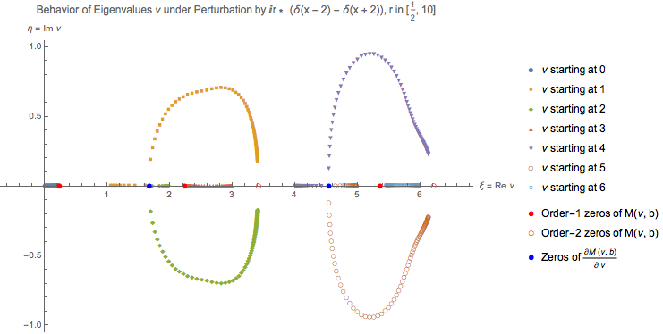
Figure 1. Some small eigenvalues of $\displaystyle L_{\text{PC}}\left(ir,2\right)$, $\displaystyle r\in\left\{\frac{1}{2}+\frac{j}{10}:0\leq j\leq 95\right\}$. Zeroes of $\displaystyle M(\nu;2)$ and its first $\displaystyle\nu$-derivative are marked. Each zero of $\displaystyle\mathsf{D}(\nu)$ eventually has a small neighborhood containing as many eigenvalues as the order of the zero.

For an entire function $\displaystyle f(\nu)$, define the maximum function $\displaystyle M_{f}(r)$, $\displaystyle r>0$, by

(5.1) $$M_{f}(r)\equiv\sup_{\left|\nu\right|=r}\left|f(\nu)\right|;$$

by the Maximum Modulus Principle, $\displaystyle M_{f}(r)=\sup_{\left|\nu\right|\leq r}\left|f(\nu)\right|$.

Remark 5.3.

It makes little difference to our entire-functions arguments whether the suppressed argument $\displaystyle b$ is real or complex; therefore, for this section only, we will let $\displaystyle\beta$ be an arbitrary complex number and redefine $\displaystyle\mathsf{D}(\nu)=D_{\nu}(\beta)$; in this more general setting, the function is still at most order-$\displaystyle 1$, maximal-type in $\displaystyle\nu$.

For the moment, we assuming the following fact about the growth rate $\displaystyle\mathsf{D}(\nu)$, to be proven later.

Lemma 5.4.

$\displaystyle\mathsf{D}(\nu)$ is of exponential order at most $\displaystyle 1$ in $\displaystyle\nu$, though possibly of maximal type; more specifically, we have the estimate,

(5.2) $$\log\left\{M_{\mathsf{D}}(r)\right\}\leq\frac{1}{4}r\log r+r\left(2+\frac{\pi}{4}\right)+O(\log r).$$

We also require the fact that $\displaystyle\mathsf{D}(\nu)$ decays as $\displaystyle\nu\to-\infty$.

Fact 5.5 (e.g., [MOS66, Chapter 8, Section 8.1.6, p. 332]).

If $\displaystyle\displaystyle\left|\arg(-\nu)\right|\leq\frac{\pi}{2}$,

(5.3) $$\mathsf{D}(\nu)=\frac{1}{\sqrt{2}}\exp\left[\frac{\nu}{2}\log(-\nu)-\frac{\nu}{2}-\beta\sqrt{-\nu}\right]\left\{1+O(\left|\nu\right|^{-1/2})\right\}.$$

In particular, for $\displaystyle\nu=-\xi$, $\displaystyle\xi>0$, we have as $\displaystyle\xi\to+\infty$ that

(5.4) $$\ln\left|\mathsf{D}(-\xi)\right|=-\frac{\xi}{2}\log(\xi)+\frac{\xi}{2}-(\operatorname{Re}\beta)\sqrt{\xi}-\frac{1}{2}\log(2)+\log\left\{1+O(\xi^{-1/2})\right\}.$$

Proof of Proposition 5.1, given Lemma 5.4.

Suppose, by way of contradiction, that $\displaystyle\mathsf{D}(\nu)$ has only finitely many zeros. Since $\displaystyle\mathsf{D}(\nu)$ is an entire function by the Weierstrass Factorization Theorem (e.g., [Lev64, Chapter 1, Section 3, Theorem 3, p. 8]), we must have

(5.5) $$\mathsf{D}(\nu)=P(\nu)e^{g(\nu)},\quad P(\nu)\text{ a polynomial, },g(\nu)\text{ entire.}$$

Yet $\displaystyle\mathsf{D}(\nu)$ is a function of order at most $\displaystyle 1$ by Lemma 5.4, so $\displaystyle g(\nu)$ must be a degree-$\displaystyle 1$ polynomial; else, it would not be order $\displaystyle 1$. Therefore,

(5.6) $$\mathsf{D}(\nu)=P(\nu)e^{c\nu+d},\quad P(\nu)\text{ a polynomial, }c,d\in\mathbb{C}.$$

Let $\displaystyle M$ be the maximum modulus of the zeroes of $\displaystyle P(\nu)$, i.e., of $\displaystyle\mathsf{D}(\nu)$. Then for $\displaystyle\nu=-\xi$, $\displaystyle\xi>M$, we must have $\displaystyle\mathsf{D}(-\xi)\neq 0$ and hence

$$\ln\left|\mathsf{D}(-\xi)\right|=\ln\left|P(-\xi)\right|-\xi\operatorname{Re}(c)+\operatorname{Re}(d)=(-\operatorname{Re}(c))\xi+O_{\beta}(\ln\xi),\quad\xi\to+\infty.$$

Yet by Fact 5.5, (5.4), $\displaystyle\ln\left|\mathsf{D}(-\xi)\right|=-\frac{\xi}{2}\log(\xi)+\frac{\xi}{2}-O_{\beta}(\sqrt{\xi})$ as $\displaystyle\xi\to+\infty$. Contradiction.

Therefore, $\displaystyle\mathsf{D}(\nu)$ has infinitely many zeros. ∎

Proof of Lemma 5.4.

We have (see [Olv61, Section 3, Theorem, (3.1), p. 813–4] ) that if $\displaystyle\nu=-a-\frac{1}{2}=\mu^{2}-\frac{1}{2}$, $\displaystyle\beta=\mu t\sqrt{2}$, and with $\displaystyle\theta=\arg\mu$, $\displaystyle\left|\theta\right|\leq\frac{\pi}{2}$,

(5.7) $$\left|D_{\mu^{2}-\frac{1}{2}}(\mu t\sqrt{2})\right|\leq k\frac{\left|(2e)^{-\,\frac{1}{4}\mu^{2}}\mu^{\frac{1}{2}\mu^{2}}\exp(-\mu^{2}\xi_{\theta}(t))\right|}{1+\left|\mu\right|^{1/6}+\left|\mu\right|^{\frac{1}{2}}\left|t^{2}-1\right|^{1/4}},$$

where $\displaystyle k$ is an unspecified constant, the powers $\displaystyle(2e)^{-\,\frac{1}{4}\mu^{2}}$ and $\displaystyle\mu^{\frac{1}{2}\mu^{2}}$ have their principal values, and $\displaystyle\xi_{\theta}(t)$ is a particular branch of the multivalued function

$$\xi(t)=\int_{1}^{t}(u^{2}-1)^{1/2}\,du=\frac{1}{2}t(t^{2}-1)^{1/2}-\frac{1}{2}\ln\{t+\sqrt{t^{2}-1}\},$$

which is defined in the following way. As we are interested in the growth rate as $\displaystyle\left|\nu\right|\to\infty$, hence $\displaystyle\left|\mu\right|=\sqrt{\left|\nu+\frac{1}{2}\right|}\to\infty$, and $\displaystyle\beta$ is fixed, we will have $\displaystyle t=\frac{x}{\mu\sqrt{2}}\to 0$. For $\displaystyle\left|t\right|\leq\frac{1}{4}$, the correct branches for our purposes are ([Olv59, Section 5, (5.8 – 5.9), p. 143], [Olv61, Section 2, (2.8 – 2.10), p. 813]),

$$\begin{split}\xi_{\theta}(t)&=\pm i\eta(t),\\ \eta(t)&=\int_{t}^{1}(1-u^{2})^{1/2}\,du=\frac{1}{2}\left(\arccos(t)-t\sqrt{1-t^{2}}\right),\\ \arccos(t)&=\int_{t}^{1}\frac{du}{\sqrt{1-u^{2}}}.\end{split}$$

More specifically, the requirements are that ([Olv61, Section 2, (2.9 – 2.10), p. 813])

$$\left\{\begin{aligned} \xi_{\theta}(0)&=-\,\frac{i\pi}{4},&&-\,\frac{\pi}{2}\leq\theta<0,\\ \xi_{0}(0+0i)&=-\,\frac{i\pi}{4},\\ \xi_{0}(0-0i)&=\frac{i\pi}{4},\\ \xi_{\theta}(0)&=\frac{i\pi}{4},\quad&&0<\theta\leq\frac{\pi}{2}.\end{aligned}\right.$$

Since $\displaystyle\eta(0)=\frac{\pi}{4}$, it follows that for $\displaystyle\theta=0$, $\displaystyle\xi_{0}(t)=i\eta(t)$ for $\displaystyle\operatorname{Im}t<0$ and $\displaystyle t$ small, and $\displaystyle\xi_{0}(t)=-i\eta(t)$ for $\displaystyle\operatorname{Im}t>0$ and $\displaystyle t$ small. As $\displaystyle\theta$ changes, the branch cut moves, but wherever it is, below the branch cut, we use $\displaystyle\xi_{\theta}(t)=i\eta(t)$, and above it we use $\displaystyle\xi_{\theta}(t)=-i\eta(t)$, and on it, we will use whichever branch gives the larger upper bound for $\displaystyle\left|\exp(-\mu^{2}\xi_{\theta}(t))\right|$.

To ensure that $\displaystyle\left|t\right|\leq\frac{1}{4}$ above, it suffices to have $\displaystyle\left|\nu\right|\geq 8\left|\beta\right|^{2}+\frac{1}{2}$, since $\displaystyle\mu^{2}=\nu+\frac{1}{2}$, or $\displaystyle\left|\mu^{2}\right|\geq\left|\nu\right|-\frac{1}{2}\geq 8\left|\beta\right|^{2}$, or $\displaystyle\left|\mu\right|\geq 2\sqrt{2}\left|\beta\right|$, and then

$$\left|t\right|=\frac{\left|\beta\right|}{\mu\sqrt{2}}\leq\frac{\left|\beta\right|}{4\left|\beta\right|}\leq\frac{1}{4}.$$

With $\displaystyle\left|t\right|\leq\frac{1}{4}$, we have that $\displaystyle\frac{\sqrt{15}}{4}\leq\left|\sqrt{1-t^{2}}\right|\leq 1$ and

$$\begin{split}\left|\arccos t\right|&\leq\left|\arccos(t)-\arccos(0)\right|+\left|\arccos(0)\right|\\ &=\left|\int_{t}^{0}\frac{du}{\sqrt{1-u^{2}}}\right|+\frac{\pi}{2}\\ &\leq\frac{\pi}{2}+\left|t\right|\cdot\frac{4}{\sqrt{15}}\leq\frac{\pi}{2}+\frac{1}{\sqrt{15}}.\end{split}$$

so that (recalling that $\displaystyle\mu^{2}=\nu+\frac{1}{2}$)

$$\begin{split}\left|-\mu^{2}\xi_{\theta}(t)\right|&\leq\left|\mu^{2}\right|\left|\pm i\right|\left|\eta(t)\right|\\ &\leq\left|\nu+\frac{1}{2}\right|\left|\frac{1}{2}\right|\left(\left|\arccos t\right|+\left|t\right|\left|\sqrt{1-t^{2}}\right|\right)\\ &\leq\left|\nu+\frac{1}{2}\right|\cdot\frac{1}{2}\cdot\left(\frac{\pi}{2}+\frac{1}{\sqrt{15}}+\frac{1}{4}\right)\\ &\leq\left|\nu+\frac{1}{2}\right|\cdot\frac{3}{2}.\end{split}$$

Thus,

(5.8) $$\left|\exp(-\mu^{2}\xi_{\theta}(t))\right|\leq\exp\left|-\mu^{2}\xi_{\theta}(t)\right|\leq\exp\left(\frac{3}{2}\left|\nu\right|+\frac{3}{4}\right).$$

To bound the other terms in the numerator of (5.7), we have

(5.9) $$\left|(2e)^{-\frac{1}{4}\mu^{2}}\right|\leq(e)^{2\cdot\left|-\frac{1}{4}\right|\cdot\left|\nu+\frac{1}{2}\right|}\leq\exp\left(\frac{1}{2}\left|\nu\right|+\frac{1}{4}\right).$$

and

(5.10) $$\begin{split}\left|\mu^{\frac{1}{2}\mu^{2}}\right|&=\left|\exp\left\{\frac{1}{2}\mu^{2}\log\mu\right\}\right|\\ &=\exp\left\{\frac{1}{2}\left|\nu+\frac{1}{2}\right|\left(\log\left|\mu\right|+\frac{\pi}{2}\right)\right\}\\ &\sim\exp\left(\frac{1}{4}\left|\nu+\frac{1}{2}\right|\log\left|\nu+\frac{1}{2}\right|+\frac{\pi}{4}\left|\nu+\frac{1}{2}\right|\right),\,\,\,\left|\nu\right|\to\infty.\end{split}$$

Therefore, combining (5.7), (5.8), (5.9), and (5.10),

$$\begin{split}\log M_{\mathsf{D}}(r)&\leq\log k+\frac{1}{2}r+\frac{1}{4}r\log r+\frac{\pi}{4}r+\frac{3}{2}r+O(\log r)\\ &=\frac{1}{4}r\log r+\left(2+\frac{\pi}{4}\right)r+O(\log r)\end{split}$$

∎

6. Eigenvalue Localization Around Non-integer Roots of $\displaystyle\mathsf{D}$

6.1. Preliminaries

We now reformulate the the first part of Lemma  3.3 as

Lemma 6.1.

If $\displaystyle\nu\not\in\mathbb{N}_{0}$ and $\displaystyle\mathsf{D}(\nu)=0$ , then $\displaystyle\Phi(\nu)\neq 0$.

As $\displaystyle\mathsf{M}(\nu)=\Gamma(-\nu)[\mathsf{D}(\nu)]^{2}\Phi(\nu)$ (see (4.21)), zeroes of $\displaystyle\mathsf{D}(\nu)$ outside $\displaystyle\mathbb{N}$ result in zeroes of exactly double the order for $\displaystyle\mathsf{M}(\nu)$, and hence should be close to solutions of $\displaystyle\mathsf{M}(\nu)=\frac{1}{z^{2}}$ for $\displaystyle\left|z\right|$ large. We compress the complex analysis into the statements below. Let $\displaystyle\lambda\in\mathbb{C}\setminus\mathbb{N}$ be a zero of order exactly $\displaystyle m$ of $\displaystyle\mathsf{D}$. Then $\displaystyle\lambda$ is a zero of order exactly $\displaystyle 2m$ of $\displaystyle\mathsf{M}$; write this function locally as

(6.1) $$\mathsf{M}(\nu)=c_{2m}(\nu-\lambda)^{2m}(1+g(\nu-\lambda)),\quad c_{2m}\neq 0,$$

where $\displaystyle g(0)=0$ and $\displaystyle g$ is analytic in some disk; fix $\displaystyle R=R(\lambda)>0$ such that $\displaystyle\left|g(\zeta)\right|\leq\frac{1}{4}$ whenever $\displaystyle\left|\zeta\right|\leq R$. Let $\displaystyle B$ be the maximum of $\displaystyle\left|g^{\prime}(\zeta)\right|$ on this neighborhood.

Lemma 6.2.

Fix $\displaystyle\rho>0$. There exists a constant $\displaystyle\delta=\delta(\lambda,\rho)$ such that if $\displaystyle\left|z\right|>\frac{1}{\delta}$, there exist $\displaystyle 2m$ solutions of $\displaystyle\mathsf{M}(\nu)=\frac{1}{z^{2}}$ (i.e., (4.20)), within the radius-$\displaystyle\rho$-neighborhood of $\displaystyle\lambda$; more precisely, if $\displaystyle\epsilon\in\mathbb{C}$ is defined such that $\displaystyle\epsilon^{2m}=\frac{1}{z^{2}c_{2m}}$, then the $\displaystyle 2m$ solutions are

(6.2) $$\nu_{j}=\lambda+\epsilon\omega^{j}+E_{j},\quad 0\leq j\leq 2m-1,\quad\omega=\exp\left(\frac{2\pi}{2m}\right),\quad\left|E_{j}\right|\leq 3B\left|\epsilon\right|^{2}.$$

In particular,

(6.3) $$\frac{1}{2}\left|\epsilon\right|\leq\left|\nu_{j}-\lambda\right|\leq 2\left|\epsilon\right|<\rho\text{ for all }j,\,\,0\leq j\leq 2m-1.$$

Proof.

Keeping in mind (6.1), and letting $\displaystyle z=\nu-\lambda$, let us analyze an equation

(.i) $$\displaystyle cz^{p}(1+g(z))=w^{p},\quad p\in\mathbb{N},c\neq 0$$

(.ii) $$\displaystyle g(0)=0,\,g\text{ analytic if }\left|z\right|\leq R,\text{ and }\left|g(z)\right|\leq\frac{1}{4}\text{ in this disc.}$$

Let

(6.5) $$B\equiv\max\{g^{\prime}(z):z\leq R\}.$$

Put

(6.6) $$h(z)=\log[1+g(z)]=\sum_{n=1}^{\infty}(-1)^{n+1}\frac{[g(z)]^{n}}{n}.$$

Then

(.i) $$\displaystyle\left|h(z)-g(z)\right|\leq\frac{2}{3}\left|g(z)\right|^{2}\leq\frac{1}{6}\left|g(z)\right|,$$

(.ii) $$\displaystyle\frac{5}{6}\left|g(z)\right|\leq\left|h(z)\right|\leq\frac{7}{6}\left|g(z)\right|<\frac{7}{6}\cdot\frac{1}{4}<\frac{1}{3},\text{ and }$$

(.iii) $$\displaystyle h^{\prime}(z)=\frac{g^{\prime}(z)}{1+g(z)},\textnormal{ so }\left|h^{\prime}(z)\right|\leq\frac{4}{3}\left|g^{\prime}(z)\right|\leq\frac{4}{3}B\text{ and }\left|h(z)\right|\leq\frac{4}{3}B\left|z\right|.$$

If $\displaystyle\omega^{p}=1$, $\displaystyle\omega=\exp\left(\frac{2\pi i}{p}\right)$, the equation (.i) splits into a series of $\displaystyle p$ equations

(6.8) $$c^{1/p}z\exp\left(\frac{1}{p}h(z)\right)=w\omega^{j},\quad 0\leq j<p,$$

where $\displaystyle c^{1/p}$ is any $\displaystyle p$th root of $\displaystyle c$. Each of them, for small enough $\displaystyle w$, has one and only one solution $\displaystyle z_{j}$, as it follows from analysis of the inverse function $\displaystyle z(\zeta)$ for

(6.9) $$z\mapsto\zeta=\mathsf{X}(z)\equiv\zeta\exp\left(\frac{1}{p}h(z)\right),\quad\left|z\right|\leq\frac{1}{4}\cdot\frac{1}{1+B};$$

it is well-defined for small $\displaystyle z$ because

$$\mathsf{X}(0)=0,\text{ and }\left.\frac{d{\mathsf{X}(z)}}{{dz}}\right|_{z=0}=1.$$

But we need good inequalities. By (6.9)

(6.10) $$z=\Psi(z;\zeta)\equiv\zeta e^{-\frac{1}{p}h(z)}=\zeta+\zeta\left[e^{-\frac{1}{p}h(z)}-1\right],$$

i.e.,

(6.11) $$z=z(\zeta)\text{ is a fixed point of }\Psi(\cdot;\zeta).$$

Claim 6.3.

If

(6.12) $$\left|\zeta\right|\leq\frac{1}{6}\cdot\frac{1}{1+B},$$

then

(6.13) $$\Psi:\mathbb{D}_{\kappa}\to\mathbb{D}_{\kappa}\text{ is contractive, for }\kappa=\frac{1}{4}\cdot\frac{1}{1+B}.$$

Proof.

Indeed, $\displaystyle e^{1/3}<\frac{3}{2}$, so

(6.14) $$\begin{split}\left|\Psi(z)\right|=\left|\zeta e^{-\,\frac{1}{p}h(z)}\right|\leq\left|\zeta\right|e^{\frac{1}{3}}<\frac{1}{6}\cdot\frac{1}{1+B}\cdot\frac{3}{2}=\frac{1}{4}\cdot\frac{1}{1+B},\end{split}$$

and for $\displaystyle z,t\in\mathbb{D}_{\kappa}$, by (.iii), (6.12)

(6.15) $$\begin{split}\left|\Psi(z)-\Psi(t)\right|&\leq\left|\zeta\right|\cdot\left|e^{-\frac{1}{p}h(z)}-e^{-\,\frac{1}{p}h(t)}\right|\\ &\leq\frac{1}{6}\cdot\frac{1}{1+B}\cdot e^{1/3}\left|h(z)-h(t)\right|\\ &\leq\frac{1}{4}\cdot\frac{1}{1+B}\cdot\frac{4}{3}\cdot B\cdot\left|z-t\right|<\frac{1}{3}\left|z-t\right|.\end{split}$$

∎

The Claim is proven. It implies the existence of $\displaystyle z(\zeta)\in\eqref{eq:fixpoint}$ which gives solutions of (6.8)

(6.16) $$z_{j}=z(\zeta_{j})=\epsilon\omega^{j},\quad\epsilon=wc^{-1/p},\quad 0\leq j<p.$$

Additional properties of $\displaystyle z(\zeta)$ come from (6.10) — and (6.14), (.ii)

(6.17) $$\begin{split}\left|z-\zeta\right|&\left|\zeta\left[e^{-\,\frac{1}{p}h(z)}-1\right]\right|\\ &\leq\left|\zeta\right|e^{1/3}\left|h(z)\right|\leq\left|\zeta\right|\cdot\frac{3}{2}\cdot B\cdot\frac{4}{3}\cdot\left|z\right|\\ &\leq\left|z\right|2B\cdot\frac{3}{2}\left|\zeta\right|\leq 3B\left|\zeta\right|^{2}.\end{split}$$

For solutions (6.16), we have if

(6.18) $$\left|\epsilon\right|\leq\frac{1}{6\left|c\right|^{1/p}}\cdot\frac{1}{1+B},$$

(6.19) $$z_{j}=\epsilon\omega^{j}+E_{j},\quad\left|E_{j}\right|\leq 3B\left|\epsilon\right|^{2},\quad 0\leq j<p.$$

So far, (6.3) has not been explained, but if $\displaystyle\left|\epsilon\right|\leq\min\{\frac{1}{6B},\frac{\rho}{3}\}$, then $\displaystyle\left|E_{j}\right|\leq 3B\left(\frac{1}{6B}\right)\left|\epsilon\right|=\frac{\left|\epsilon\right|}{2}$, and hence

$$\left|z_{j}\right|\geq\left|\epsilon\omega^{j}\right|-\left|E_{j}\right|\geq\left|\epsilon\right|\left(1-\frac{1}{2}\right)$$

and

$$\left|z_{j}\right|\leq\left|\epsilon\omega^{j}\right|+\left|E_{j}\right|\leq\left|\epsilon\right|\left(1+\frac{1}{2}\right)\leq\frac{\rho}{3}\cdot\frac{3}{2}=\frac{\rho}{2}<\rho.$$

This explains that we may take $\displaystyle\delta=\sqrt{\left|c\right|\cdot\min\{\frac{1}{(6B)^{p}},\frac{1}{\left|c\right|[6(1+B)]^{p}},\left(\frac{\rho}{2}\right)^{p}\}}$. ∎

6.2. Case: real perturbation

Suppose $\displaystyle z=r$ is real in (1.8), i.e.,

$$L_{\text{PC}}\left(r,b\right)(y(x))=-y^{\prime\prime}+\left(\frac{x^{2}}{4}-\frac{1}{2}\right)y(x)+r(\delta\left(x-b\right)-\delta\left(x+b\right)),\,\,b>0.$$

Lemma 6.4.

For $\displaystyle r\in\mathbb{R}$, $\displaystyle L_{\text{PC}}\left(r,b\right)$ is self-adjoint; consequently, $\displaystyle\operatorname{Sp}{L_{\text{PC}}\left(r,b\right)}\subseteq\mathbb{R}$.

Proof.

For real $\displaystyle r$, we now show that the quadratic form from which $\displaystyle L_{\text{PC}}\left(r,b\right)$ is formed, i.e.,

(6.20) $$\begin{split}\mathfrak{t}_{r,b}\left(u,v\right)&\equiv\left(u^{\prime}(x),v^{\prime}(x)\right)_{L^{2}(\mathbb{R})}+\frac{1}{4}\left(xu(x),xv(x)\right)_{L^{2}(\mathbb{R})}-\frac{1}{2}\left(u(x),v(x)\right)_{L^{2}(\mathbb{R})}\\ &\quad+ru(b)\overline{v(b)}-ru(-b)\overline{v(-b)}\\ \operatorname{\mathfrak{D}}\left(\mathfrak{t}_{r,b}\right)&\equiv\{f(x)\in\mathcal{H}^{1}(\mathbb{R}):xf(x)\in L^{2}(\mathbb{R})\}\end{split}$$

is semi-bounded below, i.e.,

$$\mathfrak{t}_{r,b}\left(u,u\right)\geq-c\left\|u(x)\right\|_{L^{2}(\mathbb{R})}^{2},\quad c=c(r)>0.$$

Indeed, for all $\displaystyle f\in\mathcal{H}^{1}(\mathbb{R})$, for all $\displaystyle\epsilon>0$, there exists $\displaystyle T=T(\epsilon)$ such that

(6.21) $$\sup_{x\in\mathbb{R}}\left|f(x)\right|\leq\epsilon\left\|f^{\prime}(x)\right\|_{L^{2}(\mathbb{R})}+T(\epsilon)\left\|f(x)\right\|_{L^{2}(\mathbb{R})}.$$

For $\displaystyle r=0$,

$$\begin{split}\mathfrak{t}_{0,b}\left(u,u\right)&=\left\|u^{\prime}(x)\right\|_{L^{2}(\mathbb{R})}^{2}+\frac{1}{4}\left\|xu(x)\right\|_{L^{2}(\mathbb{R})}^{2}-\frac{1}{2}\left\|u(x)\right\|_{L^{2}(\mathbb{R})}\\ &\geq-\frac{1}{2}\left\|u(x)\right\|_{L^{2}(\mathbb{R})}^{2}.\end{split}$$

For $\displaystyle r\neq 0$, we let $\displaystyle\epsilon=\frac{1}{2\sqrt{\left|r\right|}}$ and apply the inequalities (6.21) and $\displaystyle(\alpha+\beta)^{2}\leq 2(\alpha^{2}+\beta^{2})$. Then

$$\begin{split}ru(b)\overline{u(b)}=r\left|u(b)\right|^{2}&>-\left|r\right|\left(\epsilon\left\|u^{\prime}(x)\right\|_{L^{2}(\mathbb{R})}+T\left\|u(x)\right\|_{L^{2}(\mathbb{R})}\right)^{2}\\ &>-\left|r\right|\left(\frac{1}{2\sqrt{\left|r\right|}}\left\|u^{\prime}(x)\right\|_{L^{2}(\mathbb{R})}+T\left\|u(x)\right\|_{L^{2}(\mathbb{R})}\right)^{2}\\ &\geq-2\left|r\right|\left(\frac{1}{4\left|r\right|}\left\|u^{\prime}(x)\right\|_{L^{2}(\mathbb{R})}^{2}+T^{2}\left\|u(x)\right\|_{L^{2}(\mathbb{R})}^{2}\right)\\ &=-\frac{1}{2}\left\|u^{\prime}(x)\right\|_{L^{2}(\mathbb{R})}^{2}-2\left|r\right|T^{2}\left\|u(x)\right\|_{L^{2}(\mathbb{R})}^{2},\end{split}$$

and similarly for $\displaystyle-ru(-b)\overline{v(-b)}$. Therefore,

$$\begin{split}\mathfrak{t}_{r,b}\left(u,u\right)&=\left\|u^{\prime}(x)\right\|_{L^{2}(\mathbb{R})}^{2}+\frac{1}{4}\left\|xu(x)\right\|_{L^{2}(\mathbb{R})}^{2}-\frac{1}{2}\left\|u(x)\right\|_{L^{2}(\mathbb{R})}^{2}+r\left|u(b)\right|^{2}-r\left|u(-b)\right|^{2}\\ &>0-\left(4\left|r\right|T^{2}+\frac{1}{2}\right)\left\|u(x)\right\|_{L^{2}(\mathbb{R})}^{2}.\end{split}$$

Hence, in all cases, $\displaystyle\mathfrak{t}_{r,b}$ is semibounded below; as in [MS16], one checks that it is closed. Hence, the operator coming from the quadratic form is self-adjoint (e.g., [RS72, Chapter VIII, Section 6, Theorem VIII.15, p. 279]). ∎

Proposition 6.5.

1. If $\displaystyle\lambda\in\mathbb{C}$ and $\displaystyle\mathsf{D}(\lambda)=0$, then $\displaystyle\lambda>0$.

2. If $\displaystyle\lambda\in\mathbb{R}\setminus\mathbb{N}$ is a zero of $\displaystyle\mathsf{D}$, it is a simple zero.

3. If $\displaystyle\lambda\in\mathbb{R}\setminus\mathbb{N}$ is a zero of $\displaystyle\mathsf{D}$, then in the local series expansion

   $$\mathsf{M}(\nu)=c_{2}(\nu-\lambda)^{2}+O\left((\nu-\lambda)^{3}\right),$$

   $\displaystyle c_{2}>0$.

Proof, Part (i).

Fix $\displaystyle\lambda$ such that $\displaystyle\mathsf{D}(\lambda)=0$. If $\displaystyle\lambda\in\mathbb{N}$, we know that $\displaystyle\lambda$ is real, and we know that $\displaystyle\mathsf{D}(0)=D_{0}(b)=e^{-b^{2}/4}$ is nonzero, so we reduce to the case where $\displaystyle\lambda\in\mathbb{C}\setminus\mathbb{N}_{0}$. Fix $\displaystyle\rho>0$. By Lemma 6.2, for $\displaystyle r>0$ large enough such that $\displaystyle\frac{1}{r}<\delta(\lambda,\rho)$, there exist several solutions of $\displaystyle\mathsf{M}(\nu)=\frac{1}{r^{2}}$ within $\displaystyle\rho$ of $\displaystyle\lambda$. Yet these solutions cannot be nonnegative integers, for $\displaystyle\mathsf{M}(\nu)$ is not defined on the nonnegative integers. Therefore, by Corollary 4.6, these solutions are eigenvalues of $\displaystyle L_{\text{PC}}\left(r,b\right)$, and by Lemma 6.4, such eigenvalues must be real numbers. Therefore, we have that the distance from $\displaystyle\lambda$ to the real line is bounded above by the distance from $\displaystyle\lambda$ to $\displaystyle\operatorname{Sp}{L_{\text{PC}}\left(r,b\right)}$, which is at most $\displaystyle\rho$ for sufficiently large $\displaystyle r$. As $\displaystyle\rho>0$ is arbitrary, we must have $\displaystyle\lambda\in\mathbb{R}$.

Moreover, by the integral representation from (3.4) (e.g., [MOS66, Section 8.1.4, p. 328]), if $\displaystyle\nu<0$, then

$$\mathsf{D}(\nu)=\frac{e^{-b^{2}/4}}{\Gamma(-\nu)}\int_{0}^{\infty}t^{-\nu-1}e^{-t^{2}/2-bt}\,dt,$$

which is a nonzero constant times the integral of a positive integrand, and hence is nonzero. Therefore, the zeroes of $\displaystyle\mathsf{D}(\nu)$ avoid the negative real axis, and as already noted, $\displaystyle 0$ is not a zero of $\displaystyle\mathsf{D}(\nu)$, so $\displaystyle\lambda>0$. ∎

Proof, Part (ii).

Assume $\displaystyle m>1$, $\displaystyle 2m>2$. By Lemma 6.2, see (4.20), even if $\displaystyle z$ is real, with

(6.22) $$\mathsf{M}(\nu)=c_{2m}(\nu-\lambda)^{2m}(1+g(\nu-\lambda)),\quad c_{2m}\neq 0,$$

(6.23) $$\epsilon^{2m}=\frac{1}{z^{2}c_{2m}},\text{ or }\epsilon=\left(\frac{1}{z^{2}}\right)^{1/2m}c_{2m}^{-1/2m},\quad\left|z\right|\gg 1,$$

($\displaystyle c_{2m}^{-1/2m}$ is any $\displaystyle 2m$th root of $\displaystyle c_{2m}^{-1}$), we have eigenvalues

(6.24) $$\begin{split}\nu_{j}&=\lambda+\epsilon\omega^{j}+E_{j},\quad\left|E_{j}\right|\leq 3B\left|\epsilon\right|^{2},\quad 0\leq j<2m\\ &=\lambda+\epsilon\omega^{j}(1+\tau_{j}\epsilon),\quad\left|\tau_{j}\right|\leq 3B\left|\epsilon\right|,\quad 0\leq j<2m\end{split}$$

Therefore,

(6.25) $$\arg\left(\nu_{j}-\lambda\right)=\arg(\epsilon)+\frac{2\pi}{2m}j+\sigma_{j}\quad\left|\sigma_{j}\right|\leq 6B\left|\epsilon\right|,\quad 0\leq j<2m.$$

and for $\displaystyle\epsilon$, $\displaystyle\left|\epsilon\right|<\frac{1}{12B}\cdot\frac{\pi}{m}$, at most $\displaystyle 2$ numbers in $\displaystyle\{\nu_{j}\}_{j=0}^{2m-1}$, $\displaystyle\nu_{j}\in\eqref{eq:localrootexpansionredo}$, are real. With $\displaystyle 2m\geq 4>2$ we would get a non-real eigenvalue of the self-adjoint operator $\displaystyle L_{\text{PC}}\left(z,b\right)$. This contradiction implies that $\displaystyle m=1$. ∎

Proof, Part (iii).

Moreover, the same analysis shows that for $\displaystyle m=1$ the coefficient $\displaystyle c_{2}\neq 0$ should be positive: $\displaystyle c_{2}>0$. Otherwise (i.e., with $\displaystyle c_{2}<0$), by (6.23) with positive $\displaystyle z>0$, $\displaystyle z\gg 1$,

(6.26) $$\epsilon^{2}=\frac{1}{z^{2}c_{2}},\text{ and }\epsilon=\pm\frac{1}{\sqrt{c_{2}}}\cdot\frac{1}{z}\text{ is \emph{not} real.}$$

By (6.24)

(6.27a) $$\displaystyle\nu_{0} \displaystyle=\lambda+\epsilon+E_{0}=\lambda+\epsilon(1+s_{0})$$

(6.27b) $$\displaystyle\nu_{1} \displaystyle=\lambda-\epsilon+E_{1}=\lambda-\epsilon(1+s_{1}),$$

where

(6.28) $$\left|s_{j}\right|\leq\left(\frac{3B}{\left|c_{2}\right|^{1/2}}\right)\cdot\frac{1}{\left|z\right|}.$$

For $\displaystyle z>1$ large enough, both eigenvalues $\displaystyle\nu_{0}$, $\displaystyle\nu_{1}$ would not be real.

∎

6.3. Case: Pure Imaginary perturbation

We now discuss $\displaystyle L_{\text{PC}}\left(ir,b\right)$, $\displaystyle r\in\mathbb{R}$, $\displaystyle b>0$, as in (1.8).

Proposition 6.6.

Fix $\displaystyle\lambda\in\mathbb{R}_{>0}\setminus\mathbb{N}_{0}$ such that $\displaystyle\mathsf{D}(\lambda)=0$, and fix $\displaystyle\rho>0$. For $\displaystyle r>\frac{1}{\delta(\lambda,\rho)}$, there exists $\displaystyle 2$ nonreal eigenvalues of $\displaystyle L_{\text{PC}}\left(ir,b\right)$ in a radius-$\displaystyle\rho$ neighborhood of $\displaystyle\lambda$.

Proof.

We repeat the above analysis. Let $\displaystyle z=ir$; then (6.26) becomes

(6.29) $$\epsilon^{2}=\frac{1}{z^{2}c_{2}}=-\,\frac{1}{r^{2}c_{2}},\text{ and }\epsilon=\pm\frac{1}{\sqrt{c_{2}}}\cdot\frac{i}{r}\text{ is \emph{not} real, by }\sqrt{c_{2}}\text{ real.}$$

Then (6.27) and (6.28) still hold; hence, for $\displaystyle r$ large enough, the solutions of $\displaystyle\mathsf{M}(\nu)=\frac{1}{(ir)^{2}}$ near $\displaystyle\lambda$ are non-real. Yet by Corollary 4.6, these solutions are eigenvalues of $\displaystyle L_{\text{PC}}\left(ir,b\right)$. By Lemma 6.2, for $\displaystyle r$ large enough, the non-real eigenvalues are within $\displaystyle\rho$ of $\displaystyle\lambda$. ∎

7. Eigenvalue Localization around Integer Zeros of $\displaystyle\mathsf{D}$

7.1. One Guaranteed Zero, and Several Nearby Zeros

Although $\displaystyle D_{0}(x)=e^{-x^{2}/4}$ is never zero, it is certainly possible that $\displaystyle D_{n}(b)=0$ for $\displaystyle n\in\mathbb{N}$; indeed, $\displaystyle D_{2}(1)=0$.

By Corollary 4.6, (4.19), $\displaystyle\nu\in\operatorname{Sp}{L_{\text{PC}}\left(z,b\right)}$ if and only if

$$\frac{1}{\Gamma(-\nu)}-z^{2}\mathsf{D}(\nu)\Phi(\nu)=0.$$

If $\displaystyle\mathsf{D}(n)=0$, then $\displaystyle n\in\operatorname{Sp}{L_{\text{PC}}\left(z,b\right)}=0$ for all $\displaystyle z$, for the left-hand-side of the above equation becomes

$$\frac{1}{\Gamma(-n)}-z^{2}\mathsf{D}(n)\Phi(n)=0-z^{2}\cdot 0=0.$$

Lemma 7.1.

If $\displaystyle n\in\mathbb{N}$ is a zero of $\displaystyle\mathsf{D}$, then $\displaystyle n\in\operatorname{Sp}{L_{\text{PC}}\left(z,b\right)}$ for all $\displaystyle z\in\mathbb{C}$.

We claim, however, that neighborhoods of such integer zeros of $\displaystyle\mathsf{D}$ work in much the same way as non-integer zeros of $\displaystyle\mathsf{D}$ as a starting point for finding non-real eigenvalues of $\displaystyle\operatorname{Sp}{L_{\text{PC}}\left(ir,b\right)}$.

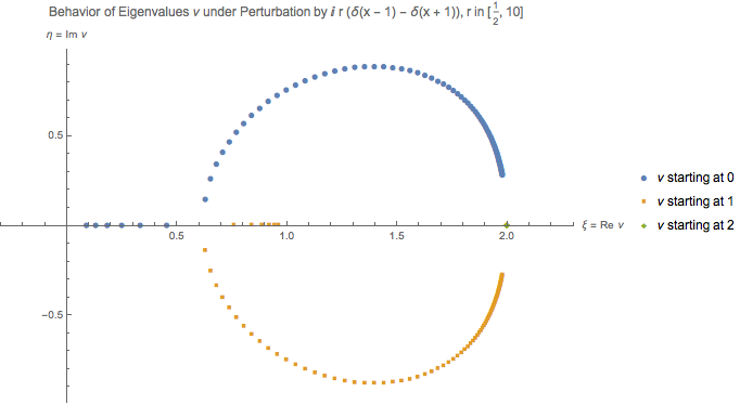
Figure 2. A graph of several eigenvalues of $\displaystyle L_{\text{PC}}\left(ir,1\right)$ for $\displaystyle r\in\left\{\frac{1}{2}+\frac{j}{10}:0\leq j\leq 95\right\}$. As $\displaystyle r$ increases, two of the eigenvalues are close to $\displaystyle n=2$, but are non-real.

Numerical evidence for this in the case $\displaystyle b=1$ is given by Figure 2.

The key observation is the second part of Lemma 3.3, revised here as

Lemma 7.2.

If $\displaystyle n\in\mathbb{N}$, and $\displaystyle\mathsf{D}(n)=0$, then $\displaystyle\Phi(n)=0$.

Thus, if $\displaystyle n\in\mathbb{N}$ is a zero of $\displaystyle\mathsf{D}$ of order $\displaystyle m\geq 1$, then $\displaystyle n$ is a zero of $\displaystyle\Phi$ of order $\displaystyle q\geq 1$. Then $\displaystyle[\mathsf{D}(\nu)]^{2}\Phi(\nu)$ has a zero of order at least $\displaystyle 2m+q\geq 3$ at $\displaystyle\nu=n$, and thus $\displaystyle\mathsf{M}(\nu)=\Gamma(-\nu)[\mathsf{D}(\nu)]^{2}\Phi(\nu)$ (see (4.21)) has a removable singularity at $\displaystyle n$ and can be analytically continued there, with a zero of order $\displaystyle 2m+q-1\geq 2$ at $\displaystyle n$. We call this extended function $\displaystyle\mathbf{M}(\nu)$ for clarity; write this function locally as

(7.1) $$\mathbf{M}(\nu)=c_{2m+q-1}(\nu-n)^{2m+q-1}(1+g(\nu-n)),\quad c_{2m+q-1}\neq 0,$$

where $\displaystyle g(0)=0$ and $\displaystyle g$ is analytic in some disk; fix $\displaystyle R>0$ such that $\displaystyle\left|g(\xi)\right|\leq\frac{1}{4}$ whenever $\displaystyle\left|\xi\right|\leq R$, and let $\displaystyle B$ the maximum of $\displaystyle g^{\prime}(\xi)$ on this interval. We now establish the analogue of Lemma 6.2 for $\displaystyle\mathbf{M}(\nu)$.

Lemma 7.3.

Fix $\displaystyle\rho$, $\displaystyle 0<\rho<\frac{1}{2}$, and suppose that $\displaystyle\mathsf{D}(n)=0$ for $\displaystyle n\in\mathbb{N}$. Then there exists a constant $\displaystyle\delta(n,\rho)$ such that if $\displaystyle\left|z\right|>\frac{1}{\delta(n)}$, there exist $\displaystyle 2m+q-1$ solutions of $\displaystyle\mathsf{M}(\nu)=\frac{1}{z^{2}}$ (i.e., (4.20)), within the radius - $\displaystyle\rho$ - neighborhood of $\displaystyle\lambda$; more precisely, if $\displaystyle\epsilon\in\mathbb{C}$ is defined such that $\displaystyle\epsilon^{2m+q-1}=\frac{1}{z^{2}c_{2m+q-1}}$, then the $\displaystyle 2m+q-1$ solutions are

(7.2) $$\begin{split}\nu_{j}&=n+\epsilon\omega^{j}+E_{j},\quad 0\leq j<2m+q-1,\\ \omega&=\exp\left(\frac{2\pi}{2m+q-1}\right),\quad\left|E_{j}\right|\leq 3B\left|\epsilon\right|^{2}.\end{split}$$

In particular,

(7.3) $$\frac{1}{2}\left|\epsilon\right|\leq\left|\nu_{j}-n\right|\leq 2\left|\epsilon\right|<\frac{1}{2}\text{ for all }j,\,\,0\leq j<2m+q-1.$$

Proof.

By repeating the proof of Lemma 6.2, for sufficiently large $\displaystyle z$, there exist $\displaystyle 2m+q-1$ solutions of $\displaystyle\mathbf{M}(\nu)=\frac{1}{z^{2}}$ with the above properties. However, by the first inequality of (7.3), none of the solutions $\displaystyle\nu_{j}$ are equal to $\displaystyle n$ and by the latter two inequalities, $\displaystyle\left|\nu_{j}-n\right|<\rho<\frac{1}{2}<1$, no solution $\displaystyle\nu_{j}$ can equal any integer other than $\displaystyle n$. Therefore, no $\displaystyle\nu_{j}$ is integer, which means that the solutions are solutions of the unextended equation $\displaystyle\mathsf{M}(\nu)=\frac{1}{z^{2}}$ as well. ∎

7.2. Case: Real Perturbation

We now prove the analogue of Proposition 6.5 for integer zeros of $\displaystyle\mathsf{D}$.

Proposition 7.4.

1. If $\displaystyle n\in\mathbb{N}$ is a zero of $\displaystyle\mathsf{D}$ of order $\displaystyle m$, and it is a zero of $\displaystyle\Phi$ of order $\displaystyle q$, then both zeros are simple; i.e., $\displaystyle\mathbf{M}$ has a zero of order exactly $\displaystyle 2$ there.

2. If $\displaystyle n\in\mathbb{N}$ is a zero of $\displaystyle\mathsf{D}$, then in the series expansion

   $$\mathbf{M}(\nu)=c_{2}(\nu-n)^{2}+O\left((\nu-n)^{3}\right),$$

   $\displaystyle c_{2}>0$.

Proof, part (i).

If $\displaystyle n\in\mathbb{N}$ is a zero of $\displaystyle\mathsf{D}$ of order $\displaystyle m$, and $\displaystyle n$ is a zero of $\displaystyle\Phi$ of order $\displaystyle q$, then the order of the zero of $\displaystyle\mathbf{M}$ at $\displaystyle n$ is $\displaystyle 2m+q-1$, since $\displaystyle[\mathsf{D}(\nu)]^{2}$ gives a zero of order $\displaystyle 2m$ at $\displaystyle n$, and $\displaystyle\Gamma(-\nu)$ takes away an order of the zero. Thus, let us write $\displaystyle\mathbf{M}$ locally as

(7.4) $$\mathbf{M}(\nu)=c_{2m+q-1}(\nu-n)^{2m+q-1}(1+g(\nu-\lambda)),\quad c_{2m+q-1}\neq 0.$$

Let

(7.5) $$\epsilon^{2m+q-1}=\frac{1}{z^{2}c_{2m+q-1}},\text{ or }\epsilon=\left(\frac{1}{z^{2}}\right)^{1/(2m+q-1)}c_{2m+q-1}^{-1/(2m+q-1)},\left|z\right|\gg 1,$$

where $\displaystyle c_{2m+q-1}^{-1/(2m+q-1)}$ is any $\displaystyle 2m+q-1$th root of $\displaystyle c_{2m+q-1}^{-1}$. By Lemma 7.3, letting $\displaystyle z$ be real, there exist $\displaystyle 2m+q-1$ solutions of $\displaystyle\mathbf{M}(\nu)=\frac{1}{z^{2}}$ in a radius-$\displaystyle\frac{1}{2}$-neighborhood of $\displaystyle n$, namely

(7.6) $$\begin{split}\nu_{j}&=n+\epsilon\omega^{j}+E_{j},\left|E_{j}\right|\leq 3B\left|\epsilon\right|^{2},\quad 0\leq j<2m+q-1,\\ &=n+\epsilon\omega^{j}(1+\tau_{j}\epsilon),\quad\left|\tau_{j}\right|\leq 3B\left|\epsilon\right|,0\leq j<2m+q-1,\end{split}$$

where $\displaystyle\omega=\exp\left(\frac{2\pi}{2m+q-1}\right)$. By Corollary 4.6, these solutions are eigenvalues of $\displaystyle L_{\text{PC}}\left(z,b\right)$, and by Lemma 6.4, they are real.

Therefore,

(7.7) $$\arg(\nu_{j}-n)=\frac{2\pi}{2m+q-1}j+\sigma_{j},\,\l,\left|\sigma_{j}\right|\leq 6B\left|\epsilon\right|,\,\,0\leq j<2m+q-1,$$

and for $\displaystyle\epsilon$ such that $\displaystyle\left|\epsilon\right|<\frac{1}{12B}\cdot\frac{2\pi}{2m+q-1}$, at most $\displaystyle 2$ numbers in $\displaystyle\{\nu_{j}\}_{j=0}^{2m+q-2}$, $\displaystyle\nu_{j}\in\eqref{eq:localsolInt}$, are real. With $\displaystyle 2m+q-1\geq 3>2$, we would get a non-real eigenvalue of the self-adjoint operator $\displaystyle L_{\text{PC}}\left(z,b\right)$. This contradiction implies that $\displaystyle 2m+q-1\leq 2$, and with $\displaystyle m\geq 1$, $\displaystyle q\geq 1$, the only resolution is $\displaystyle m=q=1$; i.e., both roots are simple. ∎

Proof, part (ii).

For $\displaystyle m=q=1$, the coefficient $\displaystyle c_{2}\neq 0$ should be positive: i.e., $\displaystyle c_{2}>0$. Otherwise, by (7.5), with positive $\displaystyle z$, $\displaystyle z\gg 1$,

(7.8) $$\epsilon^{2}=\frac{1}{z^{2}c_{2}},\,\text{ and }\epsilon=\pm\frac{1}{\sqrt{c_{2}}}\cdot\frac{1}{z}\text{ is \emph{not} real.}$$

By (7.6),

(7.9) $$\begin{split}\nu_{0}&=n+\epsilon+E_{0}=\lambda+\epsilon(1+s_{0})\\ \nu_{1}&=n-\epsilon+E_{1}=\lambda-\epsilon(1+s_{1})\\ \end{split}$$

where

(7.10) $$\left|s_{j}\right|\leq\left(\frac{3B}{\left|c_{2}\right|^{1/2}}\right)\cdot\frac{1}{\left|z\right|}.$$

For $\displaystyle z>1$ large enough, both solutions $\displaystyle\nu_{0}$, $\displaystyle\nu_{1}$ would not be real, but they are real, again by Corollary 4.6 and Lemma 6.4. ∎

7.3. Case: Imaginary Perturbation

Proposition 7.5.

If $\displaystyle n\in\mathbb{N}$ is such that $\displaystyle\mathsf{D}(n)=0$, and $\displaystyle\rho>0$, then for $\displaystyle r>\frac{1}{\delta(n,\rho)}$, there exists $\displaystyle 2$ nonreal eigenvalues of $\displaystyle L_{\text{PC}}\left(ir,b\right)$ (see (1.8)) in the radius-$\displaystyle\rho$-neighborhood of $\displaystyle n$.

Proof.

We repeat the above analysis. If $\displaystyle z=ir$, then (7.8) becomes

$$\epsilon^{2}=\frac{1}{z^{2}c_{2}}=-\,\frac{1}{r^{2}c_{2}},\text{ and }\epsilon=\pm\frac{1}{\sqrt{c_{2}}}\cdot\frac{i}{r}\text{ is \emph{not} real, by }\sqrt{c_{2}}\text{ real.}$$

Then (7.9) and (7.10) still hold; hence, for $\displaystyle r$ large enough, the solutions of $\displaystyle\mathsf{M}(\nu)=\frac{1}{(ir)^{2}}$ near $\displaystyle n$ are non-real. yet by Corollary 4.6, these solutions are eigenvalues of $\displaystyle L_{\text{PC}}\left(ir,b\right)$. ∎

8. Proof of Theorem 1

Consider the family of operators $\displaystyle L_{\text{PC}}\left(re^{i\pi/2},b\right)=L_{\text{PC}}\left(ir,b\right)$. Consider the first $\displaystyle p$ roots $\displaystyle 0<\lambda_{1}<\dotsc<\lambda_{p}$ of $\displaystyle\mathsf{D}(\nu)$. By Lemma 6.2 and Proposition 6.5 (or Lemma 7.3 and Proposition 7.4), for each $\displaystyle q$, $\displaystyle 1\leq q\leq p$, the equation $\displaystyle\mathsf{M}(\nu)=\frac{1}{z^{2}}$ (or $\displaystyle\mathbf{M}(\nu)=\frac{1}{z^{2}}$) is of the form

(8.1) $$c_{2}(\nu-\lambda_{q})^{2}[1+g_{q}(\nu-\lambda_{q})]=\frac{1}{(ir)^{2}}=-\frac{1}{r^{2}},\quad c_{2}>0,$$

where $\displaystyle g(z)\leq C_{3}$ if $\displaystyle\left|z\right|\leq\rho_{q}$, and we may enforce $\displaystyle\rho_{q}<\frac{1}{2}\min_{2\leq q\leq p}\lambda_{q}-\lambda_{q-1}$. By Propositions 6.6 and 7.5, for each $\displaystyle q$, $\displaystyle 1\leq q\leq p$, there exists a constant $\displaystyle\delta(\lambda_{q},\rho_{q})$ such that for $\displaystyle r>\frac{1}{\delta(\lambda_{q},\rho_{q})}$, there exist $\displaystyle 2$ non-real solutions of (8.1) in the radius-$\displaystyle\rho_{q}$-neighborhood of $\displaystyle\lambda_{q}$ (call them $\displaystyle\kappa_{j}^{(q)}(r)$), $\displaystyle j=0,1$), and by Corollary 4.6, these solutions are eigenvalues of $\displaystyle\operatorname{Sp}{L_{\text{PC}}\left(ir,b\right)}$. Moreover, by $\displaystyle\rho_{q}<\frac{1}{2}\min_{2\leq q\leq p}\lambda_{q}-\lambda_{q-1}$, these neighborhoods are disjoint, so if $\displaystyle q\neq t$, $\displaystyle\kappa_{j}^{(q)}(r)\neq\kappa_{k}^{(t)}(r)$, $\displaystyle j,k$ in $\displaystyle\{0,1\}$. Therefore, we see that for some $\displaystyle r^{*}$,

(8.2) $$r\geq r^{*}\Rightarrow\#\left(\operatorname{Sp}L_{\text{PC}}\left(ir,b\right)\setminus\mathbb{R}\right)\geq 2p.$$

This holds for all $\displaystyle p\in\mathbb{N}$, so letting

$$\mathcal{N}_{\textnormal{PC}}(r)=\mathcal{N}_{\textnormal{PC}}(r;b)\equiv\#\left(\operatorname{Sp}L_{\text{PC}}\left(ir,b\right)\setminus\mathbb{R}\right),$$

we have the following.

Theorem 8.1.

$\displaystyle\lim_{r\to\infty}\mathcal{N}_{\textnormal{PC}}(r;b)=\infty$.

By the change of variables in Section 1.2, we establish Theorem 1, as well; i.e., $\displaystyle\lim_{r\to\infty}\mathcal{N}_{\textnormal{HO}}(r)=\infty$.

9. Conclusion

Two general questions should be clarified.

First, we know that

(9.1) $$\displaystyle\mathcal{N}(r) \displaystyle\leq c(r\log(er))^{2}$$ [Mit15, Thm. 4.4, (4.38), p. 4082],

and

(9.2) $$\displaystyle\lim_{r\to\infty}\mathcal{N}(r) \displaystyle=\infty$$ Theorem 1, (1.5), p. 1 above.

But the gap between the estimates for $\displaystyle\mathcal{N}$ from above and below is too wide.

Second, how to the eigenvalues $\displaystyle\lambda(ir)$ move, $\displaystyle 0\leq r<\infty$? Sections 6, 7 tell a lot about $\displaystyle\lambda(ir)$, $\displaystyle r\gg 1$, close to zeros of $\displaystyle\mathsf{D}$. But, for example, could some $\displaystyle\lambda_{j}(ir)$, $\displaystyle 0\leq r\ll 1$, go to $\displaystyle\infty$ when $\displaystyle r\to\infty$? Numerics hint that it could not happen, but there is no formal (rigorous) argument to explain this phenomenon.

Ran

pages43 Ranpages-1 Ranpages10 Ranpages4 Ranpages6 Ranpages-1 Ranpages-1 Ranpages18 Ranpages45 Ranpages-1 Ranpages21 Ranpages39 Ranpages12 Ranpages-1 Ranpages-1

References

- [BM18] Charles E. Baker and Boris S. Mityagin “Localization of eigenvalues of doubly cyclic matrices” In Linear Algebra and its Applications 540, 2018, pp. 160–202 DOI: https://doi.org/10.1016/j.laa.2017.11.016
- [Con78] John B. Conway “Functions of one complex variable” 11, Graduate Texts in Mathematics Springer-Verlag, New York-Berlin, 1978, pp. xiii+317
- [Dea66] P. Dean “The constrained quantum mechanical harmonic oscillator” In Mathematical Proceedings of the Cambridge Philosophical Society 62, 1966, pp. 277–286 DOI: 10.1017/S0305004100039840
- [Dem05] Ersan Demiralp “Properties of a pseudo-Hermitian Hamiltonian for harmonic oscillator decorated with Dirac delta interactions” In Czechoslovak J. Phys. 55.9, 2005, pp. 1081–1084 DOI: 10.1007/s10582-005-0110-2
- [HCW14] Daniel Haag, Holger Cartarius and Günter Wunner “A Bose-Einstein Condensate with -Symmetric Double-Delta Function Loss and Gain in a Harmonic Trap: A Test of Rigorous Estimates” In Acta Polytechnica 54.2 Czech Technical University in Prague, 2014, pp. 116–121 DOI: doi:10.14311/AP.2014.54.0116
- [Kat95] Tosio Kato “Perturbation theory for linear operators” Reprint of the 1980 edition, Classics in Mathematics Springer-Verlag, Berlin, 1995, pp. xxii+619
- [Lev64] B.. Levin “Distribution of zeros of entire functions” 5, Translations of Mathematical Monographs American Mathematical Society, Providence, R.I., 1964, pp. viii+493
- [Mit15] Boris Mityagin “The Spectrum of a Harmonic Oscillator Operator Perturbed by Point Interactions” In International Journal of Theoretical Physics 54, 2015, pp. 4068–4085 URL: http://link.springer.com/article/10.1007/s10773-014-2468-z
- [Mit16] Boris S. Mityagin “The spectrum of a harmonic oscillator operator perturbed by -interactions” In Integral Equations Operator Theory 85.4, 2016, pp. 451–495 DOI: 10.1007/s00020-016-2307-0
- [MOS66] Wilhelm Magnus, Fritz Oberhettinger and Raj Pal Soni “Formulas and theorems for the special functions of mathematical physics”, Third enlarged edition. Die Grundlehren der mathematischen Wissenschaften, Band 52 Springer-Verlag New York, Inc., New York, 1966, pp. viii+508
- [MS16] Boris Mityagin and Petr Siegl “Root system of singular perturbations of the harmonic oscillator type operators” In Lett. Math. Phys. 106.2, 2016, pp. 147–167 DOI: 10.1007/s11005-015-0805-7
- [Olv59] F… Olver “Uniform asymptotic expansions for Weber parabolic cylinder functions of large orders” In J. Res. Nat. Bur. Standards Sect. B 63B, 1959, pp. 131–169
- [Olv61] F… Olver “Two inequalities for parabolic cylinder functions” In Proc. Cambridge Philos. Soc. 57, 1961, pp. 811–822
- [Olv74] F… Olver “Asymptotics and special functions” Computer Science and Applied Mathematics Academic Press [A subsidiary of Harcourt Brace Jovanovich, Publishers], New York-London, 1974, pp. xvi+572
- [RS72] Michael Reed and Barry Simon “Methods of modern mathematical physics. I. Functional analysis” Academic Press, New York-London, 1972, pp. xvii+325
- [Tem19] N.. Temme “Chapter 12 Parabolic Cylinder Functions”, 2019 URL: http://dlmf.nist.gov/12