11institutetext: Facultad de Ciencias Exactas, Ingeniería y Agrimensura, Universidad Nacional de Rosario, Av. Pellegrini 250, Rosario, Argentina. 22institutetext: Instituto de Astronomía y Física del Espacio (IAFE). CONICET-Universidad de Buenos Aires. Buenos Aires, Argentina. 33institutetext: Instituto de Física de Rosario (IFIR). CONICET-Universidad Nacional de Rosario. Rosario, Argentina. 44institutetext: Facultad de Ciencias Astronómicas y Geofísicas, Universidad Nacional de La Plata. Paseo del Bosque s/n. La Plata. Argentina.

The dynamical evolution of close-in binary systems formed by a super-Earth and its host star

Case of the Kepler-21 system
S. H. Luna Corresponding author (Santiago Luna): santiagohluna@gmail.com1122    H. D. Navone 1133    M. D. Melita 2244
(Received …; accepted …)
Abstract

Aims. The aim of this work is to develop a formalism for the study of the secular evolution of a binary system which includes interaction due to the tides that each body imparts on the other. We also consider the influence of the J2subscript𝐽2J_{2}-related secular terms on the orbital evolution and the torque, caused by the triaxiality, on the rotational evolution, both of which are associated only to one of the bodies. We apply these set of equations to the study of the orbital and rotational evolution of a binary system composed of a rocky planet and its host star in order to characterize the dynamical evolution at work, particularly near spin-orbit resonances.

Methods. We used the equations of motion that give the time evolution of the orbital elements and the spin rates of each body to study the time evolution of the Kepler-21 system as an example of how the formalism that we have developed can be applied.

Results. We obtained a set of equations of motion without singularities for vanishing eccentricities and inclinations. This set gives, on one hand, the time evolution of the orbital elements due to the tidal potentials generated by both members of the system as well as the triaxiality of one of them. On the other hand, it gives the time evolution of the stellar spin rate due to the corresponding tidal torque and of the planet’s rotation angle due to both the tidal and triaxiality-induced torques. We found that for the parameters and the initial conditions explored here, the tidally and triaxiality-induced modifications of the tidal modes can be more significative than expected and that the time of tidal synchronization strongly depends on the values of the rheological parameters.

Key Words.:
Celestial mechanics – Planet-Star interactions – Planets and satellites: dynamical evolution and stability – Planets and satellites: terrestrial planets – Planets and satellites: individual: Kepler-21b

1 Introduction

Recent developments and improvements in the field of exoplanet detection methods have allowed for the discovery of many Earth-sized planets, so-called super-Earths, which have masses between 111 and 10M10subscript𝑀direct-sum10\,M_{\oplus}. This has given rise to an interest in other, related topics, such as the dynamical and thermal evolution (Stamenković et al., 2012; Shoji & Kurita, 2014; Makarov et al., 2018; Renaud & Henning, 2018), the presence of atmospheres (Seager, 2010), the internal structure and composition (Valencia et al., 2006, 2007b, 2007a), and the possibility that these types of celestial bodies offer for harboring life.

In this work, we are interested in the first of these problems, that is, the dynamical evolution of a binary system formed by a super-Earth and its host star, modeled as bodies that are capable of experiencing internal stresses and energy dissipation. Our aim is to develop a set of equations of motion to study the orbital and rotational evolution of such a system due to the tides that each celestial body induces on the other and the triaxiality of the planet itself. We are particularly interested in the dynamical evolution near spin orbit-resonances. For this reason, we have derived the equations of motion that give, on one hand, the time evolution of the orbital elements due to the secular terms of both the tidal and the J2subscript𝐽2J_{2}-related disturbing potentials and, on the other hand, the time evolution of the stellar rotation rate and that of the rotation angle of the planet, which are both due to the secular terms of the corresponding tidal torque and to the triaxiality-induced torque on the latter.

Certainly, we expect that close-in planets ends their rotational history in the 1:1 spin-orbit resonance, that is, when θ˙=n,˙𝜃𝑛\dot{\theta}=n, where θ˙˙𝜃\dot{\theta} is the spin rate of the considered body and n𝑛n is the the mean orbital frequency, which, in the unperturbed two point-masses problem, is defined by the mathematical expression of the Kepler’s third law:

G(m1+m2)=n2a3,𝐺subscript𝑚1subscript𝑚2superscript𝑛2superscript𝑎3G\left(m_{1}+m_{2}\right)=n^{2}a^{3}, (1)

where G𝐺G is the universal gravitation constant. Yet, as we shall see later, a rotating body may get trapped in higher-than-synchronous rotation states (Efroimsky, 2012) and that the eccentricity plays a key role in the possibility of capture in spin-orbit resonances, as shown by Goldreich & Peale (1966); Efroimsky (2012); Makarov (2012); Makarov et al. (2012); Noyelles et al. (2014).

Resonant capture in spin-orbit resonances is a phenomenon that occurs due to the interplay between the tidal and the triaxiality-induced torques. The former torque is due to the tides that each component of the binary system induces on the other, while the latter is characterized by the principal moments of inertia of at least one of them. Naturally, here, we consider super-Earths as triaxial bodies because they probably have a rocky composition, in contraposition to the stars, which are expected to be fluid.

This work is organized as follows: In Sect. 2, we present the equations of motion in its general form as were derived by Boué & Efroimsky (2019). We also explicitly give the tidal and triaxial potentials and the rheological models for each component. In Sect. 3, we derive the equations that have to be solved numerically in order to obtain the time evolution of the particular system under study, which have the particularity of being regular for very small and null eccentricities and inclinations. In Sect. 4, we discuss the choice of the values of the physical and rheological parameters involved and the initial conditions for the numerical integration. In Sect. 5, we study the dynamical evolution of the Kepler-21 system as an example of application of the developed methodology. Also, we present and discuss the results obtained from the numerical integration of the equations of motion mentioned above and evaluate the possibility of detecting tidal effects. Finally, in Sect. 6, we offer a final discussion and draw our conclusions.

2 Generalities

To describe the dynamical evolution, including the orbital and rotational motions, of a binary system constituted of a rocky planet and its host star, we make use of the equations of motion derived by Boué & Efroimsky (2019), which are valid for the case when the tidal dissipation within both bodies is considered, including the disturbing potential due to the permanent-triaxial shape of the planet.

We consider a system of two bodies, the host star and a rocky planet. Each body is thought of as a nearly spherical mass distribution characterized by its principal moments of inertia, total mass, and mean radius. The former is assumed to have total mass, m1subscript𝑚1m_{1}, and radius, R1subscript𝑅1R_{1}, and the latter has the total mass, m2subscript𝑚2m_{2}, and radius, R2subscript𝑅2R_{2}. The corresponding principal moments of inertia of each body is represented by Aksubscript𝐴𝑘A_{k}, Bksubscript𝐵𝑘B_{k}, and Cksubscript𝐶𝑘C_{k} (with k=1,2𝑘12k=1,2 and A<B<C𝐴𝐵𝐶A<B<C). The index, k𝑘k, identifies each body: k=1𝑘1k=1 corresponds to the star-related parameters and variables, while k=2𝑘2k=2 corresponds to the planet-related ones.

The mutual orbit is parameterized by the six classical orbital elements: the major semiaxis (a𝑎a), the eccentricity (e𝑒e), the mean anomaly (M𝑀M), the argument of pericenter (ω𝜔\omega), the inclination (i𝑖i), and the longitude of the ascending node (ΩΩ\Omega). However, as we allow for the tidal dissipation within both bodies, then the two reference systems corresponding to each one must be considered in order to evaluate the forces each body exerts on the other. In other words, when the force of the planet on the star is to be evaluated, we have to consider the orbit of the former as seen from the latter, and vice versa when evaluating the force of the star on the planet. As both orbits are defined with respect to the corresponding equatorial planes of each body, then the aforementioned reference systems are related by a rotation from one system to an inertial reference system and then to the system attached to the other body. However, this rotations only affect the angles that give the orientation of the orbits in the space, that is, ω𝜔\omega, i𝑖i and ΩΩ\Omega, while a𝑎a, e,𝑒e, and M𝑀M are the same in both systems (Boué & Efroimsky, 2019).

We assume that each body rotates about its maximal inertia axis. The rotational state of the star and the planet are completely determined by the corresponding Euler angles, that is, the precession, ψksubscript𝜓𝑘\psi_{k}, nutation, εksubscript𝜀𝑘\varepsilon_{k}, and proper rotation angles, θksubscript𝜃𝑘\theta_{k} – the latter being reckoned from a fixed direction in an inertial reference system – as well as their time rates ψ˙ksubscript˙𝜓𝑘\dot{\psi}_{k}, ε˙ksubscript˙𝜀𝑘\dot{\varepsilon}_{k} and θ˙ksubscript˙𝜃𝑘\dot{\theta}_{k}, respectively. As we see later in this paper, under the gyroscopic approximation, it is enough to follow the time evolution of εksubscript𝜀𝑘\varepsilon_{k} and θksubscript𝜃𝑘\theta_{k} (Boué & Efroimsky, 2019).

2.1 Orbital evolution

The orbital dynamics is described by a set of Lagrange-type planetary equations which give, on one hand, the time evolution of the major semiaxis, the eccentricity, and the mean anomaly along with, on the other hand, the time evolution of the inclination, the argument of the pericenter and the longitude of the ascending node of the common orbit as seen from each body. The respective equations were derived by Boué & Efroimsky (2019), which correspond to Eqs. (116)-(121) of the cited work and we reproduce them here:

dadt=2naRM,d𝑎d𝑡2𝑛𝑎𝑅𝑀\frac{\mathrm{d}a}{\mathrm{d}t}=\frac{2}{n\,a}\frac{\partial R}{\partial M}, (2a)
dedt=1e2na2eRM1e2na2e(Rω1+Rω2),d𝑒d𝑡1superscript𝑒2𝑛superscript𝑎2𝑒𝑅𝑀1superscript𝑒2𝑛superscript𝑎2𝑒𝑅subscript𝜔1𝑅subscript𝜔2\frac{\mathrm{d}e}{\mathrm{d}t}=\frac{1-e^{2}}{n\,a^{2}\,e}\frac{\partial R}{\partial M}-\frac{\sqrt{1-e^{2}}}{n\,a^{2}\,e}\left(\frac{\partial R}{\partial\omega_{1}}+\frac{\partial R}{\partial\omega_{2}}\right), (2b)
dMdt=n2naRa1e2na2eRe,d𝑀d𝑡𝑛2𝑛𝑎𝑅𝑎1superscript𝑒2𝑛superscript𝑎2𝑒𝑅𝑒\frac{\mathrm{d}M}{\mathrm{d}t}=n-\frac{2}{n\,a}\frac{\partial R}{\partial a}-\frac{1-e^{2}}{n\,a^{2}\,e}\frac{\partial R}{\partial e}, (2c)
di1dt=βC1θ˙1sini1(Rω1cosi1RΩ1)1na21e2sini1(RΩ1cosi1Rω1)sin(ω1ω2)na21e2Ri2cos(ω1ω2)na21e2sini2(RΩ2cosi2Rω2),dsubscript𝑖1d𝑡𝛽subscript𝐶1subscript˙𝜃1subscript𝑖1𝑅subscript𝜔1subscript𝑖1𝑅subscriptΩ11𝑛superscript𝑎21superscript𝑒2subscript𝑖1𝑅subscriptΩ1subscript𝑖1𝑅subscript𝜔1subscript𝜔1subscript𝜔2𝑛superscript𝑎21superscript𝑒2𝑅subscript𝑖2subscript𝜔1subscript𝜔2𝑛superscript𝑎21superscript𝑒2subscript𝑖2𝑅subscriptΩ2subscript𝑖2𝑅subscript𝜔2\frac{\mathrm{d}i_{1}}{\mathrm{d}t}=\frac{\beta}{C_{1}\,\dot{\theta}_{1}\sin i_{1}}\left(\frac{\partial R}{\partial\omega_{1}}-\cos i_{1}\frac{\partial R}{\partial\Omega_{1}}\right)-\frac{1}{n\,a^{2}\sqrt{1-e^{2}}\sin i_{1}}\left(\frac{\partial R}{\partial\Omega_{1}}-\cos i_{1}\frac{\partial R}{\partial\omega_{1}}\right)\\ -\frac{\sin(\omega_{1}-\omega_{2})}{na^{2}\sqrt{1-e^{2}}}\frac{\partial R}{\partial i_{2}}-\frac{\cos(\omega_{1}-\omega_{2})}{na^{2}\sqrt{1-e^{2}}\sin i_{2}}\left(\frac{\partial R}{\partial\Omega_{2}}-\cos i_{2}\frac{\partial R}{\partial\omega_{2}}\right), (2d)
di2dt=βC2θ˙2sini2(Rω2cosi2RΩ2)1na21e2sini2(RΩ2cosi2Rω2)sin(ω2ω1)na21e2Ri1cos(ω2ω1)na21e2sini1(RΩ1cosi1Rω1),dsubscript𝑖2d𝑡𝛽subscript𝐶2subscript˙𝜃2subscript𝑖2𝑅subscript𝜔2subscript𝑖2𝑅subscriptΩ21𝑛superscript𝑎21superscript𝑒2subscript𝑖2𝑅subscriptΩ2subscript𝑖2𝑅subscript𝜔2subscript𝜔2subscript𝜔1𝑛superscript𝑎21superscript𝑒2𝑅subscript𝑖1subscript𝜔2subscript𝜔1𝑛superscript𝑎21superscript𝑒2subscript𝑖1𝑅subscriptΩ1subscript𝑖1𝑅subscript𝜔1\frac{\mathrm{d}i_{2}}{\mathrm{d}t}=\frac{\beta}{C_{2}\,\dot{\theta}_{2}\sin i_{2}}\left(\frac{\partial R}{\partial\omega_{2}}-\cos i_{2}\frac{\partial R}{\partial\Omega_{2}}\right)-\frac{1}{n\,a^{2}\sqrt{1-e^{2}}\sin i_{2}}\left(\frac{\partial R}{\partial\Omega_{2}}-\cos i_{2}\frac{\partial R}{\partial\omega_{2}}\right)\\ -\frac{\sin(\omega_{2}-\omega_{1})}{na^{2}\sqrt{1-e^{2}}}\frac{\partial R}{\partial i_{1}}-\frac{\cos(\omega_{2}-\omega_{1})}{na^{2}\sqrt{1-e^{2}}\sin i_{1}}\left(\frac{\partial R}{\partial\Omega_{1}}-\cos i_{1}\frac{\partial R}{\partial\omega_{1}}\right), (2e)
dω1dt=βC1θ˙1sini1Ri1+1e2na2eRecosi1na21e2sini1Ri1cosi1cos(ω1ω2)na21e2sini1Ri2cosi1sin(ω1ω2)na21e2sini1sini2(cosi2Rω2RΩ2),dsubscript𝜔1d𝑡𝛽subscript𝐶1subscript˙𝜃1subscript𝑖1𝑅subscript𝑖11superscript𝑒2𝑛superscript𝑎2𝑒𝑅𝑒subscript𝑖1𝑛superscript𝑎21superscript𝑒2subscript𝑖1𝑅subscript𝑖1subscript𝑖1subscript𝜔1subscript𝜔2𝑛superscript𝑎21superscript𝑒2subscript𝑖1𝑅subscript𝑖2subscript𝑖1subscript𝜔1subscript𝜔2𝑛superscript𝑎21superscript𝑒2subscript𝑖1subscript𝑖2subscript𝑖2𝑅subscript𝜔2𝑅subscriptΩ2\frac{\mathrm{d}\omega_{1}}{\mathrm{d}t}=-\frac{\beta}{C_{1}\,\dot{\theta}_{1}\sin i_{1}}\frac{\partial R}{\partial i_{1}}+\frac{\sqrt{1-e^{2}}}{n\,a^{2}\,e}\frac{\partial R}{\partial e}-\frac{\cos i_{1}}{n\,a^{2}\,\sqrt{1-e^{2}}\sin i_{1}}\frac{\partial R}{\partial i_{1}}\\ -\frac{\cos i_{1}\cos\left(\omega_{1}-\omega_{2}\right)}{n\,a^{2}\,\sqrt{1-e^{2}}\sin i_{1}}\frac{\partial R}{\partial i_{2}}-\frac{\cos i_{1}\sin\left(\omega_{1}-\omega_{2}\right)}{n\,a^{2}\,\sqrt{1-e^{2}}\sin i_{1}\sin i_{2}}\left(\cos i_{2}\frac{\partial R}{\partial\omega_{2}}-\frac{\partial R}{\partial\Omega_{2}}\right), (2f)
dω2dt=βC2θ˙2sini2Ri2+1e2na2eRecosi2na21e2sini2Ri2cosi2cos(ω2ω1)na21e2sini2Ri1cosi2sin(ω2ω1)na21e2sini2sini1(cosi1Rω1RΩ1),dsubscript𝜔2d𝑡𝛽subscript𝐶2subscript˙𝜃2subscript𝑖2𝑅subscript𝑖21superscript𝑒2𝑛superscript𝑎2𝑒𝑅𝑒subscript𝑖2𝑛superscript𝑎21superscript𝑒2subscript𝑖2𝑅subscript𝑖2subscript𝑖2subscript𝜔2subscript𝜔1𝑛superscript𝑎21superscript𝑒2subscript𝑖2𝑅subscript𝑖1subscript𝑖2subscript𝜔2subscript𝜔1𝑛superscript𝑎21superscript𝑒2subscript𝑖2subscript𝑖1subscript𝑖1𝑅subscript𝜔1𝑅subscriptΩ1\frac{\mathrm{d}\omega_{2}}{\mathrm{d}t}=-\frac{\beta}{C_{2}\,\dot{\theta}_{2}\sin i_{2}}\frac{\partial R}{\partial i_{2}}+\frac{\sqrt{1-e^{2}}}{n\,a^{2}\,e}\frac{\partial R}{\partial e}-\frac{\cos i_{2}}{n\,a^{2}\,\sqrt{1-e^{2}}\sin i_{2}}\frac{\partial R}{\partial i_{2}}\\ -\frac{\cos i_{2}\cos\left(\omega_{2}-\omega_{1}\right)}{n\,a^{2}\,\sqrt{1-e^{2}}\sin i_{2}}\frac{\partial R}{\partial i_{1}}-\frac{\cos i_{2}\sin\left(\omega_{2}-\omega_{1}\right)}{n\,a^{2}\,\sqrt{1-e^{2}}\sin i_{2}\sin i_{1}}\left(\cos i_{1}\frac{\partial R}{\partial\omega_{1}}-\frac{\partial R}{\partial\Omega_{1}}\right), (2g)
dΩ1dt=βcosi1C1θ˙1sini1Ri1+βcosε1C1θ˙1sinε1(sinΩ1coti1RΩ1cosΩ1Ri1sinΩ1sini1Rω1)+1na21e2sini1Ri1+cos(ω2ω1)na21e2sini1Ri2+sin(ω1ω2)na21e2sini1sini2(cosi2Rω2RΩ2),dsubscriptΩ1d𝑡𝛽subscript𝑖1subscript𝐶1subscript˙𝜃1subscript𝑖1𝑅subscript𝑖1𝛽subscript𝜀1subscript𝐶1subscript˙𝜃1subscript𝜀1subscriptΩ1subscript𝑖1𝑅subscriptΩ1subscriptΩ1𝑅subscript𝑖1subscriptΩ1subscript𝑖1𝑅subscript𝜔11𝑛superscript𝑎21superscript𝑒2subscript𝑖1𝑅subscript𝑖1subscript𝜔2subscript𝜔1𝑛superscript𝑎21superscript𝑒2subscript𝑖1𝑅subscript𝑖2subscript𝜔1subscript𝜔2𝑛superscript𝑎21superscript𝑒2subscript𝑖1subscript𝑖2subscript𝑖2𝑅subscript𝜔2𝑅subscriptΩ2\frac{\mathrm{d}\Omega_{1}}{\mathrm{d}t}=\frac{\beta\cos i_{1}}{C_{1}\,\dot{\theta}_{1}\sin i_{1}}\frac{\partial R}{\partial i_{1}}+\frac{\beta\,\cos\varepsilon_{1}}{C_{1}\,\dot{\theta}_{1}\sin\varepsilon_{1}}\left(\sin\Omega_{1}\cot i_{1}\frac{\partial R}{\partial\Omega_{1}}-\cos\Omega_{1}\frac{\partial R}{\partial i_{1}}-\frac{\sin\Omega_{1}}{\sin i_{1}}\frac{\partial R}{\partial\omega_{1}}\right)+\frac{1}{n\,a^{2}\,\sqrt{1-e^{2}}\sin i_{1}}\frac{\partial R}{\partial i_{1}}\\ +\frac{\cos\left(\omega_{2}-\omega_{1}\right)}{n\,a^{2}\,\sqrt{1-e^{2}}\sin i_{1}}\frac{\partial R}{\partial i_{2}}+\frac{\sin\left(\omega_{1}-\omega_{2}\right)}{n\,a^{2}\,\sqrt{1-e^{2}}\sin i_{1}\sin i_{2}}\left(\cos i_{2}\frac{\partial R}{\partial\omega_{2}}-\frac{\partial R}{\partial\Omega_{2}}\right), (2h)
dΩ2dt=βcosi2C2θ˙2sini2Ri2+βcosε2C2θ˙2sinε2(sinΩ2coti2RΩ2cosΩ2Ri2sinΩ2sini2Rω2)+1na21e2sini2Ri2+cos(ω1ω2)na21e2sini2Ri1+sin(ω2ω1)na21e2sini2sini1(cosi1Rω1RΩ1),dsubscriptΩ2d𝑡𝛽subscript𝑖2subscript𝐶2subscript˙𝜃2subscript𝑖2𝑅subscript𝑖2𝛽subscript𝜀2subscript𝐶2subscript˙𝜃2subscript𝜀2subscriptΩ2subscript𝑖2𝑅subscriptΩ2subscriptΩ2𝑅subscript𝑖2subscriptΩ2subscript𝑖2𝑅subscript𝜔21𝑛superscript𝑎21superscript𝑒2subscript𝑖2𝑅subscript𝑖2subscript𝜔1subscript𝜔2𝑛superscript𝑎21superscript𝑒2subscript𝑖2𝑅subscript𝑖1subscript𝜔2subscript𝜔1𝑛superscript𝑎21superscript𝑒2subscript𝑖2subscript𝑖1subscript𝑖1𝑅subscript𝜔1𝑅subscriptΩ1\frac{\mathrm{d}\Omega_{2}}{\mathrm{d}t}=\frac{\beta\cos i_{2}}{C_{2}\,\dot{\theta}_{2}\sin i_{2}}\frac{\partial R}{\partial i_{2}}+\frac{\beta\,\cos\varepsilon_{2}}{C_{2}\,\dot{\theta}_{2}\sin\varepsilon_{2}}\left(\sin\Omega_{2}\cot i_{2}\frac{\partial R}{\partial\Omega_{2}}-\cos\Omega_{2}\frac{\partial R}{\partial i_{2}}-\frac{\sin\Omega_{2}}{\sin i_{2}}\frac{\partial R}{\partial\omega_{2}}\right)+\frac{1}{n\,a^{2}\,\sqrt{1-e^{2}}\sin i_{2}}\frac{\partial R}{\partial i_{2}}\\ +\frac{\cos\left(\omega_{1}-\omega_{2}\right)}{n\,a^{2}\,\sqrt{1-e^{2}}\sin i_{2}}\frac{\partial R}{\partial i_{1}}+\frac{\sin\left(\omega_{2}-\omega_{1}\right)}{n\,a^{2}\,\sqrt{1-e^{2}}\sin i_{2}\sin i_{1}}\left(\cos i_{1}\frac{\partial R}{\partial\omega_{1}}-\frac{\partial R}{\partial\Omega_{1}}\right), (2i)

where β=m1m2/(m1+m2)𝛽subscript𝑚1subscript𝑚2subscript𝑚1subscript𝑚2\beta=m_{1}\,m_{2}/\left(m_{1}+m_{2}\right) is the reduced mass, R𝑅R is the disturbing function, ω1subscript𝜔1\omega_{1}, i1subscript𝑖1i_{1}, and Ω1subscriptΩ1\Omega_{1} are, respectively, the argument of pericenter, the inclination, and the longitude of the ascending node of the mutual orbit with respect to the star’s equatorial plane, and ω2subscript𝜔2\omega_{2}, i2subscript𝑖2i_{2} and Ω2subscriptΩ2\Omega_{2} are the corresponding elements defined with respect to the planet’s equator.

As we are considering a system of two bodies, there is only one orbital plane and the inclinations of the equatorial plane of each body with respect to the orbital plane are, indeed, the obliquities. But, as pointed out by Boué & Efroimsky (2019), these quantities are called inclinations, in terms of the continuity of Kaula’s notation. On the other hand, the names of obliquity and inclination of the orbital plane depends on the problem that is being considered. In our case, what would be called inclination of the planet’s orbit as seen from the star (i1subscript𝑖1i_{1}) is simply the orbital inclination and, conversely, the inclination of the orbit of the star as seen from the planet (i2subscript𝑖2i_{2}) can simply be referred to as the obliquity of the planet.

It worthwhile to indicate that the orbital elements parameterizing the positions of each body with respect to the other are not osculating. As it is widely known, in the unperturbed two-body problem, the position, r,\@vec{r,} and the velocity, r˙˙@vecr\dot{\@vec{r}}, vectors are functions of the orbital elements, that is: r=f(a,e,M,i,ω,Ω)@vecr@vecf𝑎𝑒𝑀𝑖𝜔Ω\@vec{r}=\@vec{f}(a,e,M,i,\omega,\Omega) and r˙=g(a,e,M,i,ω,Ω)˙@vecr@vecg𝑎𝑒𝑀𝑖𝜔Ω\dot{\@vec{r}}=\@vec{g}(a,e,M,i,\omega,\Omega) being, by definition,

g=(ft)ck=const.,@vecgsubscript@vecf𝑡subscript𝑐𝑘const\@vec{g}=\left(\frac{\partial\@vec{f}}{\partial t}\right)_{c_{k}=\mathrm{const.}}, (3)

where ck=a,e,i,M,ω,Ωsubscript𝑐𝑘𝑎𝑒𝑖𝑀𝜔Ωc_{k}=a,e,i,M,\omega,\Omega for k=1,,6𝑘16k=1,\ldots,6. Under perturbation, the position vector remains equal to f@vecf\@vec{f} but the velocity vector reads:

r˙=drdt=(ft)ck=const.+k=16fckdckdt=g+Φ,˙@vecrd@vecrd𝑡subscript@vecf𝑡subscript𝑐𝑘constsuperscriptsubscript𝑘16@vecfsubscript𝑐𝑘dsubscript𝑐𝑘d𝑡@vecg@vecΦ\dot{\@vec{r}}=\frac{\mathrm{d}\@vec{r}}{\mathrm{d}t}=\left(\frac{\partial\@vec{f}}{\partial t}\right)_{c_{k}=\mathrm{const.}}+\sum_{k=1}^{6}\frac{\partial\@vec{f}}{\partial c_{k}}\frac{\mathrm{d}c_{k}}{\mathrm{d}t}=\@vec{g}+\@vec{\Phi}, (4)

where Φ@vecΦ\@vec{\Phi} is known as the gauge function and it is completely arbitrary (Efroimsky, 2005a, b; Kopeikin et al., 2011). In other words, we can fix a particular functional form of the convective term of Eq. (4):

k=16fCkdCkdt=Φ.superscriptsubscript𝑘16@vecfsubscript𝐶𝑘dsubscript𝐶𝑘d𝑡@vecΦ\sum_{k=1}^{6}\frac{\partial\@vec{f}}{\partial C_{k}}\frac{\mathrm{d}C_{k}}{\mathrm{d}t}=\@vec{\Phi}. (5)

The usual practice is to set Φ=0@vecΦ@vec0\@vec{\Phi}=\@vec{0}, which is also called the Lagrange’s constraint. In such a case, we have r˙=g˙@vecr@vecg\dot{\@vec{r}}=\@vec{g}, meaning that the perturbed velocity is tangential to the conic parameterising the instantaneous position of each celestial body with respect to the other. Of course, the corresponding orbital elements are the osculating ones.

However, within the formalism developed by Boué & Efroimsky (2019), the orbital elements are defined in the equatorial planes of each body, that is, they choose to describe the relative motions of the bodies in the coprecessing reference frames whose origins coincide with the center of mass of each body. In such situations, it is more convenient to choose Φ=μ×r@vecΦ@vecμ@vecr\@vec{\Phi}=\@vec{\mu}\times\@vec{r}, where μ@vecμ\@vec{\mu} is the precession velocity vector (Efroimsky & Goldreich, 2004; Efroimsky, 2005a, b). Thus, the velocity vector of each body is given by r˙=g+μ×f˙@vecr@vecg@vecμ@vecf\dot{\@vec{r}}=\@vec{g}+\@vec{\mu}\times\@vec{f}. Later on, we can perform the transformation from the set (r,r˙)@vecr˙@vecr(\@vec{r},\dot{\@vec{r}}) to the set (a,e,M,i,ω,Ω)𝑎𝑒𝑀𝑖𝜔Ω(a,e,M,i,\omega,\Omega) to get the osculating elements, which have a more direct interpretation. The orbital elements appearing in Eqs. (2a) – (2i) are called contact elements.

2.2 Rotational evolution

In order to close the system of equations of motion, at least, in principle, it is necessary to add the following equations describing the rotational evolution, which correspond to Eqs. (122) and (123) of the work by Boué & Efroimsky (2019):

dεkdt=βCkθ˙k(cosΩkcotikRΩk+sinΩkRikcosΩksinikRωk),dsubscript𝜀𝑘d𝑡𝛽subscript𝐶𝑘subscript˙𝜃𝑘subscriptΩ𝑘subscript𝑖𝑘𝑅subscriptΩ𝑘subscriptΩ𝑘𝑅subscript𝑖𝑘subscriptΩ𝑘subscript𝑖𝑘𝑅subscript𝜔𝑘\frac{\mathrm{d}\varepsilon_{k}}{\mathrm{d}t}=-\frac{\beta}{C_{k}\,\dot{\theta}_{k}}\left(\cos\Omega_{k}\cot i_{k}\frac{\partial R}{\partial\Omega_{k}}+\sin\Omega_{k}\frac{\partial R}{\partial i_{k}}-\frac{\cos\Omega_{k}}{\sin i_{k}}\frac{\partial R}{\partial\omega_{k}}\right), (6)
d2θkdt2=βCkRΩk.superscriptd2subscript𝜃𝑘dsuperscript𝑡2𝛽subscript𝐶𝑘𝑅subscriptΩ𝑘\frac{\mathrm{d}^{2}\theta_{k}}{\mathrm{d}t^{2}}=-\frac{\beta}{C_{k}}\frac{\partial R}{\partial\Omega_{k}}. (7)

where k=1,2𝑘12k=1,2, εksubscript𝜀𝑘\varepsilon_{k} is the angle between each body’s spin axis and the z𝑧z direction of the inertial reference frame, and, again, θksubscript𝜃𝑘\theta_{k} are the sidereal angles. It should be remembered that the last equations and Eqs. (2a) – (2i) are obtained under the so-called gyroscopic approximation. This means that |θ˙||ψ˙|,|ε˙|much-greater-than˙𝜃˙𝜓˙𝜀\left|\dot{\theta}\right|\gg\left|\dot{\psi}\right|\,\mathrm{,}\,\left|\dot{\varepsilon}\right| is assumed. The latter assertion is equivalent to stating that the rotational angular momentum vector coincides with the principal axis of inertia the body rotates around.

Another important and necessary assumption is that we also neglect the time variation of the moments of inertia of the considered bodies. This is justified because even though the tidal theory considers the deformation of celestial bodies – as we see later – these deformations (assumed to be linear) are always very small, that is, ϵ<106italic-ϵsuperscript106\epsilon<10^{-6}, where ϵitalic-ϵ\epsilon is a typical value of the strain (Frouard & Efroimsky, 2018).

2.3 Disturbing potentials

The disturbing function, R𝑅R, present in the equations of motion is given by (Boué & Efroimsky, 2019):

R=1β[m1[U2(r21,r21)+V2(r21)]+m2U1(r12,r12)],𝑅1𝛽delimited-[]subscript𝑚1delimited-[]subscript𝑈2subscript@vecr21superscriptsubscript@vecr21subscript𝑉2subscript@vecr21subscript𝑚2subscript𝑈1subscript@vecr12superscriptsubscript@vecr12R=-\frac{1}{\beta}\left[m_{1}\left[U_{2}\left(\@vec{r}_{2\rightarrow 1},\@vec{r}_{2\rightarrow 1}^{*}\right)+V_{2}\left(\@vec{r}_{2\rightarrow 1}\right)\right]+m_{2}U_{1}\left(-\@vec{r}_{1\rightarrow 2},-\@vec{r}_{1\rightarrow 2}^{\star}\right)\right], (8)

where U2(r21,r21)subscript𝑈2subscript@vecr21superscriptsubscript@vecr21U_{2}\left(\@vec{r}_{2\rightarrow 1},\@vec{r}_{2\rightarrow 1}^{*}\right) is the tidal disturbing potential generated by the (deformed) planet and U1(r12,r12)subscript𝑈1subscript@vecr12superscriptsubscript@vecr12U_{1}\left(-\@vec{r}_{1\rightarrow 2},-\@vec{r}_{1\rightarrow 2}^{\star}\right) is the corresponding tidal potential generated by the star. As we are interested in the dynamical evolution near the spin-orbit resonances, we add the permanent-triaxiality-induced potential of the planet V2(r21)subscript𝑉2subscript@vecr21V_{2}\left(\@vec{r}_{2\rightarrow 1}\right), as well as in the influence of the dynamical form factor on the secular evolution of the system. The first one is given by (Efroimsky, 2012):

U2(r1,r1)=Gm1al=2m=0lp=0lq=h=0ls=Ulmpqhs(2),subscript𝑈2subscript@vecr1superscriptsubscript@vecr1𝐺subscript𝑚1superscript𝑎superscriptsubscript𝑙2superscriptsubscript𝑚0𝑙superscriptsubscript𝑝0𝑙superscriptsubscript𝑞superscriptsubscript0𝑙superscriptsubscript𝑠subscriptsuperscript𝑈2𝑙𝑚𝑝𝑞𝑠U_{2}\left(\@vec{r}_{1},\@vec{r}_{1}^{*}\right)=-\,\frac{Gm_{1}}{a^{*}}\sum_{l=2}^{\infty}\sum_{m=0}^{l}\sum_{p=0}^{l}\sum_{q=-\infty}^{\infty}\sum_{h=0}^{l}\sum_{s=-\infty}^{\infty}U^{(2)}_{lmpqhs}, (9)

where

Ulmpqhs(2)=(R2a)l+1(R2a)l(lm)!(l+m)!(2δ0m)Flmp(i2)Glpq(e)Flmh(i2)Glhs(e)[cos[(vlmpq(2),mθ2)(vlmhs(2)mθ2)]KR(2)(l,ωlmpq(2))+sin[(vlmpq(2),mθ2)(vlmhs(2)mθ2)]KI(2)(l,ωlmpq(2))].subscriptsuperscript𝑈2𝑙𝑚𝑝𝑞𝑠superscriptsubscript𝑅2𝑎𝑙1superscriptsubscript𝑅2superscript𝑎𝑙𝑙𝑚𝑙𝑚2subscript𝛿0𝑚subscript𝐹𝑙𝑚𝑝superscriptsubscript𝑖2subscript𝐺𝑙𝑝𝑞superscript𝑒subscript𝐹𝑙𝑚subscript𝑖2subscript𝐺𝑙𝑠𝑒delimited-[]superscriptsubscript𝑣𝑙𝑚𝑝𝑞2𝑚superscriptsubscript𝜃2superscriptsubscript𝑣𝑙𝑚𝑠2𝑚subscript𝜃2superscriptsubscript𝐾R2𝑙subscriptsuperscript𝜔2𝑙𝑚𝑝𝑞superscriptsubscript𝑣𝑙𝑚𝑝𝑞2𝑚superscriptsubscript𝜃2superscriptsubscript𝑣𝑙𝑚𝑠2𝑚subscript𝜃2superscriptsubscript𝐾I2𝑙subscriptsuperscript𝜔2𝑙𝑚𝑝𝑞U^{(2)}_{lmpqhs}=\left(\frac{R_{2}}{a}\right)^{l+1}\left(\frac{R_{2}}{a^{*}}\right)^{l}\frac{(l-m)!}{(l+m)!}(2-\delta_{0m})\,F_{lmp}(i_{2}^{*})\,G_{lpq}(e^{*})\,F_{lmh}(i_{2})\,G_{lhs}(e)\left[\cos\left[\left(v_{lmpq}^{(2),*}-m\,\theta_{2}^{*}\right)-\left(v_{lmhs}^{(2)}-m\,\theta_{2}\right)\right]K_{\mathrm{R}}^{(2)}\left(l,\omega^{(2)}_{lmpq}\right)\right.\\ \left.+\sin\left[\left(v_{lmpq}^{(2),*}-m\,\theta_{2}^{*}\right)-\left(v_{lmhs}^{(2)}-m\,\theta_{2}\right)\right]K_{\mathrm{I}}^{(2)}\left(l,\omega^{(2)}_{lmpq}\right)\right]. (10)

The tidal potential generated by the star is given by an expression analogous to Ec. (9) and (10):

U1(r12,r12)=Gm2al=2m=0lp=0lq=h=0ls=Ulmpqh(1),subscript𝑈1subscript@vecr12superscriptsubscript@vecr12𝐺subscript𝑚2superscript𝑎superscriptsubscript𝑙2superscriptsubscript𝑚0𝑙superscriptsubscript𝑝0𝑙superscriptsubscript𝑞superscriptsubscript0𝑙superscriptsubscript𝑠subscriptsuperscript𝑈1𝑙𝑚𝑝𝑞U_{1}\left(-\@vec{r}_{1\rightarrow 2},-\@vec{r}_{1\rightarrow 2}^{\star}\right)=-\,\frac{Gm_{2}}{a^{\star}}\sum_{l=2}^{\infty}\sum_{m=0}^{l}\sum_{p=0}^{l}\sum_{q=-\infty}^{\infty}\sum_{h=0}^{l}\sum_{s=-\infty}^{\infty}U^{(1)}_{lmpqh}, (11)

with

Ulmpqhs(1)=(R1a)l+1(R1a)l(lm)!(l+m)!(2δ0m)Flmp(i1)Glpq(e)Flmh(i1)Glhs(e)[cos[(vlmpq(1),mθ1)(vlmhs(1)mθ1)]KR(1)(l,ωlmpq(1))+sin[(vlmpq(1),mθ1)(vlmhs(1)mθ1)]KI(1)(l,ωlmpq(1))],subscriptsuperscript𝑈1𝑙𝑚𝑝𝑞𝑠superscriptsubscript𝑅1𝑎𝑙1superscriptsubscript𝑅1superscript𝑎𝑙𝑙𝑚𝑙𝑚2subscript𝛿0𝑚subscript𝐹𝑙𝑚𝑝superscriptsubscript𝑖1subscript𝐺𝑙𝑝𝑞superscript𝑒subscript𝐹𝑙𝑚subscript𝑖1subscript𝐺𝑙𝑠𝑒delimited-[]superscriptsubscript𝑣𝑙𝑚𝑝𝑞1𝑚superscriptsubscript𝜃1subscriptsuperscript𝑣1𝑙𝑚𝑠𝑚subscript𝜃1superscriptsubscript𝐾R1𝑙subscriptsuperscript𝜔1𝑙𝑚𝑝𝑞superscriptsubscript𝑣𝑙𝑚𝑝𝑞1𝑚superscriptsubscript𝜃1subscriptsuperscript𝑣1𝑙𝑚𝑠𝑚subscript𝜃1superscriptsubscript𝐾I1𝑙subscriptsuperscript𝜔1𝑙𝑚𝑝𝑞U^{(1)}_{lmpqhs}=\left(\frac{R_{1}}{a}\right)^{l+1}\left(\frac{R_{1}}{a^{\star}}\right)^{l}\frac{(l-m)!}{(l+m)!}(2-\delta_{0m})\,F_{lmp}(i_{1}^{\star})\,G_{lpq}(e^{\star})\,F_{lmh}(i_{1})\,G_{lhs}(e)\left[\cos\left[\left(v_{lmpq}^{(1),\star}-m\,\theta_{1}^{\star}\right)-\left(v^{(1)}_{lmhs}-m\,\theta_{1}\right)\right]K_{\mathrm{R}}^{(1)}\left(l,\omega^{(1)}_{lmpq}\right)\right.\\ \left.+\sin\left[\left(v_{lmpq}^{(1),\star}-m\,\theta_{1}^{\star}\right)-\left(v^{(1)}_{lmhs}-m\,\theta_{1}\right)\right]K_{\mathrm{I}}^{(1)}\left(l,\omega^{(1)}_{lmpq}\right)\right], (12)

where δ0msubscript𝛿0𝑚\delta_{0m} is the Kronecker’s delta, Flmp(ik)subscript𝐹𝑙𝑚𝑝subscript𝑖𝑘F_{lmp}(i_{k}) and Glpq(e)subscript𝐺𝑙𝑝𝑞𝑒G_{lpq}(e) are the inclination functions (Gooding & Wagner, 2008) and the eccentricity functions (Giacaglia, 1976), respectively. The vlmpq(k)superscriptsubscript𝑣𝑙𝑚𝑝𝑞𝑘v_{lmpq}^{(k)} represent linear combinations of ωksubscript𝜔𝑘\omega_{k}, ΩksubscriptΩ𝑘\Omega_{k} and M𝑀M, expressed via:

vlmhs(k)=(l2h)ωk+(l2h+s)M+mΩksuperscriptsubscript𝑣𝑙𝑚𝑠𝑘𝑙2subscript𝜔𝑘𝑙2𝑠𝑀𝑚subscriptΩ𝑘v_{lmhs}^{(k)}=(l-2h)\,\omega_{k}+(l-2h+s)\,M+m\,\Omega_{k} (13)

and analog expressions for vlmpq(k),superscriptsubscript𝑣𝑙𝑚𝑝𝑞𝑘v_{lmpq}^{(k),*} and vlmpq(k),superscriptsubscript𝑣𝑙𝑚𝑝𝑞𝑘v_{lmpq}^{(k),\star}.

Within the framework of the Darwin-Kaula formalism of bodily tides, we may consider the presence of three bodies in order to take the tidal dissipation into account: the primary – whose shape and deformation is considered – and two “secondaries,” the tide-rising and the tidally disturbed ones, considered to be point masses. Let r21subscript@vecr21\@vec{r}_{2\rightarrow 1} be the position vector of the body 1 (the star) with respect to the body 2 (the planet), and r12subscript@vecr12\@vec{r}_{1\rightarrow 2} the corresponding position vector of the planet with respect to the star, both expressed in the corotating frame of one of the bodies. In the case of the planet being the primary, the tide-rising secondary is located at r21superscriptsubscript@vecr21\@vec{r}_{2\rightarrow 1}^{*}, while the tide disturbed one is at r21subscript@vecr21\@vec{r}_{2\rightarrow 1}. Conversely, when the star is considered to be the primary, then the tide-rising secondary is at r12superscriptsubscript@vecr12-\@vec{r}_{1\rightarrow 2}^{\star} while the tide-disturbed one is at r12subscript@vecr12-\@vec{r}_{1\rightarrow 2}. It worthwhile indicating that as we are considering a two-body system, in both cases the two secondaries coincide with one other, that is, in the first case, both secondaries coincide with the star and, in the second case, both coincide with the planet. By virtue of the Kaula (1961) transformation, the set of coordinates for each secondary is expressed through the corresponding set of orbital elements that parameterizes their orbits (Efroimsky & Williams, 2009).

In the above expressions – Eqs. (10) and (12) – KRk(l,χlmpqk)superscriptsubscript𝐾R𝑘𝑙subscriptsuperscript𝜒𝑘𝑙𝑚𝑝𝑞K_{\mathrm{R}}^{k}(l,\chi^{k}_{lmpq}) and KIk(l,χlmpqk)superscriptsubscript𝐾I𝑘𝑙subscriptsuperscript𝜒𝑘𝑙𝑚𝑝𝑞K_{\mathrm{I}}^{k}(l,\chi^{k}_{lmpq}) are known as quality functions (Makarov, 2012) and given by:

KR(l,ω)subscript𝐾R𝑙𝜔\displaystyle K_{\mathrm{R}}(l,\omega) =321l1([J¯(χ)]+Bl)[J¯(χ)]+([J¯(χ)])2([J¯(χ)]+Bl)2+([J¯(χ)])2,absent321𝑙1¯𝐽𝜒subscript𝐵𝑙¯𝐽𝜒superscript¯𝐽𝜒2superscript¯𝐽𝜒subscript𝐵𝑙2superscript¯𝐽𝜒2\displaystyle=\frac{3}{2}\frac{1}{l-1}\frac{\left(\Re\left[\bar{J}(\chi)\right]+B_{l}\right)\Re\left[\bar{J}(\chi)\right]+\left(\Im\left[\bar{J}(\chi)\right]\right)^{2}}{\left(\Re\left[\bar{J}(\chi)\right]+B_{l}\right)^{2}+\left(\Im\left[\bar{J}(\chi)\right]\right)^{2}}, (14)
KI(l,ω)subscript𝐾I𝑙𝜔\displaystyle K_{\mathrm{I}}(l,\omega) =321l1Bl[J¯(χ)]([J¯(χ)]+Bl)2+([J¯(χ)])2sign(ω),absent321𝑙1subscript𝐵𝑙¯𝐽𝜒superscript¯𝐽𝜒subscript𝐵𝑙2superscript¯𝐽𝜒2sign𝜔\displaystyle=-\frac{3}{2}\frac{1}{l-1}\frac{B_{l}\,\Im\left[\bar{J}(\chi)\right]}{\left(\Re\left[\bar{J}(\chi)\right]+B_{l}\right)^{2}+\left(\Im\left[\bar{J}(\chi)\right]\right)^{2}}\,\mathrm{sign}\left(\omega\right), (15)

where (z¯)¯𝑧\Re(\bar{z}) and (z¯)¯𝑧\Im(\bar{z}) denotes the real and imaginary parts of the complex number z¯¯𝑧\bar{z} and sign(x)sign𝑥\mathrm{sign}(x) is the signum function. We omitted the indices for the sake of simplicity. Then, χlmpq(k)subscriptsuperscript𝜒𝑘𝑙𝑚𝑝𝑞\chi^{(k)}_{lmpq} are the tidal forcing frequencies, that is, they are the physical frequencies at which the deformations are excited. They are defined as the absolute value of the tidal modes, ωlmpq(k),subscriptsuperscript𝜔𝑘𝑙𝑚𝑝𝑞\omega^{(k),*}_{lmpq}, (Efroimsky, 2012; Efroimsky & Makarov, 2013), mathematically:

χlmpq(k)=|ωlmpq(k),|=|(l2p)ω˙k+(l2p+q)M˙+m(Ω˙kθ˙k)|,subscriptsuperscript𝜒𝑘𝑙𝑚𝑝𝑞subscriptsuperscript𝜔𝑘𝑙𝑚𝑝𝑞𝑙2𝑝subscriptsuperscript˙𝜔𝑘𝑙2𝑝𝑞superscript˙𝑀𝑚subscriptsuperscript˙Ω𝑘subscriptsuperscript˙𝜃𝑘\chi^{(k)}_{lmpq}=\left|\,\omega^{(k),*}_{lmpq}\,\right|=\left|\,(l-2p)\,\dot{\omega}^{*}_{k}+(l-2p+q)\dot{M}^{*}+m\left(\dot{\Omega}^{*}_{k}-\dot{\theta}^{\,*}_{k}\right)\,\right|, (16)

where θ˙ksubscriptsuperscript˙𝜃𝑘\dot{\theta}^{\,*}_{k} is the spin rate of the primary that is being considered. If both the apsidal and the nodal precessions are neglected, the tidal modes can be expressed as:

ωlmpq(k),(l2p+q)nmθ˙k,subscriptsuperscript𝜔𝑘𝑙𝑚𝑝𝑞𝑙2𝑝𝑞superscript𝑛𝑚subscriptsuperscript˙𝜃𝑘\omega^{(k),*}_{lmpq}\approx(l-2p+q)\,n^{*}-m\,\dot{\theta}^{*}_{k}, (17)

where nksubscriptsuperscript𝑛𝑘n^{*}_{k} is the mean orbital frequency of the tide-rising secondary. Consequently, the ωlmpq(k),subscriptsuperscript𝜔𝑘𝑙𝑚𝑝𝑞\omega^{(k),*}_{lmpq}’s can be either positive or negative depending on whether the primary’s spin rate is slower or faster than the mean rate at which the tide-rising secondary describes its orbit, respectively, while the tidal frequencies are always positive. Blsubscript𝐵𝑙B_{l} is given by (Efroimsky, 2015):

Bl=2l2+4l+3lgkρkRk,subscript𝐵𝑙2superscript𝑙24𝑙3𝑙subscript𝑔𝑘subscript𝜌𝑘subscript𝑅𝑘B_{l}=\frac{2l^{2}+4l+3}{l\,g_{k}\,\rho_{k}\,R_{k}}, (18)

where ρksubscript𝜌𝑘\rho_{k} is the mean density, Rksubscript𝑅𝑘R_{k} is the mean radius, and gk=Gmk/Rk2subscript𝑔𝑘𝐺subscript𝑚𝑘superscriptsubscript𝑅𝑘2g_{k}=Gm_{k}/R_{k}^{2} is the surface gravity of the body, k𝑘k. Finally, J¯(χ)¯𝐽𝜒\bar{J}(\chi) is the complex compliance and is defined by:

J¯(χ)=0J˙(tt)exp[iχ(tt)]dt,¯𝐽𝜒superscriptsubscript0˙𝐽𝑡superscript𝑡i𝜒𝑡superscript𝑡differential-dsuperscript𝑡\bar{J}(\chi)=\int_{0}^{\infty}\dot{J}(t-t^{\prime})\exp{\left[-\mathrm{i}\chi(t-t^{\prime})\right]}\,\mathrm{d}t^{\prime}, (19)

where the over-dot means differentiation with respect to tsuperscript𝑡t^{\prime}. The functional form of the kernel J(tt)𝐽𝑡superscript𝑡J(t-t^{\prime}) depends on the rheology of the material that composes the primary or, in other words, on the rheological model that describe the creep response of the body as a whole. Realistic materials are thought to have a mixture of elastic, viscous (or viscoeslastic), and hereditary behaviors (Renaud & Henning, 2018), that is, the deformation is directly proportional to the stress and simultaneously depends on the time derivative of the latter and on its past values, respectively. Thus, J(tt)𝐽𝑡superscript𝑡J(t-t^{\prime}) is given generally by:

J(tt)=J(0)Θ(tt)+viscous and hereditary terms,𝐽𝑡superscript𝑡𝐽0Θ𝑡superscript𝑡viscous and hereditary termsJ(t-t^{\prime})=J(0)\,\Theta(t-t^{\prime})+\mbox{viscous and hereditary terms}, (20)

with J(0)𝐽0J(0) as the value of the unrelaxed compliance, corresponding to the elastic response and inverse of the elastic rigidity, μ(0)𝜇0\mu(0), and Θ(tt)Θ𝑡superscript𝑡\Theta(t-t^{\prime}) is the Heaviside step function (Efroimsky, 2012).

It worthwhile indicating that the complex compliance enters in the constitutive equation that relates the stress and strain tensors together. In a linear regime, and under the assumption that the material the primary is made of is an homogeneous incompressible and isotropic medium, the relationship between the components of the tensors, written in the frequency domain, is:

2u¯γν(χ)=J¯(χ)σ¯γν(χ),2subscript¯𝑢𝛾𝜈𝜒¯𝐽𝜒subscript¯𝜎𝛾𝜈𝜒2\,\bar{u}_{\gamma\nu}(\chi)=\bar{J}(\chi)\,\bar{\sigma}_{\gamma\nu}(\chi), (21)

where u¯γνsubscript¯𝑢𝛾𝜈\bar{u}_{\gamma\nu} and σ¯γνsubscript¯𝜎𝛾𝜈\bar{\sigma}_{\gamma\nu} are the complex counterparts of the components of the strain and stress tensors, respectively. We refer the reader to the work by Efroimsky (2012) for a comprehensive explanation of this subject and detailed derivations of the equations given above.

The permanent-triaxiality-induced potential is a special case of the more general expression of the potential generated by the so-called coefficients of the gravitational field (CGF), Clmsubscript𝐶𝑙𝑚C_{lm}, and Slmsubscript𝑆𝑙𝑚S_{lm}, which is given by (Frouard & Efroimsky, 2017):

V2(r1)=Gm1al=2m=0lp=0lq=Vlmpq(2),subscript𝑉2subscript@vecr1𝐺subscript𝑚1𝑎superscriptsubscript𝑙2superscriptsubscript𝑚0𝑙superscriptsubscript𝑝0𝑙superscriptsubscript𝑞subscriptsuperscript𝑉2𝑙𝑚𝑝𝑞V_{2}(\@vec{r}_{1})=-\frac{G\,m_{1}}{a}\sum_{l=2}^{\infty}\sum_{m=0}^{l}\sum_{p=0}^{l}\sum_{q=-\infty}^{\infty}V^{(2)}_{lmpq}, (22)

where

Vlmpq(2)=(R2a)lFlmp(i2)Glpq(e)[Clm(2)cos(vlmpq(2)mθ2+ϕlm)+Slm(2)sin(vlmpq(2)mθ2+ϕlm)],subscriptsuperscript𝑉2𝑙𝑚𝑝𝑞superscriptsubscript𝑅2𝑎𝑙subscript𝐹𝑙𝑚𝑝subscript𝑖2subscript𝐺𝑙𝑝𝑞𝑒delimited-[]superscriptsubscript𝐶𝑙𝑚2subscriptsuperscript𝑣2𝑙𝑚𝑝𝑞𝑚subscript𝜃2subscriptitalic-ϕ𝑙𝑚superscriptsubscript𝑆𝑙𝑚2subscriptsuperscript𝑣2𝑙𝑚𝑝𝑞𝑚subscript𝜃2subscriptitalic-ϕ𝑙𝑚V^{(2)}_{lmpq}=\left(\frac{R_{2}}{a}\right)^{l}F_{lmp}(i_{2})\,G_{lpq}(e)\left[C_{lm}^{(2)}\cos\left(v^{(2)}_{lmpq}-m\,\theta_{2}+\phi_{lm}\right)+S_{lm}^{(2)}\sin\left(v^{(2)}_{lmpq}-m\,\theta_{2}+\phi_{lm}\right)\right], (23)

and where ϕlm=[(1)lm1]π4subscriptitalic-ϕ𝑙𝑚delimited-[]superscript1𝑙𝑚1𝜋4\phi_{lm}=\left[(-1)^{l-m}-1\right]\frac{\pi}{4}. The leading terms of the expansion given in Eqs. (22) and (23) are those related with the triaxiality of the planet, namely the terms associated with the Clmsubscript𝐶𝑙𝑚C_{lm} coefficients for which l=2𝑙2l=2 and m=0,2𝑚02m=0,2, specifically, C20subscript𝐶20C_{20} and C22subscript𝐶22C_{22}. The latter are related with the aforementioned principal moments of inertia through:

C20subscript𝐶20\displaystyle C_{20} =12m2R22[A+B2C]=J2,absent12subscript𝑚2superscriptsubscript𝑅22delimited-[]𝐴𝐵2𝐶subscript𝐽2\displaystyle=\frac{1}{2\,m_{2}\,R_{2}^{2}}\left[A+B-2C\right]=-J_{2}, (24)
C22subscript𝐶22\displaystyle C_{22} =BA4m2R22,absent𝐵𝐴4subscript𝑚2superscriptsubscript𝑅22\displaystyle=\frac{B-A}{4\,m_{2}\,R_{2}^{2}}, (25)

where J2subscript𝐽2J_{2} is known as the dynamic form factor, which usually is three orders of magnitude larger than the rest of the CGF, at least for the case of the Earth (Torge & Müller, 2012). In this work, we consider the influence of the J2subscript𝐽2J_{2}-related secular terms on the time evolution of the orbital elements. The C22subscript𝐶22C_{22} coefficient is kept because is the dominating factor of the triaxiality-induced torque (Makarov, 2012; Makarov et al., 2012) which, together with the tidal torque, drive the time evolution of the proper rotation angle of the planet. Frouard & Efroimsky (2017) point out that the latter torque is also responsible for the longitudinal libration, which causes extra dissipation. However this effect is out of the scope of this work and we will consider it in the future.

We only consider the triaxiality of the planet for two main reasons: 1) The tidal interaction is expected to affect more strongly its dynamical evolution than that of the star, in particular the rotational evolution where there are probabilities related to the planet getting trapped in a spin-orbit resonance; 2) We can reasonably neglect the triaxiality (i.e. the deviation from a rotational symmetry) of a fluid body, such as a star. In that case, we assume that A1=B1subscript𝐴1subscript𝐵1A_{1}=B_{1} and, thus, the C22subscript𝐶22C_{22}-related terms of the gravity potential of the star are nullified, as can be confirmed by looking at Eq. (24). As only the triaxiality of the planet is to be considered, we can safely suppress the corresponding subscripts of the principal moments of inertia, A𝐴A and B𝐵B.

Regarding the J2subscript𝐽2J_{2}-related terms of the corresponding CGF disturbing potential, even though the oblateness of the star could have a relevant impact on the dynamics of close-in systems, such as the one studied in this work (Correia et al., 2011), we have left the consideration of this effect for a future work.

3 Development of the analytical model

The principal considerations that guides the development of our analytical model consist of the following:

  • As a first step, we consider the secular evolution of the orbital elements. In this sense, our model takes into account the secular terms of the derivatives of the additional tidal potential and the J2subscript𝐽2J_{2}-related secular terms of the CGF disturbing potential.

  • Concerning the time evolution of the star’s spin rate, we consider that its angular acceleration is caused by the secular terms of the tidal torque acting on it.

  • We then consider that the time evolution of the planet’s spin rate is dominated by both the secular terms of the corresponding tidal and permanent-triaxiality-induced torques.

  • Finally, we limit the expansions of the disturbing potentials to the quadrupole approximation, i.e. l=2𝑙2l=2. A justification of this assumption is given in Sect. 4.

The equations describing the orbital and rotational dynamics given in Eqs. (2a)–(2i), (6), and (7) are somewhat general and, therefore, we find it necessary at this point to rewrite them in a form that is more convenient to our purposes. As we consider the secular evolution of the orbital elements, we make use of the averaged equations of motion:

dadt=2naRM,delimited-⟨⟩d𝑎d𝑡2𝑛𝑎delimited-⟨⟩𝑅𝑀\left\langle\frac{\mathrm{d}a}{\mathrm{d}t}\right\rangle=\frac{2}{n\,a}\left\langle\frac{\partial R}{\partial M}\right\rangle, (26a)
dedt=1e2na2e[1e2RMRω1Rω2],delimited-⟨⟩d𝑒d𝑡1superscript𝑒2𝑛superscript𝑎2𝑒delimited-[]1superscript𝑒2delimited-⟨⟩𝑅𝑀delimited-⟨⟩𝑅subscript𝜔1delimited-⟨⟩𝑅subscript𝜔2\left\langle\frac{\mathrm{d}e}{\mathrm{d}t}\right\rangle=\frac{\sqrt{1-e^{2}}}{n\,a^{2}\,e}\left[\sqrt{1-e^{2}}\left\langle\frac{\partial R}{\partial M}\right\rangle-\left\langle\frac{\partial R}{\partial\omega_{1}}\right\rangle-\left\langle\frac{\partial R}{\partial\omega_{2}}\right\rangle\right], (26b)
dMdt=n2naRa1e2na2eRe,delimited-⟨⟩d𝑀d𝑡𝑛2𝑛𝑎delimited-⟨⟩𝑅𝑎1superscript𝑒2𝑛superscript𝑎2𝑒delimited-⟨⟩𝑅𝑒\left\langle\frac{\mathrm{d}M}{\mathrm{d}t}\right\rangle=n-\frac{2}{n\,a}\left\langle\frac{\partial R}{\partial a}\right\rangle-\frac{1-e^{2}}{n\,a^{2}\,e}\left\langle\frac{\partial R}{\partial e}\right\rangle, (26c)
di1dt=1sini1[βC1θ˙1(Rω1cosi1RΩ1)1na21e2(RΩ1cosi1Rω1)],delimited-⟨⟩dsubscript𝑖1d𝑡1subscript𝑖1delimited-[]𝛽subscript𝐶1subscript˙𝜃1delimited-⟨⟩𝑅subscript𝜔1subscript𝑖1delimited-⟨⟩𝑅subscriptΩ11𝑛superscript𝑎21superscript𝑒2delimited-⟨⟩𝑅subscriptΩ1subscript𝑖1delimited-⟨⟩𝑅subscript𝜔1\left\langle\frac{\mathrm{d}i_{1}}{\mathrm{d}t}\right\rangle=\frac{1}{\sin i_{1}}\left[\frac{\beta}{C_{1}\,\dot{\theta}_{1}}\left(\left\langle\frac{\partial R}{\partial\omega_{1}}\right\rangle-\cos i_{1}\left\langle\frac{\partial R}{\partial\Omega_{1}}\right\rangle\right)-\frac{1}{n\,a^{2}\sqrt{1-e^{2}}}\left(\left\langle\frac{\partial R}{\partial\Omega_{1}}\right\rangle-\cos i_{1}\left\langle\frac{\partial R}{\partial\omega_{1}}\right\rangle\right)\right], (26d)
di2dt=1sini2[βC2θ˙2(Rω2cosi2RΩ2)1na21e2(RΩ2cosi2Rω2)],delimited-⟨⟩dsubscript𝑖2d𝑡1subscript𝑖2delimited-[]𝛽subscript𝐶2subscript˙𝜃2delimited-⟨⟩𝑅subscript𝜔2subscript𝑖2delimited-⟨⟩𝑅subscriptΩ21𝑛superscript𝑎21superscript𝑒2delimited-⟨⟩𝑅subscriptΩ2subscript𝑖2delimited-⟨⟩𝑅subscript𝜔2\left\langle\frac{\mathrm{d}i_{2}}{\mathrm{d}t}\right\rangle=\frac{1}{\sin i_{2}}\left[\frac{\beta}{C_{2}\,\dot{\theta}_{2}}\left(\left\langle\frac{\partial R}{\partial\omega_{2}}\right\rangle-\cos i_{2}\left\langle\frac{\partial R}{\partial\Omega_{2}}\right\rangle\right)-\frac{1}{n\,a^{2}\sqrt{1-e^{2}}}\left(\left\langle\frac{\partial R}{\partial\Omega_{2}}\right\rangle-\cos i_{2}\left\langle\frac{\partial R}{\partial\omega_{2}}\right\rangle\right)\right], (26e)
dω1dt=1e2na2eRe[βC1θ˙1+cosi1na21e2]1sini1Ri1,delimited-⟨⟩dsubscript𝜔1d𝑡1superscript𝑒2𝑛superscript𝑎2𝑒delimited-⟨⟩𝑅𝑒delimited-[]𝛽subscript𝐶1subscript˙𝜃1subscript𝑖1𝑛superscript𝑎21superscript𝑒21subscript𝑖1delimited-⟨⟩𝑅subscript𝑖1\left\langle\frac{\mathrm{d}\omega_{1}}{\mathrm{d}t}\right\rangle=\frac{\sqrt{1-e^{2}}}{n\,a^{2}\,e}\left\langle\frac{\partial R}{\partial e}\right\rangle-\left[\frac{\beta}{C_{1}\,\dot{\theta}_{1}}+\frac{\cos i_{1}}{n\,a^{2}\,\sqrt{1-e^{2}}}\right]\frac{1}{\sin i_{1}}\left\langle\frac{\partial R}{\partial i_{1}}\right\rangle, (26f)
dω2dt=1e2na2eRe[βC2θ˙2+cosi2na21e2]1sini2Ri2,delimited-⟨⟩dsubscript𝜔2d𝑡1superscript𝑒2𝑛superscript𝑎2𝑒delimited-⟨⟩𝑅𝑒delimited-[]𝛽subscript𝐶2subscript˙𝜃2subscript𝑖2𝑛superscript𝑎21superscript𝑒21subscript𝑖2delimited-⟨⟩𝑅subscript𝑖2\left\langle\frac{\mathrm{d}\omega_{2}}{\mathrm{d}t}\right\rangle=\frac{\sqrt{1-e^{2}}}{n\,a^{2}\,e}\left\langle\frac{\partial R}{\partial e}\right\rangle-\left[\frac{\beta}{C_{2}\,\dot{\theta}_{2}}+\frac{\cos i_{2}}{n\,a^{2}\,\sqrt{1-e^{2}}}\right]\frac{1}{\sin i_{2}}\left\langle\frac{\partial R}{\partial i_{2}}\right\rangle, (26g)
dΩ1dt=[βcosi1C1θ˙1+1na21e2]1sini1Ri1,delimited-⟨⟩dsubscriptΩ1d𝑡delimited-[]𝛽subscript𝑖1subscript𝐶1subscript˙𝜃11𝑛superscript𝑎21superscript𝑒21subscript𝑖1delimited-⟨⟩𝑅subscript𝑖1\left\langle\frac{\mathrm{d}\Omega_{1}}{\mathrm{d}t}\right\rangle=\left[\frac{\beta\cos i_{1}}{C_{1}\,\dot{\theta}_{1}}+\frac{1}{n\,a^{2}\,\sqrt{1-e^{2}}}\right]\frac{1}{\sin i_{1}}\left\langle\frac{\partial R}{\partial i_{1}}\right\rangle, (26h)
dΩ2dt=[βcosi2C2θ˙2+1na21e2]1sini2Ri2.delimited-⟨⟩dsubscriptΩ2d𝑡delimited-[]𝛽subscript𝑖2subscript𝐶2subscript˙𝜃21𝑛superscript𝑎21superscript𝑒21subscript𝑖2delimited-⟨⟩𝑅subscript𝑖2\left\langle\frac{\mathrm{d}\Omega_{2}}{\mathrm{d}t}\right\rangle=\left[\frac{\beta\cos i_{2}}{C_{2}\,\dot{\theta}_{2}}+\frac{1}{n\,a^{2}\,\sqrt{1-e^{2}}}\right]\frac{1}{\sin i_{2}}\left\langle\frac{\partial R}{\partial i_{2}}\right\rangle. (26i)

In this context, the angular brackets on the left-hand side of Eqs. (26) represent the averaging over the mean anomaly, the arguments of pericenters, and the longitudes of the ascending nodes, while the angular brackets on the right-hand side of the aforementioned equations indicate that we are considering the secular terms of the disturbing function’s derivatives.

Since the equations of motion depends on the gradient of the disturbing function, R𝑅R, among other factors, the calculation of the derivatives of R𝑅R with respect to the orbital elements deserves some discussion. As we point out in the previous subsection, r21subscript@vecr21\@vec{r}_{2\rightarrow 1} correspond to the position of the tide-disturbed secondary while the tide-rising one is located at r21superscriptsubscript@vecr21\@vec{r}_{2\rightarrow 1}^{*} when the planet is considered to be the primary body. Accordingly, r12subscript@vecr12-\@vec{r}_{1\rightarrow 2} and r12superscriptsubscript@vecr12-\@vec{r}_{1\rightarrow 2}^{\star} are the radius-vectors of the tide-disturbed and tide-rising secondaries, respectively, when the roles of the planet and the star are reversed with respect to the former case. It should be stressed that we always consider the motion of the tide-disturbed secondary and, thus, the general rule that is to be followed in order to find the aforementioned derivatives is the following: first, we have to differentiate the disturbing function with respect to the orbital elements of the tide-disturbed secondary and then identify both secondaries with each other, that is, to set r21=r21subscript@vecr21superscriptsubscript@vecr21\@vec{r}_{2\rightarrow 1}=\@vec{r}_{2\rightarrow 1}^{*} and r12=r12subscript@vecr12superscriptsubscript@vecr12\@vec{r}_{1\rightarrow 2}=\@vec{r}_{1\rightarrow 2}^{\star} in order to properly evaluate the force per unit mass each body exerts on the other. It may be noted that as the arguments of the sine and cosine functions remain the same, once the identification is performed, we obtain:

(vlmpqk,mθk)(vlmhskmθk)=2(hp)ωk+(2h2p+qs)M.superscriptsubscript𝑣𝑙𝑚𝑝𝑞𝑘𝑚superscriptsubscript𝜃𝑘superscriptsubscript𝑣𝑙𝑚𝑠𝑘𝑚subscript𝜃𝑘2𝑝subscript𝜔𝑘22𝑝𝑞𝑠𝑀\left(v_{lmpq}^{k,*}-m\,\theta_{k}^{*}\right)-\left(v_{lmhs}^{k}-m\,\theta_{k}\right)=2(h-p)\,\omega_{k}+(2h-2p+q-s)\,M. (27)

By virtue of Eq. (27), it can be seen that the derivatives of the tidal potentials may be split into two types of terms, namely, the secular and the oscillating ones. The former comprises the terms independent of M𝑀M and ωksubscript𝜔𝑘\omega_{k}, that is, those for which h=p𝑝h=p and q=s𝑞𝑠q=s, with the remainder being part of the latter type of terms. As we can easily see, for the case of the secular terms, the arguments of the sine and cosine given by Eq. (27) are identically null and, as a consequence, the derivatives of the disturbing function become independent of one of the quality functions.

It can be shown by Eq. (23) that the J2subscript𝐽2J_{2}-related secular term of the CGF disturbing potential corresponds to the one with (lmpq)=(2010)𝑙𝑚𝑝𝑞2010(lmpq)=(2010) (Kaula, 2000; Efroimsky, 2005b), that is:

Vlmpq(2)=V2010(2)=J2(R2a)2F201(i2)G210(e).delimited-⟨⟩superscriptsubscript𝑉𝑙𝑚𝑝𝑞2superscriptsubscript𝑉20102subscript𝐽2superscriptsubscript𝑅2𝑎2subscript𝐹201subscript𝑖2subscript𝐺210𝑒\begin{split}\left\langle V_{lmpq}^{(2)}\right\rangle&=V_{2010}^{(2)}\\ &=-J_{2}\left(\frac{R_{2}}{a}\right)^{2}F_{201}(i_{2})\,G_{210}(e).\end{split} (28)

In general terms, analogously to Eqs. (9), (11), and (22), the disturbing potentials can be expressed as the product of a dimensional factor multiplied by a sum of adimensional terms. Taking into account the dependence of each perturbing potential upon the corresponding orbital elements, which can be expressed through:

U1subscript𝑈1\displaystyle U_{1} =U1(a,e,M,i1,ω1,Ω1),absentsubscript𝑈1𝑎𝑒𝑀subscript𝑖1subscript𝜔1subscriptΩ1\displaystyle=U_{1}(a,e,M,i_{1},\omega_{1},\Omega_{1}), U2subscript𝑈2\displaystyle U_{2} =U2(a,e,M,i2,ω2,Ω2),absentsubscript𝑈2𝑎𝑒𝑀subscript𝑖2subscript𝜔2subscriptΩ2\displaystyle=U_{2}(a,e,M,i_{2},\omega_{2},\Omega_{2}),
V2subscript𝑉2\displaystyle V_{2} =V2(a,e,M,i2,ω2,Ω2),absentsubscript𝑉2𝑎𝑒𝑀subscript𝑖2subscript𝜔2subscriptΩ2\displaystyle=V_{2}(a,e,M,i_{2},\omega_{2},\Omega_{2}),

the derivatives of the disturbing function can be calculated as follows. Since the three disturbing potentials considered in this work depend on a𝑎a, e,𝑒e, and M𝑀M, we have, on one hand:

R(a,e,M)=1β[m1(U2(a,e,M)+V2(a,e,M))+m2U1(a,e,M)],𝑅𝑎𝑒𝑀1𝛽delimited-[]subscript𝑚1subscript𝑈2𝑎𝑒𝑀subscript𝑉2𝑎𝑒𝑀subscript𝑚2subscript𝑈1𝑎𝑒𝑀\frac{\partial R}{\partial(a,e,M)}=-\frac{1}{\beta}\left[m_{1}\left(\frac{\partial U_{2}}{\partial(a,e,M)}+\frac{\partial V_{2}}{\partial(a,e,M)}\right)+m_{2}\frac{\partial U_{1}}{\partial(a,e,M)}\right], (29)

while, on the other hand, the corresponding expression of the derivatives with respect to the inclinations, the arguments of the pericenter and the longitudes of the ascending nodes (as seen from each coordinate system) are:

R(i1,ω1,Ω1)𝑅subscript𝑖1subscript𝜔1subscriptΩ1\displaystyle\frac{\partial R}{\partial(i_{1},\omega_{1},\Omega_{1})} =m2βU1(i1,ω1,Ω1)absentsubscript𝑚2𝛽subscript𝑈1subscript𝑖1subscript𝜔1subscriptΩ1\displaystyle=-\frac{m_{2}}{\beta}\frac{\partial U_{1}}{\partial(i_{1},\omega_{1},\Omega_{1})} (30a)
R(i2,ω2,Ω2)𝑅subscript𝑖2subscript𝜔2subscriptΩ2\displaystyle\frac{\partial R}{\partial(i_{2},\omega_{2},\Omega_{2})} =m1β[U2(i2,ω2,Ω2)+V2(i2,ω2,Ω2)].absentsubscript𝑚1𝛽delimited-[]subscript𝑈2subscript𝑖2subscript𝜔2subscriptΩ2subscript𝑉2subscript𝑖2subscript𝜔2subscriptΩ2\displaystyle=-\frac{m_{1}}{\beta}\left[\frac{\partial U_{2}}{\partial(i_{2},\omega_{2},\Omega_{2})}+\frac{\partial V_{2}}{\partial(i_{2},\omega_{2},\Omega_{2})}\right]. (30b)

Specifically, the secular terms of the derivatives of the disturbing potentials with respect to the major semiaxis can be expressed as:

U1adelimited-⟨⟩subscript𝑈1𝑎\displaystyle\left\langle\frac{\partial U_{1}}{\partial a}\right\rangle =Gm2a2l=2m=0lp=0lq=(l+1)Ulmpq(1)absent𝐺subscript𝑚2superscript𝑎2superscriptsubscript𝑙2superscriptsubscript𝑚0𝑙superscriptsubscript𝑝0𝑙superscriptsubscript𝑞𝑙1delimited-⟨⟩superscriptsubscript𝑈𝑙𝑚𝑝𝑞1\displaystyle=\frac{G\,m_{2}}{a^{2}}\sum_{l=2}^{\infty}\sum_{m=0}^{l}\sum_{p=0}^{l}\sum_{q=-\infty}^{\infty}(l+1)\left\langle U_{lmpq}^{(1)}\right\rangle (31a)
U2adelimited-⟨⟩subscript𝑈2𝑎\displaystyle\left\langle\frac{\partial U_{2}}{\partial a}\right\rangle =Gm1a2l=2m=0lp=0lq=(l+1)Ulmpq(2)absent𝐺subscript𝑚1superscript𝑎2superscriptsubscript𝑙2superscriptsubscript𝑚0𝑙superscriptsubscript𝑝0𝑙superscriptsubscript𝑞𝑙1delimited-⟨⟩superscriptsubscript𝑈𝑙𝑚𝑝𝑞2\displaystyle=\frac{G\,m_{1}}{a^{2}}\sum_{l=2}^{\infty}\sum_{m=0}^{l}\sum_{p=0}^{l}\sum_{q=-\infty}^{\infty}(l+1)\left\langle U_{lmpq}^{(2)}\right\rangle (31b)
V2adelimited-⟨⟩subscript𝑉2𝑎\displaystyle\left\langle\frac{\partial V_{2}}{\partial a}\right\rangle =Gm2a23V2010(2)absent𝐺subscript𝑚2superscript𝑎23superscriptsubscript𝑉20102\displaystyle=\frac{G\,m_{2}}{a^{2}}3\,V_{2010}^{(2)} (31c)

where Ulmpq(1)delimited-⟨⟩superscriptsubscript𝑈𝑙𝑚𝑝𝑞1\left\langle U_{lmpq}^{(1)}\right\rangle and Ulmpq(2)delimited-⟨⟩superscriptsubscript𝑈𝑙𝑚𝑝𝑞2\left\langle U_{lmpq}^{(2)}\right\rangle are the secular terms of the tidal potentials of both the star and the planet, respectively. These terms are obtained through Eqs (10) and (12) by setting h=p𝑝h=p ans q=s𝑞𝑠q=s, as previously explained. Even though we have pointed out before that we aim to limit the expansions to l=2𝑙2l=2, we still consider all multipoles in the expressions of the derivatives of the disturbing potentials as a matter of convenience in order to ease the exposition. Later, when we give the final expression of the equations of motion, we provide explicit expressions that correspond to the quadrupolar approximation.

The expressions of the derivatives of the disturbing potentials with respect to the eccentricity and the mean anomaly are:

U1(e,M)delimited-⟨⟩subscript𝑈1𝑒𝑀\displaystyle\left\langle\frac{\partial U_{1}}{\partial(e,M)}\right\rangle =Gm2al=2m=0lp=0lq=Ulmpq(1)(e,M)absent𝐺subscript𝑚2𝑎superscriptsubscript𝑙2superscriptsubscript𝑚0𝑙superscriptsubscript𝑝0𝑙superscriptsubscript𝑞delimited-⟨⟩superscriptsubscript𝑈𝑙𝑚𝑝𝑞1𝑒𝑀\displaystyle=-\frac{G\,m_{2}}{a}\sum_{l=2}^{\infty}\sum_{m=0}^{l}\sum_{p=0}^{l}\sum_{q=-\infty}^{\infty}\left\langle\frac{\partial U_{lmpq}^{(1)}}{\partial(e,M)}\right\rangle (32a)
U2(e,M)delimited-⟨⟩subscript𝑈2𝑒𝑀\displaystyle\left\langle\frac{\partial U_{2}}{\partial(e,M)}\right\rangle =Gm1al=2m=0lp=0lq=Ulmpq(2)(e,M),absent𝐺subscript𝑚1𝑎superscriptsubscript𝑙2superscriptsubscript𝑚0𝑙superscriptsubscript𝑝0𝑙superscriptsubscript𝑞delimited-⟨⟩superscriptsubscript𝑈𝑙𝑚𝑝𝑞2𝑒𝑀\displaystyle=-\frac{G\,m_{1}}{a}\sum_{l=2}^{\infty}\sum_{m=0}^{l}\sum_{p=0}^{l}\sum_{q=-\infty}^{\infty}\left\langle\frac{\partial U_{lmpq}^{(2)}}{\partial(e,M)}\right\rangle, (32b)
V2edelimited-⟨⟩subscript𝑉2𝑒\displaystyle\left\langle\frac{\partial V_{2}}{\partial e}\right\rangle =Gm2aV2010(2)e.absent𝐺subscript𝑚2𝑎superscriptsubscript𝑉20102𝑒\displaystyle=-\frac{G\,m_{2}}{a}\frac{\partial V_{2010}^{(2)}}{\partial e}. (32c)

The rest of the derivatives, those with respect to iksubscript𝑖𝑘i_{k}, ωksubscript𝜔𝑘\omega_{k}, and ΩksubscriptΩ𝑘\Omega_{k}, can be expressed as follows:

U1(i1,ω1,Ω1)delimited-⟨⟩subscript𝑈1subscript𝑖1subscript𝜔1subscriptΩ1\displaystyle\left\langle\frac{\partial U_{1}}{\partial(i_{1},\omega_{1},\Omega_{1})}\right\rangle =Gm2al=2m=0lp=0lq=Ulmpq(1)(i1,ω1,Ω1),absent𝐺subscript𝑚2𝑎superscriptsubscript𝑙2superscriptsubscript𝑚0𝑙superscriptsubscript𝑝0𝑙superscriptsubscript𝑞delimited-⟨⟩superscriptsubscript𝑈𝑙𝑚𝑝𝑞1subscript𝑖1subscript𝜔1subscriptΩ1\displaystyle=-\frac{G\,m_{2}}{a}\sum_{l=2}^{\infty}\sum_{m=0}^{l}\sum_{p=0}^{l}\sum_{q=-\infty}^{\infty}\left\langle\frac{\partial U_{lmpq}^{(1)}}{\partial(i_{1},\omega_{1},\Omega_{1})}\right\rangle, (33a)
U2(i2,ω2,Ω2)delimited-⟨⟩subscript𝑈2subscript𝑖2subscript𝜔2subscriptΩ2\displaystyle\left\langle\frac{\partial U_{2}}{\partial(i_{2},\omega_{2},\Omega_{2})}\right\rangle =Gm1al=2m=0lp=0lq=Ulmpq(2)(i2,ω2,Ω2),absent𝐺subscript𝑚1𝑎superscriptsubscript𝑙2superscriptsubscript𝑚0𝑙superscriptsubscript𝑝0𝑙superscriptsubscript𝑞delimited-⟨⟩superscriptsubscript𝑈𝑙𝑚𝑝𝑞2subscript𝑖2subscript𝜔2subscriptΩ2\displaystyle=-\frac{G\,m_{1}}{a}\sum_{l=2}^{\infty}\sum_{m=0}^{l}\sum_{p=0}^{l}\sum_{q=-\infty}^{\infty}\left\langle\frac{\partial U_{lmpq}^{(2)}}{\partial(i_{2},\omega_{2},\Omega_{2})}\right\rangle, (33b)
V2i2delimited-⟨⟩subscript𝑉2subscript𝑖2\displaystyle\left\langle\frac{\partial V_{2}}{\partial i_{2}}\right\rangle =Gm2aV2010(2)i2.absent𝐺subscript𝑚2𝑎superscriptsubscript𝑉20102subscript𝑖2\displaystyle=-\frac{G\,m_{2}}{a}\frac{\partial V_{2010}^{(2)}}{\partial i_{2}}. (33c)

The full expressions of the derivatives of the adimensional terms are given in Appendix A.

The next step is to write down the expressions of the derivatives of the disturbing function with respect to the orbital elements. By inserting Eqs. (31a), (31b), (31c), (32a), (32b), and (32c) in Eq. (29) we have:

Radelimited-⟨⟩𝑅𝑎\displaystyle\left\langle\frac{\partial R}{\partial a}\right\rangle =n2a(l=2m=0lp=0lq=(l+1)[m2m1Ulmpq(1)+m1m2Ulmpq(2)]+3V2010(2)),absentsuperscript𝑛2𝑎superscriptsubscript𝑙2superscriptsubscript𝑚0𝑙superscriptsubscript𝑝0𝑙superscriptsubscript𝑞𝑙1delimited-[]subscript𝑚2subscript𝑚1delimited-⟨⟩superscriptsubscript𝑈𝑙𝑚𝑝𝑞1subscript𝑚1subscript𝑚2delimited-⟨⟩superscriptsubscript𝑈𝑙𝑚𝑝𝑞23superscriptsubscript𝑉20102\displaystyle=-n^{2}a\left(\sum_{l=2}^{\infty}\sum_{m=0}^{l}\sum_{p=0}^{l}\sum_{q=-\infty}^{\infty}(l+1)\left[\frac{m_{2}}{m_{1}}\left\langle U_{lmpq}^{(1)}\right\rangle+\frac{m_{1}}{m_{2}}\left\langle U_{lmpq}^{(2)}\right\rangle\right]+3\,V_{2010}^{(2)}\right), (34a)
Redelimited-⟨⟩𝑅𝑒\displaystyle\left\langle\frac{\partial R}{\partial e}\right\rangle =n2a2(l=2m=0lp=0lq=[m2m1Ulmpq(1)(e,M)+m1m2Ulmpq(2)(e,M)]+V2010(2)e),absentsuperscript𝑛2superscript𝑎2superscriptsubscript𝑙2superscriptsubscript𝑚0𝑙superscriptsubscript𝑝0𝑙superscriptsubscript𝑞delimited-[]subscript𝑚2subscript𝑚1delimited-⟨⟩superscriptsubscript𝑈𝑙𝑚𝑝𝑞1𝑒𝑀subscript𝑚1subscript𝑚2delimited-⟨⟩superscriptsubscript𝑈𝑙𝑚𝑝𝑞2𝑒𝑀superscriptsubscript𝑉20102𝑒\displaystyle=n^{2}a^{2}\left(\sum_{l=2}^{\infty}\sum_{m=0}^{l}\sum_{p=0}^{l}\sum_{q=-\infty}^{\infty}\left[\frac{m_{2}}{m_{1}}\left\langle\frac{\partial U_{lmpq}^{(1)}}{\partial(e,M)}\right\rangle+\frac{m_{1}}{m_{2}}\left\langle\frac{\partial U_{lmpq}^{(2)}}{\partial(e,M)}\right\rangle\right]+\frac{\partial V_{2010}^{(2)}}{\partial e}\right), (34b)
RMdelimited-⟨⟩𝑅𝑀\displaystyle\left\langle\frac{\partial R}{\partial M}\right\rangle =n2a2l=2m=0lp=0lq=[m2m1Ulmpq(1)(e,M)+m1m2Ulmpq(2)(e,M)].absentsuperscript𝑛2superscript𝑎2superscriptsubscript𝑙2superscriptsubscript𝑚0𝑙superscriptsubscript𝑝0𝑙superscriptsubscript𝑞delimited-[]subscript𝑚2subscript𝑚1delimited-⟨⟩superscriptsubscript𝑈𝑙𝑚𝑝𝑞1𝑒𝑀subscript𝑚1subscript𝑚2delimited-⟨⟩superscriptsubscript𝑈𝑙𝑚𝑝𝑞2𝑒𝑀\displaystyle=n^{2}a^{2}\sum_{l=2}^{\infty}\sum_{m=0}^{l}\sum_{p=0}^{l}\sum_{q=-\infty}^{\infty}\left[\frac{m_{2}}{m_{1}}\left\langle\frac{\partial U_{lmpq}^{(1)}}{\partial(e,M)}\right\rangle+\frac{m_{1}}{m_{2}}\left\langle\frac{\partial U_{lmpq}^{(2)}}{\partial(e,M)}\right\rangle\right]. (34c)

The partial derivatives of the disturbing function with respect to the inclinations, arguments of pericenters and longitudes of the corresponding ascending nodes can be expressed in a similar way. Inserting Eqs. (33a), (33b), and (33c) again in Eqs. (30), we obtain:

R(i1,ω1,Ω1)delimited-⟨⟩𝑅subscript𝑖1subscript𝜔1subscriptΩ1\displaystyle\left\langle\frac{\partial R}{\partial(i_{1},\omega_{1},\Omega_{1})}\right\rangle =κm2m1l=2m=0lp=0lq=Ulmpq(1)(i1,ω1,Ω1),absent𝜅subscript𝑚2subscript𝑚1superscriptsubscript𝑙2superscriptsubscript𝑚0𝑙superscriptsubscript𝑝0𝑙superscriptsubscript𝑞delimited-⟨⟩superscriptsubscript𝑈𝑙𝑚𝑝𝑞1subscript𝑖1subscript𝜔1subscriptΩ1\displaystyle=\kappa\frac{m_{2}}{m_{1}}\sum_{l=2}^{\infty}\sum_{m=0}^{l}\sum_{p=0}^{l}\sum_{q=-\infty}^{\infty}\left\langle\frac{\partial U_{lmpq}^{(1)}}{\partial(i_{1},\omega_{1},\Omega_{1})}\right\rangle, (35a)
Ri2delimited-⟨⟩𝑅subscript𝑖2\displaystyle\left\langle\frac{\partial R}{\partial i_{2}}\right\rangle =κ[m1m2l=2m=0lp=0lq=Ulmpq(2)i2+V2010(2)i2],absent𝜅delimited-[]subscript𝑚1subscript𝑚2superscriptsubscript𝑙2superscriptsubscript𝑚0𝑙superscriptsubscript𝑝0𝑙superscriptsubscript𝑞delimited-⟨⟩superscriptsubscript𝑈𝑙𝑚𝑝𝑞2subscript𝑖2superscriptsubscript𝑉20102subscript𝑖2\displaystyle=\kappa\left[\frac{m_{1}}{m_{2}}\sum_{l=2}^{\infty}\sum_{m=0}^{l}\sum_{p=0}^{l}\sum_{q=-\infty}^{\infty}\left\langle\frac{\partial U_{lmpq}^{(2)}}{\partial i_{2}}\right\rangle+\frac{\partial V_{2010}^{(2)}}{\partial i_{2}}\right], (35b)
R(ω2,Ω2)delimited-⟨⟩𝑅subscript𝜔2subscriptΩ2\displaystyle\left\langle\frac{\partial R}{\partial(\omega_{2},\Omega_{2})}\right\rangle =κm1m2l=2m=0lp=0lq=Ulmpq(2)(ω2,Ω2),absent𝜅subscript𝑚1subscript𝑚2superscriptsubscript𝑙2superscriptsubscript𝑚0𝑙superscriptsubscript𝑝0𝑙superscriptsubscript𝑞delimited-⟨⟩superscriptsubscript𝑈𝑙𝑚𝑝𝑞2subscript𝜔2subscriptΩ2\displaystyle=\kappa\frac{m_{1}}{m_{2}}\sum_{l=2}^{\infty}\sum_{m=0}^{l}\sum_{p=0}^{l}\sum_{q=-\infty}^{\infty}\left\langle\frac{\partial U_{lmpq}^{(2)}}{\partial(\omega_{2},\Omega_{2})}\right\rangle, (35c)

where

κ=Gm1m2βa=n2a2.𝜅𝐺subscript𝑚1subscript𝑚2𝛽𝑎superscript𝑛2superscript𝑎2\begin{split}\kappa&=\frac{G\,m_{1}m_{2}}{\beta\,a}\\ &=n^{2}a^{2}.\end{split} (36)

By inserting Eqs. (34) and (35) in Eq. (26) we obtain the equations describing the orbital motion. If we also take into account Eq. (28) we obtain:

dadt=2nal=2m=0lp=0lq=[m2m1Ulmpq(1)M+m1m2Ulmpq(2)M],delimited-⟨⟩d𝑎d𝑡2𝑛𝑎superscriptsubscript𝑙2superscriptsubscript𝑚0𝑙superscriptsubscript𝑝0𝑙superscriptsubscript𝑞delimited-[]subscript𝑚2subscript𝑚1delimited-⟨⟩superscriptsubscript𝑈𝑙𝑚𝑝𝑞1𝑀subscript𝑚1subscript𝑚2delimited-⟨⟩superscriptsubscript𝑈𝑙𝑚𝑝𝑞2𝑀\left\langle\frac{\mathrm{d}a}{\mathrm{d}t}\right\rangle=2\,n\,a\sum_{l=2}^{\infty}\sum_{m=0}^{l}\sum_{p=0}^{l}\sum_{q=-\infty}^{\infty}\left[\frac{m_{2}}{m_{1}}\left\langle\frac{\partial U_{lmpq}^{(1)}}{\partial M}\right\rangle+\frac{m_{1}}{m_{2}}\left\langle\frac{\partial U_{lmpq}^{(2)}}{\partial M}\right\rangle\right], (37a)
dedt=n1e2el=2m=0lp=0lq=[1e2(m2m1Ulmpq(1)M+m1m2Ulmpq(2)M)m2m1U1ω1m1m2U2ω2],delimited-⟨⟩d𝑒d𝑡𝑛1superscript𝑒2𝑒superscriptsubscript𝑙2superscriptsubscript𝑚0𝑙superscriptsubscript𝑝0𝑙superscriptsubscript𝑞delimited-[]1superscript𝑒2subscript𝑚2subscript𝑚1delimited-⟨⟩superscriptsubscript𝑈𝑙𝑚𝑝𝑞1𝑀subscript𝑚1subscript𝑚2delimited-⟨⟩superscriptsubscript𝑈𝑙𝑚𝑝𝑞2𝑀subscript𝑚2subscript𝑚1delimited-⟨⟩subscript𝑈1subscript𝜔1subscript𝑚1subscript𝑚2delimited-⟨⟩subscript𝑈2subscript𝜔2\left\langle\frac{\mathrm{d}e}{\mathrm{d}t}\right\rangle=n\frac{\sqrt{1-e^{2}}}{e}\sum_{l=2}^{\infty}\sum_{m=0}^{l}\sum_{p=0}^{l}\sum_{q=-\infty}^{\infty}\left[\sqrt{1-e^{2}}\left(\frac{m_{2}}{m_{1}}\left\langle\frac{\partial U_{lmpq}^{(1)}}{\partial M}\right\rangle+\frac{m_{1}}{m_{2}}\left\langle\frac{\partial U_{lmpq}^{(2)}}{\partial M}\right\rangle\right)-\frac{m_{2}}{m_{1}}\left\langle\frac{\partial U_{1}}{\partial\omega_{1}}\right\rangle-\frac{m_{1}}{m_{2}}\left\langle\frac{\partial U_{2}}{\partial\omega_{2}}\right\rangle\right], (37b)
dMdt=n+2n[l=2m=0lp=0lq=(l+1)(m2m1Ulmpq(1)+m1m2Ulmpq(2))+3V2010(2)]n1e2e[l=2m=0lp=0lq=m2m1Ulmpq(1)e+m1m2Ulmpq(2)e+V2010(2)e],delimited-⟨⟩d𝑀d𝑡𝑛2𝑛delimited-[]superscriptsubscript𝑙2superscriptsubscript𝑚0𝑙superscriptsubscript𝑝0𝑙superscriptsubscript𝑞𝑙1subscript𝑚2subscript𝑚1delimited-⟨⟩superscriptsubscript𝑈𝑙𝑚𝑝𝑞1subscript𝑚1subscript𝑚2delimited-⟨⟩superscriptsubscript𝑈𝑙𝑚𝑝𝑞23superscriptsubscript𝑉20102𝑛1superscript𝑒2𝑒delimited-[]superscriptsubscript𝑙2superscriptsubscript𝑚0𝑙superscriptsubscript𝑝0𝑙superscriptsubscript𝑞subscript𝑚2subscript𝑚1delimited-⟨⟩superscriptsubscript𝑈𝑙𝑚𝑝𝑞1𝑒subscript𝑚1subscript𝑚2delimited-⟨⟩superscriptsubscript𝑈𝑙𝑚𝑝𝑞2𝑒superscriptsubscript𝑉20102𝑒\left\langle\frac{\mathrm{d}M}{\mathrm{d}t}\right\rangle=n+2\,n\left[\sum_{l=2}^{\infty}\sum_{m=0}^{l}\sum_{p=0}^{l}\sum_{q=-\infty}^{\infty}(l+1)\left(\frac{m_{2}}{m_{1}}\left\langle U_{lmpq}^{(1)}\right\rangle+\frac{m_{1}}{m_{2}}\left\langle U_{lmpq}^{(2)}\right\rangle\right)+3\,V_{2010}^{(2)}\right]\\ -n\frac{1-e^{2}}{e}\left[\sum_{l=2}^{\infty}\sum_{m=0}^{l}\sum_{p=0}^{l}\sum_{q=-\infty}^{\infty}\frac{m_{2}}{m_{1}}\left\langle\frac{\partial U_{lmpq}^{(1)}}{\partial e}\right\rangle+\frac{m_{1}}{m_{2}}\left\langle\frac{\partial U_{lmpq}^{(2)}}{\partial e}\right\rangle+\frac{\partial V_{2010}^{(2)}}{\partial e}\right], (37c)
di1dt=1sini1m2m1l=2m=0lp=0lq=[Gm1m2aC1θ˙1(Ulmpq(1)ω1cosi1Ulmpq(1)Ω1)n1e2(Ulmpq(1)Ω1cosi1Ulmpq(1)ω1)],delimited-⟨⟩dsubscript𝑖1d𝑡1subscript𝑖1subscript𝑚2subscript𝑚1superscriptsubscript𝑙2superscriptsubscript𝑚0𝑙superscriptsubscript𝑝0𝑙superscriptsubscript𝑞delimited-[]𝐺subscript𝑚1subscript𝑚2𝑎subscript𝐶1subscript˙𝜃1delimited-⟨⟩superscriptsubscript𝑈𝑙𝑚𝑝𝑞1subscript𝜔1subscript𝑖1delimited-⟨⟩superscriptsubscript𝑈𝑙𝑚𝑝𝑞1subscriptΩ1𝑛1superscript𝑒2delimited-⟨⟩superscriptsubscript𝑈𝑙𝑚𝑝𝑞1subscriptΩ1subscript𝑖1delimited-⟨⟩superscriptsubscript𝑈𝑙𝑚𝑝𝑞1subscript𝜔1\left\langle\frac{\mathrm{d}i_{1}}{\mathrm{d}t}\right\rangle=\frac{1}{\sin i_{1}}\frac{m_{2}}{m_{1}}\sum_{l=2}^{\infty}\sum_{m=0}^{l}\sum_{p=0}^{l}\sum_{q=-\infty}^{\infty}\left[\frac{G\,m_{1}\,m_{2}}{a\,C_{1}\,\dot{\theta}_{1}}\left(\left\langle\frac{\partial U_{lmpq}^{(1)}}{\partial\omega_{1}}\right\rangle-\cos i_{1}\left\langle\frac{\partial U_{lmpq}^{(1)}}{\partial\Omega_{1}}\right\rangle\right)-\frac{n}{\sqrt{1-e^{2}}}\left(\left\langle\frac{\partial U_{lmpq}^{(1)}}{\partial\Omega_{1}}\right\rangle-\cos i_{1}\left\langle\frac{\partial U_{lmpq}^{(1)}}{\partial\omega_{1}}\right\rangle\right)\right], (37d)
di2dt=1sini2m1m2l=2m=0lp=0lq=[Gm1m2aC2θ˙2(Ulmpq(2)ω2cosi2Ulmpq(2)Ω2)n1e2(Ulmpq(2)Ω2cosi2Ulmpq(2)ω2)],delimited-⟨⟩dsubscript𝑖2d𝑡1subscript𝑖2subscript𝑚1subscript𝑚2superscriptsubscript𝑙2superscriptsubscript𝑚0𝑙superscriptsubscript𝑝0𝑙superscriptsubscript𝑞delimited-[]𝐺subscript𝑚1subscript𝑚2𝑎subscript𝐶2subscript˙𝜃2delimited-⟨⟩superscriptsubscript𝑈𝑙𝑚𝑝𝑞2subscript𝜔2subscript𝑖2delimited-⟨⟩superscriptsubscript𝑈𝑙𝑚𝑝𝑞2subscriptΩ2𝑛1superscript𝑒2delimited-⟨⟩superscriptsubscript𝑈𝑙𝑚𝑝𝑞2subscriptΩ2subscript𝑖2delimited-⟨⟩superscriptsubscript𝑈𝑙𝑚𝑝𝑞2subscript𝜔2\left\langle\frac{\mathrm{d}i_{2}}{\mathrm{d}t}\right\rangle=\frac{1}{\sin i_{2}}\frac{m_{1}}{m_{2}}\sum_{l=2}^{\infty}\sum_{m=0}^{l}\sum_{p=0}^{l}\sum_{q=-\infty}^{\infty}\left[\frac{G\,m_{1}\,m_{2}}{a\,C_{2}\,\dot{\theta}_{2}}\left(\left\langle\frac{\partial U_{lmpq}^{(2)}}{\partial\omega_{2}}\right\rangle-\cos i_{2}\left\langle\frac{\partial U_{lmpq}^{(2)}}{\partial\Omega_{2}}\right\rangle\right)-\frac{n}{\sqrt{1-e^{2}}}\left(\left\langle\frac{\partial U_{lmpq}^{(2)}}{\partial\Omega_{2}}\right\rangle-\cos i_{2}\left\langle\frac{\partial U_{lmpq}^{(2)}}{\partial\omega_{2}}\right\rangle\right)\right], (37e)
dω1dt=n1e2e(l=2m=0lp=0lq=m2m1Ulmpq(1)e+m1m2Ulmpq(2)e+V2010(2)e)m2m1(Gm1m2aC1θ˙1+ncosi11e2)l=2m=0lp=0lq=1sini1Ulmpq(1)i1,delimited-⟨⟩dsubscript𝜔1d𝑡𝑛1superscript𝑒2𝑒superscriptsubscript𝑙2superscriptsubscript𝑚0𝑙superscriptsubscript𝑝0𝑙superscriptsubscript𝑞subscript𝑚2subscript𝑚1delimited-⟨⟩superscriptsubscript𝑈𝑙𝑚𝑝𝑞1𝑒subscript𝑚1subscript𝑚2delimited-⟨⟩superscriptsubscript𝑈𝑙𝑚𝑝𝑞2𝑒superscriptsubscript𝑉20102𝑒subscript𝑚2subscript𝑚1𝐺subscript𝑚1subscript𝑚2𝑎subscript𝐶1subscript˙𝜃1𝑛subscript𝑖11superscript𝑒2superscriptsubscript𝑙2superscriptsubscript𝑚0𝑙superscriptsubscript𝑝0𝑙superscriptsubscript𝑞1subscript𝑖1delimited-⟨⟩superscriptsubscript𝑈𝑙𝑚𝑝𝑞1subscript𝑖1\left\langle\frac{\mathrm{d}\omega_{1}}{\mathrm{d}t}\right\rangle=n\frac{\sqrt{1-e^{2}}}{e}\left(\sum_{l=2}^{\infty}\sum_{m=0}^{l}\sum_{p=0}^{l}\sum_{q=-\infty}^{\infty}\frac{m_{2}}{m_{1}}\left\langle\frac{\partial U_{lmpq}^{(1)}}{\partial e}\right\rangle+\frac{m_{1}}{m_{2}}\left\langle\frac{\partial U_{lmpq}^{(2)}}{\partial e}\right\rangle+\frac{\partial V_{2010}^{(2)}}{\partial e}\right)\\ -\frac{m_{2}}{m_{1}}\left(\frac{G\,m_{1}\,m_{2}}{a\,C_{1}\,\dot{\theta}_{1}}+\frac{n\cos i_{1}}{\sqrt{1-e^{2}}}\right)\sum_{l=2}^{\infty}\sum_{m=0}^{l}\sum_{p=0}^{l}\sum_{q=-\infty}^{\infty}\frac{1}{\sin i_{1}}\left\langle\frac{\partial U_{lmpq}^{(1)}}{\partial i_{1}}\right\rangle, (37f)
dω2dt=n1e2e(l=2m=0lp=0lq=m2m1Ulmpq(1)e+m1m2Ulmpq(2)e+V2010(2)e)(Gm1m2aC2θ˙2+ncosi21e2)1sini2[m1m2l=2m=0lp=0lq=Ulmpq(1)i2+V2010(2)i2],delimited-⟨⟩dsubscript𝜔2d𝑡𝑛1superscript𝑒2𝑒superscriptsubscript𝑙2superscriptsubscript𝑚0𝑙superscriptsubscript𝑝0𝑙superscriptsubscript𝑞subscript𝑚2subscript𝑚1delimited-⟨⟩superscriptsubscript𝑈𝑙𝑚𝑝𝑞1𝑒subscript𝑚1subscript𝑚2delimited-⟨⟩superscriptsubscript𝑈𝑙𝑚𝑝𝑞2𝑒superscriptsubscript𝑉20102𝑒𝐺subscript𝑚1subscript𝑚2𝑎subscript𝐶2subscript˙𝜃2𝑛subscript𝑖21superscript𝑒21subscript𝑖2delimited-[]subscript𝑚1subscript𝑚2superscriptsubscript𝑙2superscriptsubscript𝑚0𝑙superscriptsubscript𝑝0𝑙superscriptsubscript𝑞delimited-⟨⟩superscriptsubscript𝑈𝑙𝑚𝑝𝑞1subscript𝑖2superscriptsubscript𝑉20102subscript𝑖2\left\langle\frac{\mathrm{d}\omega_{2}}{\mathrm{d}t}\right\rangle=n\frac{\sqrt{1-e^{2}}}{e}\left(\sum_{l=2}^{\infty}\sum_{m=0}^{l}\sum_{p=0}^{l}\sum_{q=-\infty}^{\infty}\frac{m_{2}}{m_{1}}\left\langle\frac{\partial U_{lmpq}^{(1)}}{\partial e}\right\rangle+\frac{m_{1}}{m_{2}}\left\langle\frac{\partial U_{lmpq}^{(2)}}{\partial e}\right\rangle+\frac{\partial V_{2010}^{(2)}}{\partial e}\right)\\ -\left(\frac{G\,m_{1}\,m_{2}}{a\,C_{2}\,\dot{\theta}_{2}}+\frac{n\cos i_{2}}{\sqrt{1-e^{2}}}\right)\frac{1}{\sin i_{2}}\left[\frac{m_{1}}{m_{2}}\sum_{l=2}^{\infty}\sum_{m=0}^{l}\sum_{p=0}^{l}\sum_{q=-\infty}^{\infty}\left\langle\frac{\partial U_{lmpq}^{(1)}}{\partial i_{2}}\right\rangle+\frac{\partial V_{2010}^{(2)}}{\partial i_{2}}\right], (37g)
dΩ1dt=m2m1(Gm1m2aC1θ˙1cosi1+n1e2)l=2m=0lp=0lq=1sini1Ulmpq(1)i1,delimited-⟨⟩dsubscriptΩ1d𝑡subscript𝑚2subscript𝑚1𝐺subscript𝑚1subscript𝑚2𝑎subscript𝐶1subscript˙𝜃1subscript𝑖1𝑛1superscript𝑒2superscriptsubscript𝑙2superscriptsubscript𝑚0𝑙superscriptsubscript𝑝0𝑙superscriptsubscript𝑞1subscript𝑖1delimited-⟨⟩superscriptsubscript𝑈𝑙𝑚𝑝𝑞1subscript𝑖1\left\langle\frac{\mathrm{d}\Omega_{1}}{\mathrm{d}t}\right\rangle=\frac{m_{2}}{m_{1}}\left(\frac{G\,m_{1}\,m_{2}}{a\,C_{1}\,\dot{\theta}_{1}}\cos i_{1}+\frac{n}{\sqrt{1-e^{2}}}\right)\sum_{l=2}^{\infty}\sum_{m=0}^{l}\sum_{p=0}^{l}\sum_{q=-\infty}^{\infty}\frac{1}{\sin i_{1}}\left\langle\frac{\partial U_{lmpq}^{(1)}}{\partial i_{1}}\right\rangle, (37h)
dΩ2dt=(Gm1m2aC2θ˙2cosi2+n1e2)1sini2[m1m2l=2m=0lp=0lq=Ulmpq(2)i2+V2010(2)i2].delimited-⟨⟩dsubscriptΩ2d𝑡𝐺subscript𝑚1subscript𝑚2𝑎subscript𝐶2subscript˙𝜃2subscript𝑖2𝑛1superscript𝑒21subscript𝑖2delimited-[]subscript𝑚1subscript𝑚2superscriptsubscript𝑙2superscriptsubscript𝑚0𝑙superscriptsubscript𝑝0𝑙superscriptsubscript𝑞delimited-⟨⟩superscriptsubscript𝑈𝑙𝑚𝑝𝑞2subscript𝑖2superscriptsubscript𝑉20102subscript𝑖2\left\langle\frac{\mathrm{d}\Omega_{2}}{\mathrm{d}t}\right\rangle=\left(\frac{G\,m_{1}\,m_{2}}{a\,C_{2}\,\dot{\theta}_{2}}\cos i_{2}+\frac{n}{\sqrt{1-e^{2}}}\right)\frac{1}{\sin i_{2}}\left[\frac{m_{1}}{m_{2}}\sum_{l=2}^{\infty}\sum_{m=0}^{l}\sum_{p=0}^{l}\sum_{q=-\infty}^{\infty}\left\langle\frac{\partial U_{lmpq}^{(2)}}{\partial i_{2}}\right\rangle+\frac{\partial V_{2010}^{(2)}}{\partial i_{2}}\right]. (37i)

With regard to the rotational evolution, since Eqs. (37) depend neither on ε1subscript𝜀1\varepsilon_{1} nor ε2subscript𝜀2\varepsilon_{2}, we only need Eqs. (7) to close the set of equations describing the dynamical evolution of binary systems such as the ones we consider in this work. However, if we insert the expression of the derivative of the disturbing function with respect to the corresponding longitudes of the ascending nodes, given by Eq. (35), we obtain just the equations for the angular accelerations due to the secular terms of the tidal potentials, that is, those of the tidal torques. That equation is enough to describe rotational evolution for the star, but not for the planet. Since the latter could cross one or several spin-orbit resonances, we should take into account the permanent-triaxiality-induced torque. This torque arises from the C22subscript𝐶22C_{22}-related terms of the CGF disturbing potential, which are given by:

V2(lm)=(22)(r1)=Gm1ap=02q=V22pq(2),superscriptsubscript𝑉2𝑙𝑚22subscript@vecr1𝐺subscript𝑚1𝑎superscriptsubscript𝑝02superscriptsubscript𝑞subscriptsuperscript𝑉222𝑝𝑞V_{2}^{(lm)=(22)}(\@vec{r}_{1})=-\frac{G\,m_{1}}{a}\sum_{p=0}^{2}\sum_{q=-\infty}^{\infty}V^{(2)}_{22pq}, (38)

where

V22pq(2)=C22(R2a)2F22p(i2)G2pq(e)cos(v22pq(2)2θ2).subscriptsuperscript𝑉222𝑝𝑞subscript𝐶22superscriptsubscript𝑅2𝑎2subscript𝐹22𝑝subscript𝑖2subscript𝐺2𝑝𝑞𝑒subscriptsuperscript𝑣222𝑝𝑞2subscript𝜃2V^{(2)}_{22pq}=C_{22}\left(\frac{R_{2}}{a}\right)^{2}F_{22p}(i_{2})\,G_{2pq}(e)\cos\left(v^{(2)}_{22pq}-2\,\theta_{2}\right). (39)

Thus, the equations governing the time evolution of the spin rate of both the star and the planet, respectively, are obtained as follows: By inserting in Eq. (7) the expression of the corresponding derivative, given by Eq. (35a), we arrive at:

d2θ1dt=Gm22aC1l=2m=0lp=0lq=Ulmpq(1)Ω1.superscriptd2subscript𝜃1d𝑡𝐺superscriptsubscript𝑚22𝑎subscript𝐶1superscriptsubscript𝑙2superscriptsubscript𝑚0𝑙superscriptsubscript𝑝0𝑙superscriptsubscript𝑞delimited-⟨⟩superscriptsubscript𝑈𝑙𝑚𝑝𝑞1subscriptΩ1\frac{\mathrm{d}^{2}\theta_{1}}{\mathrm{d}t}=-\frac{G\,m_{2}^{2}}{a\,C_{1}}\sum_{l=2}^{\infty}\sum_{m=0}^{l}\sum_{p=0}^{l}\sum_{q=-\infty}^{\infty}\left\langle\frac{\partial U_{lmpq}^{(1)}}{\partial\Omega_{1}}\right\rangle. (40a)
Next, we consider the corresponding derivative of Ec. (30b), in which the derivative of the tidal potential of the planet is given by Eq. (33b), into which we insert Eq. (38) and differentiate. Then, by replacing the result in Eq. (7), we obtain:
d2θ2dt=Gm12aC2l=2m=0lp=0lq=Ulmpq(2)Ω2+2Gm1m2aC2C22(R2a)2p=02q=F22p(i2)G2pq(e)sin(v22pq(2)2θ2).superscriptd2subscript𝜃2d𝑡𝐺superscriptsubscript𝑚12𝑎subscript𝐶2superscriptsubscript𝑙2superscriptsubscript𝑚0𝑙superscriptsubscript𝑝0𝑙superscriptsubscript𝑞delimited-⟨⟩superscriptsubscript𝑈𝑙𝑚𝑝𝑞2subscriptΩ22𝐺subscript𝑚1subscript𝑚2𝑎subscript𝐶2subscript𝐶22superscriptsubscript𝑅2𝑎2superscriptsubscript𝑝02superscriptsubscript𝑞subscript𝐹22𝑝subscript𝑖2subscript𝐺2𝑝𝑞𝑒subscriptsuperscript𝑣222𝑝𝑞2subscript𝜃2\frac{\mathrm{d}^{2}\theta_{2}}{\mathrm{d}t}=-\frac{G\,m_{1}^{2}}{a\,C_{2}}\sum_{l=2}^{\infty}\sum_{m=0}^{l}\sum_{p=0}^{l}\sum_{q=-\infty}^{\infty}\left\langle\frac{\partial U_{lmpq}^{(2)}}{\partial\Omega_{2}}\right\rangle+2\frac{G\,m_{1}\,m_{2}}{a\,C_{2}}C_{22}\left(\frac{R_{2}}{a}\right)^{2}\sum_{p=0}^{2}\sum_{q=-\infty}^{\infty}F_{22p}(i_{2})G_{2pq}(e)\sin\left(v^{(2)}_{22pq}-2\,\theta_{2}\right). (40b)

3.1 Simplifications available for low inclinations and eccentricities

Up to this point, we have presented the analytical tools in a general form which allow for a description of the dynamical evolution of a binary system that considers the tidal deformation of both of its components and the triaxiality of one of them. Based on the observation that the disturbing potentials and their corresponding gradients – which build up both the disturbing function and its derivatives, respectively – are represented as an infinite series, it becomes necessary to examine the leading terms in order to perform the mandatory truncation that allows for the implementation of the formulae in a computer code for its practical application. To that end, we take into account the quadrupolar approximation mentioned at the beginning of Sect. 3.

We now focus on the inclination functions. These are defined by (Gooding & Wagner, 2008):

Flmp(i)=(l+m)!2l(lp)!p!j(1)j(2l2pj)(2plmj)cos3lm2p2j(i2)sinml+2p+2j(i2),subscript𝐹𝑙𝑚𝑝𝑖𝑙𝑚superscript2𝑙𝑙𝑝𝑝subscript𝑗superscript1𝑗binomial2𝑙2𝑝𝑗binomial2𝑝𝑙𝑚𝑗superscript3𝑙𝑚2𝑝2𝑗𝑖2superscript𝑚𝑙2𝑝2𝑗𝑖2F_{lmp}(i)=\frac{(l+m)!}{2^{l}(l-p)!p!}\sum_{j}(-1)^{j}\binom{2l-2p}{j}\binom{2p}{l-m-j}\cos^{3l-m-2p-2j}\left(\frac{i}{2}\right)\sin^{m-l+2p+2j}\left(\frac{i}{2}\right), (41)

where the limits of summation are max(0,lm2p)0𝑙𝑚2𝑝\max(0,l-m-2p) and min(lm,2(lp))𝑙𝑚2𝑙𝑝\min(l-m,2(l-p)). In Table 1, where we show the inclination functions for l=2𝑙2l=2, it can be seen that for low inclinations F201(i)subscript𝐹201𝑖F_{201}(i) and F220(i)subscript𝐹220𝑖F_{220}(i) tend towards 1/2121/2 and 333, respectively, as i𝑖i tends towards zero while all the others tend towards zero. In consequence, the terms corresponding to (lmpq)=(201q)𝑙𝑚𝑝𝑞201𝑞(lmpq)=(201q) and (lmpq)=(220q)𝑙𝑚𝑝𝑞220𝑞(lmpq)=(220q) of the disturbing potentials dominate the dynamical evolution in the case of low inclinations. For this reason, the latter are given in Appendix A.

Table 1: Inclination functions for l=2𝑙2l=2 and their first derivatives.
m𝑚m p𝑝p F2mp(i)subscript𝐹2𝑚𝑝𝑖F_{2mp}(i) dF2mp(i)didsubscript𝐹2𝑚𝑝𝑖d𝑖\frac{\mathrm{d}F_{2mp}(i)}{\mathrm{d}i} 1sini(F2mp(i)dF2mp(i)di)1𝑖subscript𝐹2𝑚𝑝𝑖dsubscript𝐹2𝑚𝑝𝑖d𝑖\frac{1}{\sin i}\left(F_{2mp}(i)\frac{\mathrm{d}F_{2mp}(i)}{\mathrm{d}i}\right)
0 0 38sin2i38superscript2𝑖\frac{3}{8}\sin^{2}i 34sinicosi34𝑖𝑖\frac{3}{4}\sin i\cos i 932sin2icosi932superscript2𝑖𝑖\frac{9}{32}\sin^{2}i\cos i
0 1 34sin2i+1234superscript2𝑖12-\frac{3}{4}\sin^{2}i+\frac{1}{2} 32sinicosi32𝑖𝑖-\frac{3}{2}\sin i\cos i 32cosi(1234sin2i)32𝑖1234superscript2𝑖-\frac{3}{2}\cos i\left(\frac{1}{2}-\frac{3}{4}\sin^{2}i\right)
0 2 38sin2i38superscript2𝑖\frac{3}{8}\sin^{2}i 34sinicosi34𝑖𝑖\frac{3}{4}\sin i\cos i 932sin2icosi932superscript2𝑖𝑖\frac{9}{32}\sin^{2}i\cos i
1 0 34(1+cosi)sini341𝑖𝑖-\frac{3}{4}\left(1+\cos i\right)\sin i 34[cosi+cos(2i)]34delimited-[]𝑖2𝑖-\frac{3}{4}\left[\cos i+\cos(2i)\right] 916(1+cosi)[cosi+cos(2i)]9161𝑖delimited-[]𝑖2𝑖\frac{9}{16}\left(1+\cos i\right)\left[\cos i+\cos(2i)\right]
1 1 32sinicosi32𝑖𝑖\frac{3}{2}\sin i\cos i 32cos(2i)322𝑖\frac{3}{2}\cos(2i) 94cosicos(2i)94𝑖2𝑖\frac{9}{4}\cos i\cos(2i)
1 2 34(1cosi)sini341𝑖𝑖\frac{3}{4}\left(1-\cos i\right)\sin i 34[cosicos(2i)]34delimited-[]𝑖2𝑖\frac{3}{4}\left[\cos i-\cos(2i)\right] 916(1cosi)[cosicos(2i)]9161𝑖delimited-[]𝑖2𝑖\frac{9}{16}\left(1-\cos i\right)\left[\cos i-\cos(2i)\right]
2 0 34(1+cosi)234superscript1𝑖2\frac{3}{4}\left(1+\cos i\right)^{2} 32(1+cosi)sini321𝑖𝑖-\frac{3}{2}(1+\cos i)\sin i 98(1+cosi)398superscript1𝑖3-\frac{9}{8}\left(1+\cos i\right)^{3}
2 1 32sin2i32superscript2𝑖\frac{3}{2}\sin^{2}i 3sinicosi3𝑖𝑖3\sin i\cos i 92sin2icosi92superscript2𝑖𝑖\frac{9}{2}\sin^{2}i\cos i
2 2 34(1cosi)234superscript1𝑖2\frac{3}{4}\left(1-\cos i\right)^{2} 32(1cosi)sini321𝑖𝑖\frac{3}{2}(1-\cos i)\sin i 98(1cosi)398superscript1𝑖3\frac{9}{8}\left(1-\cos i\right)^{3}

At this point, it is necessary to briefly discuss on the truncation of the sums over q𝑞q in order to make practical computation possible. In general terms, the eccentricity functions are defined as:

(ra)(l+1)exp[i(l2p)ν]=q=Glpq(e)exp[i(l2p+q)M],superscript𝑟𝑎𝑙1i𝑙2𝑝𝜈superscriptsubscript𝑞subscript𝐺𝑙𝑝𝑞𝑒i𝑙2𝑝𝑞𝑀\left(\frac{r}{a}\right)^{-(l+1)}\exp\left[\mathrm{i}\,(l-2p)\,\nu\right]=\sum_{q=-\infty}^{\infty}G_{lpq}(e)\exp\left[\mathrm{i}\,(l-2p+q)\,M\right], (42)

where

ra=1e21+ecosν.𝑟𝑎1superscript𝑒21𝑒𝜈\frac{r}{a}=\frac{1-e^{2}}{1+e\cos\nu}. (43)

where ν𝜈\nu is the true anomaly. Thus, the eccentricity functions are defined as the coefficients of the expansion in Fourier series of the left-hand side of Eq. (42). Of course, the derivatives of the eccentricity functions are also needed. These can be defined in an analogous way as the coefficients of the Fourier series expansion of the derivative of the left-hand side of Eq. (42) with respect to the eccentricity (Giacaglia, 1976):

e[(ra)(l+1)exp[i(l2p)ν]]=q=dGlpq(e)deexp[i(l2p+q)M],𝑒delimited-[]superscript𝑟𝑎𝑙1i𝑙2𝑝𝜈superscriptsubscript𝑞dsubscript𝐺𝑙𝑝𝑞𝑒d𝑒i𝑙2𝑝𝑞𝑀\frac{\partial}{\partial e}\left[\left(\frac{r}{a}\right)^{-(l+1)}\exp\left[\mathrm{i}\,(l-2p)\,\nu\right]\right]=\sum_{q=-\infty}^{\infty}\frac{\mathrm{d}G_{lpq}(e)}{\mathrm{d}e}\exp\left[\mathrm{i}\,(l-2p+q)\,M\right], (44)

where

e[(ra)(l+1)exp[i(l2p)ν]]=(ra)(l+1)[(l+1)(2e1e2+cosνeνesinν1+ecosν)+i(l2p)νe]exp[i(l2p)ν],𝑒delimited-[]superscript𝑟𝑎𝑙1i𝑙2𝑝𝜈superscript𝑟𝑎𝑙1delimited-[]𝑙12𝑒1superscript𝑒2𝜈𝑒𝜈𝑒𝜈1𝑒𝜈i𝑙2𝑝𝜈𝑒i𝑙2𝑝𝜈\frac{\partial}{\partial e}\left[\left(\frac{r}{a}\right)^{-(l+1)}\exp\left[\mathrm{i}\,(l-2p)\,\nu\right]\right]=\left(\frac{r}{a}\right)^{-(l+1)}\left[(l+1)\left(\frac{2e}{1-e^{2}}+\frac{\cos\nu-e\frac{\partial\nu}{\partial e}\sin\nu}{1+e\cos\nu}\right)+\mathrm{i}(l-2p)\frac{\partial\nu}{\partial e}\right]\exp\left[\mathrm{i}(l-2p)\nu\right], (45)

and

νe=sinν1e2(2+ecosν).𝜈𝑒𝜈1superscript𝑒22𝑒𝜈\frac{\partial\nu}{\partial e}=\frac{\sin\nu}{1-e^{2}}(2+e\cos\nu). (46)

The expressions corresponding to (lmpq)=(201q)𝑙𝑚𝑝𝑞201𝑞(lmpq)=(201q) are:

(ra)3superscript𝑟𝑎3\displaystyle\left(\frac{r}{a}\right)^{-3} =q=G21q(e)cos(qM),absentsuperscriptsubscript𝑞subscript𝐺21𝑞𝑒𝑞𝑀\displaystyle=\sum_{q=-\infty}^{\infty}G_{21q}(e)\cos\left(q\,M\right), (47)
(ra)33(2e1e2+cosνeνesinν1+ecosν)superscript𝑟𝑎332𝑒1superscript𝑒2𝜈𝑒𝜈𝑒𝜈1𝑒𝜈\displaystyle\left(\frac{r}{a}\right)^{-3}3\left(\frac{2e}{1-e^{2}}+\frac{\cos\nu-e\frac{\partial\nu}{\partial e}\sin\nu}{1+e\cos\nu}\right) =q=dG21q(e)decos(qM),absentsuperscriptsubscript𝑞dsubscript𝐺21𝑞𝑒d𝑒𝑞𝑀\displaystyle=\sum_{q=-\infty}^{\infty}\frac{\mathrm{d}G_{21q}(e)}{\mathrm{d}e}\cos\left(q\,M\right), (48)

while those corresponding to (lmpq)=(220q)𝑙𝑚𝑝𝑞220𝑞(lmpq)=(220q) are:

(ra)3[cossin](2ν)superscript𝑟𝑎3delimited-[]2𝜈\displaystyle\left(\frac{r}{a}\right)^{-3}\left[\begin{array}[]{c}\cos\\ \sin\end{array}\right]\left(2\,\nu\right) =q=G20q(e)[cossin][(2+q)M],absentsuperscriptsubscript𝑞subscript𝐺20𝑞𝑒delimited-[]delimited-[]2𝑞𝑀\displaystyle=\sum_{q=-\infty}^{\infty}G_{20q}(e)\left[\begin{array}[]{c}\cos\\ \sin\end{array}\right]\left[(2+q)M\right], (53)
(ra)3[3(2e1e2+cosνeνesinν1+ecosν)[cossin](2ν)+2νe[sincos](2ν)]superscript𝑟𝑎3delimited-[]32𝑒1superscript𝑒2𝜈𝑒𝜈𝑒𝜈1𝑒𝜈delimited-[]2𝜈2𝜈𝑒delimited-[]2𝜈\displaystyle\left(\frac{r}{a}\right)^{-3}\left[3\left(\frac{2e}{1-e^{2}}+\frac{\cos\nu-e\frac{\partial\nu}{\partial e}\sin\nu}{1+e\cos\nu}\right)\left[\begin{array}[]{c}\cos\\ \sin\end{array}\right]\left(2\,\nu\right)+2\frac{\partial\nu}{\partial e}\left[\begin{array}[]{c}-\sin\\ \cos\end{array}\right]\left(2\,\nu\right)\right] =q=dG20qde(e)[cossin][(2+q)M].absentsuperscriptsubscript𝑞dsubscript𝐺20𝑞d𝑒𝑒delimited-[]delimited-[]2𝑞𝑀\displaystyle=\sum_{q=-\infty}^{\infty}\frac{\mathrm{d}G_{20q}}{\mathrm{d}e}(e)\left[\begin{array}[]{c}\cos\\ \sin\end{array}\right]\left[(2+q)M\right]. (60)

The question of how many terms are to be kept in order to obtain a reliable representation of the functions on the left-hand side of Eqs. (47), (48), (53), and (60) can be answered by comparing them with their corresponding Fourier series representation. The criterion adopted in this work is the computation of the root mean squared difference (RMSD) between the left and right-hand sides of the latter equations corresponding to different values of qmaxsubscript𝑞maxq_{\mathrm{max}}, which is the maximum number of coefficients. Mathematically expressed, let g(e,ν)𝑔𝑒𝜈g(e,\nu) be a function that represents each of those on the left-hand side of Eqs. (47) and (48) as well as the real and imaginary parts of Eqs (53) and (60). Also, let g~(e,M)~𝑔𝑒𝑀\tilde{g}(e,M) be the function representing the corresponding right-hand side of the same equations. The RMSD is given by:

RMSD=j=1N[g(e,νi)g~(e,Mi)]2N,RMSDsuperscriptsubscript𝑗1𝑁superscriptdelimited-[]𝑔𝑒subscript𝜈𝑖~𝑔𝑒subscript𝑀𝑖2𝑁\mathrm{RMSD}=\sqrt{\frac{\sum_{j=1}^{N}\left[g(e,\nu_{i})-\tilde{g}(e,M_{i})\right]^{2}}{N}}, (61)

where N𝑁N is the number of values of M𝑀M and ν𝜈\nu within the interval [π,π]𝜋𝜋[-\pi,\pi], each of them labeled with Misubscript𝑀𝑖M_{i} and νisubscript𝜈𝑖\nu_{i} being the respective value of the true anomaly.

Table 2: RMSD between the left and right-hand sides of Eqs. (47), (48), (53), and (60). Columns four through seven correspond to the RMSD of the real (\Re) and imaginary (\Im) parts of the left and right hands of Eqs. (53) and (60), respectively. This results are obtained with e=0.1𝑒0.1e=0.1.
qmaxsubscript𝑞maxq_{\mathrm{max}} RMSD
(47) (48) \Re (53) \Im (53) \Re (60) \Im (60)
2 4.756939×1034.756939superscript1034.756939\times 10^{-3} 1.443418×1011.443418superscript1011.443418\times 10^{-1} 1.237304×1021.237304superscript1021.237304\times 10^{-2} 1.237193×1021.237193superscript1021.237193\times 10^{-2} 3.704831×1013.704831superscript1013.704831\times 10^{-1} 3.704534×1013.704534superscript1013.704534\times 10^{-1}
4 9.884915×1059.884915superscript1059.884915\times 10^{-5} 4.962669×1034.962669superscript1034.962669\times 10^{-3} 4.149271×1044.149271superscript1044.149271\times 10^{-4} 4.148743×1044.148743superscript1044.148743\times 10^{-4} 2.064961×1022.064961superscript1022.064961\times 10^{-2} 2.064789×1022.064789superscript1022.064789\times 10^{-2}
6 1.997451×1061.997451superscript1061.997451\times 10^{-6} 1.399011×1041.399011superscript1041.399011\times 10^{-4} 1.175513×1051.175513superscript1051.175513\times 10^{-5} 1.175534×1051.175534superscript1051.175534\times 10^{-5} 8.183466×1048.183466superscript1048.183466\times 10^{-4} 8.182644×1048.182644superscript1048.182644\times 10^{-4}
8 4.064722×1084.064722superscript1084.064722\times 10^{-8} 3.563261×1063.563261superscript1063.563261\times 10^{-6} 3.117166×1073.117166superscript1073.117166\times 10^{-7} 3.051717×1073.051717superscript1073.051717\times 10^{-7} 2.708817×1052.708817superscript1052.708817\times 10^{-5} 2.717803×1052.717803superscript1052.717803\times 10^{-5}
10 1.000686×1081.000686superscript1081.000686\times 10^{-8} 1.142291×1071.142291superscript1071.142291\times 10^{-7} 7.273942×1087.273942superscript1087.273942\times 10^{-8} 1.078445×1071.078445superscript1071.078445\times 10^{-7} 9.280304×1079.280304superscript1079.280304\times 10^{-7} 9.066432×1079.066432superscript1079.066432\times 10^{-7}
12 9.977323×1099.977323superscript1099.977323\times 10^{-9} 7.538773×1087.538773superscript1087.538773\times 10^{-8} 7.213027×1087.213027superscript1087.213027\times 10^{-8} 1.076484×1071.076484superscript1071.076484\times 10^{-7} 4.663512×1074.663512superscript1074.663512\times 10^{-7} 4.368208×1074.368208superscript1074.368208\times 10^{-7}

Of course, the number of terms of each of the Fourier series expansion strongly depend on the eccentricity. As can be observed in Table 2, for e=0.1𝑒0.1e=0.1, there is no significative reduction of the RMSD for qmax>10subscript𝑞max10q_{\mathrm{max}}>10. We have considered the maximum value of the eccentricity from the estimated uncertainty for the Kepler-21 system. Thus, we consider that it is safe to take qmax=10subscript𝑞max10q_{\mathrm{max}}=10. It is worth mentioning that the eccentricity functions and its first derivatives with respect to the eccentricity were computed by using the Newcomb operators, as explained in Appendix B.

3.2 Final form of the equations of motion

The equations governing the orbital evolution, Eqs. (37) can be rewritten in an even more convenient form that could be suitable for its implementation in a computational code specially for low (or even zero) eccentricities and inclinations. As pointed out by Brouwer & Clemence (1961), the divergences in the aforementioned equations “are more apparent than real” and that observation remains valid in this context. First, it can be noted that in Eqs. (37f), (37g), (37h), and (37i) each derivative of the tidal potentials, generated by the star and by the planet, with respect to the inclination, appear divided by the sine of the corresponding inclination. By observing the expressions of the latter derivatives, given by Eqs. (85b), then we see that the inclinations functions appear multiplied by its derivative. In consequence, observing the third column of Table 1, we also note that there are no singularities in the respective terms of the aforementioned equations, provided that the dividing sine of the inclination is canceled.

Something analogous occurs with the eccentricity dividing the derivatives of the tidal potentials with respect to the eccentricity. We can observe in Eqs. (83b) that each term of the aforementioned derivatives contains products of the corresponding eccentricity function and its derivative. It can be shown that the these factors, G2pq(e)dG2pq(e)/desubscript𝐺2𝑝𝑞𝑒dsubscript𝐺2𝑝𝑞𝑒d𝑒G_{2pq}(e)\mathrm{d}G_{2pq}(e)/\mathrm{d}e, do not contain terms of order e0superscript𝑒0e^{0}.

We can introduce further modifications to Eqs. (37b), (37d) and (37e). In order to avoid divergences that are also present in the equations mentioned previously, we define the following variables: ξ=1e2𝜉1superscript𝑒2\xi=\sqrt{1-e^{2}} and x=cosi𝑥𝑖x=\cos i. Therefore, we have:

dξdt=e1e2dedt,d𝜉d𝑡𝑒1superscript𝑒2d𝑒d𝑡\frac{\mathrm{d}\xi}{\mathrm{d}t}=-\frac{e}{\sqrt{1-e^{2}}}\frac{\mathrm{d}e}{\mathrm{d}t}, (62)
dxdt=sinididt.d𝑥d𝑡𝑖d𝑖d𝑡\frac{\mathrm{d}x}{\mathrm{d}t}=-\sin i\frac{\mathrm{d}i}{\mathrm{d}t}. (63)

Thus, the final form of the equations describing the orbital evolution, upon considering the simplifications discussed before, are:

dadt=na2(m2m1(R1a)5[(3x1212)2q=qmaxqmaxG21q2(e)qKI(1)(2,ω201q(1))+3(1+x12)4q=qmaxqmaxG20q2(e)(2+q)KI(1)(2,ω220q(1))]+m1m2(R2a)5[(3x2212)2q=qmaxqmaxG21q2(e)qKI(2)(2,ω201q(2))+3(1+x22)4q=qmaxqmaxG20q2(e)(2+q)KI(2)(2,ω220q(2))]).delimited-⟨⟩d𝑎d𝑡𝑛𝑎2subscript𝑚2subscript𝑚1superscriptsubscript𝑅1𝑎5delimited-[]superscript3superscriptsubscript𝑥12122superscriptsubscript𝑞subscript𝑞maxsubscript𝑞maxsuperscriptsubscript𝐺21𝑞2𝑒𝑞superscriptsubscript𝐾I12superscriptsubscript𝜔201𝑞13superscript1subscript𝑥124superscriptsubscript𝑞subscript𝑞maxsubscript𝑞maxsuperscriptsubscript𝐺20𝑞2𝑒2𝑞superscriptsubscript𝐾I12superscriptsubscript𝜔220𝑞1subscript𝑚1subscript𝑚2superscriptsubscript𝑅2𝑎5delimited-[]superscript3superscriptsubscript𝑥22122superscriptsubscript𝑞subscript𝑞maxsubscript𝑞maxsuperscriptsubscript𝐺21𝑞2𝑒𝑞superscriptsubscript𝐾I22superscriptsubscript𝜔201𝑞23superscript1subscript𝑥224superscriptsubscript𝑞subscript𝑞maxsubscript𝑞maxsuperscriptsubscript𝐺20𝑞2𝑒2𝑞superscriptsubscript𝐾I22superscriptsubscript𝜔220𝑞2\left\langle\frac{\mathrm{d}a}{\mathrm{d}t}\right\rangle=-\frac{n\,a}{2}\left(\frac{m_{2}}{m_{1}}\left(\frac{R_{1}}{a}\right)^{5}\left[\left(\frac{3\,x_{1}^{2}-1}{2}\right)^{2}\sum_{q=-q_{\mathrm{max}}}^{q_{\mathrm{max}}}G_{21q}^{2}(e)\,q\,K_{\mathrm{I}}^{(1)}\left(2,\omega_{201q}^{(1)}\right)+3\left(\frac{1+x_{1}}{2}\right)^{4}\sum_{q=-q_{\mathrm{max}}}^{q_{\mathrm{max}}}G_{20q}^{2}(e)\,(2+q)\,K_{\mathrm{I}}^{(1)}\left(2,\omega_{220q}^{(1)}\right)\right]\right.\\ \left.+\frac{m_{1}}{m_{2}}\left(\frac{R_{2}}{a}\right)^{5}\left[\left(\frac{3\,x_{2}^{2}-1}{2}\right)^{2}\sum_{q=-q_{\mathrm{max}}}^{q_{\mathrm{max}}}G_{21q}^{2}(e)\,q\,K_{\mathrm{I}}^{(2)}\left(2,\omega_{201q}^{(2)}\right)+3\left(\frac{1+x_{2}}{2}\right)^{4}\sum_{q=-q_{\mathrm{max}}}^{q_{\mathrm{max}}}G_{20q}^{2}(e)\,(2+q)\,K_{\mathrm{I}}^{(2)}\left(2,\omega_{220q}^{(2)}\right)\right]\right). (64a)
dξdt=n4(ξ(m2m1(R1a)5[(3x1212)2q=qmaxqmaxG21q2(e)qKI(1)(2,ω201q(1))+3(1+x12)4q=qmaxqmaxG20q2(e)(2+q)KI(1)(2,ω220q(1))]+m1m2(R2a)5[(3x2212)2q=qmaxqmaxG21q2(e)qKI(2)(2,ω201q(2))+3(1+x22)4q=qmaxqmaxG20q2(e)(2+q)KI(2)(2,ω220q(2))])32[m2m1(R1a)5(1+x12)4q=qmaxqmaxG20q2(e)KI(1)(2,ω220q(1))+m1m2(R2a)5(1+x22)4q=qmaxqmaxG20q2(e)KI(2)(2,ω220q(2))]).delimited-⟨⟩d𝜉d𝑡𝑛4𝜉subscript𝑚2subscript𝑚1superscriptsubscript𝑅1𝑎5delimited-[]superscript3superscriptsubscript𝑥12122superscriptsubscript𝑞subscript𝑞maxsubscript𝑞maxsuperscriptsubscript𝐺21𝑞2𝑒𝑞superscriptsubscript𝐾I12superscriptsubscript𝜔201𝑞13superscript1subscript𝑥124superscriptsubscript𝑞subscript𝑞maxsubscript𝑞maxsuperscriptsubscript𝐺20𝑞2𝑒2𝑞superscriptsubscript𝐾I12superscriptsubscript𝜔220𝑞1subscript𝑚1subscript𝑚2superscriptsubscript𝑅2𝑎5delimited-[]superscript3superscriptsubscript𝑥22122superscriptsubscript𝑞subscript𝑞maxsubscript𝑞maxsuperscriptsubscript𝐺21𝑞2𝑒𝑞superscriptsubscript𝐾I22superscriptsubscript𝜔201𝑞23superscript1subscript𝑥224superscriptsubscript𝑞subscript𝑞maxsubscript𝑞maxsuperscriptsubscript𝐺20𝑞2𝑒2𝑞superscriptsubscript𝐾I22superscriptsubscript𝜔220𝑞232delimited-[]subscript𝑚2subscript𝑚1superscriptsubscript𝑅1𝑎5superscript1subscript𝑥124superscriptsubscript𝑞subscript𝑞maxsubscript𝑞maxsuperscriptsubscript𝐺20𝑞2𝑒superscriptsubscript𝐾I12superscriptsubscript𝜔220𝑞1subscript𝑚1subscript𝑚2superscriptsubscript𝑅2𝑎5superscript1subscript𝑥224superscriptsubscript𝑞subscript𝑞maxsubscript𝑞maxsuperscriptsubscript𝐺20𝑞2𝑒superscriptsubscript𝐾I22superscriptsubscript𝜔220𝑞2\begin{split}\left\langle\frac{\mathrm{d}\xi}{\mathrm{d}t}\right\rangle=\frac{n}{4}\left(\xi\left(\frac{m_{2}}{m_{1}}\left(\frac{R_{1}}{a}\right)^{5}\left[\left(\frac{3\,x_{1}^{2}-1}{2}\right)^{2}\sum_{q=-q_{\mathrm{max}}}^{q_{\mathrm{max}}}G_{21q}^{2}(e)\,q\,K_{\mathrm{I}}^{(1)}\left(2,\omega_{201q}^{(1)}\right)+3\left(\frac{1+x_{1}}{2}\right)^{4}\sum_{q=-q_{\mathrm{max}}}^{q_{\mathrm{max}}}G_{20q}^{2}(e)\,(2+q)\,K_{\mathrm{I}}^{(1)}\left(2,\omega_{220q}^{(1)}\right)\right]\right.\right.\\ \left.\left.+\frac{m_{1}}{m_{2}}\left(\frac{R_{2}}{a}\right)^{5}\left[\left(\frac{3\,x_{2}^{2}-1}{2}\right)^{2}\sum_{q=-q_{\mathrm{max}}}^{q_{\mathrm{max}}}G_{21q}^{2}(e)\,q\,K_{\mathrm{I}}^{(2)}\left(2,\omega_{201q}^{(2)}\right)+3\left(\frac{1+x_{2}}{2}\right)^{4}\sum_{q=-q_{\mathrm{max}}}^{q_{\mathrm{max}}}G_{20q}^{2}(e)\,(2+q)\,K_{\mathrm{I}}^{(2)}\left(2,\omega_{220q}^{(2)}\right)\right]\right)\right.\\ \left.-\frac{3}{2}\left[\frac{m_{2}}{m_{1}}\left(\frac{R_{1}}{a}\right)^{5}\left(\frac{1+x_{1}}{2}\right)^{4}\sum_{q=-q_{\mathrm{max}}}^{q_{\mathrm{max}}}G_{20q}^{2}(e)\,K_{\mathrm{I}}^{(1)}\left(2,\omega_{220q}^{(1)}\right)+\frac{m_{1}}{m_{2}}\left(\frac{R_{2}}{a}\right)^{5}\left(\frac{1+x_{2}}{2}\right)^{4}\sum_{q=-q_{\mathrm{max}}}^{q_{\mathrm{max}}}G_{20q}^{2}(e)\,K_{\mathrm{I}}^{(2)}\left(2,\omega_{220q}^{(2)}\right)\right]\right).\end{split} (64b)
dMdt=n+32n(m2m1(R1a)5[(3x1212)2q=qmaxqmaxG21q2(e)KR(1)(2,ω201q(1))+3(1+x12)4q=qmaxqmaxG20q2(e)KR(1)(2,ω220q(1))]+m1m2(R2a)5[(3x2212)2q=qmaxqmaxG21q2(e)KR(2)(2,ω201q(2))+3(1+x22)4q=qmaxqmaxG20q2(e)KR(2)(2,ω220q(2))])nξ4(m2m1(R1a)5[(3x1212)2q=qmaxqmax(1eG21q(e)dG21q(e)de)KR(1)(2,ω201q(1))+3(1+x12)4q=qmaxqmax(1eG20q(e)dG20q(e)de)KR(1)(2,ω220q(1))]+m1m2(R2a)5[(3x2222)2q=qmaxqmax(1eG21q(e)dG21q(e)de)KR(2)(2,ω201q(2))+3(1+x22)4q=qmaxqmax(1eG20q(e)dG20q(e)de)KR(2)(2,ω220q(2))])32nJ2(R2a)2(3x2212)ξ3.delimited-⟨⟩d𝑀d𝑡𝑛32𝑛subscript𝑚2subscript𝑚1superscriptsubscript𝑅1𝑎5delimited-[]superscript3superscriptsubscript𝑥12122superscriptsubscript𝑞subscript𝑞maxsubscript𝑞maxsuperscriptsubscript𝐺21𝑞2𝑒superscriptsubscript𝐾R12superscriptsubscript𝜔201𝑞13superscript1subscript𝑥124superscriptsubscript𝑞subscript𝑞maxsubscript𝑞maxsuperscriptsubscript𝐺20𝑞2𝑒superscriptsubscript𝐾R12superscriptsubscript𝜔220𝑞1subscript𝑚1subscript𝑚2superscriptsubscript𝑅2𝑎5delimited-[]superscript3superscriptsubscript𝑥22122superscriptsubscript𝑞subscript𝑞maxsubscript𝑞maxsuperscriptsubscript𝐺21𝑞2𝑒superscriptsubscript𝐾R22superscriptsubscript𝜔201𝑞23superscript1subscript𝑥224superscriptsubscript𝑞subscript𝑞maxsubscript𝑞maxsuperscriptsubscript𝐺20𝑞2𝑒superscriptsubscript𝐾R22superscriptsubscript𝜔220𝑞2𝑛𝜉4subscript𝑚2subscript𝑚1superscriptsubscript𝑅1𝑎5delimited-[]superscript3superscriptsubscript𝑥12122superscriptsubscript𝑞subscript𝑞maxsubscript𝑞max1𝑒subscript𝐺21𝑞𝑒dsubscript𝐺21𝑞𝑒d𝑒superscriptsubscript𝐾R12superscriptsubscript𝜔201𝑞13superscript1subscript𝑥124superscriptsubscript𝑞subscript𝑞maxsubscript𝑞max1𝑒subscript𝐺20𝑞𝑒dsubscript𝐺20𝑞𝑒d𝑒superscriptsubscript𝐾R12superscriptsubscript𝜔220𝑞1subscript𝑚1subscript𝑚2superscriptsubscript𝑅2𝑎5delimited-[]superscript3superscriptsubscript𝑥22222superscriptsubscript𝑞subscript𝑞maxsubscript𝑞max1𝑒subscript𝐺21𝑞𝑒dsubscript𝐺21𝑞𝑒d𝑒superscriptsubscript𝐾R22superscriptsubscript𝜔201𝑞23superscript1subscript𝑥224superscriptsubscript𝑞subscript𝑞maxsubscript𝑞max1𝑒subscript𝐺20𝑞𝑒dsubscript𝐺20𝑞𝑒d𝑒superscriptsubscript𝐾R22superscriptsubscript𝜔220𝑞232𝑛subscript𝐽2superscriptsubscript𝑅2𝑎23superscriptsubscript𝑥2212superscript𝜉3\displaystyle\begin{split}\left\langle\frac{\mathrm{d}M}{\mathrm{d}t}\right\rangle&=n+\frac{3}{2}\,n\left(\frac{m_{2}}{m_{1}}\left(\frac{R_{1}}{a}\right)^{5}\left[\left(\frac{3\,x_{1}^{2}-1}{2}\right)^{2}\sum_{q=-q_{\mathrm{max}}}^{q_{\mathrm{max}}}G_{21q}^{2}(e)\,K_{\mathrm{R}}^{(1)}\left(2,\omega_{201q}^{(1)}\right)+3\left(\frac{1+x_{1}}{2}\right)^{4}\sum_{q=-q_{\mathrm{max}}}^{q_{\mathrm{max}}}G_{20q}^{2}(e)\,K_{\mathrm{R}}^{(1)}\left(2,\omega_{220q}^{(1)}\right)\right]\right.\\ &\left.+\frac{m_{1}}{m_{2}}\left(\frac{R_{2}}{a}\right)^{5}\left[\left(\frac{3\,x_{2}^{2}-1}{2}\right)^{2}\sum_{q=-q_{\mathrm{max}}}^{q_{\mathrm{max}}}G_{21q}^{2}(e)K_{\mathrm{R}}^{(2)}\left(2,\omega_{201q}^{(2)}\right)+3\left(\frac{1+x_{2}}{2}\right)^{4}\sum_{q=-q_{\mathrm{max}}}^{q_{\mathrm{max}}}G_{20q}^{2}(e)K_{\mathrm{R}}^{(2)}\left(2,\omega_{220q}^{(2)}\right)\right]\right)\\ &-\frac{n\,\xi}{4}\left(\frac{m_{2}}{m_{1}}\left(\frac{R_{1}}{a}\right)^{5}\left[\left(\frac{3\,x_{1}^{2}-1}{2}\right)^{2}\sum_{q=-q_{\mathrm{max}}}^{q_{\mathrm{max}}}\left(\frac{1}{e}G_{21q}(e)\frac{\mathrm{d}G_{21q}(e)}{\mathrm{d}e}\right)K_{\mathrm{R}}^{(1)}\left(2,\omega_{201q}^{(1)}\right)\right.\right.\\ &\left.\left.+3\left(\frac{1+x_{1}}{2}\right)^{4}\sum_{q=-q_{\mathrm{max}}}^{q_{\mathrm{max}}}\left(\frac{1}{e}G_{20q}(e)\frac{\mathrm{d}G_{20q}(e)}{\mathrm{d}e}\right)K_{\mathrm{R}}^{(1)}\left(2,\omega_{220q}^{(1)}\right)\right]\right.\\ &\left.+\frac{m_{1}}{m_{2}}\left(\frac{R_{2}}{a}\right)^{5}\left[\left(\frac{3\,x_{2}^{2}-2}{2}\right)^{2}\sum_{q=-q_{\mathrm{max}}}^{q_{\mathrm{max}}}\left(\frac{1}{e}G_{21q}(e)\frac{\mathrm{d}G_{21q}(e)}{\mathrm{d}e}\right)K_{\mathrm{R}}^{(2)}\left(2,\omega_{201q}^{(2)}\right)\right.\right.\\ &\left.\left.+3\left(\frac{1+x_{2}}{2}\right)^{4}\sum_{q=-q_{\mathrm{max}}}^{q_{\mathrm{max}}}\left(\frac{1}{e}G_{20q}(e)\frac{\mathrm{d}G_{20q}(e)}{\mathrm{d}e}\right)K_{\mathrm{R}}^{(2)}\left(2,\omega_{220q}^{(2)}\right)\right]\right)\\ &-\frac{3}{2}n\,J_{2}\left(\frac{R_{2}}{a}\right)^{2}\left(\frac{3\,x_{2}^{2}-1}{2}\right)\xi^{-3}.\end{split} (64c)
dx1dt=32m2m1(R1a)5[Gm1m2aC1θ˙1nξ](1+x12)4(1x1)q=qmaxqmaxG20q2(e)KI(1)(2,ω220q(1)).delimited-⟨⟩dsubscript𝑥1d𝑡32subscript𝑚2subscript𝑚1superscriptsubscript𝑅1𝑎5delimited-[]𝐺subscript𝑚1subscript𝑚2𝑎subscript𝐶1subscript˙𝜃1𝑛𝜉superscript1subscript𝑥1241subscript𝑥1superscriptsubscript𝑞subscript𝑞maxsubscript𝑞maxsuperscriptsubscript𝐺20𝑞2𝑒superscriptsubscript𝐾I12superscriptsubscript𝜔220𝑞1\left\langle\frac{\mathrm{d}x_{1}}{\mathrm{d}t}\right\rangle=\frac{3}{2}\frac{m_{2}}{m_{1}}\left(\frac{R_{1}}{a}\right)^{5}\left[\frac{G\,m_{1}\,m_{2}}{a\,C_{1}\,\dot{\theta}_{1}}-\frac{n}{\xi}\right]\left(\frac{1+x_{1}}{2}\right)^{4}\left(1-x_{1}\right)\sum_{q=-q_{\mathrm{max}}}^{q_{\mathrm{max}}}G_{20q}^{2}(e)K_{\mathrm{I}}^{(1)}\left(2,\omega_{220q}^{(1)}\right). (64d)
dx2dt=32m1m2(R2a)5[Gm1m2aC2θ˙2nξ](1+x22)4(1x2)q=qmaxqmaxG20q2(e)KI(2)(2,ω220q(2)).delimited-⟨⟩dsubscript𝑥2d𝑡32subscript𝑚1subscript𝑚2superscriptsubscript𝑅2𝑎5delimited-[]𝐺subscript𝑚1subscript𝑚2𝑎subscript𝐶2subscript˙𝜃2𝑛𝜉superscript1subscript𝑥2241subscript𝑥2superscriptsubscript𝑞subscript𝑞maxsubscript𝑞maxsuperscriptsubscript𝐺20𝑞2𝑒superscriptsubscript𝐾I22superscriptsubscript𝜔220𝑞2\left\langle\frac{\mathrm{d}x_{2}}{\mathrm{d}t}\right\rangle=\frac{3}{2}\frac{m_{1}}{m_{2}}\left(\frac{R_{2}}{a}\right)^{5}\left[\frac{G\,m_{1}\,m_{2}}{a\,C_{2}\,\dot{\theta}_{2}}-\frac{n}{\xi}\right]\left(\frac{1+x_{2}}{2}\right)^{4}\left(1-x_{2}\right)\sum_{q=-q_{\mathrm{max}}}^{q_{\mathrm{max}}}G_{20q}^{2}(e)K_{\mathrm{I}}^{(2)}\left(2,\omega_{220q}^{(2)}\right). (64e)
dω1dt=34m2m1(R1a)5[Gm1m2aC1θ˙1+nx1ξ][x1(3x1212)q=qmaxqmaxG21q2(e)KR(1)(2,ω201q(1))+(1+x12)3q=qmaxqmaxG20q2(e)KR(1)(2,ω220q(1))]+nξ4(m2m1(R1a)5[(3x1212)2q=qmaxqmax(1eG21q(e)dG21q(e)de)KR(1)(2,ω201q(1))+3(1+x12)4q=qmaxqmax(1eG20q(e)dG20q(e)de)KR(1)(2,ω220q(1))]+m1m2(R2a)5[(3x2212)2q=qmaxqmax(1eG21q(e)dG21q(e)de)KR(2)(2,ω201q(2))+3(1+x22)4q=qmaxqmax(1eG20q(e)dG20q(e)de)KR(2)(2,ω220q(2))])+32nJ2(R2a)23x2212ξ4.delimited-⟨⟩dsubscript𝜔1d𝑡34subscript𝑚2subscript𝑚1superscriptsubscript𝑅1𝑎5delimited-[]𝐺subscript𝑚1subscript𝑚2𝑎subscript𝐶1subscript˙𝜃1𝑛subscript𝑥1𝜉delimited-[]subscript𝑥13superscriptsubscript𝑥1212superscriptsubscript𝑞subscript𝑞maxsubscript𝑞maxsuperscriptsubscript𝐺21𝑞2𝑒superscriptsubscript𝐾R12superscriptsubscript𝜔201𝑞1superscript1subscript𝑥123superscriptsubscript𝑞subscript𝑞maxsubscript𝑞maxsuperscriptsubscript𝐺20𝑞2𝑒superscriptsubscript𝐾R12superscriptsubscript𝜔220𝑞1𝑛𝜉4subscript𝑚2subscript𝑚1superscriptsubscript𝑅1𝑎5delimited-[]superscript3superscriptsubscript𝑥12122superscriptsubscript𝑞subscript𝑞maxsubscript𝑞max1𝑒subscript𝐺21𝑞𝑒dsubscript𝐺21𝑞𝑒d𝑒superscriptsubscript𝐾R12superscriptsubscript𝜔201𝑞13superscript1subscript𝑥124superscriptsubscript𝑞subscript𝑞maxsubscript𝑞max1𝑒subscript𝐺20𝑞𝑒dsubscript𝐺20𝑞𝑒d𝑒superscriptsubscript𝐾R12superscriptsubscript𝜔220𝑞1subscript𝑚1subscript𝑚2superscriptsubscript𝑅2𝑎5delimited-[]superscript3superscriptsubscript𝑥22122superscriptsubscript𝑞subscript𝑞maxsubscript𝑞max1𝑒subscript𝐺21𝑞𝑒dsubscript𝐺21𝑞𝑒d𝑒superscriptsubscript𝐾R22superscriptsubscript𝜔201𝑞23superscript1subscript𝑥224superscriptsubscript𝑞subscript𝑞maxsubscript𝑞max1𝑒subscript𝐺20𝑞𝑒dsubscript𝐺20𝑞𝑒d𝑒superscriptsubscript𝐾R22superscriptsubscript𝜔220𝑞232𝑛subscript𝐽2superscriptsubscript𝑅2𝑎23superscriptsubscript𝑥2212superscript𝜉4\begin{split}\left\langle\frac{\mathrm{d}\omega_{1}}{\mathrm{d}t}\right\rangle&=\frac{3}{4}\frac{m_{2}}{m_{1}}\left(\frac{R_{1}}{a}\right)^{5}\left[\frac{G\,m_{1}\,m_{2}}{a\,C_{1}\,\dot{\theta}_{1}}+\frac{n\,x_{1}}{\xi}\right]\left[x_{1}\left(\frac{3\,x_{1}^{2}-1}{2}\right)\sum_{q=-q_{\mathrm{max}}}^{q_{\mathrm{max}}}G_{21q}^{2}(e)K_{\mathrm{R}}^{(1)}\left(2,\omega_{201q}^{(1)}\right)+\left(\frac{1+x_{1}}{2}\right)^{3}\sum_{q=-q_{\mathrm{max}}}^{q_{\mathrm{max}}}G_{20q}^{2}(e)K_{\mathrm{R}}^{(1)}\left(2,\omega_{220q}^{(1)}\right)\right]\\ &+\frac{n\,\xi}{4}\left(\frac{m_{2}}{m_{1}}\left(\frac{R_{1}}{a}\right)^{5}\left[\left(\frac{3\,x_{1}^{2}-1}{2}\right)^{2}\sum_{q=-q_{\mathrm{max}}}^{q_{\mathrm{max}}}\left(\frac{1}{e}G_{21q}(e)\frac{\mathrm{d}G_{21q}(e)}{\mathrm{d}e}\right)K_{\mathrm{R}}^{(1)}\left(2,\omega_{201q}^{(1)}\right)\right.\right.\\ &\left.\left.+3\left(\frac{1+x_{1}}{2}\right)^{4}\sum_{q=-q_{\mathrm{max}}}^{q_{\mathrm{max}}}\left(\frac{1}{e}G_{20q}(e)\frac{\mathrm{d}G_{20q}(e)}{\mathrm{d}e}\right)K_{\mathrm{R}}^{(1)}\left(2,\omega_{220q}^{(1)}\right)\right]\right.\\ &\left.+\frac{m_{1}}{m_{2}}\left(\frac{R_{2}}{a}\right)^{5}\left[\left(\frac{3\,x_{2}^{2}-1}{2}\right)^{2}\sum_{q=-q_{\mathrm{max}}}^{q_{\mathrm{max}}}\left(\frac{1}{e}G_{21q}(e)\frac{\mathrm{d}G_{21q}(e)}{\mathrm{d}e}\right)K_{\mathrm{R}}^{(2)}\left(2,\omega_{201q}^{(2)}\right)\right.\right.\\ &\left.\left.+3\left(\frac{1+x_{2}}{2}\right)^{4}\sum_{q=-q_{\mathrm{max}}}^{q_{\mathrm{max}}}\left(\frac{1}{e}G_{20q}(e)\frac{\mathrm{d}G_{20q}(e)}{\mathrm{d}e}\right)K_{\mathrm{R}}^{(2)}\left(2,\omega_{220q}^{(2)}\right)\right]\right)\\ &+\frac{3}{2}nJ_{2}\left(\frac{R_{2}}{a}\right)^{2}\frac{3\,x_{2}^{2}-1}{2}\xi^{-4}.\end{split} (64f)
dω2dt=34m1m2(R2a)5[Gm1m2aC2θ˙2+nx2ξ][x2(3x2212)q=qmaxqmaxG21q2(e)KR(2)(2,ω201q(2))+(1+x22)3q=qmaxqmaxG20q2(e)KR(2)(2,ω220q(2))]+nξ4(m1m2(R2a)5[(3x2212)2q=qmaxqmax(1eG21q(e)dG21q(e)de)KR(2)(2,ω201q(2))+3(1+x22)4q=qmaxqmax(1eG20q(e)dG20q(e)de)KR(2)(2,ω220q(2))]+m2m1(R1a)5[(3x1212)2q=qmaxqmax(1eG21q(e)dG21q(e)de)KR(1)(2,ω201q(1))+3(1+x12)4q=qmaxqmax(1eG20q(e)dG20q(e)de)KR(1)(2,ω220q(1))])32J2(R2a)2ξ4[(Gm1m2aC2θ˙2+nx2ξ)x2ξ+n(3x2212)].delimited-⟨⟩dsubscript𝜔2d𝑡34subscript𝑚1subscript𝑚2superscriptsubscript𝑅2𝑎5delimited-[]𝐺subscript𝑚1subscript𝑚2𝑎subscript𝐶2subscript˙𝜃2𝑛subscript𝑥2𝜉delimited-[]subscript𝑥23superscriptsubscript𝑥2212superscriptsubscript𝑞subscript𝑞maxsubscript𝑞maxsuperscriptsubscript𝐺21𝑞2𝑒superscriptsubscript𝐾R22superscriptsubscript𝜔201𝑞2superscript1subscript𝑥223superscriptsubscript𝑞subscript𝑞maxsubscript𝑞maxsuperscriptsubscript𝐺20𝑞2𝑒superscriptsubscript𝐾R22superscriptsubscript𝜔220𝑞2𝑛𝜉4subscript𝑚1subscript𝑚2superscriptsubscript𝑅2𝑎5delimited-[]superscript3superscriptsubscript𝑥22122superscriptsubscript𝑞subscript𝑞maxsubscript𝑞max1𝑒subscript𝐺21𝑞𝑒dsubscript𝐺21𝑞𝑒d𝑒superscriptsubscript𝐾R22superscriptsubscript𝜔201𝑞23superscript1subscript𝑥224superscriptsubscript𝑞subscript𝑞maxsubscript𝑞max1𝑒subscript𝐺20𝑞𝑒dsubscript𝐺20𝑞𝑒d𝑒superscriptsubscript𝐾R22superscriptsubscript𝜔220𝑞2subscript𝑚2subscript𝑚1superscriptsubscript𝑅1𝑎5delimited-[]superscript3superscriptsubscript𝑥12122superscriptsubscript𝑞subscript𝑞maxsubscript𝑞max1𝑒subscript𝐺21𝑞𝑒dsubscript𝐺21𝑞𝑒d𝑒superscriptsubscript𝐾R12superscriptsubscript𝜔201𝑞13superscript1subscript𝑥124superscriptsubscript𝑞subscript𝑞maxsubscript𝑞max1𝑒subscript𝐺20𝑞𝑒dsubscript𝐺20𝑞𝑒d𝑒superscriptsubscript𝐾R12superscriptsubscript𝜔220𝑞132subscript𝐽2superscriptsubscript𝑅2𝑎2superscript𝜉4delimited-[]𝐺subscript𝑚1subscript𝑚2𝑎subscript𝐶2subscript˙𝜃2𝑛subscript𝑥2𝜉subscript𝑥2𝜉𝑛3superscriptsubscript𝑥2212\begin{split}\left\langle\frac{\mathrm{d}\omega_{2}}{\mathrm{d}t}\right\rangle&=\frac{3}{4}\frac{m_{1}}{m_{2}}\left(\frac{R_{2}}{a}\right)^{5}\left[\frac{G\,m_{1}\,m_{2}}{a\,C_{2}\,\dot{\theta}_{2}}+\frac{n\,x_{2}}{\xi}\right]\left[x_{2}\left(\frac{3\,x_{2}^{2}-1}{2}\right)\sum_{q=-q_{\mathrm{max}}}^{q_{\mathrm{max}}}G_{21q}^{2}(e)K_{\mathrm{R}}^{(2)}\left(2,\omega_{201q}^{(2)}\right)+\left(\frac{1+x_{2}}{2}\right)^{3}\sum_{q=-q_{\mathrm{max}}}^{q_{\mathrm{max}}}G_{20q}^{2}(e)K_{\mathrm{R}}^{(2)}\left(2,\omega_{220q}^{(2)}\right)\right]\\ &+\frac{n\,\xi}{4}\left(\frac{m_{1}}{m_{2}}\left(\frac{R_{2}}{a}\right)^{5}\left[\left(\frac{3\,x_{2}^{2}-1}{2}\right)^{2}\sum_{q=-q_{\mathrm{max}}}^{q_{\mathrm{max}}}\left(\frac{1}{e}G_{21q}(e)\frac{\mathrm{d}G_{21q}(e)}{\mathrm{d}e}\right)K_{\mathrm{R}}^{(2)}\left(2,\omega_{201q}^{(2)}\right)\right.\right.\\ &\left.\left.+3\left(\frac{1+x_{2}}{2}\right)^{4}\sum_{q=-q_{\mathrm{max}}}^{q_{\mathrm{max}}}\left(\frac{1}{e}G_{20q}(e)\frac{\mathrm{d}G_{20q}(e)}{\mathrm{d}e}\right)K_{\mathrm{R}}^{(2)}\left(2,\omega_{220q}^{(2)}\right)\right]\right.\\ &\left.+\frac{m_{2}}{m_{1}}\left(\frac{R_{1}}{a}\right)^{5}\left[\left(\frac{3\,x_{1}^{2}-1}{2}\right)^{2}\sum_{q=-q_{\mathrm{max}}}^{q_{\mathrm{max}}}\left(\frac{1}{e}G_{21q}(e)\frac{\mathrm{d}G_{21q}(e)}{\mathrm{d}e}\right)K_{\mathrm{R}}^{(1)}\left(2,\omega_{201q}^{(1)}\right)\right.\right.\\ &\left.\left.+3\left(\frac{1+x_{1}}{2}\right)^{4}\sum_{q=-q_{\mathrm{max}}}^{q_{\mathrm{max}}}\left(\frac{1}{e}G_{20q}(e)\frac{\mathrm{d}G_{20q}(e)}{\mathrm{d}e}\right)K_{\mathrm{R}}^{(1)}\left(2,\omega_{220q}^{(1)}\right)\right]\right)\\ &-\frac{3}{2}J_{2}\left(\frac{R_{2}}{a}\right)^{2}\xi^{-4}\left[\left(\frac{G\,m_{1}\,m_{2}}{a\,C_{2}\dot{\theta}_{2}}+\frac{n\,x_{2}}{\xi}\right)x_{2}\,\xi+n\left(\frac{3\,x_{2}^{2}-1}{2}\right)\right].\end{split} (64g)
dΩ1dt=34m2m1(R1a)5[Gm1m2aC1θ˙1x1+nξ][x1(3x1212)q=qmaxqmaxG21q2(e)KR(1)(2,ω201q(1))+(1+x12)3q=qmaxqmaxG20q2(e)KR(1)(2,ω220q(1))].delimited-⟨⟩dsubscriptΩ1d𝑡34subscript𝑚2subscript𝑚1superscriptsubscript𝑅1𝑎5delimited-[]𝐺subscript𝑚1subscript𝑚2𝑎subscript𝐶1subscript˙𝜃1subscript𝑥1𝑛𝜉delimited-[]subscript𝑥13superscriptsubscript𝑥1212superscriptsubscript𝑞subscript𝑞maxsubscript𝑞maxsuperscriptsubscript𝐺21𝑞2𝑒superscriptsubscript𝐾R12superscriptsubscript𝜔201𝑞1superscript1subscript𝑥123superscriptsubscript𝑞subscript𝑞maxsubscript𝑞maxsuperscriptsubscript𝐺20𝑞2𝑒superscriptsubscript𝐾R12superscriptsubscript𝜔220𝑞1\left\langle\frac{\mathrm{d}\Omega_{1}}{\mathrm{d}t}\right\rangle=-\frac{3}{4}\frac{m_{2}}{m_{1}}\left(\frac{R_{1}}{a}\right)^{5}\left[\frac{G\,m_{1}\,m_{2}}{a\,C_{1}\dot{\theta}_{1}}x_{1}+\frac{n}{\xi}\right]\left[x_{1}\left(\frac{3\,x_{1}^{2}-1}{2}\right)\sum_{q=-q_{\mathrm{max}}}^{q_{\mathrm{max}}}G_{21q}^{2}(e)K_{\mathrm{R}}^{(1)}\left(2,\omega_{201q}^{(1)}\right)\right.\\ \left.+\left(\frac{1+x_{1}}{2}\right)^{3}\sum_{q=-q_{\mathrm{max}}}^{q_{\mathrm{max}}}G_{20q}^{2}(e)K_{\mathrm{R}}^{(1)}\left(2,\omega_{220q}^{(1)}\right)\right]. (64h)
dΩ2dt=[Gm1m2aC2θ˙2x2+nξ](34m1m2(R2a)5[x2(3x2212)q=qmaxqmaxG21q2(e)KR(2)(2,ω201q(2))+(1+x22)3q=qmaxqmaxG20q2(e)KR(2)(2,ω220q(2))]+32J2(R2a)2x2ξ3).delimited-⟨⟩dsubscriptΩ2d𝑡delimited-[]𝐺subscript𝑚1subscript𝑚2𝑎subscript𝐶2subscript˙𝜃2subscript𝑥2𝑛𝜉34subscript𝑚1subscript𝑚2superscriptsubscript𝑅2𝑎5delimited-[]subscript𝑥23superscriptsubscript𝑥2212superscriptsubscript𝑞subscript𝑞maxsubscript𝑞maxsuperscriptsubscript𝐺21𝑞2𝑒superscriptsubscript𝐾R22superscriptsubscript𝜔201𝑞2superscript1subscript𝑥223superscriptsubscript𝑞subscript𝑞maxsubscript𝑞maxsuperscriptsubscript𝐺20𝑞2𝑒superscriptsubscript𝐾R22superscriptsubscript𝜔220𝑞232subscript𝐽2superscriptsubscript𝑅2𝑎2subscript𝑥2superscript𝜉3\left\langle\frac{\mathrm{d}\Omega_{2}}{\mathrm{d}t}\right\rangle=\left[\frac{G\,m_{1}\,m_{2}}{a\,C_{2}\dot{\theta}_{2}}x_{2}+\frac{n}{\xi}\right]\left(-\frac{3}{4}\frac{m_{1}}{m_{2}}\left(\frac{R_{2}}{a}\right)^{5}\left[x_{2}\left(\frac{3\,x_{2}^{2}-1}{2}\right)\sum_{q=-q_{\mathrm{max}}}^{q_{\mathrm{max}}}G_{21q}^{2}(e)K_{\mathrm{R}}^{(2)}\left(2,\omega_{201q}^{(2)}\right)\right.\right.\\ \left.\left.+\left(\frac{1+x_{2}}{2}\right)^{3}\sum_{q=-q_{\mathrm{max}}}^{q_{\mathrm{max}}}G_{20q}^{2}(e)K_{\mathrm{R}}^{(2)}\left(2,\omega_{220q}^{(2)}\right)\right]+\frac{3}{2}J_{2}\left(\frac{R_{2}}{a}\right)^{2}\frac{x_{2}}{\xi^{3}}\right). (64i)

Concerning the time evolution of the spin rate of both the star and the planet, the respective equations of motion take the form:

d2θ1dt2=32Gm22aC1(R1a)5(1+x12)4q=qmaxqmaxG20q2(e)KI(1)(2,ω220q(1)),delimited-⟨⟩superscriptd2subscript𝜃1dsuperscript𝑡232𝐺superscriptsubscript𝑚22𝑎subscript𝐶1superscriptsubscript𝑅1𝑎5superscript1subscript𝑥124superscriptsubscript𝑞subscript𝑞maxsubscript𝑞maxsuperscriptsubscript𝐺20𝑞2𝑒superscriptsubscript𝐾I12superscriptsubscript𝜔220𝑞1\left\langle\frac{\mathrm{d}^{2}\theta_{1}}{\mathrm{d}t^{2}}\right\rangle=\frac{3}{2}\frac{G\,m_{2}^{2}}{a\,C_{1}}\left(\frac{R_{1}}{a}\right)^{5}\left(\frac{1+x_{1}}{2}\right)^{4}\sum_{q=-q_{\mathrm{max}}}^{q_{\mathrm{max}}}G_{20q}^{2}(e)K_{\mathrm{I}}^{(1)}\left(2,\omega_{220q}^{(1)}\right), (65a)
and
d2θ2dt2=32Gm12aC2(R2a)5(1+x22)4q=qmaxqmaxG20q2(e)KI(2)(2,ω220q(2))+32Gm1a3(BAC2)(1+x22)2q=qmaxqmaxG20q(e)sin[2(ω2+Ω2θ2)+(2+q)M].superscriptd2subscript𝜃2dsuperscript𝑡232𝐺superscriptsubscript𝑚12𝑎subscript𝐶2superscriptsubscript𝑅2𝑎5superscript1subscript𝑥224superscriptsubscript𝑞subscript𝑞maxsubscript𝑞maxsuperscriptsubscript𝐺20𝑞2𝑒superscriptsubscript𝐾I22superscriptsubscript𝜔220𝑞232𝐺subscript𝑚1superscript𝑎3𝐵𝐴subscript𝐶2superscript1subscript𝑥222superscriptsubscript𝑞subscript𝑞maxsubscript𝑞maxsubscript𝐺20𝑞𝑒2subscript𝜔2subscriptΩ2subscript𝜃22𝑞𝑀\frac{\mathrm{d}^{2}\theta_{2}}{\mathrm{d}t^{2}}=\frac{3}{2}\frac{G\,m_{1}^{2}}{a\,C_{2}}\left(\frac{R_{2}}{a}\right)^{5}\left(\frac{1+x_{2}}{2}\right)^{4}\sum_{q=-q_{\mathrm{max}}}^{q_{\mathrm{max}}}G_{20q}^{2}(e)K_{\mathrm{I}}^{(2)}\left(2,\omega_{220q}^{(2)}\right)\\ +\frac{3}{2}\frac{G\,m_{1}}{a^{3}}\left(\frac{B-A}{C_{2}}\right)\left(\frac{1+x_{2}}{2}\right)^{2}\sum_{q=-q_{\mathrm{max}}}^{q_{\mathrm{max}}}G_{20q}(e)\sin\left[2\left(\omega_{2}+\Omega_{2}-\theta_{2}\right)+\left(2+q\right)M\right]. (65b)

Evidently, the lack of angular brackets in the last equation is due to the presence of oscillatory terms originated by the triaxiality-induced torque, which does not average out in the neighborhood of spin-orbit resonances.

As can be observed, the equations of motion thus obtained contain no singularities in the limit of vanishing eccentricities and inclinations. However, we must stress the fact that this particular form of the equations of motion is intended to be translated to a computer code. In this sense, we were interested in the elimination of the singularities present in the equations for the time rate of the eccentricity and of the inclinations – by defining the variables ξ𝜉\xi and x𝑥x – in order to avoid possible instabilities during the numerical integrations. By no means would we pretend to assert that through the aforementioned transformation, the arguments of pericenters and the longitudes of the ascending nodes become non-singular. These parameters still become meaningless when the eccentricities or the inclinations or both are zero. The only non-singular set of variables are the Cartesian-like ones (Correia et al., 2014; Boué et al., 2016).

Regarding the secular evolution of the system, only the values of the major semiaxis, the eccentricity, the inclinations, the argument of the pericenter, and the longitude of the ascending node defined on the planet’s equator, as well as the rotation angle of the latter, are needed. The time derivatives of M𝑀M, ω1subscript𝜔1\omega_{1}, ω2subscript𝜔2\omega_{2}, Ω1subscriptΩ1\Omega_{1} and Ω2subscriptΩ2\Omega_{2} are necessary to compute the tidal forcing frequencies by virtue of Eq. (16). It is a normal practice to directly use Eq. (17), but as we show later in this work, this approximation is not always valid.

We can summarize the principal characteristic of the dynamical model proposed, whose mathematical expression is given by Eqs. (64) and (65), as follows:

  • The major semiaxis, the eccentricity and the inclinations evolve in time strictly due to tidal effects as well as the longitude of the ascending node as seen from the star.

  • The time evolution of the mean anomaly, the arguments of pericenters, and the longitude of the ascending node of the orbit seen from the planet is dominated by both the tidal interaction between both bodies and the J2subscript𝐽2J_{2}-related secular terms of the gravitational field of the planet.

  • The stellar spin rate is dominated only by the secular terms of the corresponding tidal torque.

  • The spin rate of the planet is driven by the combined action of the secular terms of the tidal and triaxiality-induced torques.

4 Preliminary discussion

In this section, we briefly present the exoplanetary system studied in this work and we discuss the rheology of each component and the values of physical and rheological parameters we assumed for it, as well as the initial conditions for the numerical simulation we perform in this study, especially for those concerning the rotational evolution of the planet.

4.1 The Kepler-21 system

The Kepler-21 star, also known as HD 179070, is a F6IV sub-giant located at a distance of 352 light-years in the Lyra constellation (Howell et al., 2012). In Table 3, we show the orbital, planetary, and stellar parameters relevant to our work. From the mass and radius of the planet, it can be inferred that it has rocky composition, with a mean density of approximately 6.4±2.1gcm3plus-or-minus6.42.1gsuperscriptcm36.4\pm 2.1\,\mbox{g}\,\mbox{cm}^{-3} (López-Morales et al., 2016). In Fig. 1, we show the mass-radius relationships according to several ice-mass fraction values (which is a measure of the water content of the planet) and considering a planetary composition similar to that of the Earth (Valencia et al., 2007a). It also shows the corresponding position of some super-Earths on the graph. The Earth would be placed at the origin. As may be noted, Kepler-21b is expected to have an Earth-like composition with about 10 % made up of water.

Table 3: Physical and orbital parameters of Kepler-21 system studied in this work (López-Morales et al., 2016).
Parameter Symbol Value
Stellar parameters
Mass (Msubscript𝑀direct-productM_{\odot}) m1subscript𝑚1m_{1} 1.4081.4081.408
Radius (Rsubscript𝑅direct-productR_{\odot}) R1subscript𝑅1R_{1} 1.9021.9021.902
Rotational period (Days) Prot,1subscript𝑃rot1P_{\mathrm{rot,1}} 12.612.612.6
Planetary parameters
Mass (Msubscript𝑀direct-sumM_{\oplus}) m2subscript𝑚2m_{2} 5.105.105.10
Radius (Rsubscript𝑅direct-sumR_{\oplus}) R2subscript𝑅2R_{2} 1.6391.6391.639
Orbital parameters
Orbital period (Days) Porbsubscript𝑃orbP_{\mathrm{orb}} 2.785782.785782.78578
Major semiaxis (au) a𝑎a 0.04271720.04271720.0427172
Eccentricity e𝑒e 0.020.020.02
1111.21.21.21.41.41.41.61.61.61.81.81.82222.22.22.22.42.42.4222444666888101010121212

Rpsubscript𝑅pR_{\mathrm{p}}[Rsubscript𝑅direct-sumR_{\oplus}]

mpsubscript𝑚pm_{\mathrm{p}}[Msubscript𝑀direct-sumM_{\oplus}]IMF = 0 %IMF = 10 %IMF = 20 %IMF = 30 %IMF = 40 %IMF = 50 %Refer to captionLTT 1445 AL 168-9K2-265Kepler-21
Figure 1: Radius (in Earth radii) vs. mass (in Earth masses) of some super-Earth exoplanets, along with a graph of mass-radius relationships according to several values of the ice-mass fraction (IMF) from Valencia et al. (2007a).

We selected this system based on two main reasons: the proximity of the components suggest that tidal effects are strong at least on the planet and all the relevant physical and orbital parameters are well-determined.

4.2 The quadrupolar approximation

We mentioned in Sect. 3 that we want to limit the expansion of the tidal potentials of both the star and the planet up to l=2𝑙2l=2. Despite the fact that the quadrupolar approximation is widely used in the literature of tidal dynamics, such as in studies of the Earth-Moon system (Mignard, 1979, 1980), the Mars-Phobos system (Efroimsky & Lainey, 2007), and of close-in binary systems (Correia et al., 2011, 2014), we still need to verify if it is secure to use that approximation for the case of the Kepler-21 system as well.

Taking into account Table 3, we have for the Kepler-21 system: R1/a0.21subscript𝑅1𝑎0.21R_{1}/a\approx 0.21 and R2/a0.0016subscript𝑅2𝑎0.0016R_{2}/a\approx 0.0016. The first of these values seems to be somewhat high. However, we have to keep in mind that in order to neglect the l=3𝑙3l=3 term we have to compare it with the l=2𝑙2l=2 one. Recalling that the l𝑙l-th term of the tidal potential scales as (R/a)2l+1superscript𝑅𝑎2𝑙1(R/a)^{2l+1}, starting with l=2𝑙2l=2 as is shown by Eqs. (10) and (12), for the case of the star we have (R1/a)53.8×104superscriptsubscript𝑅1𝑎53.8superscript104(R_{1}/a)^{5}\approx 3.8\times 10^{-4} and (R1/a)71.63×105superscriptsubscript𝑅1𝑎71.63superscript105(R_{1}/a)^{7}\approx 1.63\times 10^{-5}; while for the case of the planet: (R2/a)51.71×1014superscriptsubscript𝑅2𝑎51.71superscript1014(R_{2}/a)^{5}\approx 1.71\times 10^{-14} and (R2/a)73.13×1020superscriptsubscript𝑅2𝑎73.13superscript1020(R_{2}/a)^{7}\approx 3.13\times 10^{-20}. Thus, it seems that it could be necessary to consider terms up to l=3𝑙3l=3 in the expansion of the tidal potential of the star. However, in order to avoid mathematical and numerical complications in our model, we still limit ourselves to the quadrupolar approximation and consider that the order of magnitude of difference between the l=2𝑙2l=2 and the l=3𝑙3l=3 terms of the tidal potential of the star is enough to neglect the latter.

4.3 Rheology of the components

Because the tidal theory we adopt in this work is applicable to binary systems, we find it useful to present a discussion of the rheology of each component. In particular, we consider those that are conformed by a rocky planet and its host star. The reason we limit our study to Earth-like planets is twofold: On one hand, most recent developments in the field of planetary detection methods and their accuracy have led to the discovery of such worlds and, consequently, there is a growing interest in researching whether these celestial bodies offer the conditions that makes life possible. On the other hand, if we can infer that the compositions of the studied planets are similar to that of the Earth, then we can assume that their rheology is also similar and then propose reliable models to describe its internal dissipation.

In Table 3, we show the values of the physical parameters involved in the simulations we performed, that is, the mass and the radius of both components together with those of the major semiaxis and the eccentricity of the system we have selected for applying the model described in Sect. 3, as well as the rotational period of the star and the orbital period of the planet. In what follows, we first discuss the rheology of the host star and then the rheology of the planet.

4.3.1 Rheology of Sun-like stars

As discussed by Veras et al. (2019) stars can be considered to be viscous bodies, despite the fact that they can present some magnetic rigidity. Therefore, the dominant rheological parameter is the shear viscosity η1subscript𝜂1\eta_{1}. From the work by Efroimsky (2012) we know that the complex compliance corresponding to viscous deformation is given by:

J¯(χ)=iη1χ.¯𝐽𝜒isubscript𝜂1𝜒\bar{J}(\chi)=-\frac{\mathrm{i}}{\eta_{1}\,\chi}. (66)

Then, we have that its real and imaginary parts evidently are:

[J¯(χ)]=0and[J¯(χ)]=1η1χ.formulae-sequence¯𝐽𝜒0and¯𝐽𝜒1subscript𝜂1𝜒\Re\left[\bar{J}(\chi)\right]=0\quad\mathrm{and}\quad\Im\left[\bar{J}(\chi)\right]=-\frac{1}{\eta_{1}\,\chi}. (67)

As a consequence, the quality functions of the star KI(1)(l,ωlmpq(1))superscriptsubscript𝐾I1𝑙subscriptsuperscript𝜔1𝑙𝑚𝑝𝑞K_{\mathrm{I}}^{(1)}\left(l,\omega^{(1)}_{lmpq}\right) and KR(1)(l,ωlmpq(1))superscriptsubscript𝐾R1𝑙subscriptsuperscript𝜔1𝑙𝑚𝑝𝑞K_{\mathrm{R}}^{(1)}\left(l,\omega^{(1)}_{lmpq}\right), given in general form by Eq. (14) and (15), respectively, become (Efroimsky, 2015):

KR(1)(l,ωlmpq(1))=321(l1)11+(Blη1ωlmpq(1))2superscriptsubscript𝐾R1𝑙subscriptsuperscript𝜔1𝑙𝑚𝑝𝑞321𝑙111superscriptsubscript𝐵𝑙subscript𝜂1subscriptsuperscript𝜔1𝑙𝑚𝑝𝑞2K_{\mathrm{R}}^{(1)}\left(l,\omega^{(1)}_{lmpq}\right)=\frac{3}{2}\frac{1}{(l-1)}\frac{1}{1+\left(B_{l}\,\eta_{1}\,\omega^{(1)}_{lmpq}\right)^{2}} (68a)
and
KI(1)(l,ωlmpq(1))=321(l1)Blη1ωlmpq(1)1+(Blη1ωlmpq(1))2sign(ωlmpq(1)).superscriptsubscript𝐾I1𝑙subscriptsuperscript𝜔1𝑙𝑚𝑝𝑞321𝑙1subscript𝐵𝑙subscript𝜂1subscriptsuperscript𝜔1𝑙𝑚𝑝𝑞1superscriptsubscript𝐵𝑙subscript𝜂1subscriptsuperscript𝜔1𝑙𝑚𝑝𝑞2signsuperscriptsubscript𝜔𝑙𝑚𝑝𝑞1K_{\mathrm{I}}^{(1)}\left(l,\omega^{(1)}_{lmpq}\right)=\frac{3}{2}\frac{1}{(l-1)}\frac{B_{l}\,\eta_{1}\,\omega^{(1)}_{lmpq}}{1+\left(B_{l}\,\eta_{1}\,\omega^{(1)}_{lmpq}\right)^{2}}\mathrm{sign}\left(\omega_{lmpq}^{(1)}\right). (68b)

4.3.2 Rheology of Earth-like planets

The rheological response of rocky and icy celestial bodies like planets and satellites – including the possibility that they can have a subsurface ocean – is best modeled by the Maxwell-Andrade model, or even better, perhaps, by the Sundberg & Cooper (2010) model, as asserted by Renaud & Henning (2018). Due to the complexity of the latter model and the fact that, in general, the rheological parameters are poorly constrained even for the Earth, we chose the former rheological model to describe the dissipation within the planet. The complex compliance for this rheology is (Efroimsky, 2012, 2015):

J¯(χ)=J[1iχτM+(iχτA)αΓ(1+α)],¯𝐽𝜒𝐽delimited-[]1i𝜒subscript𝜏Msuperscripti𝜒subscript𝜏A𝛼Γ1𝛼\bar{J}(\chi)=J\left[1-\frac{\mathrm{i}}{\chi\,\tau_{\mathrm{M}}}+\left(\mathrm{i}\,\chi\,\tau_{\mathrm{A}}\right)^{-\alpha}\Gamma(1+\alpha)\right], (69)

where α𝛼\alpha is known as the Andrade parameter, ΓΓ\Gamma is the gamma function, τMsubscript𝜏M\tau_{\mathrm{M}} and τAsubscript𝜏A\tau_{\mathrm{A}} are the Maxwell and Andrade characteristic time scales, respectively. It worthwhile indicating that τMsubscript𝜏M\tau_{\mathrm{M}} is defined as the ratio of the shear viscosity over the mean rigidity μ𝜇\mu, that is:

τM=ημ.subscript𝜏M𝜂𝜇\tau_{\mathrm{M}}=\frac{\eta}{\mu}. (70)

It should be noted that the first two terms in the first line of Eq. (69) correspond to a viscoeslastic response which is described by the Maxwell rheology, while the last term corresponds to an hereditary reaction caused by dislocation process within the material under stress (Efroimsky, 2012), as prescribed in Eq. (20). Andrade’s rheology can be applied to a wide range of materials, from rocky planets or satellites partially molten up to icy bodies, even if these bodies have a subsurface ocean. The Andrade’s parameter ranges between [0.15,0.2]0.150.2[0.15,0.2] for the former kind of celestial bodies and between [0.2,0.4]0.20.4[0.2,0.4] for the latter.

The real and imaginary parts of the complex compliance given by Eq. (69) are:

[J¯(χ)]=JχτM[χτM+χ1ατMτAαcos(πα2)Γ(1+α)]=JχτM(χ)¯𝐽𝜒𝐽𝜒subscript𝜏Mdelimited-[]𝜒subscript𝜏Msuperscript𝜒1𝛼subscript𝜏Msuperscriptsubscript𝜏A𝛼𝜋𝛼2Γ1𝛼𝐽𝜒subscript𝜏M𝜒\begin{split}\Re\left[\bar{J}(\chi)\right]&=\frac{J}{\chi\,\tau_{\mathrm{M}}}\left[\chi\,\tau_{\mathrm{M}}+\chi^{1-\alpha}\tau_{\mathrm{M}}\tau_{\mathrm{A}}^{-\alpha}\cos\left(\frac{\pi\alpha}{2}\right)\Gamma(1+\alpha)\right]\\ &=\frac{J}{\chi\,\tau_{\mathrm{M}}}\mathcal{R}(\chi)\end{split} (71)

and

[J¯(χ)]=JχτM[1+χ1ατMτAαsin(πα2)Γ(1+α)]=JχτM(χ).¯𝐽𝜒𝐽𝜒subscript𝜏Mdelimited-[]1superscript𝜒1𝛼subscript𝜏Msuperscriptsubscript𝜏A𝛼𝜋𝛼2Γ1𝛼𝐽𝜒subscript𝜏M𝜒\begin{split}\Im\left[\bar{J}(\chi)\right]&=-\frac{J}{\chi\,\tau_{\mathrm{M}}}\left[1+\chi^{1-\alpha}\tau_{\mathrm{M}}\tau_{\mathrm{A}}^{-\alpha}\sin\left(\frac{\pi\alpha}{2}\right)\Gamma(1+\alpha)\right]\\ &=\frac{J}{\chi\,\tau_{\mathrm{M}}}\mathcal{I}(\chi).\end{split} (72)

Then, again by the virtue of Eqs. (14) and (15), the quality functions of the planet KR(2)(l,ωlmpq(2))superscriptsubscript𝐾R2𝑙subscriptsuperscript𝜔2𝑙𝑚𝑝𝑞K_{\mathrm{R}}^{(2)}\left(l,\omega^{(2)}_{lmpq}\right) and KI(2)(l,ωlmpq(2))superscriptsubscript𝐾I2𝑙subscriptsuperscript𝜔2𝑙𝑚𝑝𝑞K_{\mathrm{I}}^{(2)}\left(l,\omega^{(2)}_{lmpq}\right), respectively, are given by:

KR(2)(l,ωlmpq(2))=321l1[(ωlmpq(2))+Blωlmpq(2)τM](ωlmpq(2))+2(ωlmpq(2))[(ωlmpq(2))+Blωlmpq(2)τM]2+2(ωlmpq(2))superscriptsubscript𝐾R2𝑙subscriptsuperscript𝜔2𝑙𝑚𝑝𝑞321𝑙1delimited-[]subscriptsuperscript𝜔2𝑙𝑚𝑝𝑞subscript𝐵𝑙subscriptsuperscript𝜔2𝑙𝑚𝑝𝑞subscript𝜏Msubscriptsuperscript𝜔2𝑙𝑚𝑝𝑞superscript2subscriptsuperscript𝜔2𝑙𝑚𝑝𝑞superscriptdelimited-[]subscriptsuperscript𝜔2𝑙𝑚𝑝𝑞subscript𝐵𝑙subscriptsuperscript𝜔2𝑙𝑚𝑝𝑞subscript𝜏M2superscript2subscriptsuperscript𝜔2𝑙𝑚𝑝𝑞K_{\mathrm{R}}^{(2)}\left(l,\omega^{(2)}_{lmpq}\right)=\frac{3}{2}\frac{1}{l-1}\frac{\left[\mathcal{R}\left(\omega^{(2)}_{lmpq}\right)+B_{l}\,\omega^{(2)}_{lmpq}\,\tau_{\mathrm{M}}\right]\,\mathcal{R}\left(\omega^{(2)}_{lmpq}\right)+\mathcal{I}^{2}\left(\omega^{(2)}_{lmpq}\right)}{\left[\mathcal{R}\left(\omega^{(2)}_{lmpq}\right)+B_{l}\,\omega^{(2)}_{lmpq}\,\tau_{\mathrm{M}}\right]^{2}+\mathcal{I}^{2}\left(\omega^{(2)}_{lmpq}\right)} (73a)
and
KI(2)(l,ωlmpq(2))=321l1Blωlmpq(2)τM(ωlmpq(2))[(ωlmpq(2))+Blωlmpq(2)τM]2+2(ωlmpq(2))sign(ωlmpq(2)).superscriptsubscript𝐾I2𝑙subscriptsuperscript𝜔2𝑙𝑚𝑝𝑞321𝑙1subscript𝐵𝑙subscriptsuperscript𝜔2𝑙𝑚𝑝𝑞subscript𝜏Msubscriptsuperscript𝜔2𝑙𝑚𝑝𝑞superscriptdelimited-[]subscriptsuperscript𝜔2𝑙𝑚𝑝𝑞subscript𝐵𝑙subscriptsuperscript𝜔2𝑙𝑚𝑝𝑞subscript𝜏M2superscript2subscriptsuperscript𝜔2𝑙𝑚𝑝𝑞signsuperscriptsubscript𝜔𝑙𝑚𝑝𝑞2K_{\mathrm{I}}^{(2)}\left(l,\omega^{(2)}_{lmpq}\right)=-\frac{3}{2}\frac{1}{l-1}\frac{B_{l}\,\omega^{(2)}_{lmpq}\,\tau_{\mathrm{M}}\,\mathcal{I}\left(\omega^{(2)}_{lmpq}\right)}{\left[\mathcal{R}\left(\omega^{(2)}_{lmpq}\right)+B_{l}\,\omega^{(2)}_{lmpq}\,\tau_{\mathrm{M}}\right]^{2}+\mathcal{I}^{2}\left(\omega^{(2)}_{lmpq}\right)}\mathrm{sign}\left(\omega_{lmpq}^{(2)}\right). (73b)

4.4 Initial conditions and physical parameters

Apart from the values of the parameters given in Table 3 we must, on one hand, set some other physical and rheological parameters and, on the other hand, choose the values of the initial conditions of the orbital and rotational parameters in order to solve the differential equations of motion.

With regard to the rheological parameters of the host star and the planet, we only have to set the value of the shear viscosity η1subscript𝜂1\eta_{1} of the former and the shear rigidity μ𝜇\mu, the Maxwell time τMsubscript𝜏M\tau_{\mathrm{M}}, and the Andrade’s parameter α𝛼\alpha of the latter. Because we lack a better model, we set τA=τMsubscript𝜏Asubscript𝜏M\tau_{\mathrm{A}}=\tau_{\mathrm{M}}. In the first case, we take the value of the shear viscosity of the host star to be that estimated by Veras et al. (2019) for the Sun and Sun-like stars, which is η11012Passubscript𝜂1superscript1012Pas\eta_{1}\approx 10^{12}\,\mathrm{Pa}\,\mathrm{s}. In the second, based on Fig. 1, we can expect that the considered planet has a composition similar to that of the Earth and, therefore, we can take the corresponding values of its rheological parameters. For the Earth, μ=0.8×10¹¹𝜇0.8superscript1011\mu=0.8\times 10^{11} Pa, which is the most reliable value among the rheological parameters involved. Keeping in mind both Eq. (70) and the fact that the viscosity depends on the temperature, such that the former decreases when the latter increases, we then have to expect that the Maxwell time decreases as the planet’s internal temperature increases. At the same time, planets that are internally differentiated, such as the Earth, with partially molten cores, are expected to have the corresponding values of Andrade’s parameter, that is, α[0.15,0.2]𝛼0.150.2\alpha\in[0.15,0.2]. Thus, due to this uncertainty, here we perform numerical simulations with different values of the less constrained parameters as follows: τM=10,50,100subscript𝜏M1050100\tau_{\mathrm{M}}=10,50,100 years and α=0.15,0.2,0.3𝛼0.150.20.3\alpha=0.15,0.2,0.3.

Concerning the rest of the physical parameters, the values of the mean densities and surface gravity of both the planet and the host star are computed using the data given in Table 3. The maximum moments of inertia C1subscript𝐶1C_{1} and C2subscript𝐶2C_{2} of the star and the planet, respectively, are computed with:

Ck=ξkmkRk2,subscript𝐶𝑘subscript𝜉𝑘subscript𝑚𝑘superscriptsubscript𝑅𝑘2C_{k}=\xi_{k}\,m_{k}\,R_{k}^{2}, (74)

where ξksubscript𝜉𝑘\xi_{k} is called the moment of inertia factor. For a homogeneous solid sphere, its value is 2/5252/5. But for internally differentiated rocky planets, its value is a little lower. In this sense, Zeng & Jacobsen (2017) showed that for both the Earth and Earth-like rocky planets, its value is approximately equal to 1/3131/3. In consequence, we can take ξ1=2/5subscript𝜉125\xi_{1}=2/5 and ξ2=1/3subscript𝜉213\xi_{2}=1/3. The last physical parameter to be set is the degree of triaxiality, indicating that we need a value for (BA)/C𝐵𝐴𝐶(B-A)/C. Such a parameter can be estimated following the work by Rodríguez et al. (2012), namely:

BAC2154m1m2(R2a)3.𝐵𝐴subscript𝐶2154subscript𝑚1subscript𝑚2superscriptsubscript𝑅2𝑎3\frac{B-A}{C_{2}}\approx\frac{15}{4}\frac{m_{1}}{m_{2}}\left(\frac{R_{2}}{a}\right)^{3}. (75)

For the Kepler-21 system, we obtain 7×1047superscript1047\times 10^{-4}. However, in order to evaluate the effect of this parameter on the rotational evolution, we have also set (BA)/C2=103𝐵𝐴subscript𝐶2superscript103(B-A)/C_{2}=10^{-3} and zero.

With respect to the values of J2subscript𝐽2J_{2}, we have adopted three values, namely: 103superscript10310^{-3}, which is on the same order of magnitude of that of the Earth, along with 104superscript10410^{-4}, 105superscript10510^{-5} and zero.

Lastly, regarding the orbital parameters we have set the initial values of a𝑎a and e𝑒e as those given by Table 3, correspondingly, as we are interested in the study of the fate of the Kepler-21 system and not in its past values. In this sense, we set i1(0)=0.5°subscript𝑖100.5°i_{1}(0)=0.5\degr and i2(0)=5°subscript𝑖205°i_{2}(0)=5\degr in order to estimate planarization and obliquity damping timescales.

Of course, the rotational state of the planet is completely unknown. However, it is believed that rocky planets rotate very fast after their formation (Miguel & Brunini, 2010). For exploratory purposes, we set θ2(0)=0subscript𝜃200\theta_{2}(0)=0 and θ˙2/n(0)=4.1subscript˙𝜃2𝑛04.1\dot{\theta}_{2}/n(0)=4.1 for the planet. The reason behind the selection of this particular value for the planet’s initial spin rate is soon to become clear. As we shall see, it is very likely that the planet is already captured in synchronous rotation. The initial spin rate of the star is computed from its current estimated rotation period, which is given in Table 3.

5 Semianalytical and numerical characterization of the dynamical evolution

As we have already pointed out, the methodology developed in this work was applied to the study of the dynamical evolution of the Kepler-21 exoplanetary system, which is known to consist of a planet – presumably a rocky one – and its host star. Its orbital parameters and certain physical parameters are shown in Table 3.

We performed 13 numerical experiments varying the rheological and dynamical parameters of the planet because, as we have pointed out, these parameters are the less constrained ones. In these experiments the equations of motion – Eqs. (64a), (64b), (64c), (64d), (64e), (64f), (64g), (64h), (64i), (65a), and (65b) – were numerically integrated over a time span of 105superscript10510^{5} years. The adopted values of the rheological and dynamical parameters in each integration (labeled with an ID number) are shown in Table 4. The aforementioned integrations were divided into three sets: in the first one, only the rheological parameters of the planet (α𝛼\alpha and τMsubscript𝜏𝑀\tau_{M}) were varied; in the second one, only the dynamical parameters of the latter were varied ((BA)/C2𝐵𝐴subscript𝐶2(B-A)/C_{2} and J2subscript𝐽2J_{2}); and in the third one, we only performed a numerical simulation setting e=0.1𝑒0.1e=0.1, which is within the uncertainty of the eccentricity value (see Table 3) in order to explore the possibility of entrapment in higher-than-synchronous spin-orbit resonances. As a general check, we verified that the total angular momentum of the systems is conserved in all the simulations we performed.

Table 4: Values of the rheological and dynamical parameters adopted in the numerical integrations performed in this work, together with the corresponding ID number assigned to ease the identification of the result of each simulation.
ID e𝑒e τMsubscript𝜏𝑀\tau_{M} [yr] α𝛼\alpha (BA)/C2𝐵𝐴subscript𝐶2(B-A)/C_{2} J2subscript𝐽2J_{2}
1 0.020.020.02 101010 0.20.20.2 7×1047superscript1047\times 10^{-4} 1×1031superscript1031\times 10^{-3}
2 0.020.020.02 505050 0.20.20.2 7×1047superscript1047\times 10^{-4} 1×1031superscript1031\times 10^{-3}
Set 1 3 0.020.020.02 100100100 0.20.20.2 7×1047superscript1047\times 10^{-4} 1×1031superscript1031\times 10^{-3}
4 0.020.020.02 101010 0.150.150.15 7×1047superscript1047\times 10^{-4} 1×1031superscript1031\times 10^{-3}
5 0.020.020.02 101010 0.30.30.3 7×1047superscript1047\times 10^{-4} 1×1031superscript1031\times 10^{-3}
6 0.020.020.02 101010 0.20.20.2 1×1031superscript1031\times 10^{-3} 1×1031superscript1031\times 10^{-3}
7 0.020.020.02 101010 0.20.20.2 1×1051superscript1051\times 10^{-5} 1×1031superscript1031\times 10^{-3}
8 0.020.020.02 101010 0.20.20.2 7×1047superscript1047\times 10^{-4} 1×1041superscript1041\times 10^{-4}
Set 2 9 0.020.020.02 101010 0.20.20.2 7×1047superscript1047\times 10^{-4} 1×1051superscript1051\times 10^{-5}
10 0.020.020.02 101010 0.20.20.2 00 1×1031superscript1031\times 10^{-3}
11 0.020.020.02 101010 0.20.20.2 7×1047superscript1047\times 10^{-4} 00
12 0.020.020.02 101010 0.20.20.2 00 00
Set 3 13 0.10.10.1 101010 0.20.20.2 7×1047superscript1047\times 10^{-4} 1×1031superscript1031\times 10^{-3}

5.1 Results from the numerical simulations

We focus first on the rotational evolution of the system. In Fig. 2 we show the graphs of the normalized spin rate of the planet obtained from the first (Fig. 2(a)) and second (Fig. 2(b)) sets of integrations. It can be noted from Fig. 2(a) that the time necessary to reach the synchronous rotation is greatly affected by the variation of the rheological parameters, while the modification of the dynamical parameter have no consequences in this sense, as can seen in Fig. 2(b). However, we found that the synchronism is not always exact. In this sense, we are observing the influence of apsidal and nodal precession rates, as seen from the planet, on the corresponding tidal forcing frequencies, which were computed using the exact expression given by Eq. (16) in contraposition to the widely used approximation presented in Eq. (17).
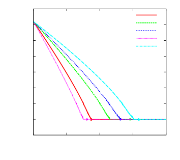
0.50.50.51111.51.51.52222.52.52.53333.53.53.54444.54.54.500100100100200200200300300300400400400θ˙2/nsubscript˙𝜃2𝑛\dot{\theta}_{2}/nt𝑡t[yr]Refer to captionID 1ID 2ID 3ID 4ID 5
(a)
0.50.50.51111.51.51.52222.52.52.53333.53.53.54444.54.54.500100100100200200200300300300400400400θ˙2/nsubscript˙𝜃2𝑛\dot{\theta}_{2}/nt𝑡t[yr]Refer to captionID 6ID 7ID 8ID 9ID 10ID 11ID 12
(b)
Figure 2: Normalized spin rate of the planet vs. time as resulted from the first set of numerical simulations (2(a)) and from the second one (2(b)).

The third set of numerical simulations consist only of an integration setting of e=0.1𝑒0.1e=0.1. It can be noted in Fig. 3 that the planet is trapped in the 3:2 spin-orbit resonance as can be expected from Fig. 4, where we plot the angular acceleration of the planet due to the secular terms of the tidal torque vs. its normalized spin rate (Makarov & Efroimsky, 2013). In that figure, the solid blue line (which correspond to e=0.1𝑒0.1e=0.1) crosses the horizontal reference axis near θ˙2/n=1.5subscript˙𝜃2𝑛1.5\dot{\theta}_{2}/n=1.5. This is the reason why we pointed out in Sect. 1 that eccentricity plays a key role in the possibility of capture in higher-than-synchronous resonances. This observation is in agreement with the results obtained by Noyelles et al. (2014).
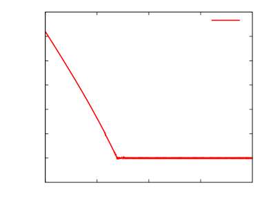
1111.51.51.52222.52.52.53333.53.53.54444.54.54.500100100100200200200300300300400400400θ˙2/nsubscript˙𝜃2𝑛\dot{\theta}_{2}/nt𝑡t[yr]Refer to captionID 13
Figure 3: Normalized spin rate of the planet vs. time as result of the third set of numerical simulations (the one with e=0.1𝑒0.1e=0.1. We obtain the planet’s results captured in the 3:2 spin-orbit resonance.
2.52.5-2.522-21.51.5-1.511-10.50.5-0.5000.50.50.51111.51.51.52222.52.52.50.50.50.51111.51.51.52222.52.52.53333.53.53.5444

θ¨2tide×103superscriptdelimited-⟨⟩subscript¨𝜃2tidesuperscript103\left\langle\ddot{\theta}_{2}\right\rangle^{\mathrm{tide}}\times 10^{3}[day2superscriptday2\mathrm{day}^{-2}]

θ˙2/nsubscript˙𝜃2𝑛\dot{\theta}_{2}/n22-211-10011122211-10.50.5-0.5000.50.50.5111(θ˙2/n1)×104subscript˙𝜃2𝑛1superscript104\left(\dot{\theta}_{2}/n-1\right)\times 10^{4}0.50.5-0.50.40.4-0.40.30.3-0.30.20.2-0.20.10.1-0.1000.10.10.10.20.20.211-10.50.5-0.5000.50.50.5111(θ˙2/n1.5)×105subscript˙𝜃2𝑛1.5superscript105\left(\dot{\theta}_{2}/n-1.5\right)\times 10^{5}Refer to captione=0.02𝑒0.02e=0.02e=0.1𝑒0.1e=0.1
Figure 4: Angular acceleration of the planet due to the secular terms of the tidal torque vs. its normalized spin rate for two values of the eccentricity, the current e=0.02𝑒0.02e=0.02 and e=0.1𝑒0.1e=0.1. We zoomed in on two neighborhoods around the 1:1 and 3:2 spin-orbit resonances for clarity.

In Fig. 4 we also may find a justification of this choice in the initial value of the planet’s spin rate (i.e., θ˙2=4.1nsubscript˙𝜃24.1𝑛\dot{\theta}_{2}=4.1\,n). As can be noted in the aforementioned figure, the angular acceleration of the planet – due to the secular terms of the tidal torque – is practically constant for θ˙2/n4subscript˙𝜃2𝑛4\dot{\theta}_{2}/n\geq 4 and thus, if we consider higher initial values of the planet’s spin rate, the only difference would be that the latter ends up reaching the 1:1 spin-orbit resonance some time later.

Now, we shift the focus to the orbital evolution of the Kepler-21 system. As a general observation, it can be noted that the major semiaxis and the eccentricity evolved in time in a similar way in each simulation when compared to the others, only differing in the final value of the corresponding time rates, as noted in Figs 5 and 6. This similarity can be understood by examining Fig. 7, where we can verify that the system behaves as expected from the same figure, provided that the planet’s rotational evolutionary timescale is much shorter than the orbital one. In this sense, we can know in advance how the system is expected to evolve over time before performing any numerical integration. In the case of Kepler-21, we see that the major semiaxis, the eccentricity, and the obliquity grow in time up to the 1:1 spin-orbit resonance and then start decreasing. This result is also consistent with Noyelles et al. (2014), who found that Mercury’s spin evolved so swiftly that the planet got trapped in its end-state only some 10-20 million of years after its accretion.
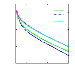
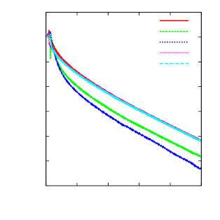
1212-121010-1088-866-644-422-20022200200020002000400040004000600060006000800080008000100001000010000

(aa0)×107𝑎subscript𝑎0superscript107\left(a-a_{0}\right)\times 10^{7}[AU]

t𝑡t[yr]Refer to captionID 1ID 2ID 3ID 4ID 5
(a)
1212-121010-1088-866-644-422-20022200200020002000400040004000600060006000800080008000100001000010000

(ee0)×104𝑒subscript𝑒0superscript104\left(e-e_{0}\right)\times 10^{4}

t𝑡t[yr]Refer to captionID 1ID 2ID 3ID 4ID 5
(b)
Figure 5: Time evolution of aa0𝑎subscript𝑎0a-a_{0}, ee0𝑒subscript𝑒0e-e_{0} (where a0subscript𝑎0a_{0} and e0subscript𝑒0e_{0} are the initial values of the major semiaxis and the eccentricity, respectively) as the result of the first set of numerical simulations, i.e., those varying the rheological parameters of the planet.
99-988-877-766-655-544-433-322-211-10011100200020002000400040004000600060006000800080008000100001000010000

(aa0)×107𝑎subscript𝑎0superscript107\left(a-a_{0}\right)\times 10^{7}[AU]

t𝑡t[yr]Refer to captionID 6ID 7ID 8ID 9ID 10ID 11ID 12
(a)
1010-1099-988-877-766-655-544-433-322-211-10011100200020002000400040004000600060006000800080008000100001000010000

(ee0)×104𝑒subscript𝑒0superscript104\left(e-e_{0}\right)\times 10^{4}

t𝑡t[yr]Refer to captionID 6ID 7ID 8ID 9ID 10ID 11ID 12
(b)
Figure 6: Time evolution of aa0𝑎subscript𝑎0a-a_{0}, ee0𝑒subscript𝑒0e-e_{0} (where a0subscript𝑎0a_{0} and e0subscript𝑒0e_{0} are the initial values of the major semiaxis and the eccentricity, respectively) as result from the second set of numerical simulations, i.e., those varying the dynamical parameters J2subscript𝐽2J_{2} and (BA)/C2𝐵𝐴subscript𝐶2(B-A)/C_{2} of the planet.
33-322-211-1001112223330.50.50.51111.51.51.52222.52.52.53333.53.53.544433-322-211-10011122233311-10.50.5-0.5000.50.50.51110.050.050.050.10.10.10.150.150.1511-10.50.5-0.5000.50.50.5111Refer to captionθ˙2/nsubscript˙𝜃2𝑛\dot{\theta}_{2}/ndadt×108delimited-⟨⟩d𝑎d𝑡superscript108\left\langle\frac{\mathrm{d}a}{\mathrm{d}t}\right\rangle\times 10^{8}[AUyr1AUsuperscriptyr1\mathrm{AU}\,\mathrm{yr}^{-1}]dedt×105delimited-⟨⟩d𝑒d𝑡superscript105\left\langle\frac{\mathrm{d}e}{\mathrm{d}t}\right\rangle\times 10^{5}[yr1superscriptyr1\mathrm{yr}^{-1}]di2dt×102delimited-⟨⟩dsubscript𝑖2d𝑡superscript102\left\langle\frac{\mathrm{d}i_{2}}{\mathrm{d}t}\right\rangle\times 10^{2}[°yr1°superscriptyr1\degr\mathrm{yr}^{-1}](θ˙2/n1)×104subscript˙𝜃2𝑛1superscript104\left(\dot{\theta}_{2}/n-1\right)\times 10^{4}(θ˙2/n1.5)×104subscript˙𝜃2𝑛1.5superscript104\left(\dot{\theta}_{2}/n-1.5\right)\times 10^{4}
Figure 7: Time derivatives of a𝑎a, e,𝑒e, and i2subscript𝑖2i_{2} due to the secular terms of the disturbing function vs. the normalized spin rate of the planet obtained by direct evaluation of the corresponding equations of motion.

Perhaps it would be interesting to see the individual contributions of the tidal potentials of the star and of the planet onto the dynamics of the system that they are both a part of. In Figs. 8(a) and 8(b), we show the time derivatives of the major semiaxis and of the eccentricity, respectively, due to the secular terms of the star’s tidal potential, labeled with superscript (1), and to the planet’s tidal potential, labeled with a superscript (2). It can be observed that in both cases, the star’s contribution is approximately four orders of magnitude weaker than that of the planet’s.
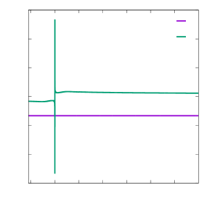
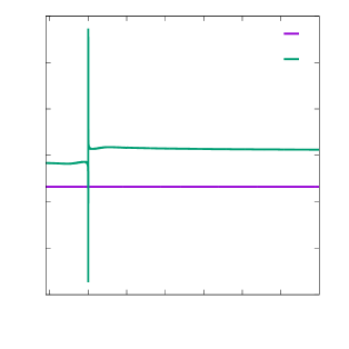
33-322-211-1001112223330.50.50.51111.51.51.52222.52.52.53333.53.53.5444Refer to captionθ˙2/nsubscript˙𝜃2𝑛\dot{\theta}_{2}/ndadt(1)×1011superscriptdelimited-⟨⟩d𝑎d𝑡1superscript1011\left\langle\frac{\mathrm{d}a}{\mathrm{d}t}\right\rangle^{(1)}\times 10^{11}[AUyr1AUsuperscriptyr1\mathrm{AU}\,\mathrm{yr}^{-1}]dadt(2)×108superscriptdelimited-⟨⟩d𝑎d𝑡2superscript108\left\langle\frac{\mathrm{d}a}{\mathrm{d}t}\right\rangle^{(2)}\times 10^{8}[AUyr1AUsuperscriptyr1\mathrm{AU}\,\mathrm{yr}^{-1}]
(a)
33-322-211-1001112223330.50.50.51111.51.51.52222.52.52.53333.53.53.5444Refer to captionθ˙2/nsubscript˙𝜃2𝑛\dot{\theta}_{2}/ndedt(1)×108superscriptdelimited-⟨⟩d𝑒d𝑡1superscript108\left\langle\frac{\mathrm{d}e}{\mathrm{d}t}\right\rangle^{(1)}\times 10^{8}[yr1superscriptyr1\mathrm{yr}^{-1}]dedt(2)×105superscriptdelimited-⟨⟩d𝑒d𝑡2superscript105\left\langle\frac{\mathrm{d}e}{\mathrm{d}t}\right\rangle^{(2)}\times 10^{5}[yr1superscriptyr1\mathrm{yr}^{-1}]
(b)
Figure 8: Time derivatives of the major semiaxis (8(a)) and the eccentricity (8(b)) as a function of the normalized spin rate of the planet. In this figure, the contributions of the secular terms of the tidal potentials generated by the star and the planet are shown separately.

Concerning the time evolution of the inclination (i1subscript𝑖1i_{1}), we obtained a seemingly counter-intuitive result, provided that its time derivative has a positive value of about 1.35×10¹⁰°yr11.35superscript1010°superscriptyr11.35\times 10^{-10}\,\degr\,\mbox{yr}^{-1}, which is practically independent of the planet’s normalized spin rate. This implies that

Gm1m2aC1θ˙1>nξ𝐺subscript𝑚1subscript𝑚2𝑎subscript𝐶1subscript˙𝜃1𝑛𝜉\frac{G\,m_{1}\,m_{2}}{a\,C_{1}\,\dot{\theta}_{1}}>\frac{n}{\xi}

for the case of the Kepler-21 system, as can be noted from Eqs. (64d) and (63). As we can also note in Eq. (64d), the time evolution of i1subscript𝑖1i_{1} depends only on the stellar parameters. Thus, the time derivative of the orbital inclination can be plotted against the normalized spin rate of the star, as shown in Fig. 9, where we consider two different values of the stellar viscosity. From Table 3 we can verify that θ˙1/n<1subscript˙𝜃1𝑛1\dot{\theta}_{1}/n<1 and, as a consequence, the time derivative of i1subscript𝑖1i_{1} is inevitably positive by virtue of the dynamical model developed in this work.
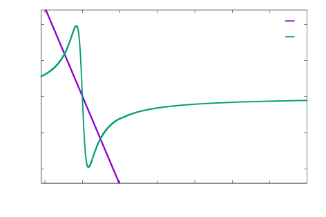
11-10.50.5-0.5000.50.50.51110.50.50.51111.51.51.52222.52.52.53333.53.53.5444Refer to captionθ˙1/nsubscript˙𝜃1𝑛\dot{\theta}_{1}/ndi1dt×1011delimited-⟨⟩dsubscript𝑖1d𝑡superscript1011\left\langle\frac{\mathrm{d}i_{1}}{\mathrm{d}t}\right\rangle\times 10^{11}[°yr1°superscriptyr1\degr\,\mathrm{yr}^{-1}]; η1=1012subscript𝜂1superscript1012\eta_{1}=10^{12}di1dt×106delimited-⟨⟩dsubscript𝑖1d𝑡superscript106\left\langle\frac{\mathrm{d}i_{1}}{\mathrm{d}t}\right\rangle\times 10^{6}[°yr1°superscriptyr1\degr\,\mathrm{yr}^{-1}]; η1=1018subscript𝜂1superscript1018\eta_{1}=10^{18}
Figure 9: Time derivatives of i1subscript𝑖1i_{1} vs. the normalized spin rate of the planet obtained by direct evaluation of Eq. (64d), considering two different values of the stellar viscosity.

With respect to the obliquity (i2subscript𝑖2i_{2}), it begins to decrease exponentially after the planet gets trapped in the synchronous rotation, as can be observed in Figs. 10(a) and 10(b). By virtue of Fig. 7, we can also know in advance the general behavior of the time evolution of the obliquity, at least qualitatively as in the case of the major semiaxis and the eccentricity discussed before.
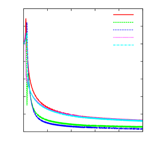
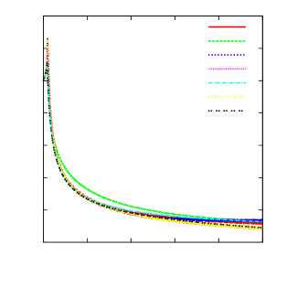
0011122233344455566677700200020002000400040004000600060006000800080008000100001000010000

i2subscript𝑖2i_{2}[°°\degr]

t𝑡t[yr]Refer to captionID 1ID 2ID 3ID 4ID 5
(a)
0011122233344455566677700200020002000400040004000600060006000800080008000100001000010000

i2subscript𝑖2i_{2}[°°\degr]

t𝑡t[yr]Refer to captionID 6ID 7ID 8ID 9ID 10ID 11ID 12
(b)
Figure 10: Time evolution of the planet’s obliquity (i2subscript𝑖2i_{2}) as result from the first (10(a)) – those varying the rheological parameters – and second (10(b)) – i.e. those varying the dynamical parameters – the set of numerical simulations.

It may seem that in Fig. 7 the time derivatives of the major semiaxis, the eccentricity, and the obliquity are equal to zero when the planet is trapped in the 1:1 spin-orbit resonance but, as seen in Figs. 5, 6, and 10, these orbital elements decrease in time after the planet has reached the synchronous rotation. There are two reasons behind this fact. On one hand, as pointed out before, the synchronism is not exact. On the other hand, if we take a look at a very narrow interval around the 1:1 spin orbit resonance in Fig. 7, as shown in Fig. 11, we note that the time derivatives of a𝑎a, e𝑒e and i2subscript𝑖2i_{2} are not exactly zero for θ˙2=nsubscript˙𝜃2𝑛\dot{\theta}_{2}=n.

0.040.04-0.040.030.03-0.030.020.02-0.020.010.01-0.01000.010.010.0144-433-322-211-100111222333444Refer to caption(θ˙2/n1)×108subscript˙𝜃2𝑛1superscript108\left(\dot{\theta}_{2}/n-1\right)\times 10^{8}dadt×108delimited-⟨⟩d𝑎d𝑡superscript108\left\langle\frac{\mathrm{d}a}{\mathrm{d}t}\right\rangle\times 10^{8}[AUyr1AUsuperscriptyr1\mathrm{AU}\,\mathrm{yr}^{-1}]dedt×106delimited-⟨⟩d𝑒d𝑡superscript106\left\langle\frac{\mathrm{d}e}{\mathrm{d}t}\right\rangle\times 10^{6}[yr1superscriptyr1\mathrm{yr}^{-1}]di2dt×103delimited-⟨⟩dsubscript𝑖2d𝑡superscript103\left\langle\frac{\mathrm{d}i_{2}}{\mathrm{d}t}\right\rangle\times 10^{3}[°yr1°superscriptyr1\degr\mathrm{yr}^{-1}]
Figure 11: Again, the time derivatives of a𝑎a, e,𝑒e, and i2subscript𝑖2i_{2} due to the secular terms of the disturbing function vs. the normalized spin rate of the planet obtained by direct evaluation of the corresponding equations of motion but in a narrow interval around the 1:1 spin-orbit resonance.

As a final comment on the numerical simulations, it should be noted that this kind of problem involves different timescales of the dynamical evolution. As noted in Figs. 12 and 13(a), the time rates of the mean anomaly at the epoch, the argument of pericenter, and the longitude of the ascending node, both defined on the stellar equator, are on the order of 104superscript10410^{-4}; while the apsidal and nodal precessions as seen from the planet are on the order of 101superscript10110^{1}102superscript10210^{2} (Fig. 13(b)). Then it is necessary for the numerical integration scheme to treat these timescales separately.

Taking into account that n4.8×104°yr1𝑛4.8superscript104°superscriptyr1n\approx 4.8\times 10^{4}{}\degr\mbox{yr}^{-1}, as well, we then have that M˙n˙𝑀𝑛\dot{M}\approx n and, in consequence, we consider a time step of 103Porbsuperscript103subscript𝑃orb10^{-3}P_{\mathrm{orb}} (ΔtfastΔsubscript𝑡fast\Delta t_{\mathrm{fast}}) to integrate θ2subscript𝜃2\theta_{2}, M𝑀M, ω2subscript𝜔2\omega_{2}, and Ω2subscriptΩ2\Omega_{2}, and a time step of one year (ΔtslowΔsubscript𝑡slow\Delta t_{\mathrm{slow}}) for the rest of the dynamical parameters, that is, a𝑎a, e𝑒e, i1subscript𝑖1i_{1} and i2subscript𝑖2i_{2}.

The dynamical variables were integrated together but in different stages within the numerical integration scheme in order to implement the separation of the fast-varying and the slow-varying variables described before. More specifically, the former were integrated using fourth-order Runge-Kutta method (ΔtslowΔsubscript𝑡slow\Delta t_{\mathrm{slow}}), while the latter were integrated using the Bulirsch-Stoer method (Press et al., 1992) with the corresponding time step ΔtfastΔsubscript𝑡fast\Delta t_{\mathrm{fast}}.

The aforementioned integration scheme starts with an evaluation of the time derivatives of the slow-varying variables at the beginning of the integration interval, that is, the first stage of the Runge-Kutta method, for example, at tisubscript𝑡𝑖t_{i}. Then the fast-varying variables are integrated using the Bulirsch-Stoer method up to ti+Δtslow/2.subscript𝑡𝑖Δsubscript𝑡slow2t_{i}+\Delta t_{\mathrm{slow}}/2. At that point, the second stage of the Runge-Kutta method is performed with the updated value of the planet’s spin rate in order to evaluate properly the tidal frequencies and the time derivatives of the slow-varying variables. Immediately, the fast-varying variables are integrated again up to the end of the integration interval, that is, ti+Δtslowsubscript𝑡𝑖Δsubscript𝑡slowt_{i}+\Delta t_{\mathrm{slow}} where the new value of θ˙2subscript˙𝜃2\dot{\theta}_{2} is taken to compute the new values of both the tidal frequencies and the slow-varying variables’ time derivatives. Finally, the last stage of the Runge-Kutta method is carried out in order to compute the new values of the slow-varying variables; these are used to start the integration on the next interval together with the last computed values of the planet’s spin rate and the rest of the fast-varying variables.
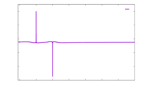
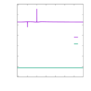
0.30.3-0.30.20.2-0.20.10.1-0.1000.10.10.10.20.20.20.50.50.51111.51.51.52222.52.52.53333.53.53.5444Refer to captionθ˙2/nsubscript˙𝜃2𝑛\dot{\theta}_{2}/ndM0dt×103delimited-⟨⟩dsubscript𝑀0d𝑡superscript103\left\langle\frac{\mathrm{d}M_{0}}{\mathrm{d}t}\right\rangle\times 10^{3}[°yr1°superscriptyr1\degr\mathrm{yr}^{-1}]
Figure 12: Time derivative of the mean anomaly at the epoch vs. the normalized spin rat of the planet.
0.40.4-0.40.20.2-0.2000.20.20.20.40.40.40.60.60.60.80.80.81110.50.50.51111.51.51.52222.52.52.53333.53.53.5444Refer to captionθ˙2/nsubscript˙𝜃2𝑛\dot{\theta}_{2}/ndω1dt×103delimited-⟨⟩dsubscript𝜔1d𝑡superscript103\left\langle\frac{\mathrm{d\omega_{1}}}{\mathrm{d}t}\right\rangle\times 10^{3}[°yr1°superscriptyr1\degr\mathrm{yr}^{-1}]dΩ1dt×103delimited-⟨⟩dsubscriptΩ1d𝑡superscript103\left\langle\frac{\mathrm{d}\Omega_{1}}{\mathrm{d}t}\right\rangle\times 10^{3}[°yr1°superscriptyr1\degr\mathrm{yr}^{-1}]
(a)
2525-252020-201515-151010-1055-5005551010101515152020202525250.50.50.51111.51.51.52222.52.52.53333.53.53.5444Refer to captionθ˙2/nsubscript˙𝜃2𝑛\dot{\theta}_{2}/ndω2dt×101delimited-⟨⟩dsubscript𝜔2d𝑡superscript101\left\langle\frac{\mathrm{d}\omega_{2}}{\mathrm{d}t}\right\rangle\times 10^{-1}[°yr1°superscriptyr1\degr\mathrm{yr}^{-1}]dΩ2dt×101delimited-⟨⟩dsubscriptΩ2d𝑡superscript101\left\langle\frac{\mathrm{d}\Omega_{2}}{\mathrm{d}t}\right\rangle\times 10^{-1}[°yr1°superscriptyr1\degr\mathrm{yr}^{-1}]
(b)
Figure 13: Time rate of the apsidal and nodal precession, as seen from the star (13(a)) and from the planet (13(b)), vs. the normalized spin rate of the planet.

5.2 Timescales of orbital decay and circularization

In general terms, we define the characteristic timescale of the evolution of an orbital element as that which is required for a certain change in that element to take place. Since the orbital inclination and the obliquity of the planet evolve in the way described earlier in this work, we only consider the timescales that correspond to the major semiaxis and the eccentricity. Mathematically expressed, the characteristic timescale of the former, τasubscript𝜏𝑎\tau_{a}, and the latter, τesubscript𝜏𝑒\tau_{e}, are defined as:

τa=(rRochea)(dadt)1,subscript𝜏𝑎subscript𝑟Roche𝑎superscriptd𝑎d𝑡1\tau_{a}=\left(r_{\mathrm{Roche}}-a\right)\left(\frac{\mathrm{d}a}{\mathrm{d}t}\right)^{-1}, (76)
τe=e(dedt)1,subscript𝜏𝑒𝑒superscriptd𝑒d𝑡1\tau_{e}=-\,e\left(\frac{\mathrm{d}e}{\mathrm{d}t}\right)^{-1}, (77)

where rRochesubscript𝑟Rocher_{\mathrm{Roche}} is the Roche limit and the values of a𝑎a and e𝑒e are the current ones. It can be noted that τasubscript𝜏𝑎\tau_{a} correspond to the time interval that elapses from the current value of a𝑎a up to the planet reaches the Roche radius, beyond which it would be completely destroyed by tidal forces. The latter is defined as (Murray & Dermott, 1999):

rRoche=Rp(3msmp)13.subscript𝑟Rochesubscript𝑅psuperscript3subscript𝑚ssubscript𝑚p13r_{\mathrm{Roche}}=R_{\mathrm{p}}\left(3\frac{m_{\mathrm{s}}}{m_{\mathrm{p}}}\right)^{\frac{1}{3}}. (78)

Of course, this definition does not take into account the rigidity of the material that compose the body but only considers self-gravity. Even so, it can be considered as an upper limit. For the Kepler-21 system, rRoche4.54×103subscript𝑟Roche4.54superscript103r_{\mathrm{Roche}}\approx 4.54\times 10^{-3} au.

Table 5: Orbital decay and eccentricity damping timescales of the Kepler-21 system obtained through Eqs. (76) and (77) by evaluating the corresponding equation of motion at θ˙2/n=1subscript˙𝜃2𝑛1\dot{\theta}_{2}/n=1 for different values of the rheological parameters and the eccentricity.
e𝑒e τMsubscript𝜏𝑀\tau_{M} [yr] α𝛼\alpha τasubscript𝜏𝑎\tau_{a} [×106absentsuperscript106\times 10^{6} yr] τesubscript𝜏𝑒\tau_{e} [×106absentsuperscript106\times 10^{6} yr]
0.010.010.01 101010 0.20.20.2 751.32751.32751.32 0.1010.1010.101
0.020.020.02 101010 0.20.20.2 629.23629.23629.23 0.3450.3450.345
0.020.020.02 505050 0.20.20.2 662.78662.78662.78 0.3610.3610.361
0.020.020.02 100100100 0.20.20.2 675.81675.81675.81 0.3670.3670.367
0.020.020.02 101010 0.150.150.15 617.57617.57617.57 0.3390.3390.339
0.020.020.02 101010 0.30.30.3 679.20679.20679.20 0.3680.3680.368
0.10.10.1 101010 0.20.20.2 98.95598.95598.955 1.5421.5421.542

Replacing in Eqs. (76) and (77) the corresponding values given in Table 3 and that of dadtdelimited-⟨⟩d𝑎d𝑡\left\langle\frac{\mathrm{d}a}{\mathrm{d}t}\right\rangle and dedtdelimited-⟨⟩d𝑒d𝑡\left\langle\frac{\mathrm{d}e}{\mathrm{d}t}\right\rangle from Eqs. (64a) and (64b) evaluated at θ˙2=nsubscript˙𝜃2𝑛\dot{\theta}_{2}=n for different values of the rheological parameters, we obtain the values of orbital decay and circularization timescales. The results are shown in Table 5 together with the corresponding values of the rheological parameters. As can be observed in that table, since the orbital decay timescale is much larger than the others, when arRoche𝑎subscript𝑟Rochea\approx r_{\mathrm{Roche}}, the orbit will be completely circularized.

5.3 Possibility of detecting tidal effects

It may be an interesting exercise to consider the possibility of contrasting the results obtained from numerical simulation with those from observations. Within the limits of this work, we can answer the question of whether tidal effects can be detected only in part. In recent years, great advances have been made in observational techniques that allow for highly precise measurements of the physical and orbital parameters of planets orbiting stars other than the Sun. One of these quantities is the orbital period, Porbsubscript𝑃orbP_{\mathrm{orb}}, of planets, which can be measured by observing several successive transits and is defined by:

Porb=2πn.subscript𝑃orb2𝜋𝑛P_{\mathrm{orb}}=\frac{2\,\pi}{n}. (79)

If we assume that the orbital parameters of a two body system evolve in time only due to the tides each body rises on the other – as was supposed in the last subsection – then the orbital period is also expected to evolve as a consequence of the time variation of the major semiaxis. This can be expressed mathematically as:

dPorbdt=2πn2dndt.dsubscript𝑃orbd𝑡2𝜋superscript𝑛2d𝑛d𝑡\frac{\mathrm{d}P_{\mathrm{orb}}}{\mathrm{d}t}=-\frac{2\,\pi}{n^{2}}\frac{\mathrm{d}n}{\mathrm{d}t}. (80)

From Eq. (1), we have:

dndt=32nadadt.d𝑛d𝑡32𝑛𝑎d𝑎d𝑡\frac{\mathrm{d}n}{\mathrm{d}t}=-\frac{3}{2}\frac{n}{a}\frac{\mathrm{d}a}{\mathrm{d}t}.

Then, Eq. (80) can be rewritten as:

dPorbdt=3πnadadt.dsubscript𝑃orbd𝑡3𝜋𝑛𝑎d𝑎d𝑡\frac{\mathrm{d}P_{\mathrm{orb}}}{\mathrm{d}t}=\frac{3\,\pi}{n\,a}\frac{\mathrm{d}a}{\mathrm{d}t}. (81)

If we take the values of the parameters for the Kepler 21 system given in Table 3, compute n𝑛n with Eq. (1), and also take the value of dadtdelimited-⟨⟩d𝑎d𝑡\left\langle\frac{\mathrm{d}a}{\mathrm{d}t}\right\rangle, obtained from direct evaluation of Eq. (64a), assuming θ˙2=nsubscript˙𝜃2𝑛\dot{\theta}_{2}=n and evaluating the tidal frequencies with Eq. (17), and then we replace them in Eq. (81), we get the following result:

dPorbdttide0.003879syr,superscriptdelimited-⟨⟩dsubscript𝑃orbd𝑡tide0.003879syr\left\langle\frac{\mathrm{d}P_{\mathrm{orb}}}{\mathrm{d}t}\right\rangle^{\mathrm{tide}}\approx-0.003879\,\frac{\mathrm{s}}{\mathrm{yr}},

which is equivalent to a decrement of nearly 3.88ms3.88ms3.88\,\mbox{ms} per year. As a consequence, we would need more than 1000 years to measure a difference of about 4 seconds. The measured orbital period of planet Kepler-21b is 2.785782.785782.78578 days with an uncertainty of 0.000030.000030.00003 days (López-Morales et al., 2016), which is equivalent to approximately 2.6s2.6s2.6\,\mbox{s}. This result clearly shows the impossibility of detecting tidal effects, if simply by measuring the orbital period of the planet, at least in this case.

In this regard, the question of whether it is possible to detect tidal effects by measuring the orbital period of certain exoplanets has motivated the publication of several recent works. Depending on each particular case, some authors conclude that it is not possible to detect tidal effect, as in Petrucci et al. (2019), and others not only assert that they measure a decrease of the orbital period, but also that it is a consequence of the orbital decay due to tidal interaction (Yee et al., 2019).

6 Final discussion and conclusions

In this work, we develop an accurate method for studying the dynamical evolution of a binary system formed by a rocky planet and its host star. We follow the work by Boué & Efroimsky (2019) to obtain a set of equations of motion which, on one hand, describe the secular time evolution of the orbital elements attributed to the secular terms of the tidal potentials of both partners and the secular terms related to the J2subscript𝐽2J_{2} coefficient. On the other hand, it gives the time rate of the stellar spin rate due to the secular terms of the corresponding tidal torque and the time evolution of the proper rotation angle of the planet due to the combined action of the secular terms of the tidal torque and the periodic terms of the triaxiality-induced torque. Thus, the main results of this investigation are: Eqs. (64a), (64b), (64c), (64d), (64e), (64f), (64g), (64h), (64i), (65a), and (65b) which contain no singularities in the limit of vanishing eccentricities, inclination, and obliquity. Bearing in mind that the transformation introduced to obtain the equations only moves the latter singularity to e=1𝑒1e=1 and i=90°𝑖90°i=90\degr, we would like to stress the fact that it is a convenient substitution because it allows for the possibility that the eccentricity and the inclinations reach very low values (even zero) without affecting the stability of the numerical integration.

As a case study, we chose the Kepler-21 system. We find that the commonly accepted approximate expression of the tidal modes, given by Eq. (17), could no longer be valid in studies such as that carried out in this paper. In other words, at least in the case of the Kepler-21 system, the apsidal and nodal precessions induced by tides and the J2subscript𝐽2J_{2}-related terms is appreciable. Also, we find that the time of tidal synchronization strongly depends on the values of the rheological parameters, as is shown in Fig. 2(a).

Regarding the rotational state of planet Kepler-21b, even though it could be or have previously been trapped in the 3:2 spin-orbit resonance, we expect that it has already reached the synchronous rotation, not only because this is its most likely state, but as it orbits very close to a massive star with a radius nearly twice grater than that of our Sun, we can reasonably suppose that the planet is undergoing a strong internal dissipation which can cause an increase of its internal temperature with the consequent decrease of the viscosity and of the Maxwell time. As explained by Makarov et al. (2018), this decrease of the Maxwell time can cause the escape from higher-than-synchronous rotation states in a time interval shorter that the corresponding decrease of the corresponding capture probabilities due to the decrease of the eccentricity in time (Makarov, 2015).

It worth mentioning that from the point of view of tidal theory, the case of Kepler-21 – after the planet has reached the synchronous rotation – is analogous to the case of Phobos, which is gradually spiraling inwards towards Mars (Efroimsky & Lainey, 2007). In this sense, the timescales of orbital decay and circularization given in Table 5 are upper bounds, that is, the rates of orbital decay and circularization become greater as the planet approaches its host star. Even though the results shown in Table 5 suggest that the planet has a short time to exist, we can note that the more rapidly the eccentricity gets damped, the more the time it takes the planet to reach the Roche limit.

The time evolution of the orbital inclination (i1subscript𝑖1i_{1}) seems to be counter-intuitive. However, this is a particularity of the Kepler-21 system, but there could be other systems in which a more “expectable” conclusion is reached. As shown in Subsect. 5.1, tidal interaction can lead the major semiaxis, the eccentricity, and the inclinations to increase or decrease over time, depending on the particular combinations of the values of the rheological and dynamical parameters and variables involved (see Veras et al., 2019).

We would like to emphasize that even though we have addressed the study of a particular system, the formalism developed in this work is equally applicable to other analogous systems, formed by a star and a terrestrial planet. Moreover, this methodology could be adapted to model the dynamical evolution of binary asteroids. We will carry out the former and the latter types of studies in future works.

The analytical model that we propose in this work takes into account the tidal dissipation of both components of a binary system and the influence of both the J2subscript𝐽2J_{2}-related secular terms in the orbital evolution and the permanent-triaxiality-induced torque in the rotational evolution of one of the bodies, while the rotational evolution of the other is considered to be dominated only by the tidal interaction. We are aware that there are other effects that could be equally important to the dynamical evolution and could later be incorporated into the formalism, such as the oblateness of the star, General Relativity (Correia et al., 2011), dynamical tides in the star (Bolmont & Mathis, 2016; Hodžić et al., 2018), atmospheric tides in the planet (Correia & Laskar, 2003; Leconte et al., 2015), magnetic couplings between the star and the planet (Ahuir et al., 2019), and stellar evolution (Benbakoura et al., 2019).

Acknowledgements.
We acknowledge the funding from ANPCyT through PICT 1144-13 and CONICET through PIP 699-15. This investigation was supported by the institutional cluster HOPE at IAFE (http://www.iafe.uba.ar/HOPE/), where all the numerical simulations were performed, and by the SAO/NASA Astrophysics Data System. Santiago Luna wants to acknowledge the fruitful discussions with Michael Efroimsky, Gwenaël Boué, Dimitri Veras and Valeri Makarov, which helped to reach a better understanding of the dynamical evolution near spin-orbit resonances and to improve the quality of this work. This research has made use of the NASA Exoplanet Archive, which is operated by the California Institute of Technology, under contract with the National Aeronautics and Space Administration under the Exoplanet Exploration Program.

References

  • Ahuir et al. (2019) Ahuir, J., Strugarek, A., Brun, A.-S., et al. 2019, arXiv e-prints, arXiv:1912.06867
  • Benbakoura et al. (2019) Benbakoura, M., Réville, V., Brun, A. S., Le Poncin-Lafitte, C., & Mathis, S. 2019, A&A, 621, A124
  • Bolmont & Mathis (2016) Bolmont, E. & Mathis, S. 2016, Celestial Mechanics and Dynamical Astronomy, 126, 275
  • Boué et al. (2016) Boué, G., Correia, A. C. M., & Laskar, J. 2016, Celestial Mechanics and Dynamical Astronomy, 126, 31
  • Boué & Efroimsky (2019) Boué, G. & Efroimsky, M. 2019, Celestial Mechanics and Dynamical Astronomy, 131, 30
  • Brouwer & Clemence (1961) Brouwer, D. & Clemence, G. M. 1961, Methods of Celestial Mechanics (Academic Press)
  • Correia et al. (2014) Correia, A. C. M., Boué, G., Laskar, J., & Rodríguez, A. 2014, A&A, 571, A50
  • Correia & Laskar (2003) Correia, A. C. M. & Laskar, J. 2003, Journal of Geophysical Research: Planets, 108
  • Correia et al. (2011) Correia, A. C. M., Laskar, J., Farago, F., & Boué, G. 2011, Celestial Mechanics and Dynamical Astronomy, 111, 105
  • Efroimsky (2005a) Efroimsky, M. 2005a, Annals of the New York Academy of Sciences, 1065, 346
  • Efroimsky (2005b) Efroimsky, M. 2005b, Celestial Mechanics and Dynamical Astronomy, 91, 75
  • Efroimsky (2012) Efroimsky, M. 2012, Celestial Mechanics and Dynamical Astronomy, 112, 283
  • Efroimsky (2015) Efroimsky, M. 2015, The Astronomical Journal, 150, 98
  • Efroimsky & Goldreich (2004) Efroimsky, M. & Goldreich, P. 2004, A&A, 415, 1187
  • Efroimsky & Lainey (2007) Efroimsky, M. & Lainey, V. 2007, Journal of Geophysical Research (Planets), 112, E12003
  • Efroimsky & Makarov (2013) Efroimsky, M. & Makarov, V. V. 2013, The Astrophysical Journal, 764, 26
  • Efroimsky & Williams (2009) Efroimsky, M. & Williams, J. G. 2009, Celestial Mechanics and Dynamical Astronomy, 104, 257
  • Frouard & Efroimsky (2017) Frouard, J. & Efroimsky, M. 2017, Celestial Mechanics and Dynamical Astronomy, 129, 177
  • Frouard & Efroimsky (2018) Frouard, J. & Efroimsky, M. 2018, Monthly Notices of the Royal Astronomical Society, 473, 728
  • Giacaglia (1976) Giacaglia, G. E. O. 1976, Celestial Mechanics, 14, 515
  • Goldreich & Peale (1966) Goldreich, P. & Peale, S. 1966, The Astronomical Journal, 71, 425
  • Gooding & Wagner (2008) Gooding, R. H. & Wagner, C. A. 2008, Celestial Mechanics and Dynamical Astronomy, 101, 247
  • Hodžić et al. (2018) Hodžić, V., Triaud, A. H. M. J., Anderson, D. R., et al. 2018, Monthly Notices of the Royal Astronomical Society, 481, 5091
  • Howell et al. (2012) Howell, S. B., Rowe, J. F., Bryson, S. T., et al. 2012, The Astrophysical Journal, 746, 123
  • Hughes (1981) Hughes, S. 1981, Celestial Mechanics, 25, 101
  • Kaula (1961) Kaula, W. M. 1961, Geophysical Journal, 5, 104
  • Kaula (2000) Kaula, W. M. 2000, Theory of Satellite Geodesy: Applications of Satellites to Geodesy, Dover Earth Science Series (Dover Publications)
  • Kopeikin et al. (2011) Kopeikin, S., Efroimsky, M., & Kaplan, G. 2011, Relativistic Celestial Mechanics of the Solar System (Wiley-VCH)
  • Leconte et al. (2015) Leconte, J., Wu, H., Menou, K., & Murray, N. 2015, Science, 347, 632
  • López-Morales et al. (2016) López-Morales, M., Haywood, R. D., Coughlin, J. L., et al. 2016, The Astronomical Journal, 152, 204
  • Makarov (2012) Makarov, V. V. 2012, The Astrophysical Journal, 752, 73
  • Makarov (2015) Makarov, V. V. 2015, The Astrophysical Journal, 810, 12
  • Makarov et al. (2012) Makarov, V. V., Berghea, C., & Efroimsky, M. 2012, The Astrophysical Journal, 761, 83
  • Makarov et al. (2018) Makarov, V. V., Berghea, C. T., & Efroimsky, M. 2018, The Astrophysical Journal, 857, 142
  • Makarov & Efroimsky (2013) Makarov, V. V. & Efroimsky, M. 2013, ApJ, 764, 27
  • Mignard (1979) Mignard, F. 1979, Moon and Planets, 20, 301
  • Mignard (1980) Mignard, F. 1980, Moon and Planets, 23, 185
  • Miguel & Brunini (2010) Miguel, Y. & Brunini, A. 2010, Monthly Notices of the Royal Astronomical Society, 406, 1935
  • Murray & Dermott (1999) Murray, C. D. & Dermott, S. F. 1999, Solar system dynamics (Cambridge University Press)
  • Noyelles et al. (2014) Noyelles, B., Frouard, J., Makarov, V. V., & Efroimsky, M. 2014, Icarus, 241, 26
  • Petrucci et al. (2019) Petrucci, R., Jofré, E., Gómez, Y., et al. 2019, Monthly Notices of the Royal Astronomical Society, 491, 1243
  • Press et al. (1992) Press, W., Flannery, B., Teukolsky, S., & Vetterling, W. 1992, Numerical Recipes in FORTRAN 77: Volume 1, Volume 1 of Fortran Numerical Recipes: The Art of Scientific Computing (Cambridge University Press)
  • Proulx & McClain (1988) Proulx, R. J. & McClain, W. D. 1988, Journal of Guidance, Control, and Dynamics, 11, 313
  • Renaud & Henning (2018) Renaud, J. P. & Henning, W. G. 2018, The Astrophysical Journal, 857, 98
  • Rodríguez et al. (2012) Rodríguez, A., Callegari, N., J., Michtchenko, T. A., & Hussmann, H. 2012, Monthly Notices of the Royal Astronomical Society, 427, 2239
  • Seager (2010) Seager, S. 2010, Exoplanet Atmospheres: Physical Processes, Princeton Series in Astrophysics (Princeton University Press)
  • Shoji & Kurita (2014) Shoji, D. & Kurita, K. 2014, The Astrophysical Journal, 789, 3
  • Stamenković et al. (2012) Stamenković, V., Noack, L., Breuer, D., & Spohn, T. 2012, The Astrophysical Journal, 748, 41
  • Sundberg & Cooper (2010) Sundberg, M. & Cooper, R. F. 2010, Philosophical Magazine, 90, 2817
  • Torge & Müller (2012) Torge, W. & Müller, J. 2012, Geodesy, 4th edn. (Walter de Gruyter)
  • Valencia et al. (2006) Valencia, D., O’Connell, R. J., & Sasselov, D. 2006, Icarus, 181, 545
  • Valencia et al. (2007a) Valencia, D., Sasselov, D. D., & O’Connell, R. J. 2007a, The Astrophysical Journal, 665, 1413
  • Valencia et al. (2007b) Valencia, D., Sasselov, D. D., & O’Connell, R. J. 2007b, The Astrophysical Journal, 656, 545
  • Veras et al. (2019) Veras, D., Efroimsky, M., Makarov, V. V., et al. 2019, Monthly Notices of the Royal Astronomical Society, 486, 3831
  • Yee et al. (2019) Yee, S. W., Winn, J. N., Knutson, H. A., et al. 2019, The Astrophysical Journal, 888, L5
  • Zeng & Jacobsen (2017) Zeng, L. & Jacobsen, S. B. 2017, The Astrophysical Journal, 837, 164

Appendix A Expression of the sums of adimensional terms of the derivatives of the disturbing potentials

In the following, we give the complete expressions of the derivatives of the disturbing potentials considered in this work. Regarding the gradient of the tidal potentials of both bodies, we also give the secular terms of the corresponding derivatives. The latter is identified by the superscript ”(sec)”. Among the aforementioned expressions, the terms corresponding to (lmpq)=(201q)𝑙𝑚𝑝𝑞201𝑞(lmpq)=(201q) and (lmpq)=(220q)𝑙𝑚𝑝𝑞220𝑞(lmpq)=(220q) are shown, in particular. As earlier in this work, such terms are identified with the respective subscripts.

A.1 Major semiaxis

Ulmpqhs(k)a=l=2m=0lp=0lq=h=0ls=(l+1)(Rka)2l+1(lm)!(l+m)!(2δ0m)Flmp(ik)Glpq(e)Flmh(ik)Glhs(e)×[cos(vlmpq(k)vlmhs(k))KR(k)(l,χlmpq(k))+sin(vlmpq(k)vlmhs(k))KI(k)(l,χlmpq(k))],superscriptsubscript𝑈𝑙𝑚𝑝𝑞𝑠𝑘𝑎superscriptsubscript𝑙2superscriptsubscript𝑚0𝑙superscriptsubscript𝑝0𝑙superscriptsubscript𝑞superscriptsubscript0𝑙superscriptsubscript𝑠𝑙1superscriptsubscript𝑅𝑘𝑎2𝑙1𝑙𝑚𝑙𝑚2subscript𝛿0𝑚subscript𝐹𝑙𝑚𝑝subscript𝑖𝑘subscript𝐺𝑙𝑝𝑞𝑒subscript𝐹𝑙𝑚subscript𝑖𝑘subscript𝐺𝑙𝑠𝑒delimited-[]superscriptsubscript𝑣𝑙𝑚𝑝𝑞𝑘superscriptsubscript𝑣𝑙𝑚𝑠𝑘superscriptsubscript𝐾R𝑘𝑙superscriptsubscript𝜒𝑙𝑚𝑝𝑞𝑘superscriptsubscript𝑣𝑙𝑚𝑝𝑞𝑘superscriptsubscript𝑣𝑙𝑚𝑠𝑘superscriptsubscript𝐾I𝑘𝑙superscriptsubscript𝜒𝑙𝑚𝑝𝑞𝑘\frac{\partial U_{lmpqhs}^{(k)}}{\partial a}=\sum_{l=2}^{\infty}\sum_{m=0}^{l}\sum_{p=0}^{l}\sum_{q=-\infty}^{\infty}\sum_{h=0}^{l}\sum_{s=-\infty}^{\infty}(l+1)\left(\frac{R_{k}}{a}\right)^{2l+1}\frac{(l-m)!}{(l+m)!}(2-\delta_{0m})F_{lmp}(i_{k})\,G_{lpq}(e)\,F_{lmh}(i_{k})\,G_{lhs}(e)\\ \times\left[\cos\left(v_{lmpq}^{(k)}-v_{lmhs}^{(k)}\right)K_{\mathrm{R}}^{(k)}\left(l,\chi_{lmpq}^{(k)}\right)+\sin\left(v_{lmpq}^{(k)}-v_{lmhs}^{(k)}\right)K_{\mathrm{I}}^{(k)}\left(l,\chi_{lmpq}^{(k)}\right)\right], (82a)
Ulmpq(k)a=l=2m=0lp=0lq=(l+1)(Rka)2l+1(lm)!(l+m)!(2δ0m)Flmp2(ik)Glpq2(e)KR(k)(l,χlmpq(k)),delimited-⟨⟩superscriptsubscript𝑈𝑙𝑚𝑝𝑞𝑘𝑎superscriptsubscript𝑙2superscriptsubscript𝑚0𝑙superscriptsubscript𝑝0𝑙superscriptsubscript𝑞𝑙1superscriptsubscript𝑅𝑘𝑎2𝑙1𝑙𝑚𝑙𝑚2subscript𝛿0𝑚superscriptsubscript𝐹𝑙𝑚𝑝2subscript𝑖𝑘superscriptsubscript𝐺𝑙𝑝𝑞2𝑒superscriptsubscript𝐾R𝑘𝑙superscriptsubscript𝜒𝑙𝑚𝑝𝑞𝑘\left\langle\frac{\partial U_{lmpq}^{(k)}}{\partial a}\right\rangle=\sum_{l=2}^{\infty}\sum_{m=0}^{l}\sum_{p=0}^{l}\sum_{q=-\infty}^{\infty}(l+1)\left(\frac{R_{k}}{a}\right)^{2l+1}\frac{(l-m)!}{(l+m)!}(2-\delta_{0m})F_{lmp}^{2}(i_{k})\,G_{lpq}^{2}(e)\,K_{\mathrm{R}}^{(k)}\left(l,\chi_{lmpq}^{(k)}\right), (82b)
U201q(k)a=3(Rka)5F2012(ik)q=G21q2(e)KR(k)(2,ω201q(k)),delimited-⟨⟩superscriptsubscript𝑈201𝑞𝑘𝑎3superscriptsubscript𝑅𝑘𝑎5superscriptsubscript𝐹2012subscript𝑖𝑘superscriptsubscript𝑞superscriptsubscript𝐺21𝑞2𝑒superscriptsubscript𝐾R𝑘2superscriptsubscript𝜔201𝑞𝑘\left\langle\frac{\partial U_{201q}^{(k)}}{\partial a}\right\rangle=3\left(\frac{R_{k}}{a}\right)^{5}F_{201}^{2}(i_{k})\sum_{q=-\infty}^{\infty}G_{21q}^{2}(e)\,K_{\mathrm{R}}^{(k)}\left(2,\omega_{201q}^{(k)}\right), (82c)
U220q(k)a=14(Rka)5F2202(ik)q=G20q2(e)KR(k)(2,ω220q(k)),delimited-⟨⟩superscriptsubscript𝑈220𝑞𝑘𝑎14superscriptsubscript𝑅𝑘𝑎5superscriptsubscript𝐹2202subscript𝑖𝑘superscriptsubscript𝑞superscriptsubscript𝐺20𝑞2𝑒superscriptsubscript𝐾R𝑘2superscriptsubscript𝜔220𝑞𝑘\left\langle\frac{\partial U_{220q}^{(k)}}{\partial a}\right\rangle=\frac{1}{4}\left(\frac{R_{k}}{a}\right)^{5}F_{220}^{2}(i_{k})\sum_{q=-\infty}^{\infty}G_{20q}^{2}(e)\,K_{\mathrm{R}}^{(k)}\left(2,\omega_{220q}^{(k)}\right), (82d)
Vlmpq(2)a=l=2m=0lp=0lq=(l+1)(R2a)lFlmp(i2)Glpq(e)[Clmcos(vlmpq(2)mθ2+ϕlm)+Slmsin(vlmpq(2)mθ2+ϕlm)],superscriptsubscript𝑉𝑙𝑚𝑝𝑞2𝑎superscriptsubscript𝑙2superscriptsubscript𝑚0𝑙superscriptsubscript𝑝0𝑙superscriptsubscript𝑞𝑙1superscriptsubscript𝑅2𝑎𝑙subscript𝐹𝑙𝑚𝑝subscript𝑖2subscript𝐺𝑙𝑝𝑞𝑒delimited-[]subscript𝐶𝑙𝑚superscriptsubscript𝑣𝑙𝑚𝑝𝑞2𝑚subscript𝜃2subscriptitalic-ϕ𝑙𝑚subscript𝑆𝑙𝑚superscriptsubscript𝑣𝑙𝑚𝑝𝑞2𝑚subscript𝜃2subscriptitalic-ϕ𝑙𝑚\frac{\partial V_{lmpq}^{(2)}}{\partial a}=\sum_{l=2}^{\infty}\sum_{m=0}^{l}\sum_{p=0}^{l}\sum_{q=-\infty}^{\infty}(l+1)\left(\frac{R_{2}}{a}\right)^{l}F_{lmp}(i_{2})\,G_{lpq}(e)\left[C_{lm}\cos\left(v_{lmpq}^{(2)}-m\,\theta_{2}+\phi_{lm}\right)+S_{lm}\sin\left(v_{lmpq}^{(2)}-m\,\theta_{2}+\phi_{lm}\right)\right], (82e)
V201q(2)a=3J2(R2a)2F201(i2)q=G21q(e)cos(qM),superscriptsubscript𝑉201𝑞2𝑎3subscript𝐽2superscriptsubscript𝑅2𝑎2subscript𝐹201subscript𝑖2superscriptsubscript𝑞subscript𝐺21𝑞𝑒𝑞𝑀\frac{\partial V_{201q}^{(2)}}{\partial a}=-3J_{2}\left(\frac{R_{2}}{a}\right)^{2}F_{201}(i_{2})\sum_{q=-\infty}^{\infty}G_{21q}(e)\cos(q\,M), (82f)
V220q(2)a=34(BA)m2a2F220(i2)q=G20q(e)cos[2(ω2+Ω2θ2)+(2+q)M].superscriptsubscript𝑉220𝑞2𝑎34𝐵𝐴subscript𝑚2superscript𝑎2subscript𝐹220subscript𝑖2superscriptsubscript𝑞subscript𝐺20𝑞𝑒2subscript𝜔2subscriptΩ2subscript𝜃22𝑞𝑀\frac{\partial V_{220q}^{(2)}}{\partial a}=\frac{3}{4}\frac{(B-A)}{m_{2}\,a^{2}}F_{220}(i_{2})\sum_{q=-\infty}^{\infty}G_{20q}(e)\cos\left[2\left(\omega_{2}+\Omega_{2}-\theta_{2}\right)+(2+q)M\right]. (82g)

A.2 Eccentricity

Ulmpqhs(k)e=l=2m=0lp=0lq=h=0ls=(Rka)2l+1(lm)!(l+m)!(2δ0m)Flmp(ik)Glpq(e)Flmh(ik)dGlhs(e)de×[cos(vlmpq(k)vlmhs(k))KR(k)(l,χlmpq(k))+sin(vlmpq(k)vlmhs(k))KI(k)(l,χlmpq(k))],superscriptsubscript𝑈𝑙𝑚𝑝𝑞𝑠𝑘𝑒superscriptsubscript𝑙2superscriptsubscript𝑚0𝑙superscriptsubscript𝑝0𝑙superscriptsubscript𝑞superscriptsubscript0𝑙superscriptsubscript𝑠superscriptsubscript𝑅𝑘𝑎2𝑙1𝑙𝑚𝑙𝑚2subscript𝛿0𝑚subscript𝐹𝑙𝑚𝑝subscript𝑖𝑘subscript𝐺𝑙𝑝𝑞𝑒subscript𝐹𝑙𝑚subscript𝑖𝑘dsubscript𝐺𝑙𝑠𝑒d𝑒delimited-[]superscriptsubscript𝑣𝑙𝑚𝑝𝑞𝑘superscriptsubscript𝑣𝑙𝑚𝑠𝑘superscriptsubscript𝐾R𝑘𝑙superscriptsubscript𝜒𝑙𝑚𝑝𝑞𝑘superscriptsubscript𝑣𝑙𝑚𝑝𝑞𝑘superscriptsubscript𝑣𝑙𝑚𝑠𝑘superscriptsubscript𝐾I𝑘𝑙superscriptsubscript𝜒𝑙𝑚𝑝𝑞𝑘\frac{\partial U_{lmpqhs}^{(k)}}{\partial e}=\sum_{l=2}^{\infty}\sum_{m=0}^{l}\sum_{p=0}^{l}\sum_{q=-\infty}^{\infty}\sum_{h=0}^{l}\sum_{s=-\infty}^{\infty}\left(\frac{R_{k}}{a}\right)^{2l+1}\frac{(l-m)!}{(l+m)!}(2-\delta_{0m})F_{lmp}(i_{k})\,G_{lpq}(e)\,F_{lmh}(i_{k})\,\frac{\mathrm{d}G_{lhs}(e)}{\mathrm{d}e}\\ \times\left[\cos\left(v_{lmpq}^{(k)}-v_{lmhs}^{(k)}\right)K_{\mathrm{R}}^{(k)}\left(l,\chi_{lmpq}^{(k)}\right)+\sin\left(v_{lmpq}^{(k)}-v_{lmhs}^{(k)}\right)K_{\mathrm{I}}^{(k)}\left(l,\chi_{lmpq}^{(k)}\right)\right], (83a)
Ulmpq(k)e=l=2m=0lp=0lq=(Rka)2l+1(lm)!(l+m)!(2δ0m)Flmp2(ik)Glpq(e)dGlpq(e)deKR(k)(l,χlmpq(k)),delimited-⟨⟩superscriptsubscript𝑈𝑙𝑚𝑝𝑞𝑘𝑒superscriptsubscript𝑙2superscriptsubscript𝑚0𝑙superscriptsubscript𝑝0𝑙superscriptsubscript𝑞superscriptsubscript𝑅𝑘𝑎2𝑙1𝑙𝑚𝑙𝑚2subscript𝛿0𝑚superscriptsubscript𝐹𝑙𝑚𝑝2subscript𝑖𝑘subscript𝐺𝑙𝑝𝑞𝑒dsubscript𝐺𝑙𝑝𝑞𝑒d𝑒superscriptsubscript𝐾R𝑘𝑙superscriptsubscript𝜒𝑙𝑚𝑝𝑞𝑘\left\langle\frac{\partial U_{lmpq}^{(k)}}{\partial e}\right\rangle=\sum_{l=2}^{\infty}\sum_{m=0}^{l}\sum_{p=0}^{l}\sum_{q=-\infty}^{\infty}\left(\frac{R_{k}}{a}\right)^{2l+1}\frac{(l-m)!}{(l+m)!}(2-\delta_{0m})F_{lmp}^{2}(i_{k})\,G_{lpq}(e)\frac{\mathrm{d}G_{lpq}(e)}{\mathrm{d}e}\,K_{\mathrm{R}}^{(k)}\left(l,\chi_{lmpq}^{(k)}\right), (83b)
U201q(k)e=(Rka)5F2012(ik)q=G21q(e)dG21q(e)deKR(k)(2,ω201q(k)),delimited-⟨⟩superscriptsubscript𝑈201𝑞𝑘𝑒superscriptsubscript𝑅𝑘𝑎5superscriptsubscript𝐹2012subscript𝑖𝑘superscriptsubscript𝑞subscript𝐺21𝑞𝑒dsubscript𝐺21𝑞𝑒d𝑒superscriptsubscript𝐾R𝑘2superscriptsubscript𝜔201𝑞𝑘\left\langle\frac{\partial U_{201q}^{(k)}}{\partial e}\right\rangle=\left(\frac{R_{k}}{a}\right)^{5}F_{201}^{2}(i_{k})\sum_{q=-\infty}^{\infty}G_{21q}(e)\frac{\mathrm{d}G_{21q}(e)}{\mathrm{d}e}\,K_{\mathrm{R}}^{(k)}\left(2,\omega_{201q}^{(k)}\right), (83c)
U220q(k)e=112(Rka)5F2202(ik)q=G20q(e)dG20q(e)deKR(k)(2,ω220q(k)),delimited-⟨⟩superscriptsubscript𝑈220𝑞𝑘𝑒112superscriptsubscript𝑅𝑘𝑎5superscriptsubscript𝐹2202subscript𝑖𝑘superscriptsubscript𝑞subscript𝐺20𝑞𝑒dsubscript𝐺20𝑞𝑒d𝑒superscriptsubscript𝐾R𝑘2superscriptsubscript𝜔220𝑞𝑘\left\langle\frac{\partial U_{220q}^{(k)}}{\partial e}\right\rangle=\frac{1}{12}\left(\frac{R_{k}}{a}\right)^{5}F_{220}^{2}(i_{k})\sum_{q=-\infty}^{\infty}G_{20q}(e)\frac{\mathrm{d}G_{20q}(e)}{\mathrm{d}e}\,K_{\mathrm{R}}^{(k)}\left(2,\omega_{220q}^{(k)}\right), (83d)
Vlmpq(2)e=l=2m=0lp=0lq=(R2a)lFlmp(i2)dGlpq(e)de[Clmcos(vlmpq(2)mθ2+ϕlm)+Slmsin(vlmpq(2)mθ2+ϕlm)],superscriptsubscript𝑉𝑙𝑚𝑝𝑞2𝑒superscriptsubscript𝑙2superscriptsubscript𝑚0𝑙superscriptsubscript𝑝0𝑙superscriptsubscript𝑞superscriptsubscript𝑅2𝑎𝑙subscript𝐹𝑙𝑚𝑝subscript𝑖2dsubscript𝐺𝑙𝑝𝑞𝑒d𝑒delimited-[]subscript𝐶𝑙𝑚superscriptsubscript𝑣𝑙𝑚𝑝𝑞2𝑚subscript𝜃2subscriptitalic-ϕ𝑙𝑚subscript𝑆𝑙𝑚superscriptsubscript𝑣𝑙𝑚𝑝𝑞2𝑚subscript𝜃2subscriptitalic-ϕ𝑙𝑚\frac{\partial V_{lmpq}^{(2)}}{\partial e}=\sum_{l=2}^{\infty}\sum_{m=0}^{l}\sum_{p=0}^{l}\sum_{q=-\infty}^{\infty}\left(\frac{R_{2}}{a}\right)^{l}F_{lmp}(i_{2})\,\frac{\mathrm{d}G_{lpq}(e)}{\mathrm{d}e}\left[C_{lm}\cos\left(v_{lmpq}^{(2)}-m\,\theta_{2}+\phi_{lm}\right)+S_{lm}\sin\left(v_{lmpq}^{(2)}-m\,\theta_{2}+\phi_{lm}\right)\right], (83e)
V201q(2)e=J2(R2a)2F201(i2)q=dG21q(e)decos(qM),superscriptsubscript𝑉201𝑞2𝑒subscript𝐽2superscriptsubscript𝑅2𝑎2subscript𝐹201subscript𝑖2superscriptsubscript𝑞dsubscript𝐺21𝑞𝑒d𝑒𝑞𝑀\frac{\partial V_{201q}^{(2)}}{\partial e}=-J_{2}\left(\frac{R_{2}}{a}\right)^{2}F_{201}(i_{2})\sum_{q=-\infty}^{\infty}\frac{\mathrm{d}G_{21q}(e)}{\mathrm{d}e}\cos(q\,M), (83f)
V220q(2)e=14(BA)m2a2F220(i2)q=dG20q(e)decos[2(ω2+Ω2θ2)+(2+q)M].superscriptsubscript𝑉220𝑞2𝑒14𝐵𝐴subscript𝑚2superscript𝑎2subscript𝐹220subscript𝑖2superscriptsubscript𝑞dsubscript𝐺20𝑞𝑒d𝑒2subscript𝜔2subscriptΩ2subscript𝜃22𝑞𝑀\frac{\partial V_{220q}^{(2)}}{\partial e}=\frac{1}{4}\frac{(B-A)}{m_{2}\,a^{2}}F_{220}(i_{2})\sum_{q=-\infty}^{\infty}\frac{\mathrm{d}G_{20q}(e)}{\mathrm{d}e}\cos\left[2\left(\omega_{2}+\Omega_{2}-\theta_{2}\right)+(2+q)M\right]. (83g)

A.3 Mean anomaly

Ulmpqhs(k)M=l=2m=0lp=0lq=h=0ls=(Rka)2l+1(lm)!(l+m)!(2δ0m)Flmp(ik)Glpq(e)Flmh(ik)Glhs(e)×[sin(vlmpq(k)vlmhs(k))KR(k)(l,χlmpq(k))cos(vlmpq(k)vlmhs(k))KI(k)(l,χlmpq(k))](l2h+s),superscriptsubscript𝑈𝑙𝑚𝑝𝑞𝑠𝑘𝑀superscriptsubscript𝑙2superscriptsubscript𝑚0𝑙superscriptsubscript𝑝0𝑙superscriptsubscript𝑞superscriptsubscript0𝑙superscriptsubscript𝑠superscriptsubscript𝑅𝑘𝑎2𝑙1𝑙𝑚𝑙𝑚2subscript𝛿0𝑚subscript𝐹𝑙𝑚𝑝subscript𝑖𝑘subscript𝐺𝑙𝑝𝑞𝑒subscript𝐹𝑙𝑚subscript𝑖𝑘subscript𝐺𝑙𝑠𝑒delimited-[]superscriptsubscript𝑣𝑙𝑚𝑝𝑞𝑘superscriptsubscript𝑣𝑙𝑚𝑠𝑘superscriptsubscript𝐾R𝑘𝑙superscriptsubscript𝜒𝑙𝑚𝑝𝑞𝑘superscriptsubscript𝑣𝑙𝑚𝑝𝑞𝑘superscriptsubscript𝑣𝑙𝑚𝑠𝑘superscriptsubscript𝐾I𝑘𝑙superscriptsubscript𝜒𝑙𝑚𝑝𝑞𝑘𝑙2𝑠\frac{\partial U_{lmpqhs}^{(k)}}{\partial M}=\sum_{l=2}^{\infty}\sum_{m=0}^{l}\sum_{p=0}^{l}\sum_{q=-\infty}^{\infty}\sum_{h=0}^{l}\sum_{s=-\infty}^{\infty}\left(\frac{R_{k}}{a}\right)^{2l+1}\frac{(l-m)!}{(l+m)!}(2-\delta_{0m})F_{lmp}(i_{k})\,G_{lpq}(e)\,F_{lmh}(i_{k})\,G_{lhs}(e)\\ \times\left[\sin\left(v_{lmpq}^{(k)}-v_{lmhs}^{(k)}\right)K_{\mathrm{R}}^{(k)}\left(l,\chi_{lmpq}^{(k)}\right)-\cos\left(v_{lmpq}^{(k)}-v_{lmhs}^{(k)}\right)K_{\mathrm{I}}^{(k)}\left(l,\chi_{lmpq}^{(k)}\right)\right](l-2h+s), (84a)
Ulmpq(k)M=l=2m=0lp=0lq=(Rka)2l+1(lm)!(l+m)!(2δ0m)Flmp2(ik)Glpq2(e)KI(k)(l,χlmpq(k))(l2p+q).delimited-⟨⟩superscriptsubscript𝑈𝑙𝑚𝑝𝑞𝑘𝑀superscriptsubscript𝑙2superscriptsubscript𝑚0𝑙superscriptsubscript𝑝0𝑙superscriptsubscript𝑞superscriptsubscript𝑅𝑘𝑎2𝑙1𝑙𝑚𝑙𝑚2subscript𝛿0𝑚superscriptsubscript𝐹𝑙𝑚𝑝2subscript𝑖𝑘superscriptsubscript𝐺𝑙𝑝𝑞2𝑒superscriptsubscript𝐾I𝑘𝑙superscriptsubscript𝜒𝑙𝑚𝑝𝑞𝑘𝑙2𝑝𝑞\left\langle\frac{\partial U_{lmpq}^{(k)}}{\partial M}\right\rangle=-\sum_{l=2}^{\infty}\sum_{m=0}^{l}\sum_{p=0}^{l}\sum_{q=-\infty}^{\infty}\left(\frac{R_{k}}{a}\right)^{2l+1}\frac{(l-m)!}{(l+m)!}(2-\delta_{0m})F_{lmp}^{2}(i_{k})\,G_{lpq}^{2}(e)\,K_{\mathrm{I}}^{(k)}\left(l,\chi_{lmpq}^{(k)}\right)(l-2p+q). (84b)
U201q(k)M=(Rka)5F2012(ik)q=G21q2(e)qKI(k)(2,ω201q(k)),delimited-⟨⟩superscriptsubscript𝑈201𝑞𝑘𝑀superscriptsubscript𝑅𝑘𝑎5superscriptsubscript𝐹2012subscript𝑖𝑘superscriptsubscript𝑞superscriptsubscript𝐺21𝑞2𝑒𝑞superscriptsubscript𝐾I𝑘2superscriptsubscript𝜔201𝑞𝑘\left\langle\frac{\partial U_{201q}^{(k)}}{\partial M}\right\rangle=-\left(\frac{R_{k}}{a}\right)^{5}F_{201}^{2}(i_{k})\sum_{q=-\infty}^{\infty}G_{21q}^{2}(e)\,q\,K_{\mathrm{I}}^{(k)}\left(2,\omega_{201q}^{(k)}\right), (84c)
U220q(k)M=112(Rka)5F2202(ik)q=G20q2(e)(2+q)KI(k)(2,ω220q(k)),delimited-⟨⟩superscriptsubscript𝑈220𝑞𝑘𝑀112superscriptsubscript𝑅𝑘𝑎5superscriptsubscript𝐹2202subscript𝑖𝑘superscriptsubscript𝑞superscriptsubscript𝐺20𝑞2𝑒2𝑞superscriptsubscript𝐾I𝑘2superscriptsubscript𝜔220𝑞𝑘\left\langle\frac{\partial U_{220q}^{(k)}}{\partial M}\right\rangle=-\frac{1}{12}\left(\frac{R_{k}}{a}\right)^{5}F_{220}^{2}(i_{k})\sum_{q=-\infty}^{\infty}G_{20q}^{2}(e)\,(2+q)\,K_{\mathrm{I}}^{(k)}\left(2,\omega_{220q}^{(k)}\right), (84d)
Vlmpq(2)M=l=2m=0lp=0lq=(R2a)lFlmp(i2)Glpq(e)[Clmsin(vlmpq(2)mθ2+ϕlm)+Slmcos(vlmpq(2)mθ2+ϕlm)](l2p+q),superscriptsubscript𝑉𝑙𝑚𝑝𝑞2𝑀superscriptsubscript𝑙2superscriptsubscript𝑚0𝑙superscriptsubscript𝑝0𝑙superscriptsubscript𝑞superscriptsubscript𝑅2𝑎𝑙subscript𝐹𝑙𝑚𝑝subscript𝑖2subscript𝐺𝑙𝑝𝑞𝑒delimited-[]subscript𝐶𝑙𝑚superscriptsubscript𝑣𝑙𝑚𝑝𝑞2𝑚subscript𝜃2subscriptitalic-ϕ𝑙𝑚subscript𝑆𝑙𝑚superscriptsubscript𝑣𝑙𝑚𝑝𝑞2𝑚subscript𝜃2subscriptitalic-ϕ𝑙𝑚𝑙2𝑝𝑞\frac{\partial V_{lmpq}^{(2)}}{\partial M}=\sum_{l=2}^{\infty}\sum_{m=0}^{l}\sum_{p=0}^{l}\sum_{q=-\infty}^{\infty}\left(\frac{R_{2}}{a}\right)^{l}F_{lmp}(i_{2})\,G_{lpq}(e)\left[-C_{lm}\sin\left(v_{lmpq}^{(2)}-m\,\theta_{2}+\phi_{lm}\right)+S_{lm}\cos\left(v_{lmpq}^{(2)}-m\,\theta_{2}+\phi_{lm}\right)\right](l-2p+q), (84e)
V201q(2)M=J2(R2a)2F201(i2)q=G21q(e)qsin(qM),superscriptsubscript𝑉201𝑞2𝑀subscript𝐽2superscriptsubscript𝑅2𝑎2subscript𝐹201subscript𝑖2superscriptsubscript𝑞subscript𝐺21𝑞𝑒𝑞𝑞𝑀\frac{\partial V_{201q}^{(2)}}{\partial M}=J_{2}\left(\frac{R_{2}}{a}\right)^{2}F_{201}(i_{2})\sum_{q=-\infty}^{\infty}G_{21q}(e)\,q\,\sin(q\,M), (84f)
V220q(2)M=14(BA)m2a2F220(i2)q=G20q(e)(2+q)sin[2(ω2+Ω2θ2)+(2+q)M].superscriptsubscript𝑉220𝑞2𝑀14𝐵𝐴subscript𝑚2superscript𝑎2subscript𝐹220subscript𝑖2superscriptsubscript𝑞subscript𝐺20𝑞𝑒2𝑞2subscript𝜔2subscriptΩ2subscript𝜃22𝑞𝑀\frac{\partial V_{220q}^{(2)}}{\partial M}=-\frac{1}{4}\frac{(B-A)}{m_{2}\,a^{2}}F_{220}(i_{2})\sum_{q=-\infty}^{\infty}G_{20q}(e)\,(2+q)\,\sin\left[2(\omega_{2}+\Omega_{2}-\theta_{2})+(2+q)\,M\right]. (84g)

A.4 Inclination with respect to the star’s and planet’s equators

Ulmpqhs(k)ik=l=2m=0lp=0lq=h=0ls=(Rka)2l+1(lm)!(l+m)!(2δ0m)Flmp(ik)Glpq(e)dFlmh(ik)dikGlhs(e)×[cos(vlmpq(k)vlmhs(k))KR(k)(l,χlmpq(k))+sin(vlmpq(k)vlmhs(k))KI(k)(l,χlmpq(k))],superscriptsubscript𝑈𝑙𝑚𝑝𝑞𝑠𝑘subscript𝑖𝑘superscriptsubscript𝑙2superscriptsubscript𝑚0𝑙superscriptsubscript𝑝0𝑙superscriptsubscript𝑞superscriptsubscript0𝑙superscriptsubscript𝑠superscriptsubscript𝑅𝑘𝑎2𝑙1𝑙𝑚𝑙𝑚2subscript𝛿0𝑚subscript𝐹𝑙𝑚𝑝subscript𝑖𝑘subscript𝐺𝑙𝑝𝑞𝑒dsubscript𝐹𝑙𝑚subscript𝑖𝑘dsubscript𝑖𝑘subscript𝐺𝑙𝑠𝑒delimited-[]superscriptsubscript𝑣𝑙𝑚𝑝𝑞𝑘superscriptsubscript𝑣𝑙𝑚𝑠𝑘superscriptsubscript𝐾R𝑘𝑙superscriptsubscript𝜒𝑙𝑚𝑝𝑞𝑘superscriptsubscript𝑣𝑙𝑚𝑝𝑞𝑘superscriptsubscript𝑣𝑙𝑚𝑠𝑘superscriptsubscript𝐾I𝑘𝑙superscriptsubscript𝜒𝑙𝑚𝑝𝑞𝑘\frac{\partial U_{lmpqhs}^{(k)}}{\partial i_{k}}=\sum_{l=2}^{\infty}\sum_{m=0}^{l}\sum_{p=0}^{l}\sum_{q=-\infty}^{\infty}\sum_{h=0}^{l}\sum_{s=-\infty}^{\infty}\left(\frac{R_{k}}{a}\right)^{2l+1}\frac{(l-m)!}{(l+m)!}(2-\delta_{0m})F_{lmp}(i_{k})\,G_{lpq}(e)\,\frac{\mathrm{d}F_{lmh}(i_{k})}{\mathrm{d}i_{k}}\,G_{lhs}(e)\\ \times\left[\cos\left(v_{lmpq}^{(k)}-v_{lmhs}^{(k)}\right)K_{\mathrm{R}}^{(k)}\left(l,\chi_{lmpq}^{(k)}\right)+\sin\left(v_{lmpq}^{(k)}-v_{lmhs}^{(k)}\right)K_{\mathrm{I}}^{(k)}\left(l,\chi_{lmpq}^{(k)}\right)\right], (85a)
Ulmpq(k)ik=l=2m=0lp=0lq=(Rka)2l+1(lm)!(l+m)!(2δ0m)Flmp(ik)dFlmp(ik)dikGlpq2(e)KR(k)(l,χlmpq(k)),delimited-⟨⟩superscriptsubscript𝑈𝑙𝑚𝑝𝑞𝑘subscript𝑖𝑘superscriptsubscript𝑙2superscriptsubscript𝑚0𝑙superscriptsubscript𝑝0𝑙superscriptsubscript𝑞superscriptsubscript𝑅𝑘𝑎2𝑙1𝑙𝑚𝑙𝑚2subscript𝛿0𝑚subscript𝐹𝑙𝑚𝑝subscript𝑖𝑘dsubscript𝐹𝑙𝑚𝑝subscript𝑖𝑘dsubscript𝑖𝑘superscriptsubscript𝐺𝑙𝑝𝑞2𝑒superscriptsubscript𝐾R𝑘𝑙superscriptsubscript𝜒𝑙𝑚𝑝𝑞𝑘\left\langle\frac{\partial U_{lmpq}^{(k)}}{\partial i_{k}}\right\rangle=\sum_{l=2}^{\infty}\sum_{m=0}^{l}\sum_{p=0}^{l}\sum_{q=-\infty}^{\infty}\left(\frac{R_{k}}{a}\right)^{2l+1}\frac{(l-m)!}{(l+m)!}(2-\delta_{0m})F_{lmp}(i_{k})\frac{\mathrm{d}F_{lmp}(i_{k})}{\mathrm{d}i_{k}}\,G_{lpq}^{2}(e)\,K_{\mathrm{R}}^{(k)}\left(l,\chi_{lmpq}^{(k)}\right), (85b)
U201q(k)ik=(Rka)5F201(ik)dF201(ik)dikq=G21q2(e)KR(k)(2,ω201q(k)),delimited-⟨⟩superscriptsubscript𝑈201𝑞𝑘subscript𝑖𝑘superscriptsubscript𝑅𝑘𝑎5subscript𝐹201subscript𝑖𝑘dsubscript𝐹201subscript𝑖𝑘dsubscript𝑖𝑘superscriptsubscript𝑞superscriptsubscript𝐺21𝑞2𝑒superscriptsubscript𝐾R𝑘2superscriptsubscript𝜔201𝑞𝑘\left\langle\frac{\partial U_{201q}^{(k)}}{\partial i_{k}}\right\rangle=\left(\frac{R_{k}}{a}\right)^{5}F_{201}(i_{k})\frac{\mathrm{d}F_{201}(i_{k})}{\mathrm{d}i_{k}}\sum_{q=-\infty}^{\infty}G_{21q}^{2}(e)\,K_{\mathrm{R}}^{(k)}\left(2,\omega_{201q}^{(k)}\right), (85c)
U220q(k)ik=112(Rka)5F220(ik)dF220(ik)dikq=G20q2(e)KR(k)(2,ω220q(k)),delimited-⟨⟩superscriptsubscript𝑈220𝑞𝑘subscript𝑖𝑘112superscriptsubscript𝑅𝑘𝑎5subscript𝐹220subscript𝑖𝑘dsubscript𝐹220subscript𝑖𝑘dsubscript𝑖𝑘superscriptsubscript𝑞superscriptsubscript𝐺20𝑞2𝑒superscriptsubscript𝐾R𝑘2superscriptsubscript𝜔220𝑞𝑘\left\langle\frac{\partial U_{220q}^{(k)}}{\partial i_{k}}\right\rangle=\frac{1}{12}\left(\frac{R_{k}}{a}\right)^{5}F_{220}(i_{k})\frac{\mathrm{d}F_{220}(i_{k})}{\mathrm{d}i_{k}}\sum_{q=-\infty}^{\infty}G_{20q}^{2}(e)\,K_{\mathrm{R}}^{(k)}\left(2,\omega_{220q}^{(k)}\right), (85d)
Vlmpq(2)i2=l=2m=0lp=0lq=(R2a)ldFlmp(i2)di2Glpq(e)[Clmcos(vlmpq(2)mθ2+ϕlm)+Slmsin(vlmpq(2)mθ2+ϕlm)],superscriptsubscript𝑉𝑙𝑚𝑝𝑞2subscript𝑖2superscriptsubscript𝑙2superscriptsubscript𝑚0𝑙superscriptsubscript𝑝0𝑙superscriptsubscript𝑞superscriptsubscript𝑅2𝑎𝑙dsubscript𝐹𝑙𝑚𝑝subscript𝑖2dsubscript𝑖2subscript𝐺𝑙𝑝𝑞𝑒delimited-[]subscript𝐶𝑙𝑚superscriptsubscript𝑣𝑙𝑚𝑝𝑞2𝑚subscript𝜃2subscriptitalic-ϕ𝑙𝑚subscript𝑆𝑙𝑚superscriptsubscript𝑣𝑙𝑚𝑝𝑞2𝑚subscript𝜃2subscriptitalic-ϕ𝑙𝑚\frac{\partial V_{lmpq}^{(2)}}{\partial i_{2}}=\sum_{l=2}^{\infty}\sum_{m=0}^{l}\sum_{p=0}^{l}\sum_{q=-\infty}^{\infty}\left(\frac{R_{2}}{a}\right)^{l}\frac{\mathrm{d}F_{lmp}(i_{2})}{\mathrm{d}i_{2}}\,G_{lpq}(e)\left[C_{lm}\cos\left(v_{lmpq}^{(2)}-m\,\theta_{2}+\phi_{lm}\right)+S_{lm}\sin\left(v_{lmpq}^{(2)}-m\,\theta_{2}+\phi_{lm}\right)\right], (85e)
V201q(2)i2=J2(R2a)2dF201(i2)di2q=G21q(e)cos(qM),superscriptsubscript𝑉201𝑞2subscript𝑖2subscript𝐽2superscriptsubscript𝑅2𝑎2dsubscript𝐹201subscript𝑖2dsubscript𝑖2superscriptsubscript𝑞subscript𝐺21𝑞𝑒𝑞𝑀\frac{\partial V_{201q}^{(2)}}{\partial i_{2}}=-J_{2}\left(\frac{R_{2}}{a}\right)^{2}\frac{\mathrm{d}F_{201}(i_{2})}{\mathrm{d}i_{2}}\sum_{q=-\infty}^{\infty}\,G_{21q}(e)\cos(q\,M), (85f)
V220q(2)i2=14(BA)m2a2dF220(i2)di2q=G20q(e)cos[2(ω2+Ω2θ2)+(2+q)M].superscriptsubscript𝑉220𝑞2subscript𝑖214𝐵𝐴subscript𝑚2superscript𝑎2dsubscript𝐹220subscript𝑖2dsubscript𝑖2superscriptsubscript𝑞subscript𝐺20𝑞𝑒2subscript𝜔2subscriptΩ2subscript𝜃22𝑞𝑀\frac{\partial V_{220q}^{(2)}}{\partial i_{2}}=\frac{1}{4}\frac{(B-A)}{m_{2}\,a^{2}}\frac{\mathrm{d}F_{220}(i_{2})}{\mathrm{d}i_{2}}\sum_{q=-\infty}^{\infty}\,G_{20q}(e)\cos\left[2(\omega_{2}+\Omega_{2}-\theta_{2})+(2+q)M\right]. (85g)

A.5 Argument of pericenter with respect to the star’s and planet’s equators

Ulmpqhs(k)ωk=l=2m=0lp=0lq=h=0ls=(Rka)2l+1(lm)!(l+m)!(2δ0m)Flmp(ik)Glpq(e)Flmh(ik)Glhs(e)×[sin(vlmpq(k)vlmhs(k))KR(k)(l,χlmpq(k))cos(vlmpq(k)vlmhs(k))KI(k)(l,χlmpq(k))](l2h),superscriptsubscript𝑈𝑙𝑚𝑝𝑞𝑠𝑘subscript𝜔𝑘superscriptsubscript𝑙2superscriptsubscript𝑚0𝑙superscriptsubscript𝑝0𝑙superscriptsubscript𝑞superscriptsubscript0𝑙superscriptsubscript𝑠superscriptsubscript𝑅𝑘𝑎2𝑙1𝑙𝑚𝑙𝑚2subscript𝛿0𝑚subscript𝐹𝑙𝑚𝑝subscript𝑖𝑘subscript𝐺𝑙𝑝𝑞𝑒subscript𝐹𝑙𝑚subscript𝑖𝑘subscript𝐺𝑙𝑠𝑒delimited-[]superscriptsubscript𝑣𝑙𝑚𝑝𝑞𝑘superscriptsubscript𝑣𝑙𝑚𝑠𝑘superscriptsubscript𝐾R𝑘𝑙superscriptsubscript𝜒𝑙𝑚𝑝𝑞𝑘superscriptsubscript𝑣𝑙𝑚𝑝𝑞𝑘superscriptsubscript𝑣𝑙𝑚𝑠𝑘superscriptsubscript𝐾I𝑘𝑙superscriptsubscript𝜒𝑙𝑚𝑝𝑞𝑘𝑙2\frac{\partial U_{lmpqhs}^{(k)}}{\partial\omega_{k}}=\sum_{l=2}^{\infty}\sum_{m=0}^{l}\sum_{p=0}^{l}\sum_{q=-\infty}^{\infty}\sum_{h=0}^{l}\sum_{s=-\infty}^{\infty}\left(\frac{R_{k}}{a}\right)^{2l+1}\frac{(l-m)!}{(l+m)!}(2-\delta_{0m})F_{lmp}(i_{k})\,G_{lpq}(e)\,F_{lmh}(i_{k})\,G_{lhs}(e)\\ \times\left[\sin\left(v_{lmpq}^{(k)}-v_{lmhs}^{(k)}\right)K_{\mathrm{R}}^{(k)}\left(l,\chi_{lmpq}^{(k)}\right)-\cos\left(v_{lmpq}^{(k)}-v_{lmhs}^{(k)}\right)K_{\mathrm{I}}^{(k)}\left(l,\chi_{lmpq}^{(k)}\right)\right](l-2h), (86a)
Ulmpq(k)ωk=l=2m=0lp=0lq=(Rka)2l+1(lm)!(l+m)!(2δ0m)Flmp2(ik)Glpq2(e)KI(k)(l,χlmpq(k))(l2p),delimited-⟨⟩superscriptsubscript𝑈𝑙𝑚𝑝𝑞𝑘subscript𝜔𝑘superscriptsubscript𝑙2superscriptsubscript𝑚0𝑙superscriptsubscript𝑝0𝑙superscriptsubscript𝑞superscriptsubscript𝑅𝑘𝑎2𝑙1𝑙𝑚𝑙𝑚2subscript𝛿0𝑚superscriptsubscript𝐹𝑙𝑚𝑝2subscript𝑖𝑘superscriptsubscript𝐺𝑙𝑝𝑞2𝑒superscriptsubscript𝐾I𝑘𝑙superscriptsubscript𝜒𝑙𝑚𝑝𝑞𝑘𝑙2𝑝\left\langle\frac{\partial U_{lmpq}^{(k)}}{\partial\omega_{k}}\right\rangle=-\sum_{l=2}^{\infty}\sum_{m=0}^{l}\sum_{p=0}^{l}\sum_{q=-\infty}^{\infty}\left(\frac{R_{k}}{a}\right)^{2l+1}\frac{(l-m)!}{(l+m)!}(2-\delta_{0m})F_{lmp}^{2}(i_{k})\,G_{lpq}^{2}(e)\,K_{\mathrm{I}}^{(k)}\left(l,\chi_{lmpq}^{(k)}\right)(l-2p), (86b)
U201q(k)ωk=0,delimited-⟨⟩superscriptsubscript𝑈201𝑞𝑘subscript𝜔𝑘0\left\langle\frac{\partial U_{201q}^{(k)}}{\partial\omega_{k}}\right\rangle=0, (86c)
U220q(k)ωk=16(Rka)5F2202(ik)q=G20q2(e)KI(k)(2,ω220q(k)),delimited-⟨⟩superscriptsubscript𝑈220𝑞𝑘subscript𝜔𝑘16superscriptsubscript𝑅𝑘𝑎5superscriptsubscript𝐹2202subscript𝑖𝑘superscriptsubscript𝑞superscriptsubscript𝐺20𝑞2𝑒superscriptsubscript𝐾I𝑘2superscriptsubscript𝜔220𝑞𝑘\left\langle\frac{\partial U_{220q}^{(k)}}{\partial\omega_{k}}\right\rangle=-\frac{1}{6}\left(\frac{R_{k}}{a}\right)^{5}F_{220}^{2}(i_{k})\sum_{q=-\infty}^{\infty}G_{20q}^{2}(e)\,K_{\mathrm{I}}^{(k)}\left(2,\omega_{220q}^{(k)}\right), (86d)
Vlmpq(2)ω2=l=2m=0lp=0lq=(R2a)lFlmp(i2)Glpq(e)[Clmsin(vlmpq(2)mθ2+ϕlm)+Slmcos(vlmpq(2)mθ2+ϕlm)](l2p),superscriptsubscript𝑉𝑙𝑚𝑝𝑞2subscript𝜔2superscriptsubscript𝑙2superscriptsubscript𝑚0𝑙superscriptsubscript𝑝0𝑙superscriptsubscript𝑞superscriptsubscript𝑅2𝑎𝑙subscript𝐹𝑙𝑚𝑝subscript𝑖2subscript𝐺𝑙𝑝𝑞𝑒delimited-[]subscript𝐶𝑙𝑚superscriptsubscript𝑣𝑙𝑚𝑝𝑞2𝑚subscript𝜃2subscriptitalic-ϕ𝑙𝑚subscript𝑆𝑙𝑚superscriptsubscript𝑣𝑙𝑚𝑝𝑞2𝑚subscript𝜃2subscriptitalic-ϕ𝑙𝑚𝑙2𝑝\frac{\partial V_{lmpq}^{(2)}}{\partial\omega_{2}}=\sum_{l=2}^{\infty}\sum_{m=0}^{l}\sum_{p=0}^{l}\sum_{q=-\infty}^{\infty}\left(\frac{R_{2}}{a}\right)^{l}F_{lmp}(i_{2})\,G_{lpq}(e)\left[-C_{lm}\sin\left(v_{lmpq}^{(2)}-m\,\theta_{2}+\phi_{lm}\right)+S_{lm}\cos\left(v_{lmpq}^{(2)}-m\,\theta_{2}+\phi_{lm}\right)\right](l-2p), (86e)
V201q(2)ω2=0,superscriptsubscript𝑉201𝑞2subscript𝜔20\frac{\partial V_{201q}^{(2)}}{\partial\omega_{2}}=0, (86f)
V220q(2)ω2=14(BA)m2a2F220(i2)q=G20q(e)sin[2(ω2+Ω2θ2)+(2+q)M],superscriptsubscript𝑉220𝑞2subscript𝜔214𝐵𝐴subscript𝑚2superscript𝑎2subscript𝐹220subscript𝑖2superscriptsubscript𝑞subscript𝐺20𝑞𝑒2subscript𝜔2subscriptΩ2subscript𝜃22𝑞𝑀\frac{\partial V_{220q}^{(2)}}{\partial\omega_{2}}=-\frac{1}{4}\frac{(B-A)}{m_{2}\,a^{2}}F_{220}(i_{2})\sum_{q=-\infty}^{\infty}G_{20q}(e)\sin\left[2(\omega_{2}+\Omega_{2}-\theta_{2})+(2+q)M\right], (86g)

A.6 Longitude of ascending node with respect to the star’s and planet’s equators

Ulmpqhs(k)Ωk=l=2m=0lp=0lq=h=0ls=(Rka)2l+1m(lm)!(l+m)!(2δ0m)Flmp(ik)Glpq(e)Flmh(ik)Glhs(e)×[sin(vlmpq(k)vlmhs(k))KR(k)(l,χlmpq(k))cos(vlmpq(k)vlmhs(k))KI(k)(l,χlmpq(k))],superscriptsubscript𝑈𝑙𝑚𝑝𝑞𝑠𝑘subscriptΩ𝑘superscriptsubscript𝑙2superscriptsubscript𝑚0𝑙superscriptsubscript𝑝0𝑙superscriptsubscript𝑞superscriptsubscript0𝑙superscriptsubscript𝑠superscriptsubscript𝑅𝑘𝑎2𝑙1𝑚𝑙𝑚𝑙𝑚2subscript𝛿0𝑚subscript𝐹𝑙𝑚𝑝subscript𝑖𝑘subscript𝐺𝑙𝑝𝑞𝑒subscript𝐹𝑙𝑚subscript𝑖𝑘subscript𝐺𝑙𝑠𝑒delimited-[]superscriptsubscript𝑣𝑙𝑚𝑝𝑞𝑘superscriptsubscript𝑣𝑙𝑚𝑠𝑘superscriptsubscript𝐾R𝑘𝑙superscriptsubscript𝜒𝑙𝑚𝑝𝑞𝑘superscriptsubscript𝑣𝑙𝑚𝑝𝑞𝑘superscriptsubscript𝑣𝑙𝑚𝑠𝑘superscriptsubscript𝐾I𝑘𝑙superscriptsubscript𝜒𝑙𝑚𝑝𝑞𝑘\frac{\partial U_{lmpqhs}^{(k)}}{\partial\Omega_{k}}=\sum_{l=2}^{\infty}\sum_{m=0}^{l}\sum_{p=0}^{l}\sum_{q=-\infty}^{\infty}\sum_{h=0}^{l}\sum_{s=-\infty}^{\infty}\left(\frac{R_{k}}{a}\right)^{2l+1}m\frac{(l-m)!}{(l+m)!}(2-\delta_{0m})F_{lmp}(i_{k})\,G_{lpq}(e)\,F_{lmh}(i_{k})\,G_{lhs}(e)\\ \times\left[\sin\left(v_{lmpq}^{(k)}-v_{lmhs}^{(k)}\right)K_{\mathrm{R}}^{(k)}\left(l,\chi_{lmpq}^{(k)}\right)-\cos\left(v_{lmpq}^{(k)}-v_{lmhs}^{(k)}\right)K_{\mathrm{I}}^{(k)}\left(l,\chi_{lmpq}^{(k)}\right)\right], (87a)
Ulmpq(k)Ωk=l=2m=0lp=0lq=(Rka)2l+1m(lm)!(l+m)!(2δ0m)Flmp2(ik)Glpq2(e)KI(k)(l,χlmpq(k)),delimited-⟨⟩superscriptsubscript𝑈𝑙𝑚𝑝𝑞𝑘subscriptΩ𝑘superscriptsubscript𝑙2superscriptsubscript𝑚0𝑙superscriptsubscript𝑝0𝑙superscriptsubscript𝑞superscriptsubscript𝑅𝑘𝑎2𝑙1𝑚𝑙𝑚𝑙𝑚2subscript𝛿0𝑚superscriptsubscript𝐹𝑙𝑚𝑝2subscript𝑖𝑘superscriptsubscript𝐺𝑙𝑝𝑞2𝑒superscriptsubscript𝐾I𝑘𝑙superscriptsubscript𝜒𝑙𝑚𝑝𝑞𝑘\left\langle\frac{\partial U_{lmpq}^{(k)}}{\partial\Omega_{k}}\right\rangle=-\sum_{l=2}^{\infty}\sum_{m=0}^{l}\sum_{p=0}^{l}\sum_{q=-\infty}^{\infty}\left(\frac{R_{k}}{a}\right)^{2l+1}m\frac{(l-m)!}{(l+m)!}(2-\delta_{0m})F_{lmp}^{2}(i_{k})\,G_{lpq}^{2}(e)\,K_{\mathrm{I}}^{(k)}\left(l,\chi_{lmpq}^{(k)}\right), (87b)
U201q(k)Ωk=0,delimited-⟨⟩superscriptsubscript𝑈201𝑞𝑘subscriptΩ𝑘0\left\langle\frac{\partial U_{201q}^{(k)}}{\partial\Omega_{k}}\right\rangle=0, (87c)
U220q(k)Ωk=16(Rka)5F2202(ik)q=G20q2(e)KI(k)(2,ω220q(k)),delimited-⟨⟩superscriptsubscript𝑈220𝑞𝑘subscriptΩ𝑘16superscriptsubscript𝑅𝑘𝑎5superscriptsubscript𝐹2202subscript𝑖𝑘superscriptsubscript𝑞superscriptsubscript𝐺20𝑞2𝑒superscriptsubscript𝐾I𝑘2superscriptsubscript𝜔220𝑞𝑘\left\langle\frac{\partial U_{220q}^{(k)}}{\partial\Omega_{k}}\right\rangle=-\frac{1}{6}\left(\frac{R_{k}}{a}\right)^{5}F_{220}^{2}(i_{k})\sum_{q=-\infty}^{\infty}G_{20q}^{2}(e)\,K_{\mathrm{I}}^{(k)}\left(2,\omega_{220q}^{(k)}\right), (87d)
Vlmpq(2)Ω2=l=2m=0lp=0lq=(R2a)lFlmp(i2)Glpq(e)m[Clmsin(vlmpq(2)mθ2+ϕlm)+Slmcos(vlmpq(2)mθ2+ϕlm)],superscriptsubscript𝑉𝑙𝑚𝑝𝑞2subscriptΩ2superscriptsubscript𝑙2superscriptsubscript𝑚0𝑙superscriptsubscript𝑝0𝑙superscriptsubscript𝑞superscriptsubscript𝑅2𝑎𝑙subscript𝐹𝑙𝑚𝑝subscript𝑖2subscript𝐺𝑙𝑝𝑞𝑒𝑚delimited-[]subscript𝐶𝑙𝑚superscriptsubscript𝑣𝑙𝑚𝑝𝑞2𝑚subscript𝜃2subscriptitalic-ϕ𝑙𝑚subscript𝑆𝑙𝑚superscriptsubscript𝑣𝑙𝑚𝑝𝑞2𝑚subscript𝜃2subscriptitalic-ϕ𝑙𝑚\frac{\partial V_{lmpq}^{(2)}}{\partial\Omega_{2}}=\sum_{l=2}^{\infty}\sum_{m=0}^{l}\sum_{p=0}^{l}\sum_{q=-\infty}^{\infty}\left(\frac{R_{2}}{a}\right)^{l}F_{lmp}(i_{2})\,G_{lpq}(e)\,m\left[-C_{lm}\sin\left(v_{lmpq}^{(2)}-m\,\theta_{2}+\phi_{lm}\right)+S_{lm}\cos\left(v_{lmpq}^{(2)}-m\,\theta_{2}+\phi_{lm}\right)\right], (87e)
V201q(2)Ω2=0,superscriptsubscript𝑉201𝑞2subscriptΩ20\frac{\partial V_{201q}^{(2)}}{\partial\Omega_{2}}=0, (87f)
V220q(2)Ω2=12(BA)m2a2F220(i2)q=G20q(e)sin[2(ω2+Ω2θ2)+(2+q)M].superscriptsubscript𝑉220𝑞2subscriptΩ212𝐵𝐴subscript𝑚2superscript𝑎2subscript𝐹220subscript𝑖2superscriptsubscript𝑞subscript𝐺20𝑞𝑒2subscript𝜔2subscriptΩ2subscript𝜃22𝑞𝑀\frac{\partial V_{220q}^{(2)}}{\partial\Omega_{2}}=-\frac{1}{2}\frac{(B-A)}{m_{2}\,a^{2}}F_{220}(i_{2})\sum_{q=-\infty}^{\infty}G_{20q}(e)\sin\left[2(\omega_{2}+\Omega_{2}-\theta_{2})+(2+q)M\right]. (87g)

Appendix B Eccentricity functions

With regard to the eccentricity functions, they are identical to the well-known Hansen’s coefficients, Xκν,μ(e)superscriptsubscript𝑋𝜅𝜈𝜇𝑒X_{\kappa}^{\nu,\mu}(e), which, in general, are defined as:

(ra)νexp(iμf)=κXκν,μ(e)exp(iκM),superscript𝑟𝑎𝜈i𝜇𝑓subscript𝜅superscriptsubscript𝑋𝜅𝜈𝜇𝑒i𝜅𝑀\left(\frac{r}{a}\right)^{\nu}\exp{\left(\textrm{i}\,\mu\,f\right)}=\sum_{\kappa}X_{\kappa}^{\nu,\mu}(e)\exp{\left(\textrm{i}\,\kappa\,M\right)}, (88)

where ν𝜈\nu, μ𝜇\mu and κ𝜅\kappa are integers, r𝑟r is the distance, f𝑓f is the true anomaly and i=1i1\textrm{i}=\sqrt{-1}. For low to moderate eccentricities they can be computed as a power series of the eccentricity (Hughes 1981):

Xκν,μ(e)=e|μκ|j=0Nρ,σν,μe2j,superscriptsubscript𝑋𝜅𝜈𝜇𝑒superscript𝑒𝜇𝜅superscriptsubscript𝑗0superscriptsubscript𝑁𝜌𝜎𝜈𝜇superscript𝑒2𝑗X_{\kappa}^{\nu,\mu}(e)=e^{\left|\mu-\kappa\right|}\sum_{j=0}^{\infty}N_{\rho,\sigma}^{\nu,\mu}e^{2j}, (89)

where ρ=j+max(0,κμ)𝜌𝑗0𝜅𝜇\rho=j+\max(0,\kappa-\mu), σ=j+max(0,μκ)𝜎𝑗0𝜇𝜅\sigma=j+\max(0,\mu-\kappa) and Nρ,σν,μsuperscriptsubscript𝑁𝜌𝜎𝜈𝜇N_{\rho,\sigma}^{\nu,\mu} are known as the Newcomb’s operators which can be computed recursively by (Proulx & McClain 1988):

4(ρ+σ)Nρ,σν,μ= 2(2μν)Nρ1,σν,μ+12(2μ+ν)Nρ,σ1ν,μ1+(μν)Nρ2,σν,μ+2(μ+ν)Nρ,σ2ν,μ2+2(2ρ+2σ4ν)Nρ1,σ1ν,μ.4𝜌𝜎superscriptsubscript𝑁𝜌𝜎𝜈𝜇22𝜇𝜈subscriptsuperscript𝑁𝜈𝜇1𝜌1𝜎22𝜇𝜈subscriptsuperscript𝑁𝜈𝜇1𝜌𝜎1𝜇𝜈subscriptsuperscript𝑁𝜈𝜇2𝜌2𝜎𝜇𝜈subscriptsuperscript𝑁𝜈𝜇2𝜌𝜎222𝜌2𝜎4𝜈subscriptsuperscript𝑁𝜈𝜇𝜌1𝜎1\begin{split}4(\rho+\sigma)N_{\rho,\sigma}^{\nu,\mu}=&\,2(2\mu-\nu)\,N^{\nu,\mu+1}_{\rho-1,\sigma}-2(2\mu+\nu)\,N^{\nu,\mu-1}_{\rho,\sigma-1}\\ &+(\mu-\nu)\,N^{\nu,\mu+2}_{\rho-2,\sigma}-(\mu+\nu)\,N^{\nu,\mu-2}_{\rho,\sigma-2}\\ &+2(2\rho+2\sigma-4-\nu)\,N^{\nu,\mu}_{\rho-1,\sigma-1}\end{split}. (90)

If σ>ρ𝜎𝜌\sigma>\rho then Nρ,σν,μ=Nσ,ρν,μsubscriptsuperscript𝑁𝜈𝜇𝜌𝜎subscriptsuperscript𝑁𝜈𝜇𝜎𝜌N^{\nu,\mu}_{\rho,\sigma}=N^{\nu,-\mu}_{\sigma,\rho}. The recursion is initialized by considering that Nρ,σν,μ=0subscriptsuperscript𝑁𝜈𝜇𝜌𝜎0N^{\nu,\mu}_{\rho,\sigma}=0 if ρ<0𝜌0\rho<0 or σ<0𝜎0\sigma<0 and by N0,0ν,μ=1subscriptsuperscript𝑁𝜈𝜇001N^{\nu,\mu}_{0,0}=1.

The relationship between Kaula’s eccentricity functions, Glpq(e)subscript𝐺𝑙𝑝𝑞𝑒G_{lpq}(e), and the Hansen coefficients is given by:

Glpq(e)=Xl2p+q(l+1),l2p(e).subscript𝐺𝑙𝑝𝑞𝑒subscriptsuperscript𝑋𝑙1𝑙2𝑝𝑙2𝑝𝑞𝑒G_{lpq}(e)=X^{-(l+1),l-2p}_{l-2p+q}(e). (91)

Using Eq. (91) and Ec. (89), the Glpq(e)subscript𝐺𝑙𝑝𝑞𝑒G_{lpq}(e) can be computed by means of:

Glpq(e)=j=0Nρ,σ(l+1),l2pe2j+|q|,subscript𝐺𝑙𝑝𝑞𝑒superscriptsubscript𝑗0subscriptsuperscript𝑁𝑙1𝑙2𝑝𝜌𝜎superscript𝑒2𝑗𝑞G_{lpq}(e)=\sum_{j=0}^{\infty}N^{-(l+1),l-2p}_{\rho,\sigma}\,e^{2j+|q|}, (92)

where ρ𝜌\rho and σ𝜎\sigma are given now by: ρ=j+max(0,q)𝜌𝑗0𝑞\rho=j+\max(0,q) and σ=j+max(0,q)𝜎𝑗0𝑞\sigma=j+\max(0,-q), respectively. Of course, the summation over j𝑗j must be also truncated at some maximum order in eccentricity, that is, 2j+|q|jmax2𝑗𝑞subscript𝑗max2j+|q|\leq j_{\mathrm{max}}.

The calculation of the first derivatives of the eccentricity functions are straightforward by virtue of Eq. (91) is:

dGlpq(e)de=j=1Nρ,σ(l+1),l2p(2j+|q|)e2j+|q|1.dsubscript𝐺𝑙𝑝𝑞𝑒d𝑒superscriptsubscript𝑗1subscriptsuperscript𝑁𝑙1𝑙2𝑝𝜌𝜎2𝑗𝑞superscript𝑒2𝑗𝑞1\frac{\mathrm{d}G_{lpq}(e)}{\mathrm{d}e}=\sum_{j=1}^{\infty}N^{-(l+1),l-2p}_{\rho,\sigma}\,\left(2j+|q|\right)\,e^{2j+|q|-1}. (93)