Deep Learning-Based Least Square Forward-Backward Stochastic Differential Equation Solver for High-Dimensional Derivative Pricing

Abstract

We propose a new forward-backward stochastic differential equation solver for high-dimensional derivative pricing problems by combining deep learning solver with least square regression technique widely used in the least square Monte Carlo method for the valuation of American options. Our numerical experiments demonstrate the accuracy of our least square backward deep neural network solver and its capability to produce accurate prices for complex early exercise derivatives, such as callable yield notes. Our method can serve as a generic numerical solver for pricing derivatives across various asset groups, in particular, as an accurate means for pricing high-dimensional derivatives with early exercise features.

Key Words: forward-backward stochastic differential equation (FBSDE), deep neural network (DNN), least square regression (LSQ), Bermudan option, callable yield note (CYN), high-dimensional derivative pricing

1 Introduction

As explained in the well-known book by [11], a financial derivative, or simply a derivative, can be defined as a financial instrument whose value depends on (or derives from) the values of other, more basic underlying variables. The underlying variables can be traded assets such as common stocks, commodities, and bonds, etc. They can also be stock indexes, interest rates, foreign exchange rates, etc. Derivatives can be used by hedgers to reduce the risk that they face from potential future movements in a market variable and by speculators to bet on the future direction of a market variable. The most common derivative types are futures contracts, forward contracts, swaps and options.

Derivative pricing has been widely studied in academia and industry. Numerical methods have to be used for derivative pricing except for simple derivatives, such as futures, forwards, swaps, and European vanilla options. Tree, PDE and Monte Carlo are the three major methods in pricing complex derivatives. However, both the tree approach and the classical finite difference based PDE approach are infeasible for high-dimensional derivative pricing due to the implementation complexity and the numerical burden. This is the well-known ‘curse of dimensionality’. Therefore, Monte Carlo method is widely used in high-dimensional derivative pricing. In order to determine the optimal exercise strategy, some additional numerical procedures have to be embedded in Monte Carlo method when pricing early exercisable products, e.g. American options, Bermudan options, callable structured notes, etc. Since it is computationally impractical to perform a sub-MC simulation at the early exercise time to compute the expected payoff from continuation, various techniques have been proposed. [1] proposed a stratified state method which sorts the stock price paths according to a state variable (rather than the stock price) to determine the payoff. However, in Barraquand and Martineau’s method, an error estimate of the results cannot be obtained. [2] proposed a simulated tree method to price American options, and their approach can also generate the upper and lower bounds for American options. [13] proposed a least square Monte Carlo algorithm to price American options, and in their approach a least square regression was introduced in the early exercise step to estimate the expected payoff from continuation. Since it is computationally efficient and easy to be implemented ([19]), the least square Monte Carlo is the most widely used algorithm among practitioners for pricing high-dimensional derivatives with early exercise features.

The application of machine learning in derivative pricing can be traced back to as early as 1990s when [9] used neutral network in a nonparametric regression to estimate the option prices. In a recent study [5] applied machine leaning in Gaussian Process Regression to predict option prices from the neutral network trained by product, market and model parameters. Alternative to using them as regression tools in the context of option pricing, more recently, researchers have used machine learning techniques to approximate the solutions to parabolic PDEs associated with derivative pricing, in particular, for high-dimensional PDEs where classical approaches find challenges. [17, 18] applied the deep Galerkin method to solve high-dimensional PDEs that arise in quantitative finance applications including option pricing. [6, 8] proposed an innovative algorithm, referred as forward DNN in this paper, where the deep neural network is used to solve non-linear parabolic PDE. Through the generalized Feynman-Kac theorems they formulated the PDE into equivalent backward stochastic differential equations (BSDEs), then developed a deep neutral network algorithm to solve the BSDEs. Their algorithm is straightforward to implement and can be directly applied in European style high-dimensional derivative pricing. [16] proposed a different loss function from that in the work of [6] and placed the neutral network directly on the solution of the interests. As a result, in Raissi’s algorithm, the solution covers the whole space-time domain, not just the initial point as what is in Weinan E’s algorithm. In addition, Raissi’s algorithm enjoys the merit of the independence between the number of parameters of the neural network and the number of time discretization spacing. Note that Weinan E’s or Raissi’s method is more appropriate in European style derivative pricing, but not for derivatives with early exercise features. [7] demonstrated that the use of asymptotic expansion as prior knowledge in the forward DNN method could drastically reduce the loss function and accelerate the convergence speed. They also extended the forward DNN method for reflected BSDEs which could be used in American basket option pricing. [20] proposed a backward DNN algorithm for pricing Bermudan swaptions under LIBOR market model. However, the validity and accuracy of their backward DNN for Bermudan swaptions is not clear since there were no numerical studies in the work of Wang et al. to compare the results from the backward DNN with those from the classical approaches such as the least square Monte Carlo simulation. Since the discounted payoff on a simulation path is taken as the continuation value conditional on no early exercise, the price of a Bermudan swaption is expected to be biased in Wang et al.’s algorithm.

In this paper, we propose a backward deep learning-based least square forward-backward stochastic differential equation solver for pricing high-dimensional derivatives, in particular, with early exercise features. The application of neutral networks combined with regression to tackle early exercise options, such as American options pricing problems, has been reported by [10]. In Kohler et al.’s work neutral network was used as an optimization tool for non-parametric regression, while in our work neutral network is used to solve the BSDE. Different from Wang et al.’s algorithm, which is only applicable to a vanishing drift term, our algorithm can be used for general drift functions. In addition, in our algorithm the least square regression is used to determine the optimal condition for early exercises. Even though there have been many researches on using neural network to approximate the solutions of PDEs for the purpose of derivative pricing, very little studies have been reported to assess its efficiency compared to classical numerical methods. Our work also aims at closing this gap by comparing the DNN based algorithms with the classical Monte Carlo simulation and hence providing guidance on what situations DNN based algorithms are more efficient.

The rest of this paper is organized as follows. In Section 2, we introduce some basic background knowledge for forward-backward stochastic differential equations (FBSDEs), which is the key knowledge to our least square backward DNN method. In addition, we briefly explain the concept of Bermudan options and callable yield notes, which will be used as examples in our numerical testing. The forward DNN method ([6]) is described in Section 3. In Section 4, we first outline the backward DNN method, and then introduce the least square backward DNN method. Numerical results for Bermudan options and callable yield notes are presented in Section 5. Section 5 also includes the efficiency tests of DNN based methods. We conclude our paper in Section 6.

2 Background knowledge

In this section, we first introduce some basics of forward-backward stochastic differential equations (FBSDEs) and then describe the contract characteristics of Bermudan options and callable yield notes (CYN). Both instruments are used to perform our numerical tests in Section 5.

2.1 Forward-backward stochastic differential equation

Many pricing and optimization problems in financial mathematics can be reformulated in terms of backward stochastic differential equations (BSDEs). These equations are non-anticipatory terminal value problems for stochastic differential equations (SDEs) of the form

$$-dY_{t} = f\left(t,Y_{t},Z_{t}\right)dt-Z_{t}dW_{t},$$

$$Y_{T} = \xi,$$ (2.1)

where $W_{t}$ is a standard $d$-dimensional Brownian motion defined on a complete probability space. The square-integrable terminal condition $\xi$ (measurable with respect to filtration generated up to time $T$ by the Brownian motion) and the so-called drift term $f$ are given.

When BSDEs are used in derivative pricing, $Y_{t}$ corresponds to the derivative value and $Z_{t}$ is related to the hedging portfolio. In many portfolio optimization problems, $Y_{t}$ corresponds to the value process, while an optimal control can often be derived from $Z_{t}$. Finally, BSDEs can also be applied in order to obtain Feynman-Kac type representation formulas for nonlinear parabolic PDEs. In the equation above, $Y_{t}$ and $Z_{t}$ correspond to the solution and the gradient of the PDE, respectively.

In this paper, we will focus on a forward-backward stochastic differential equation (FBSDE) of the form

$$dX_{t} = \mu\left(t,X_{t}\right)dt+\sigma\left(t,X_{t}\right)dW_{t},$$

$$X_{0} = x,$$

$$-dY_{t} = f\left(t,X_{t},Y_{t},Z_{t}\right)dt-Z_{t}dW_{t},$$

$$Y_{T} = g\left(X_{T}\right).$$ (2.2)

Here $g(\cdot)$ is the payoff function. The name forward-backward comes from the fact that $X$ moves forward as its initial value is given, $Y$ moves backward as its terminal value is given. Suppose $X_{t}$ is the stock value and it follows

$$dX_{t}=\left(r-q\right)X_{t}dt+\sigma X_{t}dW_{t}.$$ (2.3)

For simplicity, we assume $r$ is the constant discount rate, $q$ is the constant dividend, and $\sigma$ is the constant volatility. We only use subscript when it is necessary. Proceeding in the same fashion as in the derivation of the Black-Scholes PDE, we construct a portfolio $\Pi=Y-\Delta X$, and $\Delta$ will be selected so that the value of the portfolio is deterministic.

$$d\Pi=dY-\Delta dX-q\Delta Xdt=\left(\frac{\partial Y}{\partial t}+\frac{1}{2}\sigma^{2}X^{2}\frac{\partial^{2}Y}{\partial X^{2}}\right)dt+\frac{\partial Y}{\partial X}dX-\Delta dX-q\Delta Xdt$$

The term $q\Delta Xdt$ arises since the stock pays dividend which decreases the value of the portfolio by the amount of the dividend. If we select $\Delta=\frac{\partial Y}{\partial X}$, we then have

$$d\Pi=\left(\frac{\partial Y}{\partial t}+\frac{1}{2}\sigma^{2}X^{2}\frac{\partial^{2}Y}{\partial X^{2}}\right)dt-q\Delta Xdt.$$

Since the value of the portfolio is risk free, we must have

$$d\Pi=r\Pi dt=r\left(Y-\Delta X\right)dt.$$

This leads to the following Black Scholes PDE

$$\frac{\partial Y}{\partial t}+\frac{1}{2}\sigma^{2}X^{2}\frac{\partial^{2}Y}{\partial X^{2}}+\left(r-q\right)X\frac{\partial Y}{\partial X}-rY=0.$$ (2.4)

From Itô’s Lemma, we have

$$dY = \left(\frac{\partial Y}{\partial t}+\frac{1}{2}\sigma^{2}X^{2}\frac{\partial^{2}Y}{\partial X^{2}}\right)dt+\frac{\partial Y}{\partial X}dX$$

$$= \left(rY-\left(r-q\right)X\frac{\partial Y}{\partial X}\right)dt+\frac{\partial Y}{\partial X}\left(\left(r-q\right)Xdt+\sigma XdW\right)$$

$$= rYdt+\sigma X\frac{\partial Y}{\partial X}dW,$$

or

$$-dY=-rYdt-\sigma X\frac{\partial Y}{\partial X}dW,$$ (2.5)

that is $f=-rY$, and $Z=\sigma X\frac{\partial Y}{\partial X}$ in Eq (2.2).

The above statement can be easily extended to a high-dimensional derivative pricing ($Y=Y\left(X^{1},X^{2},\cdots,X^{d}\right)$), and we have (neglecting subscript $t$)

$$dX^{i} = \mu^{i}\left(t,X^{i}\right)dt+\sigma^{i}\left(t,X^{i}\right)dW^{i}$$

$$X_{0}^{i} = x^{i}$$

$$-dY = -rYdt-\sum\sigma^{i}X^{i}\frac{\partial Y}{\partial X^{i}}dW^{i}$$ (2.6)

$$Y_{T} = g\left(X_{T}^{1},X_{T}^{2},\cdots,X_{T}^{d}\right)$$

$$cov\left(dW^{i},dW^{j}\right) = \rho^{ij}dt\mbox{ }\mbox{ }\mbox{ }\mbox{ }|\rho^{ij}|<1.$$

2.2 Bermudan options

A Bermudan option is a type of exotic option that can only be exercised on predetermined dates. The Bermudan option is exercisable on the date of expiration, and on certain specified dates that occur between the purchase date and the date of expiration. A Bermudan option can be considered as a hybrid of an American option (exercisable on any dates before and including expiration) and a European option (exercisable only at expiration). The payoff function of a Bermudan call at expiration if not exercised early is given by

$$V\left(T\right)=\max\left(\sum_{i=1}^{d}\omega_{i}X^{i}\left(T\right)-K,0\right),$$ (2.7)

where $K$ is the strike of the option and weights $\omega_{i}$ are given constants. When an exercise event happens, the option expires and the holder will receive its intrinsic value. Given the exercise times as $t<t_{1}<t_{2}<....<t_{n}\leq T$, the value of a Bermudan option at time $t$ can be written as

$$V(t)=D(t,T)\underset{\tau\in\mathrm{T(t)}}{\sup}E^{Q}\left[V\left(\tau\right)|\mathcal{F}_{t}\right],$$ (2.8)

where $D(t,T)$ is the discount factor, $\mbox{T}(t)$ is the set of exercise times, and the expectation is taken under risk neutral measure.

2.3 Callable yield notes

Callable yield note (CYN), also called worst of issuer callable, is a yield enhancement product. The performance of a CYN is capped by a coupon that is guaranteed by an issuer. As the name implies, the issuer, at his discretion, can call the product, usually on predefined observation dates. The underlying entities are generally composed of several stocks or stock indices; thus making it a product based on a worst-of function. The call notice dates for a CYN are often identical to the coupon record dates. We denote the coupon record dates as $t_{i}$, $i=1,2,\cdots,N$, with $t_{N}=T$ being equal to the expiry date $T$. The coupon payments are subject to a barrier condition and the knock-in barrier is observed at expiry. The coupon payments per unit of notional are

$$c\left(t_{i}\right) = r_{i}\Theta\left(p\left(t_{i}\right)-B_{i}\right)\mbox{ }\mbox{ }\mbox{ }\mbox{ }\mbox{ }\mbox{ for }i=1,2,\cdots,N-1$$

$$c\left(t_{N}\right) = r_{N}\Theta\left(p\left(T\right)-B_{N}\right)-\Theta\left(B-p\left(T\right)\right)\max\left(K-p\left(T\right),0\right),$$ (2.9)

where $r_{i}$ is the contingent coupon with coupon barrier $B_{i}$ on $i$th coupon day, $B$ is the knock-in barrier at expiry, $K$ is the knock-in put strike, and $p\left(t\right)$ is the relevant performance since trade inception. $p\left(t\right)$ is defined as

$$p\left(t\right)=\min_{j\in\left\{1,2,\cdots,d\right\}}\left[\frac{X^{j}\left(t\right)}{X^{j}\left(0\right)}\right],$$ (2.10)

and $\Theta\left(x\right)$ is the Heaviside function

$$\Theta\left(x\right)=\begin{cases}1&\mbox{ }\mbox{ for }x\geq 0\\ 0&\mbox{ }\mbox{ otherwise}.\end{cases}$$ (2.11)

Furthermore, upon redemption (at the scheduled expiry or early issuer call) the principal notional is returned to the holder. That is

$$payoff\left(T\right) = notional+c\left(t_{N}\right)$$

$$callvalue\left(t_{i}\right) = notional\mbox{ }\mbox{ }\mbox{ }\mbox{ }\mbox{ for }i=1,2,\cdots,N-1.$$ (2.12)

Given the call times as $t<t_{1}<t_{2}<....<t_{n}\leq T$, the value of a callable yield note at time $t$ is

$$V(t)=D(t,T)\underset{\tau\in\mathrm{T(t)}}{\inf}E^{Q}\left[V\left(\tau\right)|\mathcal{F}_{t}\right],$$ (2.13)

where $D(t,T)$ is the discount factor, $\mbox{T}(t)$ is the set of call times, and the expectation is taken under risk neutral measure.

3 Forward DNN method

Forward solvers using deep neural network (DNN) have been developed mainly by [6] and [8]. FBSDEs (Eq (2.2)) can be numerically solved in the following way:

• Simulate sample paths for the FBSDE using a standard Monte Carlo method.

• Approximate $Z$ using a deep neural network (DNN), then plug into the FBSDE to propagate along time.

We briefly describe the forward DNN method in this section. More details can be found in [6] and [8]. For simplicity, we use 1D (single underlier) case as an example. The high-dimensional case is similar. Specifically, consider a time discretization $\pi=\left\{t_{0},\cdots,t_{N}\right\}$ of the interval $[0,T]$, i.e. $0=t_{0}<t_{1}<\cdots<t_{N}=T$, where we assume valuation date=0 and expiration date$=T$. Denoting $h_{i}=t_{i+1}-t_{i}$ and $dW_{i}=W_{t_{i+1}}-W_{t_{i}}$.

1. $M$ Monte Carlo (MC) paths of the underlying stock $X_{i}$ (short for $X_{t_{i}}$, similarly for other notations) are sampled by an Euler scheme through

   $$X_{i+1}=X_{i}+\mu\left(t_{i},X_{i}\right)h_{i}+\sigma\left(t_{i},X_{i}\right)dW_{i}.$$ (3.1)

   This step is the same as the standard Monte Carlo pricer. Other discretization schemes can be used, for instance, log-Euler discretization or Milstein discretization ([14]).

2. At time $t_{0}=0$, $Y_{0}$ and $Z_{0}$ are randomly picked.

3. For $t_{i}\in\pi$, we have

   $$Y_{i}-Y_{i+1}=f(t_{i},X_{i},Y_{i},Z_{i})h_{i}-Z_{i}dW_{i},$$ (3.2)

   or

   $$Y_{i+1}=Y_{i}-f(t_{i},X_{i},Y_{i},Z_{i})h_{i}+Z_{i}dW_{i}.$$ (3.3)

   At each time step $t_{i}$, given $Y_{i}$, a deep neural network (DNN) approximation is used for $Z_{i}$ as $Z_{i}\left(\theta_{i}\right)$ for some hyper-parameter $\theta_{i}$ using sampled data $X_{i}$. Then, the FBSDE is propagating forward in time direction from $t_{i}$ to $t_{i+1}$ as

   $$Y_{i+1}=Y_{i}-f\left(t_{i},X_{i},Y_{i},Z_{i}\left(\theta_{i}\right)\right)h_{i}+Z_{i}\left(\theta_{i}\right)dW_{i}.$$ (3.4)

   Along each Monte Carlo path, as propagating forward from time 0 to $T$, one can estimate $Y_{N}^{\left(j\right)}$ as $Y_{N}^{\left(j\right)}\left(Y_{0},Z_{0},\mathbb{\theta}^{\left(j\right)}\right)$, where $\mathbf{\theta}^{\left(j\right)}=\left\{\theta_{0}^{\left(j\right)},\cdots,\theta_{N-1}^{\left(j\right)}\right\}$ are all hyper-parameters for neural network at each time step for the $j$th MC path.

4. A natural loss function will be

   $$L_{Forward}=Mean_{all\ paths}\left(Y_{N}^{\left(j\right)}\left(Y_{0},Z_{0},\mathbf{\theta}^{\left(j\right)}\right)-g\left(X_{N}^{\left(j\right)}\right)\right)^{2}.$$ (3.5)

   Here $g(\cdot)$ is the payoff function

5. The Adam optimization (in TensorFlow library) is used to minimize the loss function $L_{Forward}$ and estimate $Y_{0}$ as

   $$\widetilde{Y_{0}}=\arg\min_{Y_{0}\mbox{ $$$$$$}}Mean_{all\ paths}\left(Y_{N}^{\left(j\right)}\left(Y_{0},Z_{0},\mathbf{\theta}^{\left(j\right)}\right)-g\left(X_{N}^{\left(j\right)}\right)\right)^{2}.$$ (3.6)

   The estimated $\widetilde{Y_{0}}$ is the desired derivative value at $t=0$. More details about the use of Adam optimization to solve the above minimization problem can be found in [6] and [8].

4 Least square backward DNN method

Since the forward DNN method above can not be applied to price options with early exercise features, such as Bermudan options, [20] proposed a backward DNN method to price Bermudan swaptions under LIBOR market model. As discussed in the introduction of this paper, Wang et al.’s algorithm is only applicable to a backward process with a vanishing drift term ($f=0$ in Eq (2.2)) and the Bermudan swaption price can be biased since the discounted payoff along a simulation path is taken as the continuation value conditional on not exercised early. Different from their algorithm, our backward DNN method can be applied to general drift functions. We also apply the least square regression to estimate continuation value in order to determine the optimal exercise decision.

4.1 Backward DNN method

We would like to propagate backward in time direction and apply the call/put and coupon events to the derivative value. From Eq (3.4), we have

$$Y_{i}=Y_{i+1}+f\left(t_{i},X_{i},Y_{i},Z_{i}\left(\theta_{i}\right)\right)h_{i}-Z_{i}\left(\theta_{i}\right)dW_{i}.$$ (4.1)

As we propagate backward in time direction from $t_{i+1}$ to $t_{i}$, $Y_{i+1}$ is known while $Y_{i}$ is to be determined. We use 1st order Taylor expansion to do the approximation.

$$Y_{i}\approx Y_{i+1}+\left(f\left(t_{i},X_{i},Y_{i+1},Z_{i}\left(\theta_{i}\right)\right)-\frac{\partial f}{\partial Y}\left(t_{i},X_{i},Y_{i+1},Z_{i}\left(\theta_{i}\right)\right)\left(Y_{i+1}-Y_{i}\right)\right)h_{i}-Z_{i}\left(\theta_{i}\right)dW_{i},$$ (4.2)

which leads to

$$Y_{i}\approx Y_{i+1}+\frac{1}{1-\frac{\partial f}{\partial Y}\left(t_{i},X_{i},Y_{i+1},Z_{i}\left(\theta_{i}\right)\right)h_{i}}\left(f\left(t_{i},X_{i},Y_{i+1},Z_{i}\left(\theta_{i}\right)\right)h_{i}-Z_{i}\left(\theta_{i}\right)dW_{i}\right).$$ (4.3)

One can use higher order Taylor expansion to achieve more precise approximation. For our particular equations (Eq (2.5)), 1st order Taylor expansion approximation is indeed the exact solution. And we have

$$Y_{i}=\frac{Y_{i+1}-Z_{i}\left(\theta_{i}\right)dW_{i}}{1+rh_{i}}.$$ (4.4)

Starting from $t_{N}=T$, we can propagate backward in time direction to $t_{0}=0$, and obtain the estimated initial value $Y_{0}^{\left(j\right)}\left(\theta^{\left(j\right)}\right)$ for each sampled path, where $\mathbf{\theta}^{\left(j\right)}=\left\{\theta_{0}^{\left(j\right)},\cdots,\theta_{N-1}^{\left(j\right)}\right\}$ are all hyper-parameters for neural network at each time steps for the $j$th MC path. The ideal case will be that the estimated initial values $Y_{0}^{\left(j\right)}\left(\theta^{\left(j\right)}\right)$ concentrate to one point. Therefore, the loss function is defined as

$$L_{Backward}=Mean_{all\ paths}\left(Y_{0}^{\left(j\right)}\left(\theta^{\left(j\right)}\right)-Mean_{all\ paths}\left(Y_{0}^{\left(j\right)}\left(\theta^{\left(j\right)}\right)\right)\right)^{2}.$$ (4.5)

This implies that we are trying to minimize the variance of the estimated initial values. The Adam optimization is used to minimize the loss function $L_{Backward}$ and estimate $Y_{0}$ as

$$\widetilde{Y_{0}}=Mean_{all\ paths}\left(Y_{0}^{\left(j\right)}\left(\widetilde{\theta}^{\left(j\right)}\right)\right),$$ (4.6)

where

$$\widetilde{\theta}^{\left(j\right)}=\arg\min_{\theta\mbox{ $$$$$$}}L_{Backward}.$$ (4.7)

Finally the estimated $\widetilde{Y_{0}}$ is our desired derivative value at $t=0$.

4.2 Least square regression

We use a Bermudan call option to explain how the conditional expectation of the payoff estimated from least square regression is used to determine optimal strategy at an early exercise time. The readers are referred to the classical paper by [13] for more details. Without loss of generality, we assume the exercise time as $t_{k}\in\pi=\left\{t_{0},\cdots,t_{N}\right\}$. The main idea is to employ a regression equation, e.g.,

$$Y_{k}=a+bX_{k}+cX_{k}^{2}+v,$$ (4.8)

where $v$ is the white noise and $v\sim N\left(0,\eta^{2}\right)$. The expected derivative value is estimated as

$$\mathbb{E}Y_{k}=a+bX_{k}+cX_{k}^{2}.$$ (4.9)

At an exercise time, the above least square regression is performed over all the in-the-money paths that have positive call values. Note that other basis functions can be used in the least square regression, e.g. weighted Laguerre polynomials, which are used in the paper by [13]. The optimal strategy at an exercise time can be determined by comparing the call value (i.e. the immediate exercise value) with the expectation of the derivative value from continuation

$$Y_{k}=\begin{cases}Y_{k}&\mbox{if $\mathbb{E}Y_{k}\geq callvalue\left(t_{k},X_{k}\right)$}\\ callvalue\left(t_{k},X_{k}\right)&\mbox{if $\mathbb{E}Y_{k}<callvalue\left(t_{k},X_{k}\right)$}\end{cases}.$$ (4.10)

4.3 Least square backward DNN method

We summarize our least square backward DNN method as follow:

1. $M$ Monte Carlo (MC) paths of the underlying stock $X_{i}$ (short for $X_{t_{i}}$, similarly for other notations) are sampled by an Euler scheme through Eq (3.1). This step is the same as forward DNN method.

2. As we have the sampled $X_{N}^{\left(j\right)}$($j=1,2,\cdots,M$) available, we can calculate the payoff at expiry for the $j$th sampled path

   $$Y_{N}^{\left(j\right)}=g\left(X_{N}^{\left(j\right)}\right).$$ (4.11)

3. At each time step $t_{i}$, given $Y_{i+1}$, a deep neural network (DNN) approximation is used for $Z_{i}$ as $Z_{i}\left(\theta_{i}\right)$ for some hyper-parameter $\theta_{i}$ using sampled data $X_{i}$. Then, the FBSDE is propagating backward using Eq (4.4) in time direction from $t_{i+1}$ to $t_{i}$. Along each Monte Carlo path, as propagating backward from time $T$ to 0, one can estimate $Y_{0}^{\left(j\right)}$ as $Y_{0}^{\left(j\right)}\left(X_{0},Z_{0},\mathbb{\theta}^{\left(j\right)}\right)$, where $\mathbf{\theta}^{\left(j\right)}=\left\{\theta_{0}^{\left(j\right)},\cdots,\theta_{N-1}^{\left(j\right)}\right\}$ are all hyper-parameters for neural network at each time steps for the $j$th MC path.

4. During propagating from time $T$ to 0, at exercise time $t_{k}$, the least square regression is performed and the derivative value at each path is reset using Eq (4.10).

5. Set $L_{Backward}$ as the loss function.

6. The Adam optimization is used to minimize the loss function $L_{Backward}$ and estimate $Y_{0}$ as Eq (4.6). The estimated $\widetilde{Y_{0}}$ is our desired derivative value at $t=0$.

Notice that the above least square backward DNN method can be easily extended to high-dimensional derivative pricing ($Y=Y\left(X^{1},X^{2},\cdots,X^{d}\right)$).

It is well known that the least square regression approach to exercise boundary estimation is suboptimal and produces lower biased prices. Since the least square regression is also used in our backward DNN method, the prices produced are lower-biased, same as those from classical least square Monte Carlo (LSQ MC). Though, theoretically, the bias can be reduced with the number of regressors going to infinite, in practice, increasing the number of regressors does not always reduce bias, as observed by [19] and [15]. Stentoft recommended 2 or 3 orders polynomials to be used in regression, in particular under high dimensions, as a trade-off between precision and computing time, and to prevent performance deterioration. Since the goal of this paper is not to assess the least square regression performance in terms of polynomials types and orders, we use second order monic polynomials as basis functions in our numerical tests (section 5) for illustration purposes. Our testing results indicate that the monic polynomial can produce satisfactory results for the products as evidenced by consistency with the results from a finite difference PDE solver. When the least square backward DNN method is used to price early exercisable products, its accuracy will be assessed based on comparisons with PDE and classical LSQ MC for up to 3 dimensions, and with classical LSQ MC for higher than 3 dimensions.

5 Numerical results

In this section, we first use an European option to compare the performance of forward DNN and backward DNN methods, then use Bermudan options and CYNs as examples to test our least square backward DNN method, and compare with PDE and Monte Carlo results. Our finite difference PDE solver is only implemented for 1D, 2D and 3D cases. For the MC solver, we use $M=1,000,000$ sampling paths to estimate the means. Note that we have the relative differences between 1M and 500K less than 0.5%.

The market data setting used in all our testing examples is described in Table 5.1. All of our tested examples are with $T=1$ and time step $N=100$. Therefore, we have time step size $h_{i}=0.01$.

Table 5.1: Market data setting

interest rate $r$	$r=0.01$
time step $N$	$N=100$
	stock 1	stock 2	stock 3	stock 4	stock 5	stock 6	stock 7	stock 8	stock 9	stock 10
spot $X_{0}$	100	150	200	175	125	100	150	200	175	125
dividend rate $q$	0.03	0.02	0.05	0.00	0.04	0.03	0.02	0.05	0.00	0.04
volatility $\sigma$	0.2	0.3	0.25	0.24	0.15	0.2	0.3	0.25	0.24	0.15
correlation $\rho$	0.3 for all $\rho_{ij}$

The deep neural network setting in our tests is as follows: each of the sub-neural network approximating $Z_{i}\left(\theta_{i}\right)$ consists of 4 layers (1 input layer [$d$-dimensional], 2 hidden layers [$d+10$-dimensional], and 1 output layer [$d$-dimensional], where $d$ is the number of underlying entities). In the test, we run 5,000 optimization iterations of training and validate the trained DNN every 100 iterations. This produces 50 results. We use the mean of the 10 results with the least loss function value as our derivative value. The MC sampling size is $M=5,000$.

5.1 Forward vs. backward DNN method

We first use a 1Y ATM single underlying stock European call option to compare the performance of the forward DNN method with the backward DNN method. We use stock 1 in Table 5.1 as the only underlying stock. The expiration $T=1$ and strike $K=100$. The results are given in Table 5.2 and Figure 5.1. Both the forward and the backward DNN methods could provide results close to the Black-Scholes price. Both methods converge fast. Small oscillations in prices can be observed in the forward DNN method. By contrast, the Backward DNN method is more stable and converges slightly faster than the forward DNN method. Therefore, the backward DNN method is the preferred approach.

Table 5.2: Comparison between forward and backward DNN on European call option

Black Scholes	Forward DNN		Backward DNN
NPV	NPV	rel diff to BS	NPV	rel diff to BS
6.8669	6.8688	0.03%	6.8575	-0.14%

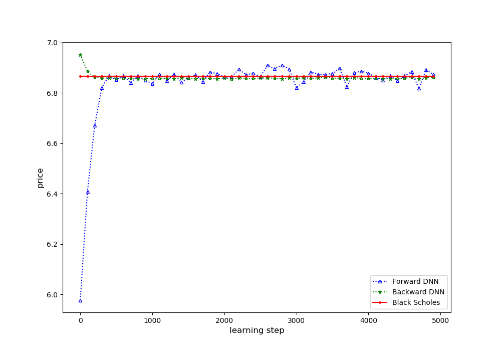
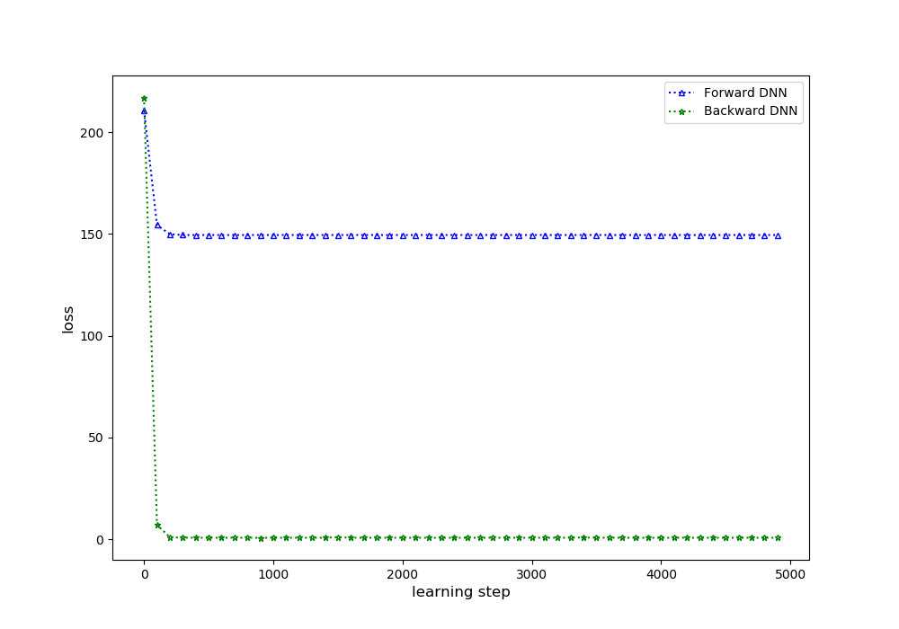
Figure 5.1: Comparison between forward and backward DNN on European call option

5.2 Tests on Bermudan options

In this section, we use 1Y ATM Bermudan options to test the performance of our least square backward DNN method. We test Bermudan call options on a single underlying stock, 2 underlying stocks (stock 1, 2), 3 underlying stocks (stock 1, 2, 3) and 5 underlying stocks (stock 1, 2, 3, 4, 5). The strike is chosen as $\sum_{d}\omega_{i}X_{0}^{i}$ with equal weight $\omega_{i}=1/d$ so that the option is ATM. The Bermuda option can be exercised quarterly, or at $t=0.25,0.5,0.75,1.0$. We compare the prices from PDE and Monte Carlo with the prices from the least square backward DNN method. The results are presented in Table 5.3 and Figure 5.2 - 5.5. It can be seen that the backward DNN method converges very fast and the convergence rate is not sensitive to the dimensions of the problem. The results for 10, 20 and 50 dimensions are presented in Section 5.4.2 and the largest difference between LSQ MC and the least square backward DNN method occurs at 50 dimensions with a difference of 0.4% (or 2.7 cents). Overall, the least square backward DNN method can produce very accurate prices for Bermudan call options.

Table 5.3: Comparison among PDE, Monte Carlo and least square backward DNN method on Bermudan options

1Y ATM Bermudan Call	PDE	LSQ MC	LSQ BDNN	rel diff from PDE	rel diff from LSQ MC
single stock (stock 1)	6.9933	6.9923	6.9863	-0.10%	-0.09%
2 stocks (stock 1, 2)	9.9514	9.9535	9.9488	-0.03%	-0.05%
3 stocks (stock 1, 2, 3)	9.6987	9.7224	9.6813	-0.18%	-0.42%
5 stocks (stock 1, 2, 3, 4, 5)		8.2709	8.2795		0.10%

Figure 5.2: Bermudan Call, single underlying stock

Figure 5.3: Bermudan Call, 2 underlying stocks

Figure 5.4: Bermudan Call, 3 underlying stocks

Figure 5.5: Bermudan Call, 5 underlying stocks

5.3 Tests on callable yield notes

In this section, we use 1Y CYNs to test the performance of our least square backward DNN method for complex payoffs. We test CYNs on a single underlying stock, 2 underlying stocks (stock 1, 2), 3 underlying stocks (stock 1, 2, 3) and 5 underlying stocks (stock 1, 2, 3, 4, 5). Some key contract parameters of the tested CYNs are provided in Table 5.4. We compare the prices from PDE and Monte Carlo with the prices from the least square backward DNN method. The results are presented in Table 5.5 and Figure 5.6 - 5.9. It can be seen that all the tested samples converge fast and the differences in prices between the backward DNN approach and PDE or MC method is very small. The results for 10, 20 and 50 dimensions are presented in Section 5.4.2. Overall, very accurate prices can be obtained with the least square backward DNN. Similar to Bermudan options, the largest difference between LSQ MC and the least square backward DNN method occurs at 50 dimensions with a difference of 1.5% (or 1.5 cents). The results indicates the validity and accuracy of the least square backward DNN method even when the payoff is complex.

Table 5.4: CYN contract parameters

contingent coupon	$r_{i}=5\%$
coupon barrier	$B_{i}=70\%$
knock-in barrier	$B=50\%$
knock-in put strike	$K=100\%$
call/coupon schedule	quarterly or 0.25, 0.5, 0.75, 1.0

Table 5.5: Comparison among PDE, Monte Carlo and least square backward DNN method on CYNs

1Y CYN	PDE	LSQ MC	LSQ BDNN	rel diff from PDE	rel diff from LSQMC
single stock (stock 1)	1.0475	1.0474	1.0474	-0.01%	0.00%
2 stocks (stock 1, 2)	1.0457	1.0458	1.0465	0.08%	0.07%
3 stocks (stock 1, 2, 3)	1.0438	1.0453	1.0452	0.13%	-0.02%
5 stocks (stock 1, 2, 3, 4, 5)		1.0449	1.0448		0.00%

Figure 5.6: CYN, single underlying stock

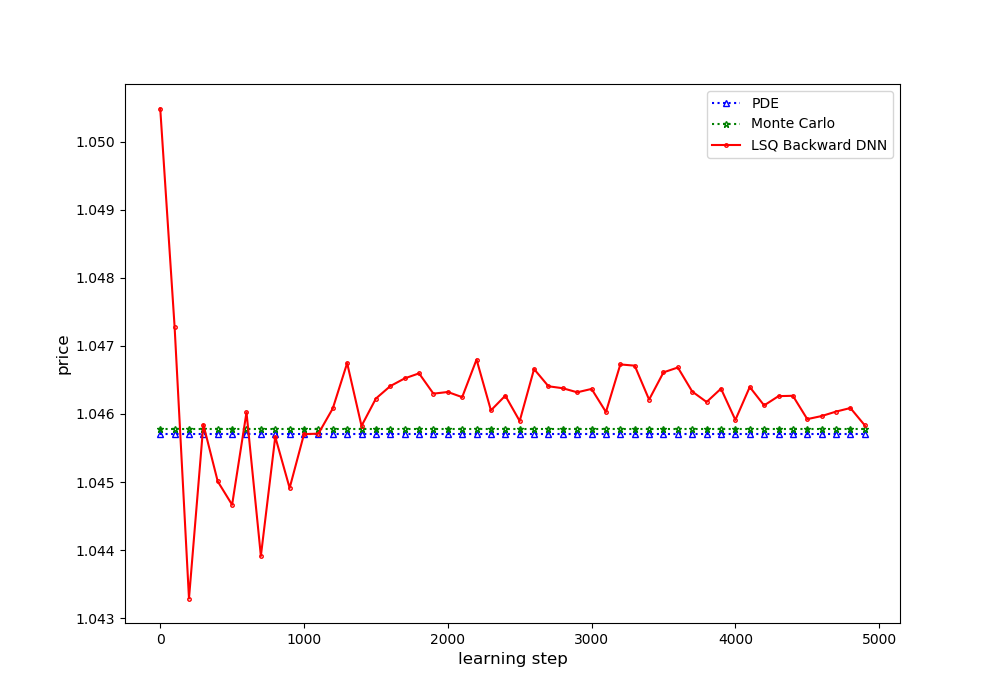
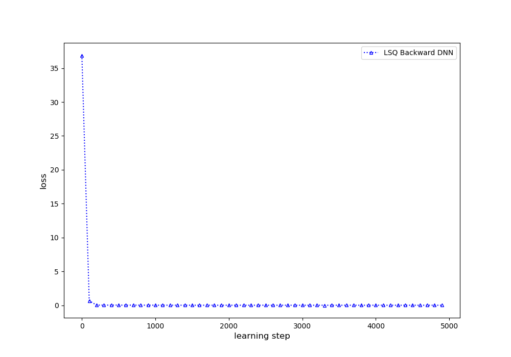
Figure 5.7: CYN, 2 underlying stocks

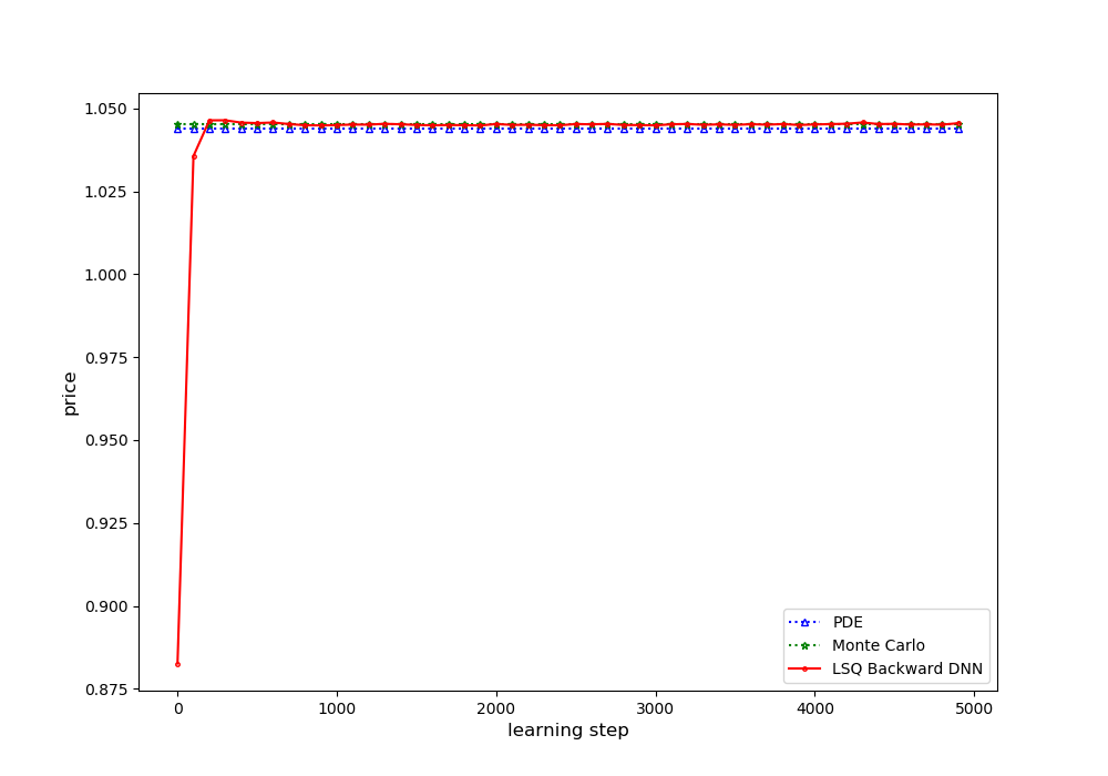
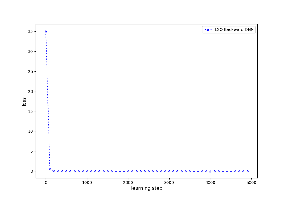
Figure 5.8: CYN, 3 underlying stocks

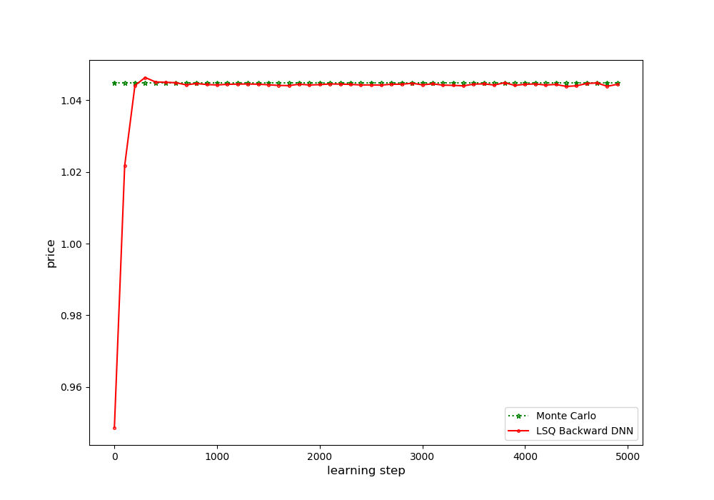
Figure 5.9: CYN, 5 underlying stocks

5.4 Efficiency test

In this section, we use a 1Y European option, a 1Y Bermudan option and a 1Y CYN to compare the computation efficiency between the DNN method and classical Monte Carlo method (least square Monte Carlo for Bermudan options and CYNs). We select 5 underlying stocks (stock 1, 2, …, 5), 10 underlying stocks (stock 1, 2, …, 10), 20 underlying stocks (repeat the 10 stocks twice) and 50 underlying stocks (repeat the 10 stocks five times) in our tests. The European/Bermudan option contract characteristics are analogous to those in Section 5.2. The strike is chosen as $\sum_{d}\omega_{i}X_{0}^{i}$ with equal weight $\omega_{i}=1/d$ so that the option is ATM. The Bermuda option can be exercised quarterly, or at $t=0.25,0.5,0.75,1.0$. The CYN contract characteristics are analogous to those in Section 5.3. The same parameters are used. For the classical MC (either the regular classical MC or the least square MC) we use $M=1,000,000$ sampling paths to estimate the means. For the least square backward DNN solver, the MC sampling size is 5,000 and 500 optimization iterations of training and validate the trained DNN every 10 iterations. This produces 50 results. We use the mean(standard error) of the 10 results with the least loss function value as our derivative price(standard error).

We performed our tests on both a desktop and a server. The testing desktop has CPU (Intel(R) Xeon(R) Silver 4108 @1.80GHz) with 8 cores/16 threads and 24GB RAM. The sever has 72 cores and 768GB RAM and each core is Intel(R) Xeon(R) E5-2699 v3 @2.30GHz.

It is well known that the parallelization of the least square Monte Carlo, widely used in high-dimensional American/Bermudan option pricing in practice, is a challenging task as the regression consumes most of the computation time for American options and Bermuda options with many early exercise times. However, since regression at each exercise date requires the cross-sectional information from all paths, regression step is not straightforward to parallelize. Realizing this characteristics, [4] parallelized the singular value decomposition in the regression step. Together with path generation parallelized, an efficient ratio (speed up factor/number of processors) of 56% is achieved on a IBM Blue Gene. [3] proposed to apply space decomposition to both the path generation phase and the regression/valuation phases. In Chen et al.’s work each sub-sample is an independent least square MC run. The authors found that the speed-up efficiency can be around 100% for 8 processes and around 80% for 64 processes. Even though there is significant improvement in parallelization efficiency, pricing bias is observed and the magnitude of the bias increases with the increase in the number of processes. Therefore, instead of using sub-sampling as the parallelization strategy, we used the least square regression routine in TensorFlow to implement the regression step in the classical least-square MC after the MC samples are generated. This choice is in the same spirit as the approach from Choudhury et al., i.e. parallelizing the most time consuming component of the process. Since the classical least-square MC is our benchmark to assess the accuracy of our backward DNN method, our approach avoids potential sub-sampling bias in the results from classical least-square MC. In addition, since the computational resources are fully managed by TensorFlow for both classical least-square MC and backward DNN, we have a fair comparison of efficiency for the two approaches.

5.4.1 Efficiency tests on European options

The testing results for a European option from 5 dimensions to 50 dimensions are presented in Table 5.6. It can seen that backward DNN method can produce prices very close (around 2 cents or less) to those from classical MC. Though classical MC is faster, it can not produce results for 20 dimensions and above with a desktop due to memory issues. The backward DNN method is slower, but results can be produced with all the cases we tested since it does not need a large number of samples to produce accurate results. Apparently, in general, if one has sufficient computational resource, DNN method is not efficient to price European style options as it is 5 to 6 times slower than the classical MC, primarily caused by the high cost in the DNN initialization and optimization. However, if one only has a machine with limited memory, the DNN approach is a choice for large scale problems.

Table 5.6: Comparison between Monte Carlo and backward DNN method on European options

1Y ATM European Call	MC				BDNN
	price	std error	desktop(s)	server(s)	price	std error	desktop(s)	server(s)
5 stocks	8.1033	0.0142	78	57	8.1146	0.0169	486	330
10 stocks	7.2546	0.0127	157	112	7.2318	0.0159	882	544
20 stocks	6.8038	0.0119	-	230	6.7856	0.0144	1904	981
50 stocks	6.5121	0.0113	-	576	6.4975	0.0137	6290	2650

5.4.2 Efficiency tests on Bermudan options and CYNs

The testing results from 5 dimensions to 50 dimensions are presented in Table 5.7 for Bermudan options and in Table 5.8 for CYNs. First it can be seen that the backward DNN method (here the least square backward DNN) can produce prices very close (round 1 cent or less in most cases) to those from classical least square MC, an evidence of its validity and accuracy. It is also very interesting of note that for Bermudan options, the standard deviations of the results from backward DNN are very similar to the MC errors of the mean from classical MC approach with our choice of parameters. For CYNs, though the standard deviations of the results from backward DNN are one order of higher than the MC errors of the mean from classical MC approach, they are still sufficiently small. Similar to the efficient tests for European options, the classical MC approach, though 5 or more times faster,could not produce results for 20 dimensions and above with a desktop computer due to memory issues.

Table 5.7: Comparison between Monte Carlo and least square backward DNN method on Bermundan options

1Y ATM Bermudan Call	LSQ MC				LSQ BDNN
	price	std error	desktop(s)	server(s)	price	std error	desktop(s)	server(s)
5 stocks	8.2709	0.0124	82	60	8.2795	0.0160	509	345
10 stocks	7.4112	0.0110	177	116	7.4127	0.0153	972	569
20 stocks	6.9760	0.0103	-	237	6.9745	0.0141	2549	976
50 stocks	6.7372	0.0100	-	658	6.7100	0.0137	21552	3476

Table 5.8: Comparison between Monte Carlo and least square backward DNN method on CYNs

1Y CYN	LSQ MC				LSQ BDNN
	price	std error	desktop(s)	server(s)	price	std error	desktop(s)	server(s)
5 stocks	1.0449	0.0000	84	60	1.0448	0.0008	506	342
10 stocks	1.0402	0.0001	179	122	1.0390	0.0011	947	563
20 stocks	1.0257	0.0001	-	235	1.0236	0.0016	2860	1012
50 stocks	0.9778	0.0002	-	659	0.9633	0.0023	20947	3274

6 Conclusion

In this work, we have developed a deep learning-based least square forward-backward stochastic differential equation solver, which can be used in high-dimensional derivatives pricing. Our deep learning implementation follows a similar approach to the ones explored by [6, 8] and [20]. However, the forward DNN method is more suitable for European style derivative pricing and the backward DNN method from Wang et al. may not adequately account for early exercise features. In our approach, we embed the least square regression technique similar to that in the least square Monte Carlo method ([13]) to the backward DNN algorithm. Numerical testing results on Bermudan options and callable yield notes indicate that our least square backward DNN method can produce very accurate results based on comparisons with the finite difference based PDE approach and the classical Monte Carlo simulation. This method can be used in various derivative pricing applications such as Barrier option, American option, convertible bonds, etc. In conclusion, our least square backward DNN algorithm can serve as a generic numerical solver for pricing derivatives, and it is most suitable for high-dimensional derivatives with early exercises features. Though it is slower than the classical Monte Carlo, the backward DNN approach is very memory efficient and can handle large scale problems with less computational resources.

References

- [1] Barraquand, J., and Martineau, D. (1995). Numerical valuation of high dimensional multivariate american securities. The Journal of Financial and Quantitative Analysis 30(3), 383–405.
- [2] Broadie, M., and Glasserman, P. (2004). A stochastic mesh method for pricing high-dimensional american options. Journal of Computational Finance 7(4), 35–72.
- [3] Chen, C., Huang, K., and Lyuu, Y. (2015). Accelerating the least-square monte carlo method with parallel computing. The Journal of Supercomputing 71(9), 3593–3608.
- [4] Choudhury, A.R., King, A., Kumar, S., and Sabharwal, Y. (2008). Optimizations in financial engineering: The least-squares monte carlo method of longstaff and schwartz. In 2008 IEEE International Symposium on Parallel and Distributed Processing 1–11.
- [5] De Spiegeleer, J., Madan, D.B., Reyners, S., and Schoutens, W. (2018). Machine Learning for quantitative finance: fast derivative pricing, hedging and fitting. Quantitative Finance 18(10), 1635–1643.
- [6] E, W., Han, J., and Jentzen, A. (2017). Deep learning-based numerical methods for high-dimensional parabolic partial differential equations and backward stochastic differential equations. Communications in Mathematics and Statistics 5(4), 349–380.
- [7] Fujii, M., Takahashi, A., and Takahashi, M. (2019). Asymptotic expansion as prior knowledge in deep learning method for high dimensional BSDEs. Asia-Pacific Financial Markets 26(3), 391–408.
- [8] Han, J., Jentzen, A., and E, W. (2018). Solving high-dimensional partial differential equations using deep learning. Proceedings of the National Academy of Sciences 115(34), 8505–8510.
- [9] Hutchinson, J.M., Lo, A.W., and Poggio, T. (1994). A nonparametric approach to pricing and hedging derivative securities via learning networks. The Journal of Finance 49(3), 851–889.
- [10] Kohler, M., Krzyżak, A., and Todorovic, N. (2010). Pricing of high-dimensional american options by neural networks. Mathematical Finance 20(3), 383–410.
- [11] Hull, J.C., Chapter 1 Introduction. Options, Futures, and Other Derivatives, Pearson, 10th edition, 2018.
- [12] Kim, J., Kim, T., Jo, J., Choi, Y., Lee, S., Hwang, H., Yoo, M. and Jeong, D., A practical finite difference method for the three-dimensional Black–Scholes equation. European Journal of Operational Research, 2016, 252(1), 183–190.
- [13] Longstaff, F., and Schwartz, E. (2015). Valuing American options by simulation: a simple least-squares approach. The Review of Financial Studies 14(1), 113–147.
- [14] Mil’shtejn, G. (1975). Approximate integration of stochastic differential equations. Theory of Probability & Its Applications 19(3), 557–562.
- [15] Moreno, M., and Navas, J.F., On the Robustness of Least-Squares Monte Carlo (LSM) for Pricing American Derivatives. Review of Derivatives Research, 2003, 6, 107–128.
- [16] Raissi, M. (2018). Forward-backward stochastic neural networks: Deep learning of high-dimensional partial differential equations. arXiv:1804.07010.
- [17] Sirignano, J., and Spiliopoulos, K. (2017). Stochastic gradient descent in continuous time. SIAM Journal on Financial Mathematics 8(1), 933–961.
- [18] Sirignano, J., and Spiliopoulos, K. (2018). DGM: A deep learning algorithm for solving partial differential equations. Journal of Computational Physics 375(15), 1339–1364.
- [19] Stentoft, L., Assessing the least squares Monte-Carlo approach to American option valuation. Review of Derivatives Research, 2004, 7(2), 129–168.
- [20] Wang, H., Chen, H., Sudjianto, A., Liu, R., and Shen, Q. (2018). Deep learning-based BSDE solver for Libor market model with applications to Bermudan swaption pricing and hedging. arXiv:1807.06622.