MadMiner: Machine learning–based inference for particle physics

Abstract

Precision measurements at the LHC often require analyzing high-dimensional event data for subtle kinematic signatures, which is challenging for established analysis methods. Recently, a powerful family of multivariate inference techniques that leverage both matrix element information and machine learning has been developed. This approach neither requires the reduction of high-dimensional data to summary statistics nor any simplifications to the underlying physics or detector response. In this paper we introduce MadMiner, a Python module that streamlines the steps involved in this procedure. Wrapping around MadGraph5_aMC and Pythia 8, it supports almost any physics process and model. To aid phenomenological studies, the tool also wraps around Delphes 3, though it is extendable to a full Geant4-based detector simulation. We demonstrate the use of MadMiner in an example analysis of dimension-six operators in $ttH$ production, finding that the new techniques substantially increase the sensitivity to new physics.

I Introduction

Precision measurements at the Large Hadron Collider (LHC) experiments search for direct and indirect signals of physics beyond the Standard Model. Statistically, this requires constraining a typically high-dimensional parameter space, for instance the Wilson coefficients in an effective field theory (EFT) or the couplings and masses in a supersymmetric model. The data going into these analyses consists of a large number of observables, many of which can carry information on the parameters of interest.

The relation between model parameters and observables is typically best described by a suite of computer simulation tools for the hard interaction, parton shower, hadronization, and detector response. These tools take as input assumed parameters of the physics model, for instance a particular value for the Wilson coefficients of an EFT, and use Monte-Carlo methods to sample hypothetical observations. Unfortunately, they do not directly let us solve the inverse problem: given a set of observed events, it is not possible to explicitly calculate the likelihood of such a measurement as a function of the theory parameters. This intractability of the likelihood function is a major challenge for particle physics measurements.

Particle physicists have developed a range of techniques for this problem of likelihood-free inference. These can be roughly grouped into three categories Brehmer:2019bvj :

1. Traditionally, analyses are restricted to a small number of hand-picked observables. The likelihood function for these low-dimensional summary statistics can then be estimated with explicit parametric functions, histograms, kernel density estimation techniques, or Gaussian Processes Cranmer:2000du ; Cranmer:2012sba ; Frate:2017mai . Relatedly, Approximate Bayesian Computation rubin1984 ; beaumont2002approximate ; Alsing:2018eau ; Charnock:2018ogm is a family of Bayesian techniques that allow sampling from an approximate version of the posterior in the space of the summary statistics. Coming up with the newest and greatest kinematic observables is a popular pastime among phenomenologists. But limiting the analysis to a few summary statistics discards the information in all other directions in phase space. Even well-motivated variables often do not come close to the power of an analysis of the fully differential cross section Brehmer:2016nyr ; Brehmer:2017lrt .

2. Another approach aims to estimate the likelihood function of high-dimensional observables by approximating the effect of shower, hadronization, and detector response with simple transfer functions (or neglecting them altogether). In this approximation, the likelihood becomes tractable. This category includes the Matrix Element Method Kondo:1988yd ; Abazov:2004cs ; Artoisenet:2008zz ; Gao:2010qx ; Alwall:2010cq ; Bolognesi:2012mm ; Avery:2012um ; Andersen:2012kn ; Campbell:2013hz ; Artoisenet:2013vfa ; Gainer:2013iya ; Schouten:2014yza ; Martini:2015fsa ; Gritsan:2016hjl ; Martini:2017ydu ; Kraus:2019qoq , Optimal Observables Atwood:1991ka ; Davier:1992nw ; Diehl:1993br , and Shower and Event Deconstruction Soper:2011cr ; Soper:2012pb ; Soper:2014rya ; Englert:2015dlp . These methods make maximal use of the knowledge about the physics underlying the simulations. While these methods do not require picking summary statistics, the approximation of the detector response can lead to suboptimal results, the treatment of additional jet radiation is a challenge, and the evaluation of each event requires the calculation of a numerically expensive integral.

3. Over the last years methods based on machine learning have become increasingly popular. The industry standard in particle physics is to train a classifier (often a boosted decision tree or neural network) to classify events as coming from different sources (e. g. signal vs. background). Its output is used to define acceptance regions, accepted events are then usually analyzed with a traditional histogram-based measurement strategy. While this strategy is great at suppressing background events, it does not necessarily lead to the most precise parameter measurements when kinematic distributions change over the parameter space Brehmer:2016nyr .

   Only recently has there been an increased interest in using machine learning to estimate the likelihood, likelihood ratio, or (in a Bayesian setting) the posterior 2012arXiv1212.1479F ; 2014arXiv1410.8516D ; 2015arXiv150203509G ; Cranmer:2015bka ; Cranmer:2016lzt ; Louppe:2016aov ; 2016arXiv160508803D ; 2016arXiv160506376P ; 2016arXiv161110242D ; 2016arXiv160502226U ; gutmann2017likelihood ; 2017arXiv170208896T ; 2017arXiv170707113L ; 2017arXiv170507057P ; 2017arXiv171101861L ; 2018arXiv180400779H ; 2018arXiv180507226P ; 2018arXiv180509294L ; DBLP:journals/corr/abs-1806-07366 ; 2018arXiv180703039K ; 2018arXiv181001367G ; 2018arXiv181009899D ; Hermans:2019ioj ; Alsing:2019xrx ; 2019arXiv190507488G . These approaches have in common that they only require access to samples generated for different model parameter values. They can handle high-dimensional observables and do not require a choice of summary statistics. They also work natively with the output of the simulator, so they do not require any simplifications to the underlying physics or detector response. The estimate of the likelihood provided by these algorithms typically becomes exact in the limit of infinite training samples (assuming sufficient capacity and efficient training), but often a large number of simulations is required before a good performance is reached.

A new machine-learning-based approach that directly leverages matrix element information has been introduced in Refs. Brehmer:2018hga ; Brehmer:2018kdj ; Brehmer:2018eca and since been further developed in Refs. Stoye:2018ovl ; Brehmer:2019bvj . Like the other multivariate approaches, these techniques support high-dimensional observables without the restriction to summary statistics. Similar to the Matrix Element Method and Optimal Observables, these techniques leverage our physics insight in the form of the matrix elements efficiently. But unlike those methods, they support state-of-the-art simulations of the parton shower and detector response. In addition, after an upfront simulation and training phase, they provide a function that estimates the likelihood and can be evaluated in microseconds.

These new techniques require extracting matrix-element information from the Monte-Carlo simulation, keeping track of and manipulating these weights in specific ways, and then training machine learning models on this data. Without proper software support, these steps are cumbersome and error-prone, providing a technological hurdle to a wider adaptation of these methods. Reference Brehmer:2018hga describes this approach with the analogy of “mining gold” from Monte-Carlo simulations: while the additional information from the simulations is very valuable, it can require some effort to extract and process. But the gold does not have to be hard to mine!

In this paper we introduce MadMiner, a Python module that automates all steps necessary for these modern multivariate inference techniques. It supports all elements of a typical analysis, including the simulation of events with MadGraph5_aMC Alwall:2014hca , Pythia 8 Sjostrand:2007gs , detector simulation, reducible and irreducible backgrounds, and systematic uncertainties. For phenomenological studies, the tool supports the simulation of the detector response with Delphes 3 deFavereau:2013fsa , though it is extendable to a full detector simulation based on Geant4 Agostinelli:2002hh .

We review the supported analysis techniques in Sec. II and describe their implementation in MadMiner in Sec. III. In Sec. IV, the new tool is demonstrated in an example analysis of Higgs production in association with a top pair at the high luminosity run of the LHC. We give our conclusions in Sec. V. In the appendix we answer frequently asked questions.

II Inference techniques

II.1 LHC measurements as a likelihood-free inference problem

The ultimate goals of most measurements are best-fit points and exclusion regions in a (high-dimensional) parameter space. In particle physics experiments, best-fit points are typically defined as maximum likelihood estimators, while exclusion regions are based on hypothesis tests that use the (profile) likelihood ratio as test statistic Cranmer:2015nia . Both are based on the same central object, the likelihood function $p_{\text{full}}(\{x\}|\theta)$. It quantifies the probability of observing a set of events, where each event is characterized by a vector $x$ of observables such as reconstructed energies, momenta, and angles of all final-state particles, as a function of a vector of model parameters $\theta$, e. g. the Wilson coefficients of an effective field theory.

In particle physics measurements, the likelihood function usually has the form

$$p_{\text{full}}(\{x\}|\theta)=\operatorname{Pois}(n|L\sigma(\theta))\;\prod_{i}p(x_{i}|\theta)\,.$$ (1)

Here $n$ is the observed number of events, $L$ is the integrated luminosity, $\sigma(\theta)$ is the cross section as a function of the model parameters, $\operatorname{Pois}(n|\lambda)=\lambda^{n}e^{-\lambda}/n!$ is the probability mass function of the Poisson distribution, and

$$p(x|\theta)=\frac{1}{\sigma(x)}\frac{\mathrm{d}^{d}\sigma(x|\theta)}{\mathrm{d}x^{d}}$$ (2)

is the likelihood function for a single event: the probability density of the $d$-dimensional vector of observables $x$ as a function of the model parameters $\theta$. Up to the normalization, this kinematic likelihood function is identical to the fully differential cross section $\mathrm{d}^{d}\sigma(x|\theta)/\mathrm{d}x^{d}$.

The Poisson or rate term in Eq. (1) is comparably simple, even though it is based on the cross section after efficiency and acceptance effects, which can be complicated to calculate in realistic problems. But the remaining terms, which quantify the kinematic information, typically cannot be explicitly computed at all. This is because the most accurate model of the kinematic distributions is usually given by a complicated chain of Monte-Carlo simulators. The kinematic likelihood they implicitly define can be written symbolically as

$$p(x|\theta)=\int\!\mathrm{d}z_{d}\;\int\!\mathrm{d}z_{s}\;\int\!\mathrm{d}z_{p}\;\underbrace{p(x|z_{d})\,p(z_{d}|z_{s})\,p(z_{s}|z_{p})\,p(z_{p}|\theta)}_{p(x,z|\theta)}\,,$$ (3)

where $z_{p}$ are the four-momenta, charges, and helicities of the parton-level four-momenta, $z_{s}$ is the entire history of the parton shower, and $z_{d}$ describe the interactions of the particles with the detector. A state-of-the-art simulation can easily involve billions of such latent variables. Explicitly calculating the integral over this huge space is clearly impossible: given a set of events $\{x\}$ and a parameter point $\theta$, we hence cannot compute the likelihood function (it is intractable). This is a major challenge for analyzing LHC data. The same structural problem appears in many other fields that use computer simulations to model complicated processes, including cosmology, systems biology, and epidemiology, giving rise to the development of different likelihood-free inference techniques.

In particle physics, common analysis techniques address the intractability of the likelihood function in different ways. The traditional approach restricts the observables $x$ to one or two summary statistics $v(x)$, for instance the invariant mass of the decay products of a searched resonance or the transverse momentum of the hardest particle in an EFT analysis. Then the density $p(v|\theta)$ can be calculated with histograms and used in lieu of the full likelihood $p(x|\theta)$. On the other hand, the Matrix Element Method and Optimal Observable approaches simplify the integral in Eq. (3) by replacing the shower and detector response with simple smearing or transfer functions; in this approximation it also becomes tractable. For a discussion and comparison of these different methods see Ref. Brehmer:2019bvj .

II.2 Learning the likelihood function

A first class of inference techniques in MadMiner tackles the intractability of the likelihood function head-on: a neural network is trained to estimate the kinematic likelihood $p(x|\theta)$ or, equivalently, the likelihood ratio

$$r(x|\theta_{0},\theta_{1})=\frac{p(x|\theta_{0})}{p(x|\theta_{1})}$$ (4)

using data available from the simulator. To be more specific, MadMiner differentiates between three different functions that the neural network can learn:

Likelihood estimators

In this case, a neural network takes as input event data $x$ as well as a model parameter point $\theta$ and returns the estimated likelihood $\hat{p}(x|\theta)$,

$$\operatorname{NN}:(x,\theta)\mapsto\hat{p}(x|\theta)\,.$$ (5)

Likelihood ratio estimators

Alternatively, the network can model the likelihood ratio including its dependence on the data $x$ and on the parameter point $\theta$ in the numerator of the ratio,

$$\operatorname{NN}:(x,\theta)\mapsto\hat{r}(x|\theta)\approx\frac{p(x|\theta)}{p_{\text{ref}}(x)}\,.$$ (6)

There are different options for the denominator distribution $p_{\text{ref}}(x)$. In MadMiner we set it to the distribution from a reference parameter point, $p_{\text{ref}}(x)=p(x|\theta_{\text{ref}})$. Alternatively, it could be given by a marginal model $p_{\text{ref}}(x)=\int\!\mathrm{d}\theta^{\prime}\;p(x|\theta^{\prime})p(\theta^{\prime})$, or even be an entirely unphysical reference distribution.

Doubly parameterized likelihood ratio estimators

The last option is to model the likelihood ratio as a function of not only the event data $x$ and the numerator parameter point $\theta_{0}$, but also including its dependence on the denominator model,

$$\operatorname{NN}:(x,\theta_{0},\theta_{1})\mapsto\hat{r}(x|\theta_{0},\theta_{1})\approx\frac{p(x|\theta_{0})}{p(x|\theta_{1})}\,.$$ (7)

Note that in all three cases, the network is parameterized in terms of the theory parameters $\theta$ Cranmer:2015bka ; Baldi:2016fzo : rather than training separate networks for different points on a grid of parameter points, one neural network models the likelihood function for the whole parameter space. The network learns to interpolate in parameter space and can “borrow” statistical power from close parameter points, leading to a significantly better sample efficiency than a point-by-point approach Brehmer:2018eca .

Method	Run simulation at	Loss fn. uses		Asympt. exact	Generative	Ref.
		$r(x,z)$	$t(x,z)$
Likelihood estimators
NDE	$\theta\sim\pi(\theta)$			$\checkmark$	$\checkmark$	2017arXiv170507057P
Scandal	$\theta\sim\pi(\theta)$		$\checkmark$	$\checkmark$	$\checkmark$	Brehmer:2018hga
Likelihood ratio estimators
Carl	$\theta\sim\pi(\theta)$, $\theta_{\text{ref}}$			$\checkmark$		Cranmer:2015bka
Rolr	$\theta\sim\pi(\theta)$, $\theta_{\text{ref}}$	$\checkmark$		$\checkmark$		Brehmer:2018eca
Alice	$\theta\sim\pi(\theta)$, $\theta_{\text{ref}}$	$\checkmark$		$\checkmark$		Stoye:2018ovl
Cascal	$\theta\sim\pi(\theta)$, $\theta_{\text{ref}}$		$\checkmark$	$\checkmark$		Brehmer:2018eca
Rascal	$\theta\sim\pi(\theta)$, $\theta_{\text{ref}}$	$\checkmark$	$\checkmark$	$\checkmark$		Brehmer:2018eca
Alices	$\theta\sim\pi(\theta)$, $\theta_{\text{ref}}$	$\checkmark$	$\checkmark$	$\checkmark$		Stoye:2018ovl
Doubly parameterized likelihood ratio estimators
Carl	$\theta_{0}\sim\pi(\theta)$, $\theta_{1}\sim\pi(\theta)$			$\checkmark$		Cranmer:2015bka
Rolr	$\theta_{0}\sim\pi(\theta)$, $\theta_{1}\sim\pi(\theta)$	$\checkmark$		$\checkmark$		Brehmer:2018eca
Alice	$\theta_{0}\sim\pi(\theta)$, $\theta_{1}\sim\pi(\theta)$	$\checkmark$		$\checkmark$		Stoye:2018ovl
Cascal	$\theta_{0}\sim\pi(\theta)$, $\theta_{1}\sim\pi(\theta)$		$\checkmark$	$\checkmark$		Brehmer:2018eca
Rascal	$\theta_{0}\sim\pi(\theta)$, $\theta_{1}\sim\pi(\theta)$	$\checkmark$	$\checkmark$	$\checkmark$		Brehmer:2018eca
Alices	$\theta_{0}\sim\pi(\theta)$, $\theta_{1}\sim\pi(\theta)$	$\checkmark$	$\checkmark$	$\checkmark$		Stoye:2018ovl
Score estimators
Sally	$\theta_{\text{ref}}$		$\checkmark$	in local approx.		Brehmer:2018eca
Sallino	$\theta_{\text{ref}}$		$\checkmark$	in local approx.		Brehmer:2018eca

Table 1: Inference techniques implemented in MadMiner. We separate them into four groups, depending on which quantity is estimated by the neural network; see the text for more details. We give the parameter values for which the Monte-Carlo samples have to be generated and list whether the augmented data (joint likelihood ratio $r(x,z)$ and joint score $t(x,z)$) are used. “Asymptotically exact” describes methods that should give theoretically optimal results in the limit of sufficient network capacity, perfect optimization, and enough training data. Methods that also allow for the fast generation of event data from the neural network are marked as “generative”. Finally, for each method we provide the reference that provides the clearest explanation (and spells out the acronym).

But how do we train a neural network to learn any of these three functions? More specifically, which loss function can we minimize so that a neural network will converge to the right function? There are a number of different answers, which can be grouped into two categories. First, some methods have been developed that just use samples of events $\{x\}$ generated from different parameter points $\theta$. This includes neural density estimation (NDE) techniques, for instance masked autoregressive flows 2017arXiv170507057P , in which the network learns the likelihood function. Another approach is the Carl method Cranmer:2015bka , which trains the network to estimate the likelihood ratio.

While both NDE and Carl are implemented in MadMiner, its major feature is the support for a new, potentially more powerful paradigm to likelihood or likelihood ratio estimation Brehmer:2018hga ; Brehmer:2018kdj ; Brehmer:2018eca . The key idea is that additional information can be extracted from the Monte-Carlo simulations, and that this additional information can be used to train more precise estimators of likelihood or likelihood ratio with less training data.

More specifically, for each simulated event it is possible to calculate the joint likelihood ratio

$$r(x,z|\theta_{0},\theta_{1})\equiv\frac{p(x,z|\theta_{0})}{p(x,z|\theta_{1})}=\frac{p(x|z_{d})\,p(z_{d}|z_{s})\,p(z_{s}|z_{p})\,p(z_{p}|\theta_{0})}{p(x|z_{d})\,p(z_{d}|z_{s})\,p(z_{s}|z_{p})\,p(z_{p}|\theta_{1})}=\frac{\mathrm{d}\sigma(z_{p}|\theta_{0})}{\mathrm{d}\sigma(z_{p}|\theta_{1})}\,\frac{\sigma(\theta_{1})}{\sigma(\theta_{0})}$$ (8)

and the joint score

$$t(x,z|\theta)\equiv\nabla_{\theta}\log p(x,z|\theta)=\frac{p(x|z_{d})\,p(z_{d}|z_{s})\,p(z_{s}|z_{p})\,\nabla_{\theta}p(z_{p}|\theta)}{p(x|z_{d})\,p(z_{d}|z_{s})\,p(z_{s}|z_{p})\,p(z_{p}|\theta)}=\frac{\nabla_{\theta}\mathrm{d}\sigma(z_{p}|\theta)}{\mathrm{d}\sigma(z_{p}|\theta)}-\frac{\nabla_{\theta}\sigma(\theta)}{\sigma(\theta)}\,.$$ (9)

Here $\sigma(\theta)$ is the total cross section as a function of the model parameters $\theta$, and $\mathrm{d}\sigma(z_{p}|\theta)$ are the parton-level event weights. At a hadron collider such as the LHC these can be written as Alwall:2010cq

$$\mathrm{d}\sigma(z_{p}|\theta)=\frac{(2\pi)^{4}f_{1}(\mathrm{x}_{1},Q^{2})f_{2}(\mathrm{x}_{2},Q^{2})}{2\mathrm{x}_{1}\mathrm{x}_{2}s}\;|\mathcal{M}|^{2}(z_{p}|\theta)\;\mathrm{d}\Phi(z_{p})\,.$$ (10)

They depend on the momentum fractions $\mathrm{x}_{i}$ carried by the initial-state partons, the squared center-of-mass energy $s$, the momentum transfer $Q$, the corresponding values of the parton density functions $f_{i}(\mathrm{x}_{i},Q^{2})$, and the Lorentz-invariant phase-space element $\mathrm{d}\Phi(z_{p})$. Finally, $z_{p}$ is the entire phase-space point of a simulated event (including the parton four-momenta, helicities, and charges), and $|\mathcal{M}|^{2}(z_{p}|\theta)$ is the squared matrix element. Both the joint likelihood ratio and the joint score thus depend on the parton-level momenta $z_{p}$ and are directly related to the squared matrix element describing the underlying process.

The main insight of Refs. Brehmer:2018hga ; Brehmer:2018kdj ; Brehmer:2018eca is that the joint likelihood ratio and joint score can be used to define loss functions that, when minimized with respect to a test function that only depends on $x$ and $\theta$, converges to the likelihood function $p(x|\theta)$ or the likelihood ratio.

There are several variations of this idea. The main difference between them is the exact form of the loss function used. We label them with a set of acronyms: Scandal is an improved version of NDE techniques that uses the joint score to train likelihood estimators more efficiently; Cascal is a similarly improved version of the Carl method; Rolr and Alice use the joint likelihood ratio to efficiently train a likelihood ratio estimator; and finally the Rascal and Alices techniques use both the joint likelihood ratio and the joint score, maximizing the use of information from the simulator. In Tbl. 1 we provide an overview and give references to detailed explanations of all methods.

Once a neural network has been trained with one of these methods, it can calculate an estimated value of the likelihood or likelihood ratio for any event and any parameter point. Established statistical tools can then be used to calculate best-fit points and exclusion limits in the parameter space. For the calculation of frequentist confidence regions, there are generally two strategies. The first is simulating a large number of toy experiments to calculate the $p$-value for each parameter point that is tested. This approach can be computationally expensive, but guarantees statistically correct results — even if the neural network has not learned the likelihood function accurately, this approach will not lead to too tight limits. The second strategy uses the asymptotic properties of the likelihood ratio function Wilks:1938dza ; Wald ; Cowan:2010js to directly translate values of the likelihood ratio into $p$-values. While this method is extremely efficient, it relies on correctly trained neural networks.

II.3 Learning locally optimal observables

MadMiner also implements a second class of methods: rather than trying to reconstruct the full likelihood function, a neural network is trained to provide the most powerful observables for a given measurement problem. The central quantity of this approach is the score

$$t(x)=\nabla_{\theta}\log p(x|\theta)\biggr{|}_{\theta_{\text{ref}}}$$ (11)

evaluated at a fixed reference parameter point $\theta_{\text{ref}}$, for instance the SM. This vector has one component per parameter. For a given event $x$, its components are just numbers (unlike the likelihood and the likelihood ratio, which are also functions of the parameters $\theta$). In other words, the score is a vector of observables.

The relevance of these observables is most obvious in a local approximation of the likelihood function Alsing:2017var ; Brehmer:2018kdj ; Alsing:2018eau : in the neighborhood of the parameter point $\theta_{\text{ref}}$, the score components are the sufficient statistics. That means that for the purpose of measuring $\theta$, knowing $t(x)$ is just as powerful as knowing the full likelihood $p(x|\theta)$ (which, since it depends on $\theta$, is a much more complicated object). In this sense, the score defines the most powerful observables for the measurement of $\theta$.

This motivates a fourth function for a neural network to estimate:

Score estimator

A neural network takes as input event data $x$ and returns the estimated score at a reference parameter point,

$$\operatorname{NN}:x\mapsto\hat{t}(x)\approx\nabla_{\theta}\log p(x|\theta)\biggr{|}_{\theta_{\text{ref}}}$$ (12)

How does a neural network learn to estimate the score? Again, extracting additional information from the simulator proves useful. The Sally and Sallino methods introduced in Refs. Brehmer:2018hga ; Brehmer:2018kdj ; Brehmer:2018eca define a loss function that involves the joint score $t(x,z)$. Minimizing this loss function will train a neural network to converge to the true score $t(x)$ (Brehmer:2018hga, ).

After training, such a score estimator can be used like any other set of observables. In particular, we can fill multivariate histograms of the score and use them for inference. This approach, named Sally, requires only a minimal modification of established analysis workflows. A similar method called Sallino constructs one-dimensional histograms of particular projections of the estimated score, see Ref. Brehmer:2018eca for details.

As long as parameter points close to the reference point, for instance the SM, are analyzed, and assuming that the neural network was trained efficiently and with enough training data, the Sally or Sallino methods will lead to statistically optimal limits. Further away from the reference point, the score components might no longer be optimal, and this approach might lose some power compared to the techniques discussed in the previous section. The size of the parameter region in which the score components are the sufficient statistics depends on the size of higher derivatives of the (log) likelihood with respect to the parameters and is not known a priori; we will illustrate this with an example in Sec. IV.3.

II.4 The Fisher information

The final results of actual measurements are best-fit points and exclusion limits. However, for quickly evaluating the sensitivity of a measurement, comparing different channels, or optimizing an analysis, a different object is often more practical: the Fisher information matrix. It is closely connected to the score discussed in the previous section and summarizes the sensitivity of an analysis in a compact, interpretable, and powerful way Brehmer:2016nyr ; Brehmer:2017lrt . It is defined as the expectation value

$$I_{ij}(\theta)=\mathbb{E}\left[\frac{\partial\log p_{\text{full}}(\{x\}|\theta)}{\theta_{i}}\,\frac{\partial\log p_{\text{full}}(\{x\}|\theta)}{\theta_{j}}\middle|\theta\right]$$ (13)

with the full likelihood function $p_{\text{full}}(\{x\}|\theta)$ from Eq. (1).

To see why this matrix is useful, consider an expansion of the expected log likelihood ratio between $\theta+\Delta\theta$ and $\theta$ around the minimum:

$$-2\;\mathbb{E}\left[\log\frac{p_{\text{full}}(\{x\}|\theta+\Delta\theta)}{p_{\text{full}}(\{x\}|\theta)}\middle|\theta\right] =-\mathbb{E}\left[\frac{\partial^{2}\log p_{\text{full}}(\{x\}|\theta)}{\partial\theta_{i}\;\partial\theta_{j}}\middle|\theta\right]\;\Delta\theta_{i}\;\Delta\theta_{j}+\mathcal{O}(\Delta\theta^{3})$$

$$=\mathbb{E}\left[\frac{\partial\log p_{\text{full}}(\{x\}|\theta)}{\partial\theta_{i}}\;\frac{\partial\log p_{\text{full}}(\{x\}|\theta)}{\partial\theta_{j}}\middle|\theta\right]\;\Delta\theta_{i}\;\Delta\theta_{j}+\mathcal{O}(\Delta\theta^{3})$$

$$=I_{ij}(\theta)\;\Delta\theta_{i}\;\Delta\theta_{j}+\mathcal{O}(\Delta\theta^{3})$$

$$=d(\theta,\theta+\Delta\theta)^{2}+\mathcal{O}(\Delta\theta^{3})\,.$$ (14)

In the last step we have introduced the local Fisher distance

$$d(\theta+\Delta\theta,\theta)=\sqrt{I_{ij}(\theta)\;\Delta\theta_{i}\;\Delta\theta_{j}}$$ (15)

which is a convenient approximation of the log likelihood ratio as long as $\Delta\theta$ is small. Moreover, according to the Cramér-Rao bound Rao:1945 ; Cramer:1946 the inverse of the Fisher information is the minimal covariance of any estimator $\hat{\theta}$. The larger the Fisher information, the more precisely a parameter can be measured.

This approach shines when it comes to ease of use and interpretability. The Fisher information matrix is invariant under reparameterizations of the observables $x$, transforms covariantly under reparameterizations of the parameters $\theta$, and is additive over phase-space regions. This property means we can define the distribution of the differential information over phase space, which quantifies where in phase space the power of an analysis comes from Brehmer:2016nyr . The formalism also easily accommodates nuisance parameters, and profiling over them is a simple matrix operation Brehmer:2016nyr ; Edwards:2017mnf .

In particle physics processes described by Eq. (1), the Fisher information turns out to be Brehmer:2016nyr

$$I_{ij}(\theta) =\frac{L\,\partial_{i}\sigma(\theta)\,\partial_{j}\sigma(\theta)}{\sigma(\theta)}+L\,\sigma(\theta)\;\int\!\mathrm{d}x\;p(x|\theta)\,t_{i}(x|\theta)\,t_{j}(x|\theta)$$

$$\approx\frac{L\,\partial_{i}\sigma(\theta)\,\partial_{j}\sigma(\theta)}{\sigma(\theta)}+\frac{L\,\sigma(\theta)}{n}\;\sum_{x\sim p(x|\theta)}t_{i}(x|\theta)\,t_{j}(x|\theta)\,,$$ (16)

where $L$ is the integrated luminosity, $\sigma$ the cross section, $\partial_{i}$ denotes derivatives with respect to $\theta_{i}$, $n$ is the number of events $x$ generated for the parameter point $\theta$, and $t_{i}$ is the $i$-th component of the score vector introduced in Eq. (11). The first term describes the information in the overall rate, while the second term quantifies the power in the kinematic distributions. A neural score estimator $\hat{t}(x)$ as in Eq. (12) together with a set of events thus lets us calculate the (a priori intractable) Fisher information.

II.5 Practical analysis aspects

Let us now link these abstract inference techniques to specific aspects of typical analyses in high-energy physics and summarize some features and limitations of MadMiner.

High-energy process

MadMiner supports almost all processes of perturbative high-energy physics that can be run in MadGraph5_aMC Alwall:2014hca . This includes any high-energy physics model specified in the UFO format Degrande:2011ua . The inference techniques only require that the model is parameterized by a finite number of model parameters $\theta$ and that it is possible to calculate the parton-level event weights of Eq. (10) for arbitrary values of the model parameters $\theta$, i. e. to “reweight” the events to different parameter points Mattelaer:2016gcx . The approach is not fundamentally restricted to leading order, though one has to be careful that negative event weights, which can appear in certain subtraction schemes, do not lead to numerical instabilities.

It is often beneficial to define the parameters $\theta$ such that they span a similar order of magnitude. In practice, this may require some rescaling. For instance, if an analysis aims to measure two Wilson coefficients $f_{0}$ and $f_{1}$ and the range of interest of $f_{1}$ is 1000 times larger than that of $f_{0}$, consider defining the parameters internally as $\theta=(f_{0},f_{1}/1000)$.

Morphing

In an important class of models the squared matrix elements (or parton-level event weights) can be factorized into a sum over $n_{c}$ components, each consisting of an analytical function of the theory parameters times a function of phase-space:

$$|\mathcal{M}|^{2}(z_{p}|\theta)=\sum_{c}w_{c}(\theta)\,f_{c}(z_{p})\,.$$ (17)

This is often the case in effective field theories, or when indirect effects of new physics are parameterized through form factors.

For instance, consider the simple case in which we are trying to measure a single BSM parameter $\theta$ and the process is described by a SM contribution, an interference term, and a squared BSM amplitude:

$$|\mathcal{M}|^{2}(z_{p}|\theta)=\underbrace{1\vphantom{M_{M}^{\dagger}}}_{w_{0}(\theta)\vphantom{f_{0}}}\,\underbrace{|\mathcal{M}_{SM}|^{2}(z_{p})}_{f_{0}(z_{p})}+\underbrace{\theta\vphantom{M_{M}^{\dagger}}}_{w_{1}(\theta)\vphantom{f_{0}}}\,\underbrace{2\operatorname{Re}\mathcal{M}_{SM}^{\dagger}(z_{p})\,\mathcal{M}_{BSM}(z_{p})}_{f_{1}(z_{p})}+\underbrace{\theta^{2}\vphantom{M_{M}^{\dagger}}}_{w_{2}(\theta)\vphantom{f_{0}}}\,\underbrace{|\mathcal{M}_{BSM}|^{2}(z_{p})}_{f_{2}(z_{p})}\,.$$ (18)

More generally, the dependency on the model parameters is often a combination of different polynomials. Note that the contributions $f_{c}(z_{p})$ are not necessarily distributions: they can be negative, or integrate to zero, for instance for interference terms. Nevertheless, the sum of all components is always a physical distribution, i. e. it is non-negative everywhere and integrates to the total cross section.

When a process factorizes according to Eq. (17), a “morphing technique” ATLAS:morphing ; Brehmer:2018eca allows us to calculate event weights anywhere in parameter space precisely and very fast. First, the squared matrix element is evaluated at $n_{c}$ different points in the parameter space. The structure of Eq. (17) together with some linear algebra is then used to exactly interpolate to any other parameter point. This process is described in detail in Ref. Brehmer:2018eca .

MadMiner implements this morphing technique and leverages it extensively. The user only has to specify the maximal powers with which each model parameter contributes to the squared matrix element. MadMiner then automates the necessary linear algebra internally.

A practical question is at which $n_{c}$ benchmark points the matrix elements should be evaluated originally. This set of parameter points is called the morphing basis. While the physical predictions for a given parameter point are independent of this basis, the morphing procedure involves matrix inversions and cancellations between potentially large terms that depend on the choice of basis. Some morphing basis choices can thus lead to floating-point precision issues, while others are numerically more stable. MadMiner can automatically pick or complete a morphing basis that avoids or minimizes numerical precision issues. This optimization consists of randomly drawing a number of basis configurations over a user-specified parameter region, calculating morphing weights for each basis, and choosing the basis that minimizes the sum of squared morphing weights.

Note that MadMiner is not restricted to problems that factorize according to Eq. (17). Much of the core functionality is available for almost any model of new physics. But some features are currently only implemented in the morphing case, and for others the morphing setup can reduce the computational cost substantially.

Parton shower

Parton shower and hadronization can be simulated with Pythia 8 Sjostrand:2007gs , including matching and merging of different final-state jet multiplicities. This part of the event evolution should not directly depend on the new physics parameters of interest. Other shower simulators can be interfaced with little effort.

Detector simulation

Out of the box, MadMiner includes a fast phenomenological detector simulation with Delphes 3 deFavereau:2013fsa , as well as an alternative approximate detector simulation through smearing functions based on the parton-level final state. MadMiner is designed modularly so that it can be interfaced to more realistic detector simulations used by the experimental collaborations such as Geant4 Agostinelli:2002hh . Such an extension will mostly require careful book-keeping of event weights and observables.

Observables

The observed data for each event needs to be parameterized in a fixed-length vector of observables $x$. These can include both basic characteristics like energies, transverse momenta, and angular directions of reconstructed particles, but also higher-level features such as invariant masses or angular correlations between particles. For Delphes-level analyses, MadMiner allows the definition of these observables as arbitrary functions of the objects in the Delphes output file, while for parton-level analyses arbitrary functions of the smeared parton-level four-momenta are supported. It is possible to extend MadMiner with interfaces to any external code that calculates observables from generated events.

Backgrounds

Different signal and background processes, with no limitations on the parton-level final states, can be combined in the same analysis. Background processes are allowed to depend on the model parameters $\theta$. In the case of a reducible backgrounds that are not affected by $\theta$, the joint log likelihood ratio and joint score of all background events are zero, up to an $x$-independent constant that is related to the dependence of the overall signal cross section on $\theta$. We will discuss and illustrate this case in Sec. IV.1.

While fully data-driven backgrounds are not supported, a data-driven normalization of MC event samples is possible.

Systematic uncertainties

All imperfections in the description of the physics process with the simulation chain are modeled with nuisance parameters $\nu$. For most of the analysis chain, they play the same role as the physics parameters of interest $\theta$: their true value is unknown and they affect the likelihood of simulation outcomes. For the inference techniques presented in the previous section, every occurence of $\theta$ then has to be replaced with $(\theta,\nu)$: the neural networks estimate the likelihood $p(x|\theta,\nu)$, the likelihood ratio $r(x|\theta_{0},\nu_{0};\theta_{1},\nu_{1})$, or the score $t(x|\theta,\nu)$, where the latter now has more components corresponding to both the gradient with respect to $\theta$ and the gradient with respect to $\nu$. At the final limit setting stage, one then picks a constraint term (or, in a Bayesian setting, a prior) for the nuisance parameters and profiles (or marginalizes) over them, following established statistical procedures Cowan:2010js ; Brehmer:2016nyr ; Edwards:2017mnf ; Alsing:2019dvb .

MadMiner currently supports nuisance parameters that model systematic uncertainties from scale and PDF choices. The effect of the nuisance parameters on an event weight is parameterized as

$$\mathrm{d}\sigma(z_{p}|\theta,\nu)=\mathrm{d}\sigma(z_{p}|\theta,0)\times\exp\left[\sum_{i}\left(a(z_{p})\,\nu_{i}+b(z_{p})\,\nu_{i}^{2}\right)\right]\,,$$ (19)

similar to HistFactory Cranmer:2012sba and PyHF PYHF . $\nu_{i}=0$ corresponds to the nominal value of the $i$-th nuisance parameter. For each varied scale, $\nu_{i}=\pm 1$ correspond to the scale variations (typically half and twice the nominal scale choice). PDF uncertainties are described by one nuisance parameter per eigenvector in a Hessian PDF set, and $\nu_{i}=1$ corresponds to the event weight along a unit step of an eigenvector. The factors $a(z_{p})$ and $b(z_{p})$ are automatically calculated for each event based on a reweighting procedure Frederix:2011ss . The exponential form of Eq. (19) ensures non-negative event weights.

Neural network architectures and training

The heart of MadMiner’s analysis techniques are neural networks that take event data $x$ (and, depending on the method, a parameter point $(\theta,\nu)$) as input and return the likelihood, likelihood ratio, or score. The optimal architecture of these networks depends on the problem. MadMiner currently supports fully connected feed-forward neural networks with a variable number of layers and hidden units and different activation functions, implemented in PyTorch paszke2017automatic . The loss functions are mostly fixed by the inference methods given in Tbl. 1. The Scandal, Rascal, Alices, and Cascal techniques have a free hyperparameter $\alpha$ that weights the joint score term in the loss function relative to another term. These loss functions are minimized by stochastic gradient descent with or without momentum Qian:1999:MTG:307343.307376 , the Adam optimizer 2014arXiv1412.6980K , or the AMSGrad optimizer j.2018on ; other options include batching, learning rate decay, and early stopping.

Uncertainty estimation

An individual neural estimator merely provides a point estimate for the likelihood, likelihood ratio, or score. By training an ensemble of different estimators with different random seeds, we can use the ensemble variance as a diagnostic tool to check whether the global minimum of the loss functional has been found 2016arXiv161201474L . Taking this idea one step further, we can train each network on resampled data. With this nonparametric bootstrap method, the ensemble variance represents the uncertainty in the neural network output from finite training sample size. While this approach may serve as a useful indicator of the epistemic uncertainty of the network predictions (i. e. the uncertainty on the parameters of the neural network), there is no guarantee that it covers all relevant sources of bias and variance.

II.6 Recommendations for getting started

The large number of different inference methods, analysis aspects, and hyperparameters outlined above and described in detail in a total of six publications Cranmer:2015bka ; 2017arXiv170507057P ; Brehmer:2018hga ; Brehmer:2018kdj ; Brehmer:2018eca ; Stoye:2018ovl might seem a little overwhelming. That is why we here provide a few suggestions for new users of MadMiner, largely based on the comprehensive comparison in Refs. Brehmer:2018eca ; Stoye:2018ovl . Rather than being a one-size-fits-all solution, this should be seen as a starting point for the exploration of the space of possible analysis methods.

The main question is whether one of the methods should be used that reconstruct the entire likelihood or likelihood ratio function, as described in Sec. II.2, or whether the analysis merely aims to find (locally) optimal observables, as described in Sec. II.3. The former approach is potentially more powerful: given enough data, expressive enough networks, and a training of the neural network that reaches the global minimum of the loss function, it will lead to the best possible limits. But it is also more ambitious, may require more training data and hyperparameter experiments, and represents a bigger change to a typical data analysis pipeline.

The latter strategy, on the other hand, is simpler, scales better to high-dimensional parameter spaces, and requires less training samples. Since it essentially defines a new set of observables, it requires only minimal modifications to existing analysis pipelines. The Fisher information formulation makes it very easy to summarize the sensitivity of a measurement. The catch is that this approach is only optimal as long as the dominant signatures enter at linear order in the model parameters, and otherwise loses statistical power and may lead to worse limits.

If this last condition is satisfied — if the dominant new physics effects are expected at linear order in the parameters — we consider the Sally strategy an ideal starting point. A typical example for this is a precision measurement of effective operators. On the other hand, if nonlinear contributions from the model parameters dominate, we instead suggest using the Alices technique. Its hyperparameter $\alpha$ should initially be chosen such that the two terms in the loss function contribute approximately equally to the training, but it is worth scanning this parameter over a few orders of magnitude.

III Using MadMiner

We will now describe the implementation of these techniques in the new Python package MadMiner.

MadMiner is open source and its code is available at Ref. MadMiner_repo . That repository also contains interactive tutorials with step-by-step comments. A detailed documentation of the API is available online at Ref. MadMiner_docs . We also provide a Docker container with a working environment of all required tools at Ref. MadMiner_docker , and reusable workflows based on Reana Simko:2652340 at Ref. MadMiner_reana .

To get started, the minimal requirements are working installations of MadGraph5_aMC and MadMiner. The latter can be installed with a simple pip install madminer. Shower and detector simulations in addition require installations of Pythia 8, the automatic MadGraph-Pythia interface, and Delphes 3. To model PDF uncertainties, LHAPDF has to be installed, including its Python interface. All these additional dependencies can easily be installed from the MadGraph5_aMC command line interface. Detailed instructions for the installation can be found at Ref. MadMiner_docs .

In the following we will go through the typical steps of a MadMiner analysis that uses the inference techniques discussed in the last section. Figure 1 visualizes the workflow of such an analysis, and we will generally follow this figure.

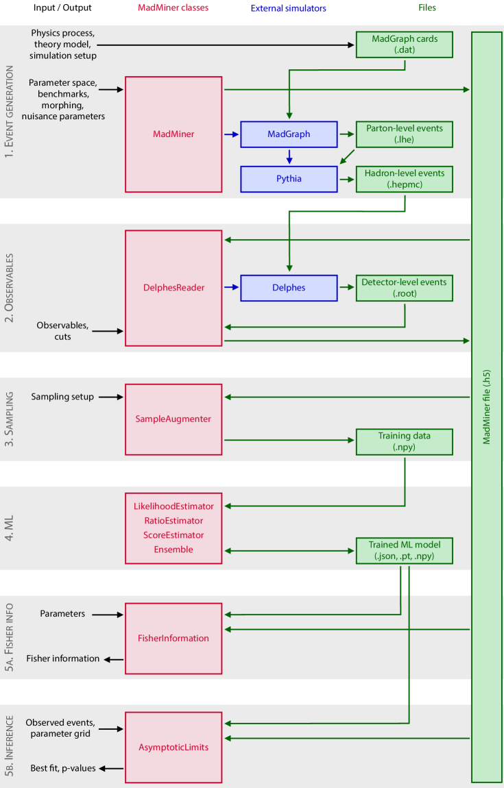
Figure 1: Example workflow, with classes in red, external simulations in blue, and files in green.

III.1 Analysis specification and event generation

The first phase of a MadMiner analysis consists of specifying the problem and generating events. First, the necessary files (“cards”) that define the analyzed process and theoretical model should be collected. This includes the UFO model files as well as the run card, the parameter card, the Pythia card, and the Delphes card, all in the standard format used by MadGraph5_aMC.

The measurement problem is specified with an instance of the MadMiner class. The parameter space is defined by repeatedly calling its add_parameter() function. Each model parameter is specified by its LHA block and LHA ID in the UFO model.

Next, the user chooses benchmarks: parameter points at which the event are evaluated. Benchmarks can be specified manually with add_benchmark(). Additionally, a morphing technique based on Eq. 17 can be activated by calling set_morphing(). If less benchmarks have been manually specified than required for a morphing basis, more benchmarks will be chosen automatically, minimizing the expected size of morphing weights $|w_{c}(x)|$.

Systematic uncertainties (from PDF and scale variations) can be specified with a call to set_systematics(). Once the parameter space, benchmarks, morphing, and systematic uncertainties are set up, save() saves these settings in the MadMiner file, which is based on the HDF5 standard hdf5 .

Finally, events can be generated by calling run() or run_multiple() (the difference is that the former starts one event generation run, while the latter generates multiple sets with different run cards or sampled from different benchmarks). MadMiner will set up MadGraph’s reweighting feature to evaluate the event weights for all events at all benchmarks, which are stored in the LHE event files together with the parton-level information. Pythia 8 will automatically be called to shower and hadronize the partons, the results are stored in a standard HepMC event file Dobbs:2001ck .

III.2 Detector effects and observables

In the second phase, all relevant information has to be extracted from the event samples, including observables as well as event weights for the different benchmarks. There are currently two implementations for this step: the LHEReader class realizes a simple parton-level analysis, in which the effects of shower and detector are approximated with transfer functions, while the DelpesReader class implements an detector-level analysis in which the shower is modeled with Pythia 8 and the detector with Delphes 3. The API of both classes is very similar, here we focus on the DelpesReader option.

After creating a DelphesReader instance and pointing it to the MadMiner file, the user has to list the HepMC event samples that should be analyzed by calling the function add_sample(). The detector simulation with Delphes can either be run externally or through MadMiner by calling run_delphes().

In a next step, the user defines a set of observables that will be calculated for each event. These can be provided either as Python functions with add_observable_from_function() or as parse-able strings with add_observable(). In both cases, reconstructed objects are accessible as MadMinerParticle objects, which inherits all functions of scikit-hep’s LorentzVector class eduardo_rodrigues_2019_3234683 . This makes observable definitions very easy: for instance, the transverse momentum of the hardest lepton can simply be defined as add_observable("lepton_pt", "l[0].pt"), while the azimuthal angle between the two hardest jets can be defined as add_observable("delta_phi", "j[0].deltaphi(j[1])"). Cuts can be added similarly with add_cuts().

Once all samples are added, Delphes has been called, and all observables and cuts are defined, a call to analyse_delphes_samples() parses the observables for the simulated events, applies the cuts, and extracts the relevant event weights. With save() this data is stored in the MadMiner file.

III.3 Sample unweighting and augmentation

If multiple different samples were created, for instance for different processes or phase-space regions, they should now be combined into a single MadMiner file and shuffled by calling the combine_and_shuffle() function.

In the third step of the analysis workflow, the event information in the MadMiner file is processed into training data for the different algorithms described in the previous section. This consists of two aspects: first, the event data needs to be reweighted to the parameter points $\theta$ (and / or $\theta_{0}$, $\theta_{1}$, $\theta_{\text{ref}}$) that make up the training data and then unweighted. Second, the joint likelihood ratio $r(x,z)$ and the joint score $t(x,z)$ need to be calculated for each unweighted event.

This is implemented in the SampleAugmenter class. It provides a set of six high-level functions that generate and augment the data for the different types of inference techniques. For instance, sample_train_local() generates training samples for score estimators (the Sally and Sallino techniques), while sample_train_ratio() prepares training data for likelihood ratio estimators. The output of all these functions are a set of plain NumPy numpy arrays. The rows of these two-dimensional arrays are the events; the columns correspond to the observables that characterize the event data (in the order in which the observables were defined in the DelphesReader or LHEReader classes), the parameter points according which they are sampled, and the components of the joint score, respectively.

III.4 Machine learning

It is finally time to train neural networks to estimate the likelihood, likelihood ratio, or score, as discussed in Sec. II. This is implemented in the classes LikelihoodEstimator, ParameterizedRatioEstimator, DoubleParameterizedRatioEstimator, and ScoreEstimator. This training is independent of the external Monte-Carlo simulations and even the MadMiner file, which makes it easy to run it on an external system with GPU support.

During initialization of any of these classes, the network architecture is chosen. Currently, MadMiner supports fully connected feed-forward networks with variable number of layers, hidden units, and activation functions, implemented in PyTorch paszke2017automatic . A call to train() starts the training; keywords specify which loss function to use, the location of the training data generated in the previous step, the optimizer, the learning rate schedule, the batch size, and whether early stopping is used.

After training, save() saves the neural network to files. The estimators are evaluated for arbitrary parameter points and observables with evaluate_log_likelihood(), evaluate_log_likelihood_ratio(), or evaluate_score(). For many users, the estimates returned by these functions will be the final output of MadMiner, and the statistical analysis will be performed externally.

We also provide the Ensemble class, a convenient wrapper that allows to train an ensemble of multiple neural networks. The different instances can have identical or different architectures and the training can be performed on the same or resampled training data. Such an ensemble is useful for consistency checks and uncertainty estimation as discussed in Sec. II.5.

III.5 Inference

MadMiner provides a barebones framework for the statistical analysis: the AsymptoticLimits class. After initalizing it with the MadMiner file, the two high-level functions expected_limits() and observed_limits() calculate expected and observed $p$-values over a grid in parameter space. expected_limits() takes as input the parameter point that is assumed to be true and internally generates a so-called “Asimov” data set Cowan:2010js , a large simulated set of events. observed_limits() on the other hand is directly based on a list of events, which the user can take from simulations or actual measured data.

Both methods can estimate the kinematic likelihood either through histograms of kinematic variables, through histograms of the estimated score from a trained ScoreEstimator instance, or through a trained likelihood (ratio) estimator. $p$-values are calculated with a likelihood ratio test, using the asymptotic distribution of the likelihood ratio as described in Wilks’ theorem Wilks:1938dza ; Wald ; Cowan:2010js .

The AsymptoticLimits currently does not support systematic uncertainties. We are planning to interface MadMiner with existing software packages that implement profile likelihood ratio tests.

III.6 Fisher information

As discussed in Sec. II.3, a convenient and powerful summary of the sensitivity of a measurement is the Fisher information matrix. Its calculation is implemented in the FisherInformation class. Most importantly, full_information() calculates the Fisher information based on a ScoreEstimator instance as given in Eq. (16). Several other functions allow to calculate the Fisher information in the cross section only (i. e. the first term of Eq. (16)), the Fisher information in the histogram of one or two kinematic variables, and finally the truth-level Fisher information, which treats all properties of the parton-level particles as observable. Finally, the function histogram_of_information() allows the user to calculate the distribution of the Fisher information over phase space, as introduced in Ref. Brehmer:2016nyr .

In the presence of systematic uncertainties and in a frequentist setup, nuisance parameters can either be neglected (“projected out”) or conservatively taken into account (“profiled out”). These operations are implemented in the functions project_information() and profile_information().

IV Physics example

We demonstrate the use of MadMiner in the measurement of dimension-six operators in $tth$ production at the high-luminosity run of the LHC. We choose to analyze fully leptonic top decays and a Higgs decay into two photons,

$$pp\to t\bar{t}\,h\to(b\ell^{+})\,(\bar{b}\ell^{-})\,(\gamma\gamma)\,{E_{T}^{\text{miss}}}$$ (20)

with $\ell=e,\mu$. While this particular signature is not expected to be the most sensitive channel, for example when compared to either semi-leptonic $tth$ production or Higgs production in gluon fusion, it provides a high-dimensional final state with a non-trivial missing energy signature, illustrating the features and challenges that MadMiner can address.

We consider three different scenarios:

Illustration

We first illustrate the mechanism behind the inference techniques in MadMiner in a one-dimensional version of the problem, restricting the analysis to one parameter and one observable.

Validation

MadMiner is then validated in a parton-level toy scenario. By not letting the $W$ bosons decay and ignoring the effect of shower and detector on observables, we can calculate the true likelihood function and compare the output of the neural networks to a ground truth.

Physics analysis

Finally, we perform a realistic phenomenological analysis, including the effects of parton shower and detector and considering a three-dimensional parameter space and high-dimensional event data.

All three analyses are performed with MadMiner v0.4 following the workflow outlined in the previous section. Events are generated with MadGraph5_aMC@NLO at leading order for $\sqrt{s}=14\leavevmode\nobreak\ $\mathrm{T}\mathrm{e}\mathrm{V}$$ using the PDF4LHC15_nlo parton distribution function Butterworth:2015oua . We normalize the rates to the NLO predictions deFlorian:2016spz with a phase-space-independent $k$-factor. We consider the Standard Model Lagrangian supplemented with dimension-six operators in the SILH basis Giudice:2007fh , as implemented in the HEL FeynRules model Alloul:2013naa .

	Illustration	Validation	Physics analysis
Operators	$\mathcal{O}_{G}$	$\mathcal{O}_{u}$, $\mathcal{O}_{G}$, $\mathcal{O}_{uG}$	$\mathcal{O}_{u}$, $\mathcal{O}_{G}$, $\mathcal{O}_{uG}$
Initial states	$pp$	$gg$	$pp$
Final state	$(b\ell^{+})\,(\bar{b}\ell^{-})\,(\gamma\gamma)\,{E_{T}^{\text{miss}}}$	$(bW^{+})\,(\bar{b}W^{-})\,(\gamma\gamma)$	$(b\ell^{+})\,(\bar{b}\ell^{-})\,(\gamma\gamma)\,{E_{T}^{\text{miss}}}$
Background	$\checkmark$	–	$\checkmark$
Shower simulation	Pythia	–	Pythia
Detector simulation	Delphes	–	Delphes
Observables	1: $p_{T,\gamma\gamma}$	80	48
Systematic uncertainties	–	–	PDF, scale

Table 2: The three scenarios in which we analyze the $tth$ process.

Otherwise, the simulation setup is different for each of the three scenarios. We summarize the main settings in Tbl. 2 and discuss them in each of the following sections.

IV.1 Illustration of analysis techniques

Our first analysis aims to illustrate how MadMiner calculates the likelihood function in a simplified one-dimensional version of the problem. For this we restrict ourselves to a single dimension-six operator,

$$\mathcal{L}=\mathcal{L}_{SM}+c_{G}\,\mathcal{O}_{G}$$ (21)

with

$$\mathcal{O}_{G}=\frac{g_{s}^{2}}{m_{W}^{2}}(H^{\dagger}H)G_{\mu\nu}^{a}G_{a}^{\mu\nu}\,.$$ (22)

This operator induces an additional contribution to the effective Higgs-gluon coupling, $g_{ggh}\to g_{ggh}(1+192\pi^{2}/g^{2}\times c_{G})$, and therefore affects the kinematic distributions (Maltoni:2016yxb, ).

We define the theory parameter as $\theta=100\,c_{G}$, which is dimensionless and of order unity over the parameter range of interest. $\theta=0$ then corresponds to the SM, any deviation from zero to a new physics effect. The squared matrix element consists of an SM contribution, an interference term linear in $\theta$, and a squared dimension-six amplitude proportional to $\theta^{2}$, and we can use a morphing technique to interpolate event weights and cross sections from three benchmarks (or morphing basis points) to any point in parameter space.

In this illustration setup we also restrict the analysis to a single observable $x=p_{T,\gamma\gamma}$, the transverse momentum of the di-photon system. All other observables are treated as if they were unobservable. Together with physically unobservable degrees of freedom (such as neutrino energies) as well as random variables in the simulation of the shower, hadronization, and detector, they form the set of latent variables $z$. This setup is similar to a histogram-based analysis of $c_{G}$ using only the $p_{T,\gamma\gamma}$ histogram.

We generate events with MadGraph5_aMC@NLO as described above. They are then showered and hadronized through Pythia 8. The detector response is simulated with Delphes 3 using the HL-LHC card suggested by the HL/HE-LHC working group Cepeda:2019klc .

IV.1.1 Signal only

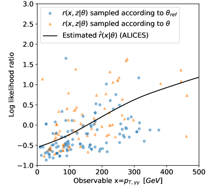
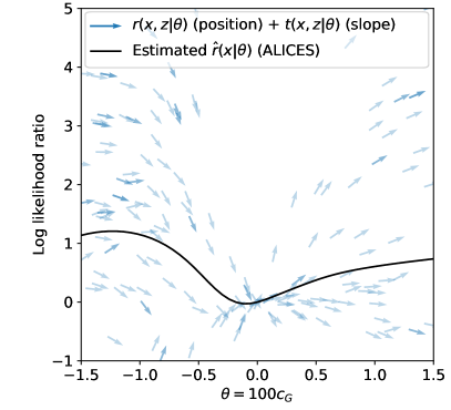
Figure 2: Illustration of the analysis techniques in a one-dimensional problem. Left: Joint log likelihood ratio as a function of the observable $p_{T,\gamma\gamma}$ for $tth$ signal events sampled according to the SM (blue dots) and a BSM theory with $\theta=100\,c_{G}=1$ (orange triangles). The solid line shows the estimated log likelihood ratio from an Alices model trained only on $p_{T\gamma\gamma}$ as input observable. Right: Joint log likelihood ratio (arrow position) and joint score (arrow slope) as a function of the model parameter $\theta=100\,c_{G}$, for $tth$ signal events in the range $p_{T,\gamma\gamma}=(300\pm 2.5)$ GeV. The solid line shows the estimated log likelihood ratio from an Alices model trained only on $p_{T,\gamma\gamma}$ as input observable and evaluated at $p_{T,\gamma\gamma}=300$ GeV.

In the sampling and data augmentation step (the third box in Fig. 1), MadMiner creates training samples where each simulated event is characterized by values of the observable $x=p_{T,\gamma\gamma}$ and the (unobservable) latent variables $z$. Additionally, for each event MadMiner calculates the joint likelihood ratio $r(x,z|\theta)$ between the parameter point $\theta$ and a reference point $\theta_{\text{ref}}$, which we take to be the SM. It also calculates the joint score $t(x,z|\theta)$ evaluated at the parameter point $\theta$. This is illustrated in Fig. 2. The blue dots and orange triangles in the left panel show the joint log likelihood ratio $\log r(x,z|\theta)$ with their dependence on the observable $x=p_{T,\gamma\gamma}$. The blue dots show $tth$ events sampled according to the SM (with $\theta_{\text{ref}}=0$), while the orange triangles are sampled from a BSM hypothesis with $\theta=1$ (or $c_{G}=0.01$). We can see that there are more high-$p_{T}$ events for the BSM model than for the SM, and hence the joint likelihood ratio is higher. The large vertical scatter in the joint likelihood ration is caused by the presence of the latent variables $z$, which affect the joint likelihood ratio, but are unobservable. In the right panel of the same figure, the arrows show the joint log likelihood ratio $\log r(x,z|\theta)$ (arrow position) and the joint score $t(x,z|\theta)$ (arrow slope) with their dependence on the theory parameter $\theta$. Here the observable is constrained to the range $p_{T,\gamma\gamma}=(300\pm 2.5)\leavevmode\nobreak\ $\mathrm{G}\mathrm{e}\mathrm{V}$$ to suppress the observable dependence.

Estimating the likelihood ratio with the methods described in Sec. II.2 (and in more detail in Ref. Brehmer:2018eca ) essentially means fitting a function $\hat{r}(x|\theta)$ to the joint likelihood ratio $r(x,z|\theta)$ by numerically minimizing a suitable loss functions. In this process, the unobservable latent variables $z$ are effectively integrated out. This is the gist of the machine learning step of the MadMiner workflow (box four in Fig. 1). The result of this step, the estimated log likelihood ratio $\hat{r}(x|\theta)$ based on the Alices method, is shown in the solid black lines in Fig. 2: the left panel illustrates the $x$ dependence for fixed $\theta=1$, the right panel the $\theta$ dependence for fixed $x$. While it is possible to estimate the likelihood ratio only using the joint likelihood ratio as input, the gradient information that is the joint score provides additional guidance, which often allows for the fit to converge with less data.

IV.1.2 Adding backgrounds

So far we have only considered the $tth$ signal process. How does this picture change when we include backgrounds? We answer this question in the left panel of Fig. 3, where in addition to the signal we now include the dominant background, continuum $t\bar{t}\,\gamma\gamma$ production with leptonically decaying tops.

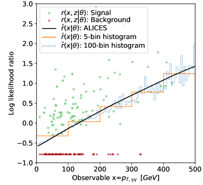
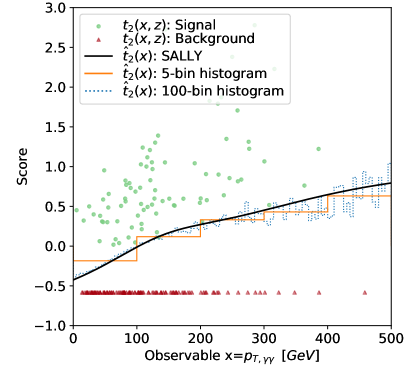
Figure 3: Illustration of the analysis techniques in a one-dimensional problem. Left: Joint log likelihood ratio as a function of the observable $p_{T\gamma\gamma}$ for $tth$ signal events (green dots) and $tt\gamma\gamma$ background events (red triangles) sampled according to the SM and a BSM theory with $\theta=100\leavevmode\nobreak\ c_{G}=1$. The background events cluster at a constant value of $-0.78$, as explained in the text. The lines show the estimated log likelihood ratio based on the Alices method trained only on $p_{T,\gamma\gamma}$ (black solid) and a $p_{T,\gamma\gamma}$ histogram with 5 (orange solid) and 100 (blue dashed) bins, respectively. Right: Joint score evaluated at the SM for for $tth$ signal (green dots) and $tt\gamma\gamma$ background events (red triangles). The background events cluster at a constant value of $-0.58$, as explained in the text. The lines show the estimated score obtained using a Sally method trained only on $p_{T\gamma\gamma}$ (black solid) and a $p_{T,\gamma\gamma}$ histogram with 5 (orange solid) and 100 (blue dashed) bins, respectively.

As before the circles show the joint log likelihood ratio $\log r(x,z|\theta)$ and the line denotes the estimated log likelihood ratio function $\log\hat{r}(x|\theta)$. Since signal and background populate different phase-space regions, the interference between them is negligible and we could consistently simulate them separately from each other. This means that every simulated event is labeled either as a signal or a background event, which plays the role of a discrete variable in the set of latent variables $z$. The background event weights are unaffected by the EFT operator $\mathcal{O}_{G}$, so the joint likelihood ratio for these events is independent of $x$ and $z$:

$$r(x,z|\theta)\bigg{|}_{\text{background}}=\frac{p(x,z|\theta)}{p(x,z|\theta_{\text{ref}})}=\frac{\mathrm{d}\sigma(z_{p}|\theta)}{\mathrm{d}\sigma(z_{p}|\theta_{\text{ref}})}\,\frac{\sigma(\theta_{\text{ref}})}{\sigma(\theta)}=\frac{\sigma(\theta_{\text{ref}})}{\sigma(\theta)}\,,$$ (23)

which in our case turns out to be

$$\log r(x,z|\theta)\bigg{|}_{\text{background}}=-0.78=:\log r^{*}\,.$$ (24)

This is clearly visible in the left panel of Fig. 3, where the $t\bar{t}\,\gamma\gamma$ events show up as a horizontal line at this value. While the presence of backgrounds does not affect the fundamental validity of the inference technique, it increases the variance of the joint likelihood ratio around the true likelihood ratio so that more training events are required before the neural network converges on the true likelihood ratio function.

In this simple example with one-dimensional observations $x$, we can validate the Alices predictions with histograms. The histogram approximation for the likelihood ratio is $\hat{r}(x|\theta)=[\sigma_{\text{bin}}(\theta)/\sigma(\theta)]/[\sigma_{\text{bin}}(\theta_{\text{ref}})/\sigma(\theta_{\text{ref}})]$, where $\sigma_{\text{bin}}(\theta)$ is the cross section in the bin corresponding to $x$. In the left panel of Fig. 3, the log likelihood ratio based on a histogram with 5 (100) equally sized bins is shown as solid orange (dashed blue) line. It generally agrees excellently with the Alices prediction. The two histogram lines show the trade-off in the number of bins: while too few bins lead to large binning effects, a large number of bins can lead to large fluctuations due to limited Monte-Carlo statistics. In contrast, the MadMiner techniques based on neural networks learn the correct continuum limit equivalent to an infinite number of histogram bins, without suffering from large fluctuations.

In Sec. II.3 we described an alternative approach in which MadMiner calculates the score, a vector of summary statistics that are statistically optimal close to a reference parameter point such as the SM. We illustrate this Sally technique in the right panel of Fig. 3. The green circles show the joint score $t(x,z)$ at the SM reference point, corresponding to the change of the log likelihood when infinitesimally increasing the sole theory parameter $\theta=100\,c_{G}$. In analogy to the log likelihood ratio, the red points clustering at a horizontal line

$$t(x,z)\bigg{|}_{\text{background}}=-0.58=:t^{*}$$ (25)

correspond to the $t\bar{t}\,\gamma\gamma$ background events. Estimating the score function conceptually corresponds to fitting a function $\hat{t}(x)$ to the joint score data $t(x,z)$ by numerically minimizing an appropriate loss function. The resulting score estimator $\hat{t}(x)$ is shown as a solid black line. Again, in this one-dimensional case we can compare the result to the score estimated through a histogram, which is shown in a solid red (dashed green) line for a histogram with 5 (100) bins. We find excellent agreement between the Sally prediction and the histogram results.

IV.2 Validation at parton level

Next, we validate MadMiner in a setup in which we can calculate a ground truth for the output of the algorithms. This is not trivial because the ground truth — the true likelihood, likelihood ratio, or score — is intractable in realistic situations. In the last section we showed how we can use histograms to check the algorithms, but only when limiting the analysis to one or two observables. We now turn to another approximation in which we can access the true likelihood ratio and score, even though both observables and model parameters are high-dimensional: Following Ref. Brehmer:2018kdj ; Brehmer:2018eca , we consider a truth-level scenario in which all latent variables are also observable, $x=z$. In this case the likelihood ratio $r(x)$ is equal to the joint likelihood ratio $r(x,z)$ and the score $t(x)$ is equal to the joint score $t(x,z)$. We can thus compare the predictions of a neural network trained to estimate either of these quantities to a ground truth.

For this validation we choose the parton-level process

$$gg\to t\bar{t}h\to(bW^{+})\,(\bar{b}W^{-})\,(\gamma\gamma)\,.$$ (26)

We do not let the $W$ bosons decay and assume that the four-momenta and flavors of all initial-state and final-state particles can be measured, i. e. we do not simulate the effect of parton shower and detector response. These truth-level approximations are not necessary for the inference techniques in MadMiner, but they allow us to calculate a ground truth for the likelihood ratio and score, which is not possible for any realistic treatment of neutrinos or modeling of parton shower and detector response.

Following Ref. Maltoni:2016yxb , we consider three dimension-six operators affecting the top and Higgs couplings in $tth$ production:

$$\mathcal{L}=\mathcal{L}_{SM}+c_{u}\,\mathcal{O}_{u}+c_{G}\,\mathcal{O}_{G}+c_{uG}\,\mathcal{O}_{uG}\,,$$ (27)

where the operators are defined as

$$\mathcal{O}_{u}=-\frac{1}{v^{2}}(H^{\dagger}H)(H^{\dagger}\bar{Q}_{L})u_{R}\,,\ \mathcal{O}_{G}=\frac{g_{s}^{2}}{m_{W}^{2}}(H^{\dagger}H)G_{\mu\nu}^{a}G_{a}^{\mu\nu}\,,\ \mathcal{O}_{uG}=-\frac{4g_{s}}{m_{W}^{2}}y_{u}(H^{\dagger}\bar{Q}_{L})\gamma^{\mu\nu}T_{a}u_{R}G^{a}_{\mu\nu}\,.$$ (28)

The $\mathcal{O}_{u}$ operator effectively rescales the top Yukawa coupling as $y_{t}\to y_{t}\times(1+3/2\times c_{u})$, essentially rescaling the overall rate of the $tth$ process. As discussed in the previous section, the $\mathcal{O}_{G}$ operator induces an additional contribution to the effective Higgs-gluon coupling, $g_{ggh}\to g_{ggh}(1+192\pi^{2}/g^{2}\times c_{G})$, and thus changes the kinematic distributions. Finally, the $\mathcal{O}_{uG}$ operator corresponds to a top-quark chromo-dipole moment, which modifies the $gtt$ vertex. It also induces new effective $ggtt$, $gtth$, and $ggtth$ couplings, promising new kinematic features.

As theory parameters we define the vector

$$\theta=(\theta_{1},\theta_{2},\theta_{3})^{T}=(c_{u},100\,c_{G},100\,c_{uG})^{T}\,,$$ (29)

Two of the Wilson coefficients are rescaled by a factor 100 to make sure that typical values of the three parameters are of the same size. Like in most EFT analyses, the squared matrix element factorizes as described in Eq. 17, and we can use a morphing technique to interpolate event weights and cross sections from nine benchmarks (or morphing basis points) to any point in parameter space.

Based on a sample of $1.25\cdot 10^{6}$ events, we train a likelihood ratio estimator with the Alices technique and a score estimator with the Sally method.

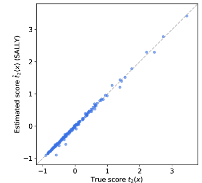
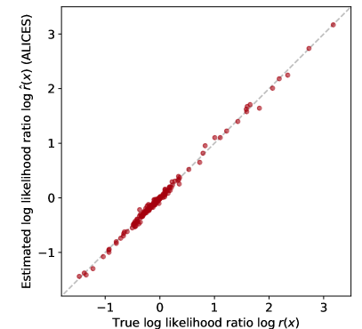
Figure 4: Validation of the analysis techniques in a parton-level analysis, treating the momenta and flavours of all initial-state and final-state partons are observable. Left: Validation of score estimation with the Sally method. Estimated vs. true score component $t_{2}(x)$ evaluated at the SM. Right: Validation of likelihood ratio estimation with the Alices technique. Estimated vs. true log likelihood ratio $\log r(x|\theta)$. The numerator parameter points $\theta$ are drawn from a multivariate Gaussian with mean $(0,0,0)$ and covariance matrix $\operatorname{diag}(0.2^{2},0.2^{2},0.2^{2})$ as an example for a relevant region of parameter space.

We show the results in Fig. 4. The left panel shows the correlation between the true and estimated score based on the Sally technique, focusing on the score component $t_{2}(x)$ that corresponds to the theory parameter $\theta_{2}=100\,c_{G}$ (with similar results for the other components). In the right panel we compare the estimated likelihood ratio based on the Alices method to the ground truth, with parameter points drawn from a region of parameter space that could be of interest in a typical analysis. In both cases we find that the predictions of the neural network are very close to the true values, confirming that the MadMiner algorithms work correctly in this truth-level scenario.

IV.3 Realistic physics analysis

Finally we analyse the new physics reach of the $tth$ process in a realistic setup with high-dimensional event data and theory parameters. We consider the three dimension-six operators given in Eqs. (27) and (28) and define the theory parameter space as in Eq. (29).

In addition to the $tth$ signal we again include the dominant background, continuum $t\bar{t}\,\gamma\gamma$ production with leptonically decaying tops. We take into account that this process is sensitive to the theory parameter $c_{uG}$ through the modified $gtt$ and $ggtt$ vertex while being independent of $c_{u}$ and $c_{G}$. We neglect subleading backgrounds, in particular those with fake photons or fake leptons.

The event generation follows the discussion in Sec. IV.1; we simulate the parton shower with Pythia 8 and the detector response with Delphes 3 using the HL-LHC detector setup. We now also take into account PDF and scale uncertainties, using the 30 eigenvectors of the PDF4LHC15_nlo_30 PDF set and independently varying renormalization and factorization scales by a factor of 2.

The event data is described by 48 observables, which includes the four-momenta of all reconstructed final-state objects (photons, leptons, and jets), the missing energy, as well as derived quantities such as the reconstructed transverse momentum of the di-photon system $p_{T,\gamma\gamma}$. We require the events to pass a di-photon mass cut $115\leavevmode\nobreak\ $\mathrm{G}\mathrm{e}\mathrm{V}$<m_{\gamma\gamma}<135\leavevmode\nobreak\ $\mathrm{G}\mathrm{e}\mathrm{V}$$ and to pass one of four triggers, which were adopted from the Delphes default trigger card: the mono-photon trigger ($p_{T,\gamma}>80\leavevmode\nobreak\ $\mathrm{G}\mathrm{e}\mathrm{V}$$), the di-photon trigger ($p_{T,\gamma_{1}}>40\leavevmode\nobreak\ $\mathrm{G}\mathrm{e}\mathrm{V}$$ and $p_{T,\gamma_{2}}>20\leavevmode\nobreak\ $\mathrm{G}\mathrm{e}\mathrm{V}$$), the mono-lepton tigger ($p_{T,\ell}>29\leavevmode\nobreak\ $\mathrm{G}\mathrm{e}\mathrm{V}$$), or the di-lepton trigger ($p_{T,\ell_{1}}>17\leavevmode\nobreak\ $\mathrm{G}\mathrm{e}\mathrm{V}$$ and $p_{T,\ell_{2}}>17\leavevmode\nobreak\ $\mathrm{G}\mathrm{e}\mathrm{V}$$). For an anticipated integrated luminosity of $\mathcal{L}=3\leavevmode\nobreak\ $\mathrm{a}\mathrm{b}^{-1}$$ at the HL-LHC, we expect 24.5 $tth$ SM signal and 33.6 $tt\gamma\gamma$ background events to pass these acceptance and selection cuts.

We simulate $1.5\cdot 10^{6}$ signal and $10^{6}$ background events (after all cuts) and extract training samples with $10^{7}$ unweighted events. We then train neural networks to estimate the score or likelihood ratio by minimizing the Sally and Alices loss functions, the latter with a hyperparameter $\alpha=0.1$. We use fully connected neural networks with three hidden layers of 100 units and $\tanh$ activation functions, minimize the loss functions with the Adam optimizer using 50 epochs, a batch size of 128, a learning rate that decays exponentially from $10^{-3}$ to $10^{-5}$, and early stopping to avoid overtraining. These hyperparameters are the result of a coarse hyperparameter scan, though we did not perform a exhaustive optimization.

In the final step, we calculate expected exclusion limits and Fisher information matrices. We compare the results of the new methods to a baseline histogram analysis of the transverse momentum of the di-photon system $p_{T,\gamma\gamma}$, and to an analysis of the total cross section alone.

IV.3.1 Fisher information

Following our recommendations from Sec. II.6, we start our physics analysis by using the Sally technique, training a neural network to estimate the score at the SM. We then use it to calculate the SM Fisher information $I_{ij}$ as described in Sec. II.4, finding

$$I_{ij}=\begin{pmatrix}[r]140.5&68.1&170.6\\ 68.1&47.1&105.7\\ 179.5&105.7&283.3\end{pmatrix}\,.$$ (30)

This simple matrix summarizes the sensitivity of the measurement on all three operators. In particular, it allows us to calculate the squared Fisher distance $d^{2}(\theta,\theta_{\text{ref}})=I_{ij}(\theta_{\text{ref}})(\theta-\theta_{\text{ref}})_{i}(\theta-\theta_{\text{ref}})_{j}$. As long as $\theta$ is sufficiently close to $\theta_{\text{ref}}$, $d^{2}$ approximates to $(-2)$ times the expected log likelihood ratio between $\theta$ and $\theta_{\text{ref}}$. That, in turn, can be directly translated into an expected $p$-value with which $\theta$ can be excluded if $\theta_{\text{ref}}$ is true, using the asymptotic properties of the likelihood ratio Wilks:1938dza ; Wald ; Cowan:2010js . In the following we use the Fisher Information to calculate expected limits on a combination of two theory parameters, while fixing the remaining theory parameter to its SM value. In this case, the 68% confidence level contours correspond to a local Fisher distance $d=1.509$ (95% CL corresponds to $d=2.447$, 99% CL to $d=3.034$). We show the resulting expected $68\%$ CL contours in the $c_{G}$–$c_{u}$ plane as solid blue line in the left panel of Fig. 5.

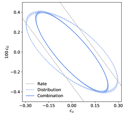
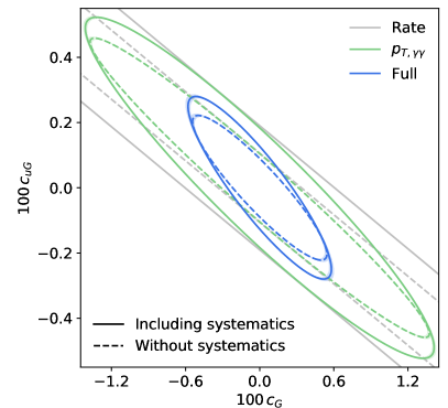
Figure 5: Realistic physics analysis. Left: Expected $68\%$ CL limits in the $c_{G}$–$c_{u}$ plane based on the Fisher information in the rate (gray), the kinematic information (dashed blue), and their combination (solid blue). The kinematic information is calculated based on the Sally technique. The shaded error bands show the ensemble variance of a set of 10 independently trained neural networks. We set $c_{uG}$ to zero. Right: Expected $68\%$ CL limits in the $c_{uG}$–$c_{G}$ plane based on the Fisher Information for the rate (grey), a $p_{T,\gamma\gamma}$ histogram (green), and the full multivariate information based on Sally (blue). The dashed (solid) line shows the reach without (with) systematic uncertainties. The shaded error bands show the ensemble variance of a set of 10 independently trained neural networks. $c_{u}$ is set to zero.

The Fisher information formalism makes it easy to disect these results a little. First, Eq. (16) shows that we can separate the full Fisher information into a rate term and kinematic information. We show this separation in the left panel of Fig. 5 by separately plotting the expected limits corresponding to the rate information (gray), the kinematic information (dashed blue) and their combination (solid blue). We find that kinematic information is crucial for this channel. Since a rate measurement only provides a single number, at the level of the Fisher information it can only constrain one direction in theory space and is blind in the remaining direction. This degeneracy is broken once additional information from the kinematic distributions is included. Indeed, the kinematic information can constrain the rate-sensitive direction in theory space almost as well the rate itself.

Another aspect that can be conveniently discussed in the Fisher information framework are systematic uncertainties. MadMiner can take PDF and scale uncertainties into account by parameterizing them with nuisance parameters and then profiling over them, which at the level of the Fisher information is a simple matrix operation Brehmer:2016nyr ; Edwards:2017mnf . In the right panel of Fig. 5 we analyze the impact of these uncertainties. The dashed lines show the expected limits neglecting systematic uncertainties, while the solid lines show results that take systematics into account by profiling over nuisance parameters. We also again distinguish between the Fisher information in the rate (gray), the Fisher information in a $p_{T,\gamma\gamma}$ histogram (green), and the full information based on a neural score estimator (blue). We can see that the presence of systematic uncertainties, which are dominated by the scale uncertainty, mainly reduces the sensitivity in the rate-sensitive direction. The effect of systematic uncertainties is more pronounced for the information in the total rate and in the $p_{T,\gamma\gamma}$ histogram. The full, multivariate information is reduced mostly in the rate-sensitive direction in parameter space, while the information in the orthogonal direction (to which the rate analysis is blind) is affected only slightly.

The results in both panels of Fig. 5 do not just include central predictions for each Fisher information or contour, but also shaded error bands. These bands visualize the variance of an ensemble of 10 score estimator instances, each trained on resampled training samples with independent random seeds. The bands show $2\sigma$ variations, where $\sigma$ is the ensemble standard deviation for a prediction. The small width of these bands signals a passed sanity check; a larger width would be an indicator for numerical issues during training or insufficient training data.

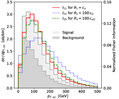
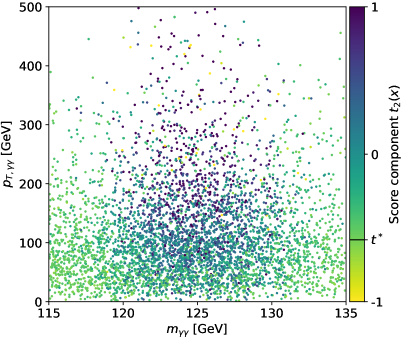
Figure 6: Realistic physics analysis. Left: Differential cross section (shaded grey) and distribution of the Fisher information components (lines) over $p_{T,\gamma\gamma}$. Right: Score component $t_{2}(x)$ corresponding to the Wilson coefficient $c_{G}$ as a function of di-photon mass $m_{\gamma\gamma}$ and di-photon transverse momentum $p_{T,\gamma\gamma}$. Note that events in background-dominated regions cluster at the value $t^{*}=-0.58$, as discussed in Sec. IV.1.

In the discussion so far we have focused on the total Fisher information integrated over phase space, which is related to the expected exclusion limits. There is another useful aspect of the Fisher information: we can analyse the kinematic distribution of the Fisher information over kinematic variables to identify the important phase-space regions for a measurement Brehmer:2016nyr . This knowledge can then be used to design and optimize the event selection. As an example we consider the distribution of information over the di-photon transverse momentum $p_{T,\gamma\gamma}$, which is shown in the left panel of Fig. 6. The shaded grey areas show the differential cross section for the $tt\gamma\gamma$ background and the SM $tth$ signal. The three colored lines show the normalized distribution of the diagonal elements of the Fisher Information. We find that the information on $\mathcal{O}_{u}$, the operator that just rescales the overall $tth$ rate, peaks at $100\leavevmode\nobreak\ $\mathrm{G}\mathrm{e}\mathrm{V}$$, marking the optimal compromise between good signal-to-background ratio and large rate. For $\mathcal{O}_{uG}$ and in particular $\mathcal{O}_{G}$, the information is shifted further towards the high-energy tail of the distribution, where the kinematic effects from these operators are large.

In the right panel of Fig. 6 we illustrate the relation between the score and kinematic variables and show how the score itself can be used to identify the most sensitive region of phase space. We show the score component $t_{2}(x)$, corresponding to the Wilson coefficient $c_{G}$, as a function of the di-photon mass $m_{\gamma\gamma}$ and di-photon transverse momentum $p_{T,\gamma\gamma}$. While the $m_{\gamma\gamma}$ distribution for the signal process does not depend on the Wilson coefficients, this variable is important in telling apart signal and background contributions. As discussed in Sec. IV.1, background events are generated with a constant joint score $t_{2}(x,z)=t^{*}=-0.58$. This is why in kinematic regions dominated by the background, for instance away from the Higgs mass peak, the estimated score approaches a constant value $\hat{t}_{2}(x)\approx t^{*}=-0.58$. Clusters of positive (negative) values of the score component correspond to phase-space regions that are enhanced (suppressed) when increasing $c_{G}$. The largest scores are observed for events around the Higgs peak with high $p_{T,\gamma\gamma}\gtrsim 100\leavevmode\nobreak\ $\mathrm{G}\mathrm{e}\mathrm{V}$$, showing the increased sensitivity of this high-energy region to the Wilson coefficient $c_{G}$. Note that while the score component is clearly related to the two variables shown here, it is not a simple function of $m_{\gamma\gamma}$ and $p_{T,\gamma\gamma}$; the neural network instead learned a non-trivial function of the high-dimensional observable space.

IV.3.2 Exclusion limits

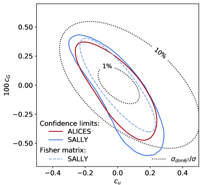
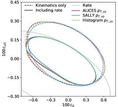
Figure 7: Realistic physics analysis. Left: Comparison of the expected limits in the $c_{G}$–$c_{u}$ plane at 68% CL. We show the limits based on the full likelihood ratio estimated with the Sally (solid blue) and Alices (solid red) methods as well as approximate limits based on the Fisher information calculated with Sally (dashed blue). The dotted black line indicates where the contribution of the dimension-six squared terms contribute 1% and 10% to the total cross section. Right: Comparison of the expected 68% CL exclusion limits in the $c_{uG}$–$c_{G}$ plane using the rate (gray), a $p_{T,\gamma\gamma}$ histogram with 20 bins (green), the Sally method trained with only $p_{T,\gamma\gamma}$ as input (blue), and an Alices likelihood ratio estimator trained with only $p_{T,\gamma\gamma}$ as input (red). The dashed limits only use kinematic distributions, while the solid curves include the rate measurement.

So far we have calculated limits in a local approximation, in which non-linear effects of the theory parameters on the likelihood function are neglected and in which the Fisher information fully characterizes the expected log likelihood ratio as given in Eq. (14). Let us now go beyond this approximation and calculate exclusion limits based on the full likelihood function, including any non-linear effects. In an analysis of effective dimension-six operators, the approach in the previous section corresponds to an analysis of interference effects between the SM contribution and dimension-six effects, while in this section we also take into account the squared dimension-six amplitudes. We can thus draw conclusions about the relevance of the dimension-six squared terms by comparing the limits obtained using the Fisher information with those obtained using the full likelihood ratio function.

In the left panel of Fig. 7 we show the expected 68% CL contours for the parameter plane spanned by $c_{G}$ and $c_{u}$. The solid red line shows the limits obtained using the Alices method, which directly estimates the likelihood ratio function. The Sally method (solid blue line) estimates the SM score vector; the components corresponding to $c_{G}$ and $c_{u}$ are used as observables and the likelihood is calculated with two-dimensional histograms. Finally, the limits based on the local Fisher distance are shown as dashed blue line. We can see the limits obtained using the three methods do not fully agree, indicating the relevance of dimension-six squared terms. Indeed, in the region of parameter space probed at 68% CL, these terms contribute between 1% and 10% to the total rate, as shown by the dotted black lines, and substantially more in the relevant high-energy region of phase space.

These multivariate results are compared to limits based on the analysis of just a single summary statistic in the right panel of Fig. 7. We analyse the $p_{T,\gamma\gamma}$ distribution with three methods: a histogram with 20 bins (pastel green), an Alices likelihood ratio estimator trained only on $p_{T,\gamma\gamma}$ as observable input (forest green), and a Sally estimator of the score trained only on $p_{T,\gamma\gamma}$ as input (turquoise). We also show limits based only on the total cross section (grey) and, for each of the three methods, only on kinematic information (dashed lines). We find that the shape information in the $p_{T,\gamma\gamma}$ distribution (dashed green) is complementary to the rate information, and hence removes the blind directions of the pure rate measurement. In addition, the results from the three methods agree very well, providing a non-trivial cross-check of the three different approaches.

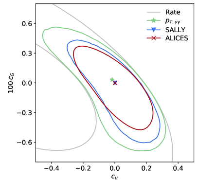
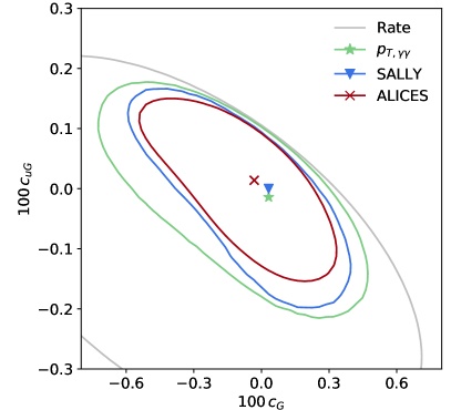
Figure 8: Realistic physics analysis. Expected exclusion limits on the Wilson coefficients $c_{G}$ vs. $c_{u}$ with $c_{uG}$ set to zero (left), and on $c_{uG}$ vs. $c_{G}$ with $c_{u}$ set to zero (right). We show best-fit points and $68\%$ CL limits based on the rate only (gray), a $p_{T,\gamma\gamma}$ histogram with 20 bins (green), the Sally technique (blue), and the Alices method (red).

Finally we collect the expected limits on the Wilson coefficients based on the different methods in Fig. 8. The left panel shows the $c_{G}$–$c_{u}$ plane, the right panel the $c_{uG}$–$c_{u}$ plane, while the parameter not shown is set to zero in both cases. In grey we show limits based on a cut-and-count analysis of the total rate. This approach only constrains one direction in theory space and is blind in the remaining directions. In particular, this rate-only analysis cannot distinguish between multiple disjoint best-fit regions, for instance between $c_{u}=0$ and $c_{u}=-4/3$, which corresponds to a sign-flipped top Yukawa coupling and predicts the same total cross section. This degeneracy is broken once kinematic information is included. Even the simplest case, the histogram-based analysis of a single variable such as the di-photon transverse momentum $p_{T,\gamma\gamma}$ (green line), can substantially improve the sensitivity of the analysis.

The blue and red line show the expected limits from the new, machine-learning-based methods implemented in MadMiner. In blue we show the sensitivity of the Sally technique, which uses the estimated score as a vector of locally optimal observables. We find clearly stronger limits: the score components are indeed more powerful observables than $p_{T,\gamma\gamma}$. Finally, the red line shows the limits from the Alices method, in which a neural network learns the full likelihood ratio function throughout the entire theory parameter space. In contrast to Sally, it also guarantees optimal sensitivity further away from the SM reference point, provided that the network was trained successfully —  and indeed, the Alices technique leads to the strongest expected limits on the Wilson coefficients.

V Conclusions

In this paper we introduced MadMiner, a Python package that implements a range of modern multivariate inference techniques for particle physics processes. These inference methods require running Monte-Carlo simulations and extracting additional information related to the matrix elements, using this information to train neural networks to precisely estimate the likelihood function, and constraining physics parameters based on this likelihood function with established statistical methods. MadMiner implements all steps in this analysis chain.

These inference techniques are designed for high-dimensional event data without requiring a choice of low-dimensional summary statistics. Unlike for instance the matrix element method, they model the effect of a realistic shower and detector simulation, without requiring any approximations on the underlying physics. After an upfront training phase, events can be evaluated extremely fast, which can substantially reduce the computational cost compared to other methods. Finally, the efficient use of matrix element information reduces the number of simulated samples required for a succesful training of the neural networks compared to other, physics-agnostic, machine learning methods.

MadMiner currently provides interfaces to the simulators MadGraph5_aMC, Pythia 8, and the fast detector simulation Delphes 3, which form a state-of-the-art toolbox for phenomenological analyses. It supports almost any LHC process, arbitrary theory models, reducible and irreducible backgrounds, and systematic uncertainties based on PDF and scale variations. In the future, we are planning to extend MadMiner to support detector simulations based on Geant4 as well as new types of systematic uncertainties.

After discussing the implemented inference techniques and their implementation, we provided a step-by-step guide through an analysis workflow with MadMiner. We then demonstrated the tool in an example analysis of three effective operators in $tth$ production at the high-luminosity run of the LHC. The mechanism behind the inference techniques was illustrated in a one-dimensional case, and the methods validated in a simplified parton-level setup where the true likelihood is tractable. We demonstrated how MadMiner lets us isolate the important phase-space regions and define optimal observables. Finally, we showed that compared to analyses of the total rate and standard histograms, the machine-learning-based techniques lead to stronger expected limits on the effective operators. These results demonstrate that the techniques implemented in MadMiner have the potential to clearly improve the sensitivity of the LHC legacy measurements.

Appendix A Frequently asked questions

Here we collect questions that are asked often, hoping to avoid misconceptions:

• Does the whole event history not change when I change parameters?

  No. In probabilistic processes such as those at the LHC, any given event history is typically compatible with different values of the theory parameters, but might be more or less likely. With “event history” we mean the entire evolution of a simulated particle collision, ranging from the initial-state and final-state elementary particles through the parton shower and detector interactions to observables. The joint likelihood ratio and joint score quantify how much more or less likely one particular such evolution of a simulated event becomes when the theory parameters are varied.

• If the network is trained on parton-level matrix element information, how does it learn about the effect of shower and detector?

  It is true that the “labels” that the networks are trained on, the joint likelihood ratio and joint score, are based on parton-level information. But the inputs into the neural network are observables based on a full simulation chain, after parton shower, detector effects, and the reconstruction of observables. It was shown in Ref. Brehmer:2018hga ; Brehmer:2018kdj ; Brehmer:2018eca that the joint likelihood ratio and joint score are unbiased, but noisy, estimators of the true likelihood ratio and true score (including shower and detector effects). A network trained in the right way will therefore learn the effect of shower and detector. We illustrate this mechanism in Sec. IV.1 in a one-dimensional problem.

• Can this approach be used for signal-background classification?

  Yes. In the simplest case, where the signal and background hypothesis do not depend on any additional parameters, the Carl, Rolr, or Alice techniques can be used to learn the probability of an individual event being signal or background. If there are parameters of interest such as a signal strength or the mass of a resonance, the score becomes useful and techniques such as Sally, Rascal, Cascal, and Alices can be more powerful.

  The techniques that use the joint likelihood ratio or score require less training data when the signal and background processes populate the same phase-space regions. If this is not the case, these methods still apply, but will not offer an advantage over the traditional training of binary classifiers.

• What if the simulations do not describe the physics accurately?

  No simulator is perfect, but many of the techniques used for incorporating systematic uncertainties from mismodeling in the case of multivariate classifiers can also be used in this setting. For instance, often the effect of mismodeling can be corrected with simple scale factors and the residual uncertainty incorporated with nuisance parameters. MadMiner can handle such systematic uncertainties as discussed above. If only particular phase-space regions are problematic, for instance those with low-energy jets, we recommend to exclude these parameter regions with suitable selection cuts. If the kinematic distributions are trusted, but the overall normalization is less well known, a data-driven normalization can be used.

  Of course, there is no silver bullet, and if the simulation code is not trustworthy at all in a particular process and the uncertainty cannot be quantified with nuisance parameters, these methods (and many more traditional analysis methods) will not provide accurate results.

• Is the neural network a black box?

  Neural networks are often criticized for their lack of explainability. It is true that the internal structure of the network is not directly interpretable, but in MadMiner the interpretation of what the network is trying to learn is clearly connected to the matrix element. In practical terms, one of the challenges is to verify whether a network has been successfully trained. For that purpose, many cross-checks and diagnostic tools are available to make sure that this is the case:

  • checking the loss function on a separate validation sample;

  • training of multiple network instances with independent random seeds, as discussed above;

  • checking the expectation values of the score and likelihood ratio against their known true values, see Ref. Brehmer:2018eca ;

  • varying of the reference hypothesis in the likelihood ratio, see Ref. Brehmer:2018eca ;

  • training classifiers between data reweighted with the estimated likelihood ratio and original data from a new parameter point, see Ref. Brehmer:2018eca ;

  • validating the inference techniques in low-dimensional problems with histograms, see Sec. IV.1;

  • validating the inference techniques on a parton-level scenario with tractable likelihood function, see Sec. IV.2; and

  • checking the asymptotic distribution of the likelihood ratio against Wilks’ theorem Wilks:1938dza ; Wald ; Cowan:2010js .

  Finally, when limits are set based on the Neyman construction with toy experiments (rather than using the asymptotic properties of the likelihood ratio), there is a coverage guarantee: the exclusion contours constructed in this way will not exclude the true point more often than the confidence level. No matter how wrong the likelihood, likelihood ratio, or score function estimated by the neural network is, the final limits might lose statistical power, but will never be too optimistic.

• Are you trying to replace PhD students with a machine?

  As a preemptive safety measure against scientists being made redundant by automated inference algorithms, we have implemented a number of bugs in MadMiner. It will take skilled physicists to find them, ensuring safe jobs for a while. More seriously, just as MadGraph automated the process of generating events for an arbitrary hard scattering process, MadMiner aims to contribute to the automation of several steps in the inference chain. Both developments enhance the productivity of physicists.

References

- (1) J. Brehmer, K. Cranmer, I. Espejo, F. Kling, G. Louppe, and J. Pavez: ‘Effective LHC measurements with matrix elements and machine learning’, 2019. arXiv:1906.01578.
- (2) K. S. Cranmer: ‘Kernel estimation in high-energy physics’. Comput. Phys. Commun. 136, p. 198, 2001. arXiv:hep-ex/0011057.
- (3) K. Cranmer, G. Lewis, L. Moneta, A. Shibata, and W. Verkerke (ROOT): ‘HistFactory: A tool for creating statistical models for use with RooFit and RooStats’ , 2012.
- (4) M. Frate, K. Cranmer, S. Kalia, A. Vandenberg-Rodes, and D. Whiteson: ‘Modeling Smooth Backgrounds and Generic Localized Signals with Gaussian Processes’ , 2017. arXiv:1709.05681.
- (5) D. B. Rubin: ‘Bayesianly justifiable and relevant frequency calculations for the applied statistician’. Ann. Statist. 12 (4), p. 1151, 1984.
- (6) M. A. Beaumont, W. Zhang, and D. J. Balding: ‘Approximate bayesian computation in population genetics’. Genetics 162 (4), p. 2025, 2002.
- (7) J. Alsing, B. Wandelt, and S. Feeney: ‘Massive optimal data compression and density estimation for scalable, likelihood-free inference in cosmology’ , 2018. arXiv:1801.01497.
- (8) T. Charnock, G. Lavaux, and B. D. Wandelt: ‘Automatic physical inference with information maximizing neural networks’. Phys. Rev. D97 (8), p. 083004, 2018. arXiv:1802.03537.
- (9) J. Brehmer, K. Cranmer, F. Kling, and T. Plehn: ‘Better Higgs boson measurements through information geometry’. Phys. Rev. D95 (7), p. 073002, 2017. arXiv:1612.05261.
- (10) J. Brehmer, F. Kling, T. Plehn, and T. M. P. Tait: ‘Better Higgs-CP Tests Through Information Geometry’. Phys. Rev. D97 (9), p. 095017, 2018. arXiv:1712.02350.
- (11) K. Kondo: ‘Dynamical Likelihood Method for Reconstruction of Events With Missing Momentum. 1: Method and Toy Models’. J. Phys. Soc. Jap. 57, p. 4126, 1988.
- (12) V. M. Abazov et al. (D0): ‘A precision measurement of the mass of the top quark’. Nature 429, p. 638, 2004. arXiv:hep-ex/0406031.
- (13) P. Artoisenet and O. Mattelaer: ‘MadWeight: Automatic event reweighting with matrix elements’. PoS CHARGED2008, p. 025, 2008.
- (14) Y. Gao, A. V. Gritsan, Z. Guo, K. Melnikov, M. Schulze, and N. V. Tran: ‘Spin determination of single-produced resonances at hadron colliders’. Phys. Rev. D81, p. 075022, 2010. arXiv:1001.3396.
- (15) J. Alwall, A. Freitas, and O. Mattelaer: ‘The Matrix Element Method and QCD Radiation’. Phys. Rev. D83, p. 074010, 2011. arXiv:1010.2263.
- (16) S. Bolognesi, Y. Gao, A. V. Gritsan, et al.: ‘On the spin and parity of a single-produced resonance at the LHC’. Phys. Rev. D86, p. 095031, 2012. arXiv:1208.4018.
- (17) P. Avery et al.: ‘Precision studies of the Higgs boson decay channel with MEKD’. Phys. Rev. D87 (5), p. 055006, 2013. arXiv:1210.0896.
- (18) J. R. Andersen, C. Englert, and M. Spannowsky: ‘Extracting precise Higgs couplings by using the matrix element method’. Phys. Rev. D87 (1), p. 015019, 2013. arXiv:1211.3011.
- (19) J. M. Campbell, R. K. Ellis, W. T. Giele, and C. Williams: ‘Finding the Higgs boson in decays to using the matrix element method at Next-to-Leading Order’. Phys. Rev. D87 (7), p. 073005, 2013. arXiv:1301.7086.
- (20) P. Artoisenet, P. de Aquino, F. Maltoni, and O. Mattelaer: ‘Unravelling via the Matrix Element Method’. Phys. Rev. Lett. 111 (9), p. 091802, 2013. arXiv:1304.6414.
- (21) J. S. Gainer, J. Lykken, K. T. Matchev, S. Mrenna, and M. Park: ‘The Matrix Element Method: Past, Present, and Future’. In ‘Proceedings, 2013 Community Summer Study on the Future of U.S. Particle Physics: Snowmass on the Mississippi (CSS2013): Minneapolis, MN, USA, July 29-August 6, 2013’, , 2013. arXiv:1307.3546.
- (22) D. Schouten, A. DeAbreu, and B. Stelzer: ‘Accelerated Matrix Element Method with Parallel Computing’. Comput. Phys. Commun. 192, p. 54, 2015. arXiv:1407.7595.
- (23) T. Martini and P. Uwer: ‘Extending the Matrix Element Method beyond the Born approximation: Calculating event weights at next-to-leading order accuracy’. JHEP 09, p. 083, 2015. arXiv:1506.08798.
- (24) A. V. Gritsan, R. Röntsch, M. Schulze, and M. Xiao: ‘Constraining anomalous Higgs boson couplings to the heavy flavor fermions using matrix element techniques’. Phys. Rev. D94 (5), p. 055023, 2016. arXiv:1606.03107.
- (25) T. Martini and P. Uwer: ‘The Matrix Element Method at next-to-leading order QCD for hadronic collisions: Single top-quark production at the LHC as an example application’ , 2017. arXiv:1712.04527.
- (26) M. Kraus, T. Martini, and P. Uwer: ‘Predicting event weights at next-to-leading order QCD for jet events defined by jet algorithms’ , 2019. arXiv:1901.08008.
- (27) D. Atwood and A. Soni: ‘Analysis for magnetic moment and electric dipole moment form-factors of the top quark via ’. Phys. Rev. D45, p. 2405, 1992.
- (28) M. Davier, L. Duflot, F. Le Diberder, and A. Rouge: ‘The Optimal method for the measurement of tau polarization’. Phys. Lett. B306, p. 411, 1993.
- (29) M. Diehl and O. Nachtmann: ‘Optimal observables for the measurement of three gauge boson couplings in ’. Z. Phys. C62, p. 397, 1994.
- (30) D. E. Soper and M. Spannowsky: ‘Finding physics signals with shower deconstruction’. Phys. Rev. D84, p. 074002, 2011. arXiv:1102.3480.
- (31) D. E. Soper and M. Spannowsky: ‘Finding top quarks with shower deconstruction’. Phys. Rev. D87, p. 054012, 2013. arXiv:1211.3140.
- (32) D. E. Soper and M. Spannowsky: ‘Finding physics signals with event deconstruction’. Phys. Rev. D89 (9), p. 094005, 2014. arXiv:1402.1189.
- (33) C. Englert, O. Mattelaer, and M. Spannowsky: ‘Measuring the Higgs-bottom coupling in weak boson fusion’. Phys. Lett. B756, p. 103, 2016. arXiv:1512.03429.
- (34) Y. Fan, D. J. Nott, and S. A. Sisson: ‘Approximate Bayesian Computation via Regression Density Estimation’. ArXiv e-prints , 2012. arXiv:1212.1479.
- (35) L. Dinh, D. Krueger, and Y. Bengio: ‘NICE: Non-linear Independent Components Estimation’. ArXiv e-prints , 2014. arXiv:1410.8516.
- (36) M. Germain, K. Gregor, I. Murray, and H. Larochelle: ‘MADE: Masked Autoencoder for Distribution Estimation’. ArXiv e-prints , 2015. arXiv:1502.03509.
- (37) K. Cranmer, J. Pavez, and G. Louppe: ‘Approximating Likelihood Ratios with Calibrated Discriminative Classifiers’ , 2015. arXiv:1506.02169.
- (38) K. Cranmer and G. Louppe: ‘Unifying generative models and exact likelihood-free inference with conditional bijections’. J. Brief Ideas , 2016.
- (39) G. Louppe, K. Cranmer, and J. Pavez: ‘carl: a likelihood-free inference toolbox’. J. Open Source Softw. , 2016.
- (40) L. Dinh, J. Sohl-Dickstein, and S. Bengio: ‘Density estimation using Real NVP’. ArXiv e-prints , 2016. arXiv:1605.08803.
- (41) G. Papamakarios and I. Murray: ‘Fast -free Inference of Simulation Models with Bayesian Conditional Density Estimation’. arXiv e-prints arXiv:1605.06376, 2016. arXiv:1605.06376.
- (42) R. Dutta, J. Corander, S. Kaski, and M. U. Gutmann: ‘Likelihood-free inference by ratio estimation’. ArXiv e-prints , 2016. arXiv:1611.10242.
- (43) B. Uria, M.-A. Côté, K. Gregor, I. Murray, and H. Larochelle: ‘Neural Autoregressive Distribution Estimation’. ArXiv e-prints , 2016. arXiv:1605.02226.
- (44) M. U. Gutmann, R. Dutta, S. Kaski, and J. Corander: ‘Likelihood-free inference via classification’. Statistics and Computing p. 1–15, 2017.
- (45) D. Tran, R. Ranganath, and D. M. Blei: ‘Hierarchical Implicit Models and Likelihood-Free Variational Inference’. ArXiv e-prints , 2017. arXiv:1702.08896.
- (46) G. Louppe and K. Cranmer: ‘Adversarial Variational Optimization of Non-Differentiable Simulators’. ArXiv e-prints , 2017. arXiv:1707.07113.
- (47) G. Papamakarios, T. Pavlakou, and I. Murray: ‘Masked Autoregressive Flow for Density Estimation’. ArXiv e-prints , 2017. arXiv:1705.07057.
- (48) J.-M. Lueckmann, P. J. Goncalves, G. Bassetto, K. Öcal, M. Nonnenmacher, and J. H. Macke: ‘Flexible statistical inference for mechanistic models of neural dynamics’. arXiv e-prints arXiv:1711.01861, 2017. arXiv:1711.01861.
- (49) C.-W. Huang, D. Krueger, A. Lacoste, and A. Courville: ‘Neural Autoregressive Flows’. ArXiv e-prints , 2018. arXiv:1804.00779.
- (50) G. Papamakarios, D. C. Sterratt, and I. Murray: ‘Sequential Neural Likelihood: Fast Likelihood-free Inference with Autoregressive Flows’. ArXiv e-prints , 2018. arXiv:1805.07226.
- (51) J.-M. Lueckmann, G. Bassetto, T. Karaletsos, and J. H. Macke: ‘Likelihood-free inference with emulator networks’. arXiv e-prints arXiv:1805.09294, 2018. arXiv:1805.09294.
- (52) T. Q. Chen, Y. Rubanova, J. Bettencourt, and D. K. Duvenaud: ‘Neural ordinary differential equations’. CoRR abs/1806.07366, 2018. arXiv:1806.07366.
- (53) D. P. Kingma and P. Dhariwal: ‘Glow: Generative Flow with Invertible 1x1 Convolutions’. arXiv e-prints arXiv:1807.03039, 2018. arXiv:1807.03039.
- (54) W. Grathwohl, R. T. Q. Chen, J. Bettencourt, I. Sutskever, and D. Duvenaud: ‘FFJORD: Free-form Continuous Dynamics for Scalable Reversible Generative Models’. ArXiv e-prints , 2018. arXiv:1810.01367.
- (55) T. Dinev and M. U. Gutmann: ‘Dynamic Likelihood-free Inference via Ratio Estimation (DIRE)’. arXiv e-prints arXiv:1810.09899, 2018. arXiv:1810.09899.
- (56) J. Hermans, V. Begy, and G. Louppe: ‘Likelihood-free MCMC with Approximate Likelihood Ratios’ , 2019. arXiv:1903.04057.
- (57) J. Alsing, T. Charnock, S. Feeney, and B. Wandelt: ‘Fast likelihood-free cosmology with neural density estimators and active learning’ , 2019. arXiv:1903.00007.
- (58) D. S. Greenberg, M. Nonnenmacher, and J. H. Macke: ‘Automatic Posterior Transformation for Likelihood-Free Inference’. arXiv e-prints arXiv:1905.07488, 2019. arXiv:1905.07488.
- (59) J. Brehmer, G. Louppe, J. Pavez, and K. Cranmer: ‘Mining gold from implicit models to improve likelihood-free inference’ , 2018. arXiv:1805.12244.
- (60) J. Brehmer, K. Cranmer, G. Louppe, and J. Pavez: ‘Constraining Effective Field Theories with Machine Learning’. Phys. Rev. Lett. 121 (11), p. 111801, 2018. arXiv:1805.00013.
- (61) J. Brehmer, K. Cranmer, G. Louppe, and J. Pavez: ‘A Guide to Constraining Effective Field Theories with Machine Learning’. Phys. Rev. D98 (5), p. 052004, 2018. arXiv:1805.00020.
- (62) M. Stoye, J. Brehmer, G. Louppe, J. Pavez, and K. Cranmer: ‘Likelihood-free inference with an improved cross-entropy estimator’ , 2018. arXiv:1808.00973.
- (63) J. Alwall, R. Frederix, S. Frixione, et al.: ‘The automated computation of tree-level and next-to-leading order differential cross sections, and their matching to parton shower simulations’. JHEP 07, p. 079, 2014. arXiv:1405.0301.
- (64) T. Sjostrand, S. Mrenna, and P. Z. Skands: ‘A Brief Introduction to PYTHIA 8.1’. Comput. Phys. Commun. 178, p. 852, 2008. arXiv:0710.3820.
- (65) J. de Favereau, C. Delaere, P. Demin, et al. (DELPHES 3): ‘DELPHES 3, A modular framework for fast simulation of a generic collider experiment’. JHEP 02, p. 057, 2014. arXiv:1307.6346.
- (66) S. Agostinelli et al. (GEANT4): ‘GEANT4: A Simulation toolkit’. Nucl. Instrum. Meth. A506, p. 250, 2003.
- (67) K. Cranmer: ‘Practical Statistics for the LHC’. In ‘Proceedings, 2011 European School of High-Energy Physics (ESHEP 2011): Cheile Gradistei, Romania, September 7-20, 2011’, p. 267-308, 2015. [,247(2015)], arXiv:1503.07622.
- (68) P. Baldi, K. Cranmer, T. Faucett, P. Sadowski, and D. Whiteson: ‘Parameterized neural networks for high-energy physics’. Eur. Phys. J. C76 (5), p. 235, 2016. arXiv:1601.07913.
- (69) S. S. Wilks: ‘The Large-Sample Distribution of the Likelihood Ratio for Testing Composite Hypotheses’. Annals Math. Statist. 9 (1), p. 60, 1938.
- (70) A. Wald: ‘Tests of statistical hypotheses concerning several parameters when the number of observations is large’. Transactions of the American Mathematical Society 54 (3), p. 426, 1943.
- (71) G. Cowan, K. Cranmer, E. Gross, and O. Vitells: ‘Asymptotic formulae for likelihood-based tests of new physics’. Eur. Phys. J. C71, p. 1554, 2011. [Erratum: Eur. Phys. J. C73, p. 2501, 2013]. arXiv:1007.1727.
- (72) J. Alsing and B. Wandelt: ‘Generalized massive optimal data compression’. Mon. Not. Roy. Astron. Soc. 476 (1), p. L60, 2018. arXiv:1712.00012.
- (73) B. Efron: ‘Defining the curvature of a statistical problem (with applications to second order efficiency)’. Ann. Statist. 3 (6), p. 1189, 1975.
- (74) S.-I. Amari: ‘Differential geometry of curved exponential families-curvatures and information loss’. Ann. Statist. 10 (2), p. 357, 1982.
- (75) J. Brehmer: ‘New Ideas for Effective Higgs Measurements’. Ph.D. thesis, U. Heidelberg (main), 2017. URL http://www.thphys.uni-heidelberg.de/~plehn/includes/theses/brehmer_d.pdf.
- (76) C. Radhakrishna Rao: ‘Information and the accuracy attainable in the estimation of statistical parameters’. Bull. Calcutta Math. Soc. 37, p. 81, 1945.
- (77) H. Cramér: ‘Mathematical Methods of Statistics’. Princeton University Press, 1946, ISBN 0691080046.
- (78) T. D. P. Edwards and C. Weniger: ‘A Fresh Approach to Forecasting in Astroparticle Physics and Dark Matter Searches’. JCAP 1802 (02), p. 021, 2018. arXiv:1704.05458.
- (79) C. Degrande, C. Duhr, B. Fuks, D. Grellscheid, O. Mattelaer, and T. Reiter: ‘UFO - The Universal FeynRules Output’. Comput. Phys. Commun. 183, p. 1201, 2012. arXiv:1108.2040.
- (80) O. Mattelaer: ‘On the maximal use of Monte Carlo samples: re-weighting events at NLO accuracy’. Eur. Phys. J. C76 (12), p. 674, 2016. arXiv:1607.00763.
- (81) G. Aad et al. (ATLAS): ‘A morphing technique for signal modelling in a multidimensional space of coupling parameters’, 2015. Physics note ATL-PHYS-PUB-2015-047. URL http://cds.cern.ch/record/2066980.
- (82) J. Alsing and B. Wandelt: ‘Nuisance hardened data compression for fast likelihood-free inference’ , 2019. arXiv:1903.01473.
- (83) Lukas, M. Feickert, G. Stark, R. Turra, and J. Forde: ‘diana-hep/pyhf v0.0.15’, 2018. URL https://doi.org/10.5281/zenodo.1464139.
- (84) R. Frederix, S. Frixione, V. Hirschi, F. Maltoni, R. Pittau, and P. Torrielli: ‘Four-lepton production at hadron colliders: aMC@NLO predictions with theoretical uncertainties’. JHEP 02, p. 099, 2012. arXiv:1110.4738.
- (85) A. Paszke, S. Gross, S. Chintala, et al.: ‘Automatic differentiation in pytorch’. In ‘NIPS-W’, , 2017.
- (86) N. Qian: ‘On the momentum term in gradient descent learning algorithms’. Neural Netw. 12 (1), p. 145, 1999.
- (87) D. P. Kingma and J. Ba: ‘Adam: A Method for Stochastic Optimization’. arXiv e-prints arXiv:1412.6980, 2014. arXiv:1412.6980.
- (88) S. J. Reddi, S. Kale, and S. Kumar: ‘On the convergence of adam and beyond’. In ‘International Conference on Learning Representations’, , 2018.
- (89) B. Lakshminarayanan, A. Pritzel, and C. Blundell: ‘Simple and Scalable Predictive Uncertainty Estimation using Deep Ensembles’. arXiv e-prints arXiv:1612.01474, 2016. arXiv:1612.01474.
- (90) J. Brehmer, F. Kling, I. Espejo, and K. Cranmer: ‘MadMiner code repository’. DOI:10.5281/zenodo.1489147, URL https://github.com/diana-hep/madminer.
- (91) J. Brehmer, F. Kling, I. Espejo, and K. Cranmer: ‘MadMiner technical documentation’. URL https://madminer.readthedocs.io/en/latest/.
- (92) I. Espejo, J. Brehmer, and K. Cranmer: ‘MadMiner Docker repositories’. URL https://hub.docker.com/u/madminertool.
- (93) T. Šimko, L. Heinrich, H. Hirvonsalo, D. Kousidis, and D. Rodríguez: ‘REANA: A System for Reusable Research Data Analyses’. Technical Report CERN-IT-2018-003, CERN, Geneva, 2018. URL https://cds.cern.ch/record/2652340.
- (94) I. Espejo, J. Brehmer, F. Kling, and K. Cranmer: ‘MadMiner Reana deployment’. URL https://github.com/irinaespejo/workflow-madminer.
- (95) The HDF Group: ‘Hierarchical data format version 5’, 2000-2010. URL http://www.hdfgroup.org/HDF5.
- (96) M. Dobbs and J. B. Hansen: ‘The HepMC C++ Monte Carlo event record for High Energy Physics’. Comput. Phys. Commun. 134, p. 41, 2001.
- (97) E. Rodrigues, M. Marinangeli, B. Pollack, et al.: ‘scikit-hep/scikit-hep: scikit-hep-0.5.1’, 2019. URL https://doi.org/10.5281/zenodo.3234683.
- (98) T. Oliphant: ‘NumPy: A guide to NumPy’. USA: Trelgol Publishing, 2006–. URL http://www.numpy.org/.
- (99) J. Butterworth et al.: ‘PDF4LHC recommendations for LHC Run II’. J. Phys. G43, p. 023001, 2016. arXiv:1510.03865.
- (100) D. de Florian et al. (LHC Higgs Cross Section Working Group): ‘Handbook of LHC Higgs Cross Sections: 4. Deciphering the Nature of the Higgs Sector’ , 2016. arXiv:1610.07922.
- (101) G. F. Giudice, C. Grojean, A. Pomarol, and R. Rattazzi: ‘The Strongly-Interacting Light Higgs’. JHEP 06, p. 045, 2007. arXiv:hep-ph/0703164.
- (102) A. Alloul, B. Fuks, and V. Sanz: ‘Phenomenology of the Higgs Effective Lagrangian via FEYNRULES’. JHEP 04, p. 110, 2014. arXiv:1310.5150.
- (103) F. Maltoni, E. Vryonidou, and C. Zhang: ‘Higgs production in association with a top-antitop pair in the Standard Model Effective Field Theory at NLO in QCD’. JHEP 10, p. 123, 2016. arXiv:1607.05330.
- (104) M. Cepeda et al. (Physics of the HL-LHC Working Group): ‘Higgs Physics at the HL-LHC and HE-LHC’ , 2019. arXiv:1902.00134.
- (105) T. Plehn, P. Schichtel, and D. Wiegand: ‘Where boosted significances come from’. Phys. Rev. D89 (5), p. 054002, 2014. arXiv:1311.2591.
- (106) F. Kling, T. Plehn, and P. Schichtel: ‘Maximizing the significance in Higgs boson pair analyses’. Phys. Rev. D95 (3), p. 035026, 2017. arXiv:1607.07441.
- (107) D. Gonçalves, T. Han, F. Kling, T. Plehn, and M. Takeuchi: ‘Higgs boson pair production at future hadron colliders: From kinematics to dynamics’. Phys. Rev. D97 (11), p. 113004, 2018. arXiv:1802.04319.
- (108) D. Merkel: ‘Docker: Lightweight linux containers for consistent development and deployment’. Linux J. 2014 (239), 2014. URL http://dl.acm.org/citation.cfm?id=2600239.2600241.
- (109) T. Kluyver, B. Ragan-Kelley, F. Pérez, et al.: ‘Jupyter notebooks - a publishing format for reproducible computational workflows’. In ‘ELPUB’, , 2016.
- (110) J. D. Hunter: ‘Matplotlib: A 2d graphics environment’. Computing in Science & Engineering 9 (3), p. 90, 2007.
- (111) Lukas: ‘lukasheinrich/pylhe v0.0.4’, 2018. URL https://doi.org/10.5281/zenodo.1217032.
- (112) T. Sjstrand, S. Ask, J. R. Christiansen, et al.: ‘An Introduction to PYTHIA 8.2’. Comput. Phys. Commun. 191, p. 159, 2015. arXiv:1410.3012.
- (113) G. Van Rossum and F. L. Drake Jr: ‘Python tutorial’. Centrum voor Wiskunde en Informatica Amsterdam, The Netherlands, 1995.
- (114) E. Rodrigues: ‘The Scikit-HEP Project’. In ‘23rd International Conference on Computing in High Energy and Nuclear Physics (CHEP 2018) Sofia, Bulgaria, July 9-13, 2018’, , 2019. arXiv:1905.00002.
- (115) F. Pedregosa, G. Varoquaux, A. Gramfort, et al.: ‘Scikit-learn: Machine learning in Python’. Journal of Machine Learning Research 12, p. 2825, 2011.
- (116) J. Pivarski, P. Das, D. Smirnov, et al.: ‘scikit-hep/uproot: 3.7.2’, 2019. URL https://doi.org/10.5281/zenodo.3256257.
- (117) L. Heinrich and K. Cranmer: ‘diana-hep/yadage v0.12.13’, 2017. URL https://doi.org/10.5281/zenodo.1001816.