Interferometric Fringe Visibility Null as a Function of Spatial Frequency: a Probe of Stellar Atmospheres

Abstract

We introduce an observational tool based on visibility nulls in optical spectro-interferometry fringe data to probe the structure of stellar atmospheres. In a preliminary demonstration, we use both Navy Precision Optical Interferometer (NPOI) data and stellar atmosphere models to show that this tool can be used, for example, to investigate limb darkening.

Using bootstrapping with either multiple linked baselines or multiple wavelengths in optical and infrared spectro-interferometric observations of stars makes it possible to measure the spatial frequency $u_{0}$ at which the real part of the fringe visibility ${\rm Re}(V)$ vanishes. That spatial frequency is determined by $u_{0}=B_{\perp}/\lambda_{0}$, where $B_{\perp}$ is the projected baseline length, and $\lambda_{0}$ is the wavelength at which the null is observed. Since $B_{\perp}$ changes with the Earth’s rotation, $\lambda_{0}$ also changes. If $u_{0}$ is constant with wavelength, $\lambda_{0}$ varies in direct proportion to $B_{\perp}$. Any departure from that proportionality indicates that the brightness distribution across the stellar disk varies with wavelength via variations in limb darkening, in the angular size of the disk, or both.

In this paper, we introduce the use of variations of $u_{0}$ with $\lambda$ as a means of probing the structure of stellar atmospheres. Using the equivalent uniform disk diameter $\theta_{\rm UD,0}(\lambda_{0})$, given by $\theta_{\rm UD,0}=1.22/u_{0}(\lambda_{0})$, as a convenient and intuitive parameterization of $u_{0}(\lambda_{0})$, we demonstrate this concept by using model atmospheres to calculate the brightness distribution for $\nu$ Ophiuchi and predict $\theta_{\rm UD,0}(\lambda_{0})$, and then comparing the predictions to coherently averaged data from observations taken with the NPOI.

1 Introduction

In 1891, Michelson placed a two-slit mask across the aperture of the 12-inch telescope on Mt. Hamilton and used it to observe Jupiter’s Galilean satellites. Light passing through the slits from the satellite being observed produced interference fringes in the focal plane. Michelson widened the slit separation until the fringe contrast (the “visibility”) went to zero (Michelson, 1891), thereby producing a measure of the satellite’s angular diameter: the spatial frequency at $u_{0}$ which the fringes vanished, given by $u_{0}=\lambda\,/\,S_{0}$, where $S_{0}$ is the slit separation producing zero visibility, and $\lambda$ is the observing wavelength. Three decades later, he applied this method to stellar observations at Mt. Wilson (Michelson & Pease, 1921), using outrigger mirrors on the 100-inch telescope in place of a mask with slits.

While measuring stellar angular diameters has become one of the primary activities in optical and infrared interferometry — results over the past quarter century in the optical, near-IR, and mid-IR include angular measurements of the pulsations of Cepheids (e.g., Lane et al., 2000; Gallenne et al., 2018) and of their extended envelopes (e.g., Kervella et al., 2006), Be star disks (e.g., Mourard et al., 1989; Gies et al., 2007), and debris disks (e.g., Absil et al., 2006; Ertel et al., 2014), as well as diameter surveys, most recently Baines et al. (2018) — we focus here on developing another use for $u_{0}$: using its variation with wavelength as a probe of the stellar atmosphere.

To set the stage for this idea, consider that most interferometric diameter measurements amount to measuring the fringe visibility amplitude $V$ at one or more spatial frequencies $u$ and using a model fit, usually a uniform disk, to the data to infer the uniform disk diameter $\theta_{UD}$. Here, $u=B_{\perp}\,/\,\lambda$, where $B_{\perp}$ is the component of the interferometer baseline perpendicular to the direction to the star. Conceptually, this method is equivalent to extrapolating $V(u)$ to the spatial frequency $u_{0}$ at which the visibility of a uniformly bright disk vanishes. One then calculates the uniform-disk diameter $\theta_{UD}$ in radians via

$$\theta_{UD}=1.22\,/\,u_{0}.$$ (1)

Since most stars, later types in particular, exhibit a significant amount of limb darkening, investigators have usually estimated the actual diameter of the limb-darkened disk, $\theta_{LD}$, by applying a correction based on models that characterize limb darkening with a few parameters. In a few cases, a limb-darkened disk model, again generated from a parameterized model, is fit directly to the data; see Baines et al. (2018) for examples.

In principle, $u_{0}$, and hence $\theta_{UD}$, are functions of $\lambda$; in fact, some studies, (e.g., Mozurkewich et al., 2003), have used the differences in $\theta_{UD}$ between spectral bands as a means of evaluating a limb darkening model. It is the wavelength dependence of $u_{0}$ that we investigate here as a tool for characterizing stellar atmospheres.

2 The visibility null

Although Michelson found the visibility null itself in his Mt. Hamilton and Mt. Wilson work, most interferometric diameter measurements are made at spatial frequencies smaller than $u_{0}$ and in effect are extrapolated to estimate $u_{0}$, as mentioned above. Jorgensen et al. (2010) and Armstrong et al. (2012) called attention to the fact that one can measure, rather than estimate, $u_{0}$ by observing across the range of $u$ in which $V(u)$, or more precisely, ${\rm Re}[V(u)]$, goes from positive to negative. We can do so, despite having no fringe contrast at $u_{0}$ to enable fringe tracking, if there is enough signal to track fringes simultaneously at longer wavelengths (where $u<u_{0}$) (“wavelength bootstrapping”), or if the fringe on the zero-crossing baseline is stabilized by fringe tracking on shorter baselines (“baseline bootstrapping”).

Jorgensen et al. (2010) showed baseline-bootstrapped examples for three bright stars observed with the Navy Precision Optical Interferometer (NPOI; Armstrong et al., 1998; van Belle et al., 2018). They fitted uniform-disk models to the data near the zero crossings and used those fits to interpolate the wavelength $\lambda_{0}$ at which ${\rm Re}[V(u)]=0$, which yields $u_{0}$ via

$$u_{0}=B_{\perp}/\lambda_{0}.$$ (2)

This method recapitulates Michelson: he too sought the null ($V^{2}=0$ in his case, rather than ${\rm Re}[V(u)]=0$), although he did so by measuring in effect across a range of $B_{\perp}$ rather than a range of $\lambda$. The result in both cases is a measurement of $\theta_{UD}$ via Eq. 1. Jorgensen et al. (2010) obtained $\theta_{UD}$ results with uncertainties ranging from 0.8% to 0.08%. This level of precision is possible because finding $u_{0}$, and hence $\theta_{UD}$, directly is insensitive to multiplicative errors in visibility calibration. For comparison, if one calculates $\theta_{UD}$ using data where $V^{2}$ is no smaller than $0.4$, a 1% error in calibration corresponds to a 0.5% error in $\theta_{UD}$.

This approach offers the possibility of revealing detailed stellar atmosphere information as a function of wavelength. As the Earth rotates, $B_{\perp}$ also changes. As a result, $u_{0}$ also changes because of its dependence on both $B_{\perp}$ (Eq. 2) and any variation in $\theta_{UD}$ with $\lambda$. It is convenient to parameterize the result as $\theta_{UD,0}(\lambda_{0})$, the uniform disk diameter (“UD”) generated from the visibility zero crossing (“0”) as a function of the wavelength $\lambda_{0}$ at which the zero crossing was observed:

$$\theta_{UD,0}(\lambda_{0}) = 1.22\,/\,u_{0}(\lambda)$$ (3)

$$= 1.22\,\lambda_{0}/B_{\perp}.$$

Any variation of $\theta_{UD,0}$ with wavelength is an indication that limb darkening, the effective diameter of the stellar atmosphere, or both, vary with wavelength as well. We may not have gained access to a clear single value of the limb-darkened (LD) diameter, but by treating $\theta_{UD,0}(\lambda_{0})$ as a wavelength-dependent parameter, we have gained a probe of the stellar atmosphere.

3 NPOI data

The NPOI (Armstrong et al., 1998; van Belle et al., 2018) is an optical interferometer located at the Lowell Observatory site on Anderson Mesa, near Flagstaff, Arizona. It includes 10 siderostats: four of them, in fixed locations, form the astrometric subarray, and the other six, which can be moved among 30 stations, form the imaging subarray. The stations are located along the arms of a Y-shaped feed system, each arm of which is $\sim 250$ m long. The array stations provide baseline lengths ranging from 2.2 m to 437 m, although the baselines that have been commissioned to date range from 9 m to 98 m. The current array apertures use 12.5 cm of each 50 cm diameter siderostat, but three 1 m telescopes are currently being installed.

Light is fed from each siderostat or telescope through vacuum feed pipes to the optics laboratory, where optical path differences (OPDs) between array elements due to array geometry and atmospheric turbulence are compensated in continuously-variable vacuum delay lines. In addition to OPD compensation, the delay lines impose 1 kHz triangle-wave delay dithers on each beam line, which modulate the OPDs, thereby scanning over the fringe packets. In the NPOI Classic beam combiner, the combined beams are dispersed into 16 channels spanning $\lambda\lambda$850–520 nm and detected synchronously by cooled avalanche photodiodes in Geiger mode. The VISION beam combiner (Ghasempour et al., 2012; Garcia et al., 2016), currently being commissioned, will dispense with the delay dither by using spatial, rather than temporal, modulation.

The usual observing sequence alternates between a scan on a program target and a scan on a nearby calibrator whose diameter has been measured or can be accurately estimated based on its magnitude and colors. Scans are typically 3 min in length. Depending on the number of stars in the input observing list and other factors, as many as a dozen scans per night can be taken on a given target.

We demonstrate our method with five 30 s scans on $\nu$ Ophiuchi (G9 III) taken with the NPOI on 2005 June 29 (Jorgensen et al., 2010; Armstrong et al., 2012). The observations were taken with the W7, AC, AE, and E6 stations in 16 spectral channels. With the AC station as the group delay tracking reference station, we bootstrapped the 64.4 m W7–AE baseline from the shorter W7–AC and AC–AE baselines and the 79.4 m W7–E6 baseline from the shorter W7–AC and AC–E6 baselines. Bootstrapping plus coherent averaging produced high-SNR data at spatial frequencies spanning ${\rm Re}(V)=0$ on both of these longer baselines. Figure 1 shows the coherently averaged ${\rm Re}[V(\lambda)]$ results.

The curves drawn through the data represent the best-fit uniform disk models multiplied by a wavelength-dependent reduction factor due to phase noise in the data (Jorgensen et al., 2010). In each panel, we indicate the projected baseline toward $\nu$ Oph at the time of the observation; in addition, we show $\lambda_{0}$ and its uncertainty as estimated from the four to six visibility measurements straddling $\lambda_{0}$ and the uniform disk diameter $\theta_{UD,0}$ that produces ${\rm Re}[V(\lambda_{0})]=0$ for baseline length $B_{\perp}$. Note that $\sigma(\lambda_{0})$ is considerably greater for data taken on the W7–AE baseline than on the W7–E6 baseline for two reasons: the slope of ${\rm Re}(V)$ versus $\lambda$ is smaller in the W7–AE data, and the visibilities at the shorter wavelengths are noisier, as is generally true in NPOI data.

To first order, the difference between $\lambda_{0}$ values measured on the W7–AE baseline and those on the W7–E6 baseline are due the difference in $B_{\perp}$ values: shorter baselines require shorter wavelengths to resolve a given stellar diameter. However, the zero-crossing tool, in the form of the $\theta_{UD,0}$ values calculated from $\lambda_{0}$ and $B_{\perp}$, shows that another effect – limb darkening in this case – is also affecting the results.

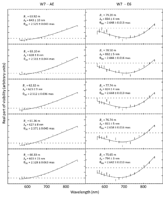
Figure 1: Plots of ${\rm Re}[V(\lambda)]$ for five coherently averaged scans of $\nu$ Ophiuchi (G9 III) during 2005 June 29 using the bootstrapped W7–AE and W7–E6 baselines of the NPOI. The solid lines represent uniform-disk models multiplied by a wavelength-dependent reduction due to phase noise in the data. Vertical bars show $\pm 1\sigma$ uncertainties. As the projected baseline $B_{\perp}$ changes with Earth rotation, the wavelength $\lambda_{0}$ at which ${\rm Re}(V)=0$ changes from scan to scan.

4 Model calculations

In order to compare these data with the predictions from model atmospheres, we first calculate model visibilities with the baselines and wavelength range used in the NPOI observations. Guided by values for $T_{\rm eff}$ ($4831$ K), $\log g$ (2.7), and [Fe/H] (0.1) from Massarotti et al. (2007); Allende Prieto & Lambert (1999) and McWilliam (1990), respectively, we used Kurucz’s brightness profile for a plane-parallel atmosphere ip01k2.pck (“p01” implies ${\rm[Fe/H]=+0.1}$) and extracted the model data for $\log g=2.50$ and $T_{\rm eff}=4750$ K. Kurucz gives the brightness data at 17 values of $\mu$, the cosine of the angle between the normal to the stellar surface and the line of sight, and for every 2 nm in wavelength in the visual range. We expanded the grid to 31 values of $\mu$ by linear interpolation. Selecting an angular diameter for the star effectively converts the radius $r=\sqrt{1-\mu^{2}}$ of an annulus on the stellar disk to angular units. For a range of angular diameters, we calculated the Fourier transform at each wavelength by

$${\rm Re}[V(\lambda)]=\frac{F(\lambda)}{V_{0}}\sum_{i}r_{i}J_{0}\left(\frac{2\pi B_{\perp}r_{i}}{\lambda}\right)\delta r_{i},$$ (4)

where $F(\lambda)$ is the intensity at wavelength $\lambda$, $V_{0}$ is the total flux, which serves to normalize the visibility to unity at zero baseline, $r_{i}$ and $\delta r_{i}$ are the angular radius and thickness of annulus $i$ on the stellar disk, and $J(\cdot)$ is the Bessel function of the first kind and zeroth order. The input diameter that gives the best agreement with the observed visibility near 800 nm is 2.83 mas (see §5). The resulting model ${\rm Re}[V(\lambda)]$ curves are shown in Fig. 2. Note that the angular diameter in this procedure is not a uniform disk diameter, but an actual diameter, at least to the extent that it can reproduce the run of visibilities with wavelength.

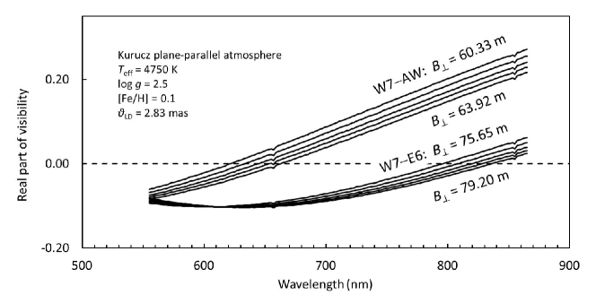
Figure 2: Modeled curves of ${\rm Re}[V(\lambda)]$ vs. $\lambda$ on two NPOI baselines for $\nu$ Ophiuchi based on a Kurucz model plane-parallel atmosphere with $T_{\rm eff}=4750$ K, $\log g=2.5$, and ${\rm[Fe/H]}=0.1$. We calculated ${\rm Re}(V)$ using a diameter $\theta_{\rm LD}=2.83$ mas and with projected baselines $B_{\perp}$ equal to those used in the 2005 June 29 observations shown in Fig. 1.

We applied the same procedure to spherical atmosphere models (Lester & Neilson, 2008; Neilson & Lester, 2008; Neilson, 2011) calculated by one of us (H. N.) for $T_{\rm eff}=4800$ K, $\log g=2.5$, ${\rm[Fe/H]}=0.1$, and mass $M=2.5M_{\odot}$. The mass, estimated as $2.6M_{\odot}$ by Allende Prieto & Lambert (1999), is a parameter in these models because it affects the depth of the atmosphere, an effect that is not important for plane-parallel models. The Neilson models are given with a wavelength resolution of 10 nm in the visual range and for 1000 values of $\mu$, so no interpolation in $\mu$ was needed. The resulting model curves are shown in Fig. 3. In this case, the input diameter that best fits the observations near 800 nm is 2.85 mas.

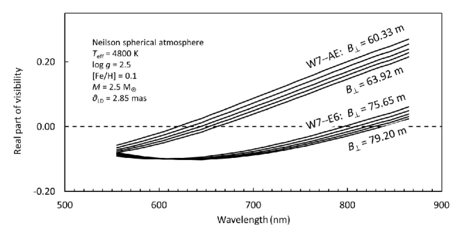
Figure 3: Modeled curves of ${\rm Re}[V(\lambda)]$ vs. $\lambda$ on two NPOI baselines for $\nu$ Ophiuchi based on a Neilson model spherical atmosphere with $T_{\rm eff}=4800$ K, $\log g=2.5$, $M=2.5M_{\odot}$ and ${\rm[Fe/H]}=0.1$. We calculated ${\rm Re}(V)$ using a diameter $\theta_{\rm LD}=2.85$ mas and with projected baselines $B_{\perp}$ equal to those used in the 2005 June 29 observations shown in Fig. 1.

5 Comparison with NPOI data

Figures 2 and 3 demonstrate that the zero-crossing wavelength $\lambda_{0}$ varies with the projected baseline length $B_{\perp}$. Whether $\theta_{\rm UD,0}$, derived from $\lambda_{0}$ and $B_{\perp}$, also varies depends on the brightness distribution. If the stellar disk were uniformly bright, $\theta_{\rm UD,0}$ would have a constant value, regardless of $\lambda_{0}$ and $B_{\perp}$.

Not surprisingly, our NPOI data from the G9 giant $\nu$ Ophiuchi demonstrate that the stellar disk is not uniformly bright. The dependence of $\theta_{\rm UD,0}$ on $\lambda_{0}$ is shown in Fig. 4. The two clusters of $\theta_{\rm UD,0}$ values correspond to data taken on two baselines. From a linear fit to the cluster around $\lambda 800$ nm (the solid line throught those data points in Fig. 4), the diameter with the smallest uncertainty, $\theta_{\rm UD,0}=2.6475\pm 0.0042$ mas, occurs at $\lambda_{0}=804$ nm. The two dashed lines bracketing those data show the envelope of best fit diameters $\pm 1\sigma$.

We have also plotted the predicted runs of $\theta_{\rm UD,0}(\lambda)$ for both a Kurucz and a Neilson model. In order to produce agreement with the data near 800 nm, we used limb-darkened diameters that differ by slightly less than 1% between the two models: 2.83 mas for the plane-parallel Kurucz model versus 2.85 mas for the spherical Neilson model. The difference may be related to the fact that emission from near the edge of the stellar disk is treated more realistically by a spherical model. In addition, the formal “edge” of the disk, where $\mu=1$ at some wavelength, does not represent how the variation of the depth of the atmosphere with wavelength affects which lines of sight reach an optical depth of unity as they graze the edge of the disk and which do not.

The curve showing the Kurucz model is actually multi-valued for a small region near the H$\alpha$ line: at projected baseline lengths near 65.13 m, decreased limb darkening near the H$\alpha$ line due to its higher opacity causes the equivalent uniform-disk diameter to increase. The Neilson model does not show this effect because it was calculated on a coarser wavelength grid. The slopes of the two models in Fig. 4 are slightly different; highly precise zero-crossing measurements would be needed to distinguish between them on this basis.

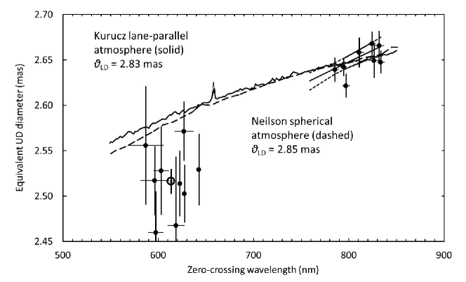
Figure 4: Equivalent uniform disk diameters $\theta_{\rm UD,0}(\lambda)$ (filled circles) derived from the spatial frequencies $u_{0}$ of the null in ${\rm Re}(V)$ in NPOI data and compared to representative Kurucz and Neilson atmosphere models. Vertical bars are $1\sigma$ errors. The solid line through the data near $\lambda 800$ nm shows a linear fit to that cluster of points, while the short-dashed curves above and below it show the $\theta_{\rm UD,0}\pm\sigma_{\theta}$ envelope around the linear fit. The open circle represents an average of the data in the shorter-wavelength cluster. Also shown are model $\theta_{\rm UD,0}(\lambda)$ curves for the Kurucz plane parallel (solid line) and Neilson spherical atmosphere (long-dashed line) models used to produce Figs. 2 and 3, with limb-darkened diameters chosen to match the NPOI data near $\lambda 800$ nm.

However, the most important feature of Fig. 4 is that the observed slope of $\theta_{\rm UD,0}(\lambda)$ differs significantly from both models, in the sense of requiring more limb darkening at shorter wavelengths. Although a detailed study of the atmosphere of $\nu$ Oph is beyond the scope of this paper, we explored the sensitivity of the slope of the Neilson model to its input parameters by calculating model $\theta_{\rm UD,0}(\lambda)$ curves for $T_{\rm eff}=4800$ K, $\log g=2.75$, $M=2.5M_{\odot}$ and ${\rm[Fe/H]}=0.0$ (i.e., slightly higher $\log g$ and lower metallicity than the model used in Fig. 4), and for $T_{\rm eff}=4900$ K, $\log g=2.50$, $M=2.5M_{\odot}$ and ${\rm[Fe/H]}=0.1$ (slightly higher $T_{\rm eff}$). The slopes are virtually identical. Lowering the metallicity and raising the surface gravity makes a tiny difference. Raising the temperature increases the model diameter by values ranging from $\approx 0.003$ mas at $\lambda$850 nm to $\approx 0.01$ mas at $\lambda$550 nm.

Mozurkewich et al. (2003) noted the same sense of disagreement between modeled and observed limb darkening in diameters measured with the Mark III interferometer, with $\theta_{\rm UD}(800~{}{\rm nm})/\theta_{\rm UD}(550~{}{\rm nm})$ being on average 0.8% larger than predicted in their results. The disagreement in our results for $\nu$ Oph are about the same magnitude.

6 Conclusion

Inspired by interferometric measurements of stellar angular diameters, we have presented a technique for measuring a closely related quantity, the uniform-disk diameter calculated from the spatial frequency at which we observe a null in the fringe visibility. This technique has the virtue of being free from multiplicative calibration uncertainties, unlike diameter measurements based on non-zero visibilities. As a result, the uncertainties in $\lambda_{0}$ are due to the number of photons and the spectral resolution with which they are gathered, and should decline approximately as $t^{1/2}$. Each of the scans used in the observations shown here were 30 s long due to instrumental limitations at the time of the observations, yet the precision with which they determine $\lambda_{0}$ is competitive with diameter determinations from nonzero fringe visibilities with only 1% calibration errors. In addition, our data were taken with relatively low spectral resolution, $\sim 50$. We expect that the combination of longer integration times and higher spectral resolution with, e.g., the VISION beam combiner at NPOI, will lead to significantly higher precision in measuring $\theta_{UD,0}$.

A second virtue of this technique is that we can use the combination of Earth rotation and spectrally resolved detection to explore how the null moves through spatial frequency space. In combination with higher spectral resolution, it will allow us to resolve the effects of such features as the H$\alpha$ signature apparent in the model curves in Figs. 2 and 4.

The comparison in §5 shows a distinct disagrement between the data and the atmosphere models in the sense that the data call for more limb darkening than the models produce. Our limited exploration of the sensitivity of the models to the input parameters shows that, for example, changing $T_{\rm eff}$ by 100 K is far from closing the gap. In future work, we intend to pursue this discrepancy further and to demonstrate the utility of this observational tool to probe stellar atmospheres.

References

- Absil et al. (2006) Absil, O., di Folco, E., Mérand, A., et al. 2006, Astron. Astrophys., 452, 237
- Allende Prieto & Lambert (1999) Allende Prieto, C., & Lambert, D. L. 1999, Astron. Astrophys., 352, 555
- Armstrong et al. (2012) Armstrong, J. T., Jorgensen, A. M., Neilson, H. R., et al. 2012, in Proc. SPIE, Vol. 8445, Optical and Infrared Interferometry III, ed. F. Delplancke, J. K. Rajagopal, & F. Malbet, 84453K
- Armstrong et al. (1998) Armstrong, J. T., Mozurkewich, D., Rickard, L. J., et al. 1998, Astrophys. J., 496, 550
- Baines et al. (2018) Baines, E. K., Armstrong, J. T., Schmitt, H. R., et al. 2018, Astron. J., 155, 30
- Ertel et al. (2014) Ertel, S., Absil, O., Defrère, D., et al. 2014, Astron. Astrophys., 570, 128
- Gallenne et al. (2018) Gallenne, A., Kervella, P., Evans, N. R., et al. 2018, Astrophys. J., 867, 121
- Garcia et al. (2016) Garcia, E. V., Muterspaugh, M. W., van Belle, G., et al. 2016, Pub. Astr. Soc. Pacific, 128, 055004 (21 p)
- Ghasempour et al. (2012) Ghasempour, A., Muterspaugh, M. W., Hutter, D. J., et al. 2012, in Proc. SPIE, Vol. 8445, Optical and Infrared Interferometry III, ed. F. Delplancke, J. K. Rajagopal, & F. Malbet, 84450M–84450M–8
- Gies et al. (2007) Gies, D. R., Jr., W. B., Baines, E. K., et al. 2007, Astrophys. J., 654, 527
- Jorgensen et al. (2010) Jorgensen, A. M., Schmitt, H., Armstrong, J. T., et al. 2010, in Proc. SPIE, Vol. 7734, Optical and Infrared Interferometry II, ed. W. C. Danchi, F. Delplancke, & J. K. Rajagopal, 77342Q–77342Q–13
- Kervella et al. (2006) Kervella, P., M’erand, A., Perrin, G., & Coudé du Foresto, V. 2006, Astron. Astrophys., 448, 623
- Lane et al. (2000) Lane, B. F., Kuchner, M. J., Boden, A. F., Creech-Eakman, M., & Kulkarni, S. R. 2000, Nature, 407, 485
- Lester & Neilson (2008) Lester, J. B., & Neilson, H. R. 2008, Astron. Astrophys., 491, 633
- Massarotti et al. (2007) Massarotti, A., Latham, D. W., Stefanik, R. P., & Fogel, J. 2007, Astron. J., 135, 209
- McWilliam (1990) McWilliam, A. 1990, Astrophys. J. Supp., 74, 1075
- Michelson (1891) Michelson, A. A. 1891, PASP, 3, 274
- Michelson & Pease (1921) Michelson, A. A., & Pease, F. G. 1921, Astrophys. J, 53, 249
- Mourard et al. (1989) Mourard, D., Bosc, I., Labeyrie, A., Koechlin, L., & Saha, S. 1989, Nature, 342, 520
- Mozurkewich et al. (2003) Mozurkewich, D., Armstrong, J. T., Hindsley, R. B., et al. 2003, Astron. J., 126, 2502
- Neilson (2011) Neilson, H. R. 2011, in Proc. IAU, Vol. 7, Interacting Binaries to Exoplanets: Essential Modeling Tools, 243–246
- Neilson & Lester (2008) Neilson, H. R., & Lester, J. B. 2008, Astron. Astrophys., 490, 807
- van Belle et al. (2018) van Belle, G. T., Armstrong, J. T., Benson, J. A., et al. 2018, in Proc. SPIE, Vol. 10701, Optical and Infrared Interferometry and Imaging VI, ed. M. Creech-Eakman, P. Tuthill, & A. Mérand, 1070105. https://doi.org/10.1117/12.2314204