$(BV,L^{p})$-decomposition, $p=1,2$, of functions in Metric Random Walk Spaces

Abstract.

In this paper we study the $(BV,L^{p})$-decomposition, $p=1,2$, of functions in metric random walk spaces, a general workspace that includes weighted graphs and nonlocal models used in image processing. We obtain the Euler-Lagrange equations of the corresponding variational problems and their gradient flows. In the case $p=1$ we also study the associated geometric problem and the thresholding parameters.

1. Introduction and Preliminaries

A metric random walk space $[X,d,m]$ is a metric space $(X,d)$ together with a family $m=(m_{x})_{x\in X}$ of probability measures that encode the jumps of a Markov chain. Important examples of metric random walk spaces are: locally finite weighted connected graphs, finite Markov chains and $[\mathbb{R}^{N},d,m^{J})$, with $d$ the Euclidean distance and

$$m^{J}_{x}(A):=\int_{A}J(x-y)d\mathcal{L}^{N}(y)\quad\hbox{for every Borel set }A\subset\mathbb{R}^{N},$$

where $J:\mathbb{R}^{N}\to[0,+\infty[$ is a measurable, nonnegative and radially symmetric function with mass equal to $1$. Furthermore, given a metric measure space $(X,d,\mu)$ we can obtain a metric random walk space $[X,d,m^{\mu,\epsilon}]$ called the $\epsilon$-step random walk associated to $\mu$, where

$$m^{\mu,\epsilon}_{x}:=\frac{\mu\!\!\mathop{\hbox{ \vrule height=7.0pt,width=0.5pt,depth=0.0pt\vrule height=0.5pt,width=6.0pt,depth=0.0pt}}\nolimits B(x,\epsilon)}{\mu(B(x,\epsilon))}.$$

Given a noisy image $f:\Omega\rightarrow\mathbb{R}$ on a rectangle $\Omega$ in $\mathbb{R}^{2}$, let us denote by $u:\Omega\rightarrow\mathbb{R}$ the desired cleaned image, which is related to the original one by

$$f=u+n,$$

when $n$ is an additive noise. The problem of recovering $u$ from $f$ is ill-posed (see [4]). To handle this problem, Rudin, Osher and Fatemi ([34]) proposed to solve the following constrained minimization problem

$$\begin{array}[]{ll}\hbox{Minimize}\ \displaystyle\int_{\Omega}|Du|\quad\hbox{with}\ \ \displaystyle\int_{\Omega}u=\int_{\Omega}f,\ \ \int_{\Omega}|u-f|^{2}=\sigma^{2}.\end{array}$$ (1.1)

The first constraint corresponds to the assumption that the noise has zero mean, and the second that its standard deviation is $\sigma$. Problem (1.1) is naturally linked to the following unconstrained problem (ROF-model):

$$\min\left\{\int_{\Omega}|Du|+\frac{\lambda}{2}\|u-f\|_{2}^{2}\ :\ u\in BV(\Omega)\right\},$$ (1.2)

for some Lagrange multiplier $\lambda>0$. Chambolle and Lions [12] proved an existence and uniqueness result for (1.1), as well as a proof of the link between (1.1) and (1.2). The constant $\lambda$ plays the role of a “scale parameter”. By tweaking $\lambda$, a user can select the level of detail desired in the reconstructed image.

The ROF-model leads to the $(BV,L^{2})$-decomposition of $f$:

$$f=u_{\lambda}+v_{\lambda},\quad[u_{\lambda},v_{\lambda}]=\displaystyle{\rm argmin}\left\{\int_{\Omega}|Du|+\frac{\lambda}{2}\|v\|_{2}^{2}\ :\ f=u+v\right\}.$$ (1.3)

This decomposition uses the $L^{2}$-fidelity term $\|f-u\|_{2}^{2}$. An alternative variational problem based on the $L^{1}$-fidelity term $\|f-u\|_{1}$ was proposed by Alliney ([1], [2]) in one dimensional spaces and was studied extensively by Chan, Esedoglu and Nikolova ([13], [14]):

$$f=u_{\lambda}+v_{\lambda},\quad[u_{\lambda},v_{\lambda}]=\displaystyle{\rm argmin}\left\{\int_{\Omega}|Du|+\lambda\|v\|_{1}\ :\ f=u+v\right\}.$$ (1.4)

The resulting $(BV,L^{1})$ minimization differs from the $(BV,L^{2})$ minimization in several important aspects which have attracted considerable attention in recent years (see [6], [16], [17], [21], [38] and the references therein). Let us point out that the $(BV,L^{1})$ minimization is contrast invariant (see [13]), as opposed to the $(BV,L^{2})$ minimization.

The use of neighborhood filters by Buades, Coll and Morel in [11], that was originally proposed by P. Yaroslavsky [37], has led to an extensive literature of nonlocal models in image processing (see for instance [8], [9], [21], [26], [27] and the references therein). This nonlocal ROF-model, in a simplified version, has the form

$$\min\left\{\int_{\Omega\times\Omega}J(x-y)|u(x)-u(y)|dxdy+\frac{\lambda}{2}\|u-f\|_{2}^{2}\ :\ u\in L^{2}(\Omega)\right\}.$$ (1.5)

On the other hand, an image can be seen as a weighted graph (see Example 1.1 (3)) where the pixels are taken as the vertices, and the weights are related to the similarity between pixels. Depending on the problem there are different ways to define the weights, see for instance [18], [24], [25] and [27]. The ROF-model in a weighted graph $G=(V(G),E(G),W(G))$ reads as follows:

$$\min\left\{\frac{1}{2}\sum_{x\in V(G)}\sum_{y\in V(G)}|u(y)-u(x)|w_{xy}+\frac{\lambda}{2}\sum_{x\in V(G)}|u(x)-f(x)|^{2}\sum_{y\sim x}w_{xy}:\ u\in L^{2}(G)\right\}.$$ (1.6)

Problems (1.5) and (1.6) are particular cases of the following ROF-model in a metric random walk space $[X,d,m]$ with invariant and reversible measure $\nu$:

$$\min\left\{\frac{1}{2}\int_{X}\int_{X}|u(y)-u(x)|dm_{x}(y)d\nu(x)+\frac{\lambda}{2}\int_{X}|u(x)-f(x)|^{2}d\nu(x):\ u\in L^{2}(X,\nu)\right\},$$ (1.7)

which is one of the motivations of this paper and we call $m$-ROF-model.

Another problem we are interested in is the $(BV,L^{1})$ minimization in a metric random walk space $[X,d,m]$, that reads as

$$\min\left\{\frac{1}{2}\int_{X}\int_{X}|u(y)-u(x)|dm_{x}(y)d\nu(x)+\lambda\int_{X}|u(x)-f(x)|d\nu(x):\ u\in L^{1}(X,\nu)\right\},$$ (1.8)

which has as a particular case the $(BV,L^{1})$ minimization in graphs.

The scale $\lambda$ in the $(BV,L^{2})$-decomposition (1.3) is viewed as a parameter that dictates the separation of the scale decomposition $f=u_{\lambda}+v_{\lambda}$. Following Meyer [32], $u_{\lambda}$ extracts the edges of $f$ while $v_{\lambda}$ captures textures.

In [34], to solve problem (1.1), the gradient descent method was used, which required to solve numerically the parabolic problem

$$\left\{\begin{array}[]{lll}u_{t}={\rm div}\left(\frac{Du}{|Du|}\right)-\lambda(u-f)&\hbox{in}\ (0,\infty)\times\Omega,\\ \\ \frac{Du}{|Du|}\eta=0&\hbox{on}\ (0,\infty)\times\partial\Omega,\\ \\ u(0,x)=v_{0}(x)&\hbox{in}\ x\in\Omega,\end{array}\right.$$ (1.9)

then the denoised version of $f$ is approached by the solution of (1.9) as $t$ increases. The concept of solution for which such problem is well-possed was given in [5]. We will see here that a non-local version of (1.9) can be used to approach the solutions of the ROF-problem in the workspace of metric random walk spaces (see Theorem 2.11).

Our aim is to study the $(BV,L^{p})$-decomposition, $p=1,2$, of functions in metric random walk spaces, developing a general theory that can be applied to weighted graphs and nonlocal models.

1.1. Metric Random Walk Spaces

Let $(X,d)$ be a Polish metric space equipped with its Borel $\sigma$-algebra. A random walk $m$ on $X$ is a family of probability measures $m_{x}$ on $X$, $x\in X$, satisfying the two technical conditions: (i) the measures $m_{x}$ depend measurably on the point $x\in X$, i.e., for any Borel set $A\subset X$ and any Borel set $B\subset\mathbb{R}$, the set $\{x\in X\ :\ m_{x}(A)\in B\}$ is Borel; (ii) each measure $m_{x}$ has finite first moment, i.e. for some (hence any) $z\in X$ and for any $x\in X$ one has $\int_{X}d(z,y)dm_{x}(y)<+\infty$ (see [33]).

A metric random walk space (or MRW space) $[X,d,m]$ is a Polish metric space $(X,d)$ together with a random walk $m$.

Let $[X,d,m]$ be a metric random walk space. A Radon measure $\nu$ on $X$ is invariant with respect to the random walk $m=(m_{x})$ if

$$d\nu(x)=\int_{y\in X}d\nu(y)dm_{y}(x),$$

that is, for any $\nu$-measurable set $A\subset X$, it holds that $A$ is $m_{x}$-measurable for $\nu$-almost all $x\in X$, $\displaystyle x\mapsto m_{x}(A)$ is $\nu$-measurable, and

$$\nu(A)=\int_{X}m_{x}(A)d\nu(x).$$

Consequently, if $\nu$ is an invariant measure with respect to $m$ and $f\in L^{1}(X,\nu)$, it holds that $f\in L^{1}(X,m_{x})$ for $\nu$-a.e. $x\in X$, $\displaystyle x\mapsto\int_{X}f(y)d{m_{x}}(y)$ is $\nu$-measurable, and

$$\int_{X}f(x)d\nu(x)=\int_{X}\left(\int_{X}f(y)d{m_{x}}(y)\right)d\nu(x).$$

The measure $\nu$ is said to be reversible for $m$ if moreover, the detailed balance condition

$$dm_{x}(y)d\nu(x)=dm_{y}(x)d\nu(y)$$

holds true. Under suitable assumptions on the metric random walk space $[X,d,m]$, such an invariant and reversible measure $\nu$ exists and is unique, as we will see below. Note that the reversibility condition implies the invariance condition.

We will assume that the metric measure space $(X,d)$ is $\sigma$-finite.

Example 1.1.

1. Consider $(\mathbb{R}^{N},d,\mathcal{L}^{N})$, with $d$ the Euclidean distance and $\mathcal{L}^{N}$ the Lebesgue measure. Let $J:\mathbb{R}^{N}\to[0,+\infty[$ be a measurable, nonnegative and radially symmetric function verifying $\int_{\mathbb{R}^{N}}J(z)dz=1$. In $(\mathbb{R}^{N},d,\mathcal{L}^{N})$ we have the following random walk, starting at $x$,

   $$m^{J}_{x}(A):=\int_{A}J(x-y)d\mathcal{L}^{N}(y)\quad\hbox{for every Borel set }A\subset\mathbb{R}^{N}.$$

   Applying Fubini’s Theorem it is easy to see that the Lebesgue measure $\mathcal{L}^{N}$ is an invariant and reversible measure for this random walk.

   In the case that $\Omega\subset\mathbb{R}^{N}$ is a closed bounded set, if, for $x\in\Omega$, we define

   $$m^{J,\Omega}_{x}(A):=\int_{A}J(x-y)dy+\left(\int_{\mathbb{R}^{n}\setminus\Omega}J(x-z)dz\right)\delta_{x}(A)\quad\forall A\subset\Omega\ \hbox{Borel},$$

   we have that each $m^{J,\Omega}_{x}$ is a probability measure in $\Omega$. Moreover, it is easy to see ([30]) that $\nu=\mathcal{L}^{N}\!\!\mathop{\hbox{ \vrule height=7.0pt,width=0.5pt,depth=0.0pt\vrule height=0.5pt,width=6.0pt,depth=0.0pt}}\nolimits\Omega$ is an invariant and reversible measure for the random walk $m^{J,\Omega}=(m^{J,\Omega}_{x})_{x\in\Omega}$.

2. Let $K:X\times X\rightarrow\mathbb{R}$ be a Markov kernel on a countable space $X$, i.e.,

   $$K(x,y)\geq 0,\quad\forall x,y\in X,\quad\quad\sum_{y\in X}K(x,y)=1\quad\forall x\in X.$$

   Then, for

   $$m^{K}_{x}(A):=\sum_{y\in A}K(x,y),$$

   $[X,d,m^{K}]$ is a metric random walk space for any metric $d$ on $X$. Basic Markov chain theory guarantees the existence of a unique stationary probability measure (also called steady state) $\pi$ on $X$, that is,

   $$\sum_{x\in X}\pi(x)=1\quad\hbox{and}\quad\pi(y)=\sum_{x\in X}\pi(x)K(x,y)\quad\quad\forall y\in X.$$

   We say that $\pi$ is reversible for $K$ if the following detailed balance equation

   $$K(x,y)\pi(x)=K(y,x)\pi(y)$$

   holds true for $x,y\in X$.

3. Consider a locally finite weighted discrete graph $G=(V(G),E(G))$, where each edge $(x,y)\in E(G)$ (we will write $x\sim y$ if $(x,y)\in E(G)$) has a positive weight $w_{xy}=w_{yx}$ assigned. Suppose further that $w_{xy}=0$ if $(x,y)\not\in E(G)$. The graph is equipped with the standard shortest path graph distance $d_{G}$, that is, $d_{G}(x,y)$ is the minimal number of edges connecting $x$ and $y$. We will assume that any two points are connected, i.e., that the graph is connected. For $x\in V(G)$ we define the weight at the vertex $x$ as

   $$d_{x}:=\sum_{y\sim x}w_{xy}=\sum_{y\in V(G)}w_{xy},$$

   and the neighbourhood $N_{G}(x):=\{y\in V(G)\ :\ x\sim y\}$. By definition of locally finite graph, the sets $N_{G}(x)$ are finite. When $w_{x,y}=1$ for every $x,y\in V(G)$, $d_{x}$ coincides with the degree of the vertex $x$ in the graph, that is, the number of edges containing vertex $x$.

   For each $x\in V(G)$ we define the following probability measure

   $$m^{G}_{x}=\frac{1}{d_{x}}\sum_{y\sim x}w_{xy}\,\delta_{y}.\\ \\$$ (1.10)

   We have that $[V(G),d_{G},(m^{G}_{x})]$ is a metric random walk space. It is not difficult to see that the measure $\nu_{G}$ defined as

   $$\nu_{G}(A):=\sum_{x\in A}d_{x},\quad A\subset V(G),$$

   is an invariant and reversible measure for this random walk.

   Given a locally finite weighted discrete graph $G=(V(G),E(G))$, there is a natural definition of a Markov chain on the vertices. We define the Markov kernell $K_{G}:V(G)\times V(G)\rightarrow\mathbb{R}$ as

   $$K_{G}(x,y):=\frac{1}{d_{x}}w_{xy}.$$

   We have that $m^{G}$ and $m^{K_{G}}$ define the same random walk. If $\nu_{G}(V(G))$ is finite, the unique stationary and reversible probability measure is given by

   $$\pi_{G}(\{x\}):=\frac{1}{\nu_{G}(V(G))}\sum_{z\in V(G)}w_{xz}.$$

   In Machine Learning Theory ([19], [20]) an example of a weighted discrete graph is a point cloud in $\mathbb{R}^{N}$, $V=\{x_{1},\ldots,x_{n}\}$, with edge weights $w_{x_{i},x_{j}}$ given by

   $$w_{x_{i},x_{j}}:=\eta(|x_{i}-x_{j}|),\quad 1\leq i,j\leq n,$$

   where the kernel $\eta:[0,\infty)\rightarrow[0,\infty)$ is a radial profile satisfying

   • $\eta(0)>0$, and $\eta$ is continuous at $0$,

   • $\eta$ is non-decreasing,

   • and the integral $\int_{0}^{\infty}\eta(r)r^{N}dr$ is finite.

4. From a metric measure space $(X,d,\mu)$ we can obtain a metric random walk space, the so called $\epsilon$-step random walk associated to $\mu$, as follows. Assume that balls in $X$ have finite measure and that ${\rm Supp}(\mu)=X$. Given $\epsilon>0$, the $\epsilon$-step random walk on $X$, starting at point $x$, consists in randomly jumping in the ball of radius $\epsilon$ around $x$, with probability proportional to $\mu$; namely

   $$m^{\mu,\epsilon}_{x}:=\frac{\mu\!\!\mathop{\hbox{ \vrule height=7.0pt,width=0.5pt,depth=0.0pt\vrule height=0.5pt,width=6.0pt,depth=0.0pt}}\nolimits B(x,\epsilon)}{\mu(B(x,\epsilon))}.$$

   Note that $\mu$ is an invariant and reversible measure for the metric random walk space $[X,d,m^{\mu,\epsilon}]$.

5. Given a metric random walk space $[X,d,m]$ with invariant and reversible measure $\nu$, and given a $\nu$-measurable set $\Omega\subset X$ with $\nu(\Omega)>0$, if we define, for $x\in\Omega$,

   $$m^{\Omega}_{x}(A):=\int_{A}dm_{x}(y)+\left(\int_{X\setminus\Omega}dm_{x}(y)\right)\delta_{x}(A)\quad\hbox{ for every Borel set }A\subset\Omega,$$

   we have that $[\Omega,d,m^{\Omega}]$ is a metric random walk space and it easy to see that $\nu\!\!\mathop{\hbox{ \vrule height=7.0pt,width=0.5pt,depth=0.0pt\vrule height=0.5pt,width=6.0pt,depth=0.0pt}}\nolimits\Omega$ is reversible for $m^{\Omega}$.

From now on we will assume that $[X,d,m]$ is a metric random walk space with a reversible measure $\nu$ for $m$.

1.2. $m$-Perimeter

We introduce the $m$-interaction between two $\nu$-measurable subsets $A$ and $B$ of $X$ as

$$L_{m}(A,B):=\int_{A}\int_{B}dm_{x}(y)d\nu(x).$$ (1.11)

Whenever $L_{m}(A,B)<\infty$, by the reversibility assumption on $\nu$ with respect to $m$, we have

$$L_{m}(A,B)=L_{m}(B,A).$$

We define the concept of $m$-perimeter of a $\nu$-measurable subset $E\subset X$ as

$$P_{m}(E)=L_{m}(E,X\setminus E)=\int_{E}\int_{X\setminus E}dm_{x}(y)d\nu(x).$$

It is easy to see that

$$P_{m}(E)=\frac{1}{2}\int_{X}\int_{X}|\raisebox{2.0pt}{\rm{$\chi$}}_{E}(y)-\raisebox{2.0pt}{\rm{$\chi$}}_{E}(x)|dm_{x}(y)d\nu(x).$$ (1.12)

Moreover, if $\nu(E)<+\infty$, we have

$$P_{m}(E)=\nu(E)-\int_{E}\int_{E}dm_{x}(y)d\nu(x).$$ (1.13)

Example 1.2.

1. Let $[\mathbb{R}^{N},d,m^{J}]$ be the metric random walk space given in Example 1.1 (1) with invariant measure $\mathcal{L}^{N}$. Then,

   $$P_{m^{J}}(E)=\frac{1}{2}\int_{\mathbb{R}^{N}}\int_{\mathbb{R}^{N}}|\raisebox{2.0pt}{\rm{$\chi$}}_{E}(y)-\raisebox{2.0pt}{\rm{$\chi$}}_{E}(x)|J(x-y)dydx,$$

   which coincides with the concept of $J$-perimeter introduced in [28] (see also [29]). On the other hand,

   $$P_{m^{J,\Omega}}(E)=\frac{1}{2}\int_{\Omega}\int_{\Omega}|\raisebox{2.0pt}{\rm{$\chi$}}_{E}(y)-\raisebox{2.0pt}{\rm{$\chi$}}_{E}(x)|J(x-y)dydx.$$

   Note that, in general, $P_{m^{J,\Omega}}(E)\not=P_{m^{J}}(E).$

2. In the case of the metric random walk space $[V(G),d_{G},m^{G}]$ associated to a finite weighted discrete graph $G$, given $A,B\subset V(G)$, ${\rm Cut}(A,B)$ is defined as

   $${\rm Cut}(A,B):=\sum_{x\in A,y\in B}w_{xy}=L_{m^{G}}(A,B),$$

   and the perimeter of a set $E\subset V(G)$ is given by

   $$|\partial E|:={\rm Cut}(E,E^{c})=\sum_{x\in E,y\in V\setminus E}w_{xy}.$$

   Consequently, we have that

   $$|\partial E|=P_{m^{G}}(E)\quad\hbox{for all}\ E\subset V(G).$$ (1.14)

Let us now remember some properties of the $m$-perimeter given in [31].

Proposition 1.3 ([31]).

1. Let $A,\ B\subset X$ be $\nu$-measurable sets with finite $m$-perimeter such that $\nu(A\cap B)=0$. Then,

$$P_{m}(A\cup B)=P_{m}(A)+P_{m}(B)-2L_{m}(A,B).$$

2. Let $A,\ B,\ C$ be $\nu$-measurable sets in $X$ with pairwise $\nu$-null intersections. Then

$$P_{m}(A\cup B\cup C)=P_{m}(A\cup B)+P_{m}(A\cup C)+P_{m}(B\cup C)-P_{m}(A)-P_{m}(B)-P_{m}(C).$$

Proposition 1.4 (Submodularity).

Let $A$ and $B$ be $\nu$-measurable sets in $X$. Then

$$P_{m}(A\cup B)+P_{m}(A\cap B)=P_{m}(A)+P_{m}(B)-2L_{m}(A\setminus B,B\setminus A).$$

Consequently,

$$P_{m}(A\cup B)+P_{m}(A\cap B)\leq P_{m}(A)+P_{m}(B).$$

Proof.

By Proposition 1.3 2,

$$\begin{array}[]{l}\displaystyle P_{m}(A\cup B)=P_{m}\big{(}(A\setminus B)\cup(B\setminus A)\cup(A\cap B)\big{)}\\ \\ \displaystyle\phantom{P_{m}(A\cup B)}=P_{m}\big{(}(A\setminus B)\cup(B\setminus A)\big{)}+P_{m}(A)+P_{m}(B)\\ \\ \displaystyle\phantom{P_{m}(A\cup B)=}-P_{m}(A\setminus B)-P_{m}(B\setminus A)-P_{m}(A\cap B).\end{array}$$

Hence,

$$\begin{array}[]{l}\displaystyle P_{m}(A\cup B)+P_{m}(A\cap B)=P_{m}(A)+P_{m}(B)\\ \\ \displaystyle\phantom{P_{m}(A\cup B)+P_{m}(A\cap B)=}+P_{m}\big{(}(A\setminus B)\cup(B\setminus A)\big{)}-P_{m}(A\setminus B)-P_{m}(B\setminus A).\end{array}$$

Now, by Proposition 1.3 1.,

$$P_{m}\big{(}(A\setminus B)\cup(B\setminus A)\big{)}-P_{m}(A\setminus B)-P_{m}(B\setminus A)=-2L_{m}(A\setminus B,B\setminus A).$$

$\Box$

1.3. $m$-Total Variation

Associated with the random walk $m=(m_{x})$ and the invariant measure $\nu$, we define the space

$$BV_{m}(X):=\left\{u:X\to\mathbb{R}\ \hbox{ $\nu$-measurable}\,:\,\int_{X}\int_{X}|u(y)-u(x)|dm_{x}(y)d\nu(x)<\infty\right\}.$$

We have that $L^{1}(X,\nu)\subset BV_{m}(X)$. The $m$-total variation of a function $u\in BV_{m}(X)$ is defined by

$$TV_{m}(u):=\frac{1}{2}\int_{X}\int_{X}|u(y)-u(x)|dm_{x}(y)d\nu(x).$$

Note that

$$P_{m}(E)=TV_{m}(\raisebox{2.0pt}{\rm{$\chi$}}_{E}).$$

Recall the definition of the generalized product measure $\nu\otimes m_{x}$ (see, for instance, [3]), which is defined as the measure in $X\times X$ given by

$$\nu\otimes m_{x}(U):=\int_{X}\int_{X}\raisebox{2.0pt}{\rm{$\chi$}}_{U}(x,y)dm_{x}(y)d\nu(x)\quad\hbox{for }U\in\mathcal{B}(X\times X),$$

where one needs the map $x\mapsto m_{x}(E)$ to be $\nu$-measurable for any Borel set $E\in\mathcal{B}(X)$. It holds that

$$\int_{X\times X}gd(\nu\otimes m_{x})=\int_{X}\int_{X}g(x,y)dm_{x}(y)d\nu(x)$$

for every $g\in L^{1}(X\times X,\nu\otimes m_{x})$. Therefore, we can write

$$TV_{m}(u)=\frac{1}{2}\int_{X}\int_{X}|u(y)-u(x)|d(\nu\otimes m_{x})(x,y).$$

Example 1.5.

Let $[V(G),d_{G},(m^{G}_{x})]$ be the metric random walk space given in Example 1.1 (3) with invariant measure $\nu_{G}$. Then

$$TV_{m^{G}}(u)=\frac{1}{2}\int_{V(G)}\int_{V(G)}|u(y)-u(x)|dm^{G}_{x}(y)d\nu_{G}(x)$$

$$=\frac{1}{2}\int_{V(G)}\frac{1}{d_{x}}\left(\sum_{y\in V(G)}|u(y)-u(x)|w_{xy}\right)d\nu_{G}(x)$$

$$=\frac{1}{2}\sum_{x\in V(G)}d_{x}\left(\frac{1}{d_{x}}\sum_{y\in V(G)}|u(y)-u(x)|w_{xy}\right)=\frac{1}{2}\sum_{x\in V(G)}\sum_{y\in V(G)}|u(y)-u(x)|w_{xy}.$$

Note that $TV_{m^{G}}(u)$ coincides with the anisotropic total variation $TV^{1}_{a}(u)$ defined in [22].

The next results are proved in [31].

Lemma 1.6 ([31]).

$TV_{m}$ is lower semi-continuous with respect to the the weak convergence in $L^{2}(X,\nu)$.

Theorem 1.7 (Coarea formula, [31]).

For any $u\in L^{1}(X,\nu)$, let $E_{t}(u):=\{x\in X\,:\,u(x)>t\}$. Then,

$$TV_{m}(u)=\int_{-\infty}^{+\infty}P_{m}(E_{t}(u))\,dt.$$ (1.15)

1.4. The $1$-Laplacian in MRW Spaces

Given a function $u:X\rightarrow\mathbb{R}$ we define its nonlocal gradient $\nabla u:X\times X\rightarrow\mathbb{R}$ as

$$\nabla u(x,y):=u(y)-u(x)\quad\forall\,x,y\in X.$$

For a function ${\bf z}:X\times X\rightarrow\mathbb{R}$, its $m$-divergence ${\rm div}_{m}{\bf z}:X\rightarrow\mathbb{R}$ is defined as

$$({\rm div}_{m}{\bf z})(x):=\frac{1}{2}\int_{X}({\bf z}(x,y)-{\bf z}(y,x))dm_{x}(y).$$

For $p\geq 1$, we define the space

$$X_{m}^{p}(X):=\left\{{\bf z}\in L^{\infty}(X\times X,\nu\otimes m_{x})\ :\ {\rm div}_{m}{\bf z}\in L^{p}(X,\nu)\right\}.$$

Let $u\in BV_{m}(X)\cap L^{p^{\prime}}(X,\nu)$ and ${\bf z}\in X_{m}^{p}(X)$, $1\leq p\leq\infty$, having in mind that $\nu$ is reversible, we have the following Green’s formula

$$\int_{X}u(x)({\rm div}_{m}{\bf z})(x)dx=-\frac{1}{2}\int_{X\times X}\nabla u(x,y){\bf z}(x,y)d\nu\otimes dm_{x}.$$ (1.16)

Let us denote by $\hbox{sign}(r)$ the multivalued sign function

$${\rm sign}(u)(x):=\left\{\begin{array}[]{lll}1&\hbox{if}\ \ u(x)>0,\\ -1&\hbox{if}\ \ u(x)<0,\\ \left[-1,1\right]&\hbox{if}\ \ \ u(x)=0.\end{array}\right.$$

The functional $\mathcal{F}_{m}:L^{2}(X,\nu)\rightarrow]-\infty,+\infty]$ defined by

$$\mathcal{F}_{m}(u):=\left\{\begin{array}[]{ll}\displaystyle TV_{m}(u)&\hbox{if}\ u\in L^{2}(X,\nu)\cap BV_{m}(X),\\[10.0pt] +\infty&\hbox{if }u\in L^{2}(X,\nu)\setminus BV_{m}(X),\end{array}\right.$$

is convex and lower semi-continuous. The following characterizations for its subdifferential have been proved in [31].

Theorem 1.8 ([31]).

Let $u\in L^{2}(X,\nu)$ and $v\in L^{2}(X,\nu)$. The following assertions are equivalent:

$v\in\partial\mathcal{F}_{m}(u)$;

there exists ${\bf z}\in X_{m}^{2}(X)$, $\|{\bf z}\|_{\infty}\leq 1$ such that

$$v=-{\rm div}_{m}{\bf z}$$ (1.17)

and

$$\int_{X}u(x)v(x)d\nu(x)=\mathcal{F}_{m}(u);$$ (1.18)

there exists ${\bf z}\in X_{m}^{2}(X)$, $\|{\bf z}\|_{\infty}\leq 1$ such that (1.17) holds and

$$\mathcal{F}_{m}(u)=\frac{1}{2}\int_{X\times X}\nabla u(x,y){\bf z}(x,y)d\nu\otimes dm_{x};$$ (1.19)

there exists $\hbox{\bf g}\in L^{\infty}(X\times X,\nu\otimes m_{x})$ antisymmetric with $\|\hbox{\bf g}\|_{\infty}\leq 1$ such that

$$-\int_{X}{\bf g}(x,y)\,dm_{x}(y)=v(x)\quad\nu-\mbox{a.e }x\in X,$$ (1.20)

and

$$-\int_{X}\int_{X}\hbox{\bf g}(x,y)dm_{x}(y)\,u(x)d\nu(x)=\mathcal{F}_{m}(u).$$ (1.21)

there exists $\hbox{\bf g}\in L^{\infty}(X\times X,\nu\otimes m_{x})$ antisymmetric with $\|\hbox{\bf g}\|_{\infty}\leq 1$ verifying (1.20) and

$$\hbox{\bf g}(x,y)\in{\rm sign}(u(y)-u(x))\quad(\nu\otimes m_{x})-a.e.\ (x,y)\in X\times X.$$ (1.22)

Remark 1.9.

The next space was introduced in [32] in the continuous setting. Set

$$G_{m}(X):=\{f\in L^{2}(X,\nu)\ :\ \exists{\bf z}\in X^{2}_{m}(X)\ \hbox{such that}\ f={\rm div}_{m}({\bf z})\}$$

and consider in $G_{m}(X)$ the norm

$$\|f\|_{m,*}:=\inf\{\|{\bf z}\|_{\infty}\ :\ f={\rm div}_{m}({\bf z})\}.$$

From the proof of [31, Theorem 3.3] we have that

$$\|f\|_{m,*}=\sup\left\{\left|\int_{X}f(x)u(x)d\nu(x)\right|\ :u\in L^{2}(X,\nu),\ TV_{m}(u)\leq 1\right\},$$ (1.23)

and

$$\partial\mathcal{F}_{m}(u)=\left\{v\in G_{m}(X)\,:\,\|v\|_{m,*}\leq 1,\ \ \int_{X}u(x)v(x)d\nu(x)=\mathcal{F}_{m}(u)\right\}.$$ (1.24)

In particular,

$$\partial\mathcal{F}_{m}(0)=\{v\in G_{m}(X)\,:\,\|v\|_{m,*}\leq 1\}.$$ (1.25)

Definition 1.10.

We define the multivalued operator $\Delta^{m}_{1}$ in $L^{2}(X,\nu)$ by $(u,v)\in\Delta^{m}_{1}$ if, and only if, $-v\in\partial\mathcal{F}_{m}(u)$.

It is easy to see that $-\Delta^{m}_{1}$ is a completely accretive operator (see [7]).

Chang, in [15], and Hein and Bühler, in [23], define a similar operator in the particular case of finite graphs.

We finish this section by recalling some concepts studied in [31] that will be used later.

Definition 1.11.

A pair $(\lambda,u)\in\mathbb{R}\times L^{2}(X,\nu)$ is called an $m$-eigenpair of the $1$-Laplacian $\Delta^{m}_{1}$ on $X$ if $\|u\|_{1}=1$ and there exists $\xi\in{\rm sign}(u)$ such that

$$\lambda\,\xi\in-\Delta^{m}_{1}u.$$ (1.26)

The constant $\lambda$ is called $m$-eigenvalue and the function $u$ is an $m$-eigenfunction associated to $\lambda$.

Given a function $u:X\rightarrow\mathbb{R}$, $\mu\in\mathbb{R}$ is a median of $u$ with respect to the measure $\nu$ if

$$\nu(\{x\in X\ :\ u(x)<\mu\})\leq\frac{1}{2}\nu(X),\quad\nu(\{x\in X\ :\ u(x)>\mu\})\leq\frac{1}{2}\nu(X).$$

We denote by ${\rm med}_{\nu}(u)$ the set of all medians of $u$. It is easy to see that

$${\rm argmin}\left\{\int_{X}|f-c|\ :\ c\in\mathbb{R}\right\}={\rm med}_{\nu}(f)$$ (1.27)

and

$$0\in{\rm med}_{\nu}(u)\iff\exists\xi\in{\rm sign}(u)\ \hbox{such that}\ \int_{X}\xi(x)d\nu(x)=0.$$ (1.28)

Given a set $\Omega\subset X$ with $0<\nu(\Omega)<\nu(X)$, we denote

$$\lambda^{m}_{\Omega}:=\frac{P_{m}(\Omega)}{\nu(\Omega)},$$

and we define the $m$-Cheeger constant of $\Omega$ by

$$h_{1}^{m}(\Omega):=\inf\left\{\lambda^{m}_{E}\,:\,E\subset\Omega,\ E\ \hbox{$\nu$-measurable and }\,\nu(E)>0\right\}.$$ (1.29)

A $\nu$-measurable set $E\subset\Omega$ achieving the infimum in (1.29) is said to be an $m$-Cheeger set of $\Omega$. Furthermore, we say that $\Omega$ is $m$-calibrable if it is an $m$-Cheeger set of itself, that is, if $h_{1}^{m}(\Omega)=\lambda^{m}_{\Omega}.$

Definition 1.12.

A Borel set $B\subset X$ is said to be invariant with respect to the random walk $m$ if $m_{x}(B)=1$ whenever $x\in B$. An invariant probability measure $\nu$ is said to be ergodic with respect to $m$ if $\nu(B)=0$ or $\nu(B)=1$ for every invariant set $B$ with respect to the random walk $m$.

If $\nu$ is ergodic with respect to $m$ then (see [31])

$$TV_{m}(u)=0\iff u\ \hbox{is $\nu$-a.e. equal to a constant}.$$

From now on we will assume that $\nu$ is finite and that $\frac{1}{\nu(X)}\nu$ is ergodic with respect to $m$. See [31] for characterizations of the ergodicity.

2. The Rudin-Osher-Fatemi Model in MRW Spaces

2.1. The $m$-ROF Model

We consider the following ROF-problem

$$\min\left\{TV_{m}(u)+\frac{\lambda}{2}\int_{X}|u(x)-f(x)|^{2}d\nu(x):\ u\in L^{2}(X,\nu)\right\},$$ (2.1)

for $f\in L^{2}(X,\nu)$ and $\lambda>0$. We start by proving existence and uniqueness of the minimizer for problem (2.1) and a characterization.

Let us write

$$\mathcal{G}_{m}(u,f,\lambda):=TV_{m}(u)+\frac{\lambda}{2}\|u-f\|^{2}_{L^{2}(X,\nu)}.$$

Theorem 2.1.

For any $f\in L^{2}(X,\nu)$ and $\lambda>0$, there exists a unique minimizer $u_{\lambda}$ of problem (2.1). Moreover, $u_{\lambda}$ is the unique solution of the problem

$$\lambda(u-f)\in\Delta_{1}^{m}(u).$$ (2.2)

Consequently, $u_{\lambda}\in L^{2}(X,\nu)$ is the solution of problem (2.1) if, and only if, there exists $\hbox{\bf g}\in L^{\infty}(X\times X,\nu\otimes m_{x})$ antisymmetric with $\|\hbox{\bf g}\|_{\infty}\leq 1$, such that

$$\lambda(u_{\lambda}-f)={\rm div}_{m}{\bf g}$$ (2.3)

and

$${\bf g}(x,y)\in{\rm sign}(u_{\lambda}(y)-u_{\lambda}(x))\quad(\nu\otimes m_{x})-a.e.\ (x,y)\in X\times X.$$

Proof.

Let $\{u_{n}\}_{n\in N}$ be a minimizing sequence of problem (2.1). Then,

$$\alpha:=\inf\left\{\mathcal{G}_{m}(u,f,\lambda)\ :\ u\in L^{2}(X,\nu)\right\}=\lim_{n\to\infty}\mathcal{G}_{m}(u_{n},f,\lambda).$$

Since

$$\|u_{n}\|^{2}_{L^{2}(X,\nu)}\leq 2\left(\|u_{n}-f\|^{2}_{L^{2}(X,\nu)}+\|f\|^{2}_{L^{2}(X,\nu)}\right)\leq 2\left(\frac{2}{\lambda}\mathcal{G}_{m}(u_{n},f,\lambda)+\|f\|^{2}_{L^{2}(X,\nu)}\right),$$

we have that $\{u_{n}\}_{n}$ is bounded in $L^{2}(X,\nu)$, and we can assume that, up to a subsequence,

$$u_{n}\to u_{\lambda}\quad\hbox{weakly in}\ L^{2}(X,\nu).$$

Therefore, by the lower semi-continuity of the $L^{2}$-norm with respect to the weak convergence and Lemma 1.6, we have that

$$\mathcal{G}_{m}(u_{\lambda},f,\lambda)\leq\liminf_{n\to\infty}\mathcal{G}_{m}(u_{n},f,\lambda)=\alpha,$$

and, consequently, $u_{\lambda}$ is a minimizer of problem (2.1). Uniqueness follows from the strict convexity of $\|\cdot\|_{L^{2}(X,\nu)}^{2}$ and the convexity of $TV_{m}$.

Since $u_{\lambda}$ is a minimizer of problem (2.1), we have that $0\in\partial\mathcal{G}_{m}(u_{\lambda},f,\lambda)$. Now, if $\Phi(u):=\frac{\lambda}{2}\|u-f\|^{2}_{L^{2}(X,\nu)}$, then, by [10, Corollary 2.11], we have that

$$\partial\mathcal{G}_{m}(u,f,\lambda)=\partial\mathcal{F}_{m}(u)+\partial\Phi(u),$$

thus

$$0\in\partial\mathcal{G}_{m}(u_{\lambda},f,\lambda)=\partial\mathcal{F}_{m}(u_{\lambda})+\lambda(u_{\lambda}-f),$$

which gives (2.2). Then, the characterization of $u_{\lambda}$ follows from Theorem 1.8. $\Box$

Observe that, on account of (1.24), we have that $u_{\lambda}$ is the solution of problem (2.1) if, and only if,

$$\left\{\begin{array}[]{l}\displaystyle f-u_{\lambda}\in G_{m}(X),\\[8.0pt] \|f-u_{\lambda}\|_{m^{*}}\leq\frac{1}{\lambda}\ \hbox{ and}\\[8.0pt] \displaystyle\lambda\int_{X}(f-u_{\lambda})u_{\lambda}d\nu=TV_{m}(u_{\lambda}).\end{array}\right.$$ (2.4)

As a consequence of this we have:

Proposition 2.2.

Let $f\in L^{2}(X,\nu)$ and $\lambda>0$. Then, $u_{\lambda}=0$ is the solution of problem (2.1) if, and only if,

$$f\in G_{m}(X)\quad\hbox{and}\quad\|f\|_{m,*}\leq\frac{1}{\lambda}.$$

For $f\in G_{m}(X)$, if $\|f\|_{m,*}>\frac{1}{\lambda}$ then $u_{\lambda}$ is characterized by the following two conditions

$$\|f-u_{\lambda}\|_{m,*}=\frac{1}{\lambda}$$ (2.5)

and

$$\lambda\int_{X}(f-u_{\lambda})u_{\lambda}d\nu=TV_{m}(u_{\lambda}).$$ (2.6)

Proof.

The first part follows from (2.4). Let $f\in G_{m}(X)$ with $\|f\|_{m,*}>\frac{1}{\lambda}$. From (2.4) again,

$$\|\lambda(f-u_{\lambda})\|_{m,*}\leq 1\quad\hbox{and}\quad\lambda\int_{X}(f-u_{\lambda})u_{\lambda}d\nu=TV_{m}(u_{\lambda}).$$

Now, since $\|f\|_{m,*}>\frac{1}{\lambda}$, we know that $u_{\lambda}\not\equiv 0$, thus, by (1.23), we have

$$\|\lambda(f-u_{\lambda})\|_{m,*}\geq\frac{\lambda}{TV_{m}(u_{\lambda})}\int_{X}(f-u_{\lambda})u_{\lambda}d\nu=1.$$

Therefore,

$$\|f-u_{\lambda}\|_{m,*}=\frac{1}{\lambda},$$

and we conclude the proof. $\Box$

The $m$-ROF-model leads to the $(BV,L^{2})$-decomposition

$$f=u_{\lambda}+v_{\lambda}\ ,\quad[u_{\lambda},v_{\lambda}]=\displaystyle{\rm argmin}\left\{TV_{m}(u)+\frac{\lambda}{2}\|v\|_{2}^{2}\ :\ f=u+v\right\}.$$ (2.7)

Then, from the previous results, we can rewrite:

Corollary 2.3.

Let $f\in L^{2}(X,\nu)$ and $\lambda>0$. For the $(BV,L^{2})$-decomposition $[u_{\lambda},v_{\lambda}]$ of $f$, we have:

$v_{\lambda}\in G_{m}(X)$, $\|v_{\lambda}\|_{m^{*}}\leq\frac{1}{\lambda}$  and  $\displaystyle\lambda\int_{X}v_{\lambda}u_{\lambda}d\nu=TV_{m}(u_{\lambda})$.

$u_{\lambda}=0$ if, and only if, $v_{\lambda}=f$.

For $f\in G_{m}(X)$, if $\|f\|_{m,*}>\frac{1}{\lambda}$ then

$$\|v_{\lambda}\|_{m,*}=\frac{1}{\lambda}\quad\hbox{and}\quad\lambda\int_{X}v_{\lambda}u_{\lambda}d\nu=TV_{m}(u_{\lambda}).$$

Remark 2.4.

(i) If $\lambda$ is too small then the regularization term $TV_{m}(u)$ is excessively penalized and the image is over-smoothed, resulting in a loss of information in the reconstructed image. On the other hand, if $\lambda$ is too large then the reconstructed image is under-regularized and noise is left in the reconstruction.

In [35] and [36], Tadmor, Nezzar and Vese propose a multiscale decomposition in order to overcome the difficulties observed in the previous point. In this regard, the space of functions $G_{m}(X)$ is of particular interest, since, as we have seen in Corollary 2.7, after a first decomposition $[u_{\lambda},v_{\lambda}]$ the function $v_{\lambda}$ is a function of $G_{m}(X)$ which in turn can be decomposed. The multiscale decomposition takes advantage of this fact by taking an increasing sequence of scales $\lambda_{i}$ tending to infinity and inductively applying the $(BV,L^{2})$-decomposition with scale parameter $\lambda_{i+1}$ to $v_{\lambda_{i}}$ so that after $k$-steps we have

$$f=\sum_{i=1}^{k}u_{\lambda_{i}}+v_{\lambda_{k}},\quad\|v_{\lambda_{k}}\|_{m^{*}}\leq\frac{1}{\lambda_{k}}.$$

Integrating both sides of (2.3) over $X$ and using Green’s formula (1.16), with $u=1$ and ${\bf z}={\bf g}$, on the right-hand side we get:

Proposition 2.5.

If $u_{\lambda}$ is the unique minimizer of problem (2.1) with noisy image $f$ then

$$\int_{X}u_{\lambda}(x)d\nu(x)=\int_{X}f(x)d\nu(x).$$

Furthermore, we have the following Maximum Principle.

Proposition 2.6.

If $[u_{i,\lambda},v_{i,\lambda}]$ is the $(BV,L^{2})$-decomposition of $f_{i}$, $i=1,2$, then

$$\|(u_{1,\lambda}-u_{2,\lambda})^{+}\|_{2}\leq\|(f_{1}-f_{2})^{+}\|_{2}.$$ (2.8)

In particular, for $c,\,C\in\mathbb{R}$, if $c\leq f\leq C$ $\nu$-a.e., and $[u_{\lambda},v_{\lambda}]$ is the $(BV,L^{2})$-decomposition of $f$, then

$$c\leq u_{\lambda}\leq C\quad\nu-a.e.$$

Proof.

Since $\lambda(u_{i,\lambda}-f_{i})\in\Delta_{1}^{m}(u_{i,\lambda})$, $i=1,2$, (2.8) is a direct consequence of the complete accretivity of $-\Delta_{1}^{m}$.

The second part follows from (2.8) and the fact that, for a constant $k$, $[k,0]$ is the $(BV,L^{2})$-decomposition of $f=k$. $\Box$

Remark 2.7.

For the local ROF problem in $\mathbb{R}^{N}$ it is well known that if $f=\raisebox{2.0pt}{\rm{$\chi$}}_{B_{r}(0)}$ then the solution is given by

$$u_{\lambda}=\left\{\begin{array}[]{ll}0,&\hbox{for }0\leq\lambda\leq\frac{1}{2r},\\[8.0pt] \left(1-\frac{1}{2r\lambda}\right)\raisebox{2.0pt}{\rm{$\chi$}}_{B_{r}(0)},&\hbox{for }\lambda>\frac{1}{2r}.\end{array}\right.$$

For the $m$-ROF model studied here, where the ambient space has finite measure, there does not exist a solution of the form $c\raisebox{2.0pt}{\rm{$\chi$}}_{\Omega}$ for $f=\raisebox{2.0pt}{\rm{$\chi$}}_{\Omega}$, whatever non-null measurable set $\Omega$, $\nu(\Omega)<\nu(X)$, is chosen. Indeed, if such a solution exists then, by Proposition 2.5, we would have $c=1$. Hence, by Theorem 2.1, we have that

$$0\in\Delta_{1}^{m}\raisebox{2.0pt}{\rm{$\chi$}}_{\Omega},$$

which is impossible since we are assuming ergodicity. However, we can have a solution of the form $c\raisebox{2.0pt}{\rm{$\chi$}}_{\Omega}$ for particular functions $f=\raisebox{2.0pt}{\rm{$\chi$}}_{\Omega}+h\raisebox{2.0pt}{\rm{$\chi$}}_{X\setminus\Omega}$, where $\Omega$ is an $m$-calibrable set and $h$ satisfies

$$\int_{X\setminus\Omega}hd\nu=-\frac{1}{\lambda}P_{m}(\Omega).$$

Indeed, in this case we need to solve

$$\lambda(c-1)\raisebox{2.0pt}{\rm{$\chi$}}_{\Omega}-\lambda h(x)\raisebox{2.0pt}{\rm{$\chi$}}_{X\setminus\Omega}\in\Delta_{1}^{m}\raisebox{2.0pt}{\rm{$\chi$}}_{\Omega},$$

and this implies (see [31, Remarks 5.6 & 5.10]) that: $c=1-\frac{\lambda_{\Omega}^{m}}{\lambda}$, $\Omega$ is $m$-calibrable, and

$$\int_{X\setminus\Omega}hd\nu=-\frac{1}{\lambda}P_{m}(\Omega).$$

This is possible for $f(x)=\raisebox{2.0pt}{\rm{$\chi$}}_{\Omega}(x)-\frac{1}{\lambda}m_{x}(\Omega)\raisebox{2.0pt}{\rm{$\chi$}}_{X\setminus\Omega}(x)$.

In the next result we construct a solution of (2.1) for $f=b\overline{u}$, where $\overline{u}$ is a solution of $-u\in\Delta_{1}^{m}u$. Observe that, in this case, $\displaystyle\int_{X}fd\nu=0$.

Proposition 2.8.

Let $\lambda,b>0$. If $\overline{u}\in L^{2}(X,\nu)$ is a solution of

$$-u\in\Delta_{1}^{m}u,$$ (2.9)

then $u_{\lambda}=\left(b-\frac{1}{\lambda}\right)^{+}\overline{u}$ is a solution of (2.1) with $f=b\overline{u}$. Conversely, if $\left(b-\frac{1}{\lambda}\right)\overline{u}$ is a solution of (2.1) with $f=b\overline{u}$, then $\overline{u}$ is a solution of (2.9).

Proof.

Set $a=\left(b-\frac{1}{\lambda}\right)^{+}$ and let $\overline{u}$ be a solution of (2.9). Suppose first that $b>\frac{1}{\lambda}$, so that $a=b-\frac{1}{\lambda}$. Then,

$$\lambda(a\overline{u}-b\overline{u})=-\overline{u}\in\Delta_{1}^{m}(\overline{u})=\Delta_{1}^{m}(a\overline{u}).$$

Hence, by Theorem 2.1, we have that $a\overline{u}$ is a solution of (2.1) with $f=b\overline{u}$. Now, assume that $b\leq\frac{1}{\lambda}$, so that $a=0$. Since $\overline{u}$ is a solution of (2.9), there exists $\hbox{\bf g}\in L^{\infty}(X\times X,\nu\otimes m_{x})$ antisymmetric with $\|\hbox{\bf g}\|_{\infty}\leq 1$, such that

$$-{\rm div}_{m}{\bf g}=\overline{u}$$

and

$${\bf g}(x,y)\in{\rm sign}(\overline{u}(y)-\overline{u}(x))\quad\hbox{for }(\nu\otimes m_{x})-a.e.\ (x,y)\in X\times X.$$

If ${\bf z}:=\lambda b{\bf g}$, we have that $\|{\bf z}\|_{\infty}\leq 1$,

$$-\frac{1}{\lambda}{\rm div}_{m}{\bf z}=-b\,{\rm div}_{m}{\bf g}=b\overline{u},$$

and

$${\bf z}(x,y)\in{\rm sign}(0)\quad\hbox{for }(\nu\otimes m_{x})-a.e.\ (x,y)\in X\times X.$$

Therefore,

$$-\lambda b\overline{u}\in\partial\mathcal{F}_{m}(0),$$

and, by Theorem 2.1, we have that $0$ is a solution of (2.1) with $f=b\overline{u}$.

Suppose now that $a\overline{u}$ is a solution of (2.1) with $f=b\overline{u}$, and $b-a=\frac{1}{\lambda}$, then, by Theorem 2.1, we have

$$-\lambda(a\overline{u}-b\overline{u})\in\partial\mathcal{F}_{m}(a\overline{u}).$$

Hence, $\overline{u}$ is a solution of (2.9). $\Box$

Remark 2.9.

In [31] we have studied the total variational flow

$$u^{\prime}(t)-\Delta_{1}^{m}u(t)\ni 0,\quad u(0)=u_{0}.$$ (2.10)

There is a formal connection between the $m$-ROF-model (2.1) and the total variational flow (2.10) that can be drawn as follows. Given the initial datum $u_{0}$, we consider an implicit time discretization of the TVF (2.10) using the following iterative procedure:

$$\frac{u_{n}-u_{n-1}}{\Delta t}\in\Delta_{1}^{m}u_{n}\quad n\in\mathbb{N}.$$ (2.11)

Identifying the time step $\Delta t$ in (2.11) with the regularization parameter in (2.1), that is, taking $\lambda=\frac{1}{\Delta t}$, we observe that each iteration in (2.11) can be equivalently approached by solving (2.1) (see (2.2)), where we take $u=u_{n}$ and $f=u_{n-1}$. In the next Section we discuss how to solve the $m$-ROF model via the gradient descent method.

2.2. The Gradient Descent Method

As in [34], we can see that problem (2.1) is well-posed by using the gradient descent method. For this, one needs to solve the Cauchy problem

$$\left\{\begin{array}[]{ll}v_{t}\in\Delta_{1}^{m}v(t)-\lambda(v(t)-f)&\hbox{in}\ (0,T)\times X\\ \\ v(0,x)=v_{0}(x)&\hbox{in}\ x\in X,\end{array}\right.$$ (2.12)

with $v_{0}$ satisfying

$$\int_{\Omega}v_{0}=\int_{\Omega}f.$$

Now, problem (2.12) can be rewritten as the following abstract Cauchy problem in $L^{2}(X,\nu)$:

$$v^{\prime}(t)+\partial\mathcal{G}_{m}(v(t),f,\lambda)\ni 0,\quad v(0)=v_{0}.$$ (2.13)

Then, since $\mathcal{G}_{m}(\cdot,f,\lambda)$ is convex and lower semi-continuous, by the theory of maximal monotone operators ([10]), we have that, for any initial data $v_{0}\in L^{2}(X,\nu)$, problem (2.13) has a unique strong solution. Therefore, if we define a solution of problem (2.12) as a function $v\in C(0,T;L^{2}(X,\nu))\cap W^{1,1}_{loc}(0,T;L^{2}(X,\nu))$ such that $v(0,x)=v_{0}(x)$ for $\nu$-a.e. $x\in X$ and satisfying

$$\lambda(v(t)-f)+v_{t}(t)\in\Delta_{1}^{m}(v(t))\quad\hbox{for almost every}\ \ t\in(0,T),$$

we have the following existence and uniqueness result.

Theorem 2.10.

For every $v_{0}\in L^{2}(X,\nu)$ there exists a unique strong solution of the Cauchy problem (2.12) in $(0,T)$ for any $T>0$. Moreover, we have the following contraction and maximum principles in any $L^{q}(X,\nu)$–space, $1\leq q\leq\infty$:

$$\|(v(t)-w(t))^{+}\|_{q}\leq\|(v_{0}-w_{0})^{+}\|_{q}\quad\forall\,0<t<T,$$ (2.14)

for any pair of solutions $v,\,w$ of problem (2.12) with initial data $v_{0}$, $w_{0}$ and noisy images $f$ and $\hat{f}$, with $f\leq\hat{f}$, respectively.

Note that the contraction principle (2.14) in any $L^{q}$-space follows from the fact that the operator $\partial\mathcal{G}_{m}(\cdot,f,\lambda)$ is completely accretive.

Theorem 2.11.

For $f\in L^{2}(X,\nu)$, let $(T_{\lambda}(t))_{t\geq 0}$ be the semigroup solution of the Cauchy problem (2.12). Then, for every $v_{0}\in L^{2}(X,\nu)$, we have

$$\|T_{\lambda}(t)v_{0}-u_{\lambda}\|_{2}\leq\|v_{0}-u_{\lambda}\|_{2}\ e^{-\lambda t}\quad\hbox{for all}\ \ t\geq 0,$$ (2.15)

where $u_{\lambda}$ is the unique minimizer of problem (2.1) with this same $f$.

Proof.

If $v(t):=T_{\lambda}(t)v_{0}$, we have

$$v_{t}+\lambda(v(t)-f)\in\Delta_{1}^{m}(v(t)),$$ (2.16)

and, by Theorem 2.1,

$$\lambda(u_{\lambda}-f)\in\Delta_{1}^{m}(u_{\lambda}).$$ (2.17)

Now, since $-\Delta_{1}^{m}$ is a monotone operator in $L^{2}(X,\nu)$, we get

$$\int_{X}(v(t)-u_{\lambda})(-v_{t}-\lambda(v(t)-f)-(-\lambda(u_{\lambda}-f))d\nu\geq 0,$$

from where it follows that

$$\frac{1}{2}\frac{d}{dt}\int_{X}(v(t)-u_{\lambda})^{2}d\nu+\lambda\int_{X}(v(t)-u_{\lambda})^{2}d\nu\leq 0.$$

Then, integrating this ordinary differential inequality, we obtain (2.15). $\Box$

Proposition 2.12.

Let $(T_{\lambda}(t))_{t\geq 0}$ be the semigroup solution of the Cauchy problem (2.12) and let $v_{0}\in L^{2}(X,\nu)$ satisfying $\displaystyle\int_{X}v_{0}d\nu=\int_{X}fd\nu$. Then,

$$\int_{X}T_{\lambda}(t)v_{0}d\nu=\int_{X}fd\nu\quad\hbox{for all}\ t\geq 0.$$

Proof.

If $v(t):=T_{\lambda}(t)v_{0}$, we have

$$0\in\lambda(v(t)-f)+v_{t}-\Delta_{1}^{m}v(t).$$

Integrating and having in mind that $\displaystyle\int_{X}v_{0}d\nu=\int_{X}f\ d\nu$, we get

$$\lambda\int_{0}^{t}\int_{X}v(s)d\nu ds-\lambda t\int_{X}fd\nu+\int_{X}v(t)d\nu-\int_{X}fd\nu=0.$$

Then, the function

$$z(t):=\int_{0}^{t}\int_{X}v(s)d\nu ds,$$

verifies

$$\left\{\begin{array}[]{ll}\displaystyle z^{\prime}(t)+\lambda z(t)=\lambda t\int_{X}fd\nu+\int_{X}fd\nu\\[7.0pt] z(0)=0,\end{array}\right.$$

whose unique solution is $\displaystyle z(t)=t\int_{X}fd\nu$. Hence

$$\int_{X}v(t)d\nu=\int_{X}fd\nu.$$

$\Box$

3. The $m$-ROF-Model with $L^{1}$-fidelity term

We will study in this section the ROF-model with $L^{1}$-fidelity term, that is, given $f\in L^{1}(X,\nu)$ and $\lambda>0$, we will study the minimization of the energy given by the sum of the total variation and the $L^{1}$-fidelity term:

$$\mathcal{E}_{m}(u,f,\lambda):=TV_{m}(u)+\lambda\int_{X}|u-f|d\nu,\ \ u\in L^{1}(X,\nu).$$ (3.1)

Let us denote

$$\mathcal{E}_{m}(f,\lambda):=\inf_{u\in L^{1}(X,\nu)}\mathcal{E}_{m}(u,f,\lambda).$$

We introduce the following notation to denote the set of minimizers of $\mathcal{E}_{m}(\cdot,f,\lambda)$ for a given function $f\in L^{1}(X,\nu)$ and $\lambda>0$:

$$M(f,\lambda)=\left\{u\in L^{1}(X,\nu)\,:\,\mathcal{E}_{m}(u,f,\lambda)=\mathcal{E}_{m}(f,\lambda)\right\}.$$

Note that the set $M(f,\lambda)$ can have several elements. Due to the convexity and the lower semi-continuity of the energy functional $\mathcal{E}_{m}(\cdot,f,\lambda)$ we have that

$$\hbox{the set}\ M(f,\lambda)\ \hbox{is closed and convex in}\ L^{1}(X,\nu).$$ (3.2)

In the local case, that is, for problem (1.4), the fact that there exists a minimizer for every data in $L^{1}$ is a consequence of the direct method of the calculus of variations. However, in our context, we do not have sufficient compactness properties in order to apply this method. Therefore, the proof that $M(f,\lambda)\not=\emptyset$ for every $f\in L^{1}(X,\nu)$ will be shown after the study of the geometric problem associated to the $(BV,L^{1})$-decomposition is adressed in Section 3.1.

We have the following Maximum Principle.

Proposition 3.1.

Let $f\in L^{1}(X,\nu)$, $\lambda>0$ and $c,C\in\mathbb{R}$, and assume that $c\leq f\leq C$ $\nu$-a.e. Then

$$c\leq u\leq C\quad\nu-a.e.\quad\forall u\in M(f,\lambda).$$

Proof.

Let $u\in M(f,\lambda)$. Obviously, we have that $TV_{m}(u\wedge C)\leq TV_{m}(u)$ and $|(u\wedge C)-f|\leq|u-f|$. Hence,

$$TV_{m}(u\wedge C)+{\lambda}\|(u\wedge C)-f\|_{1}\leq TV_{m}(u)+{\lambda}\|u-f\|_{1}.$$

Therefore, the above inequality is an equality and we have $\|(u\wedge C)-f\|_{1}=\|u-f\|_{1}$, from where we conclude that

$$u\wedge C=u\quad\nu\hbox{-a.e.}$$

Similarly, it follows that $u\vee c=u\$ $\nu$-a.e. $\Box$

Remark 3.2.

Similarly to [13, Claims 4 & 5], if $\lambda_{2}>\lambda_{1}>0$, then

$$\|u_{\lambda_{1}}-f\|_{1}\geq\|u_{\lambda_{2}}-f\|_{1},\quad\hbox{for }u_{\lambda_{i}}\in M(f,\lambda_{i}),\ i=1,2,$$

and the set

$$\Lambda(f):=\left\{\lambda:\inf_{u\in M(f,\lambda)}\|u-f\|_{1}<\sup_{u\in M(f,\lambda)}\|u-f\|_{1}\right\}$$

is at most countable.

Proposition 3.3.

Let $f\in L^{1}(X,\nu)$, then $\mathcal{E}_{m}(f,\lambda)$ is Lipschitz continuous with respect to $\lambda$.

Proof.

Since $\mathcal{E}_{m}(f,\lambda)$ is defined as the pointwise infimum of a collection of increasing and linear functions in $\lambda$, we have that $\mathcal{E}_{m}(f,\lambda)$ is increasing and concave in $\lambda$. This, together with the fact that

$$\mathcal{E}_{m}(f,\lambda)\leq\mathcal{E}_{m}(0,f,\lambda)=\lambda\|f\|_{1}\ ,$$

gives the desired property. $\Box$

Lemma 3.4.

Let $\Omega$ be a $\nu$-measurable set and $\lambda>0$. Then

$$u_{\lambda}\in M(\raisebox{2.0pt}{\rm{$\chi$}}_{\Omega},\lambda)\ \Longleftrightarrow\ \raisebox{2.0pt}{\rm{$\chi$}}_{X}-u_{\lambda}\in M(\raisebox{2.0pt}{\rm{$\chi$}}_{X\setminus\Omega},\lambda).$$

Proof.

This follows easily since $\mathcal{E}_{m}(u,\raisebox{2.0pt}{\rm{$\chi$}}_{\Omega},\lambda)=\mathcal{E}_{m}(\raisebox{2.0pt}{\rm{$\chi$}}_{X}-u,\raisebox{2.0pt}{\rm{$\chi$}}_{X\setminus\Omega},\lambda).$ $\Box$

In the next result we obtain the Euler-Lagrange equation of the variational problem (3.6).

Theorem 3.5.

Assume that $f\in L^{2}(X,\nu)$ and let $\lambda>0$. Then, $u_{\lambda}\in M(f,\lambda)$ if, and only if,  there exists $\xi\in\hbox{sign}(u_{\lambda}-f)$ such that

$$\lambda\xi\in\Delta_{1}^{m}(u_{\lambda}).$$

Proof.

We have that $\mathcal{E}_{m}(u,f,\lambda)=\mathcal{F}_{m}(u)+\lambda\mathcal{G}_{f}(u)$, with

$$\mathcal{G}_{f}(u):=\int_{X}|u-f|d\nu.$$

Moreover, $u_{\lambda}\in M(f,\lambda)$ if, and only if, $0\in\partial\mathcal{E}_{m}(u_{\lambda},f,\lambda)$. Now, by [10, Corollary 2.11], we have that

$$\partial\mathcal{E}_{m}(u)=\partial\mathcal{F}_{m}(u)+\lambda\partial\mathcal{G}_{f}(u),$$

and then

$$u_{\lambda}\in M(f,\lambda)\iff 0\in\partial\mathcal{F}_{m}(u_{\lambda})+\lambda\partial\mathcal{G}_{f}(u_{\lambda}).$$

Now, it is not difficult to see that

$$v\in\partial\mathcal{G}_{f}(u_{\lambda})\iff v\in\hbox{sign}(u_{\lambda}-f).$$

Therefore,

$$u_{\lambda}\in M(f,\lambda)\iff\hbox{there exists}\ \xi\in\hbox{sign}(u_{\lambda}-f)\ \hbox{ such that}\ \lambda\xi\in\Delta^{m}_{1}(u_{\lambda}).$$

$\Box$

Remark 3.6.

As a consequence of Theorem 3.5 and Theorem 1.8, we have that:
$u_{\lambda}\in M(f,\lambda)$ if, and only if, there exists $\xi\in\hbox{sign}(u_{\lambda}-f)$ and $\hbox{\bf g}\in L^{\infty}(X\times X,\nu\otimes m_{x})$ antisymmetric with $\|\hbox{\bf g}\|_{\infty}\leq 1$ satisfying

$$\int_{X}{\bf g}(x,y)\,dm_{x}(y)=\lambda\xi(x)\quad\hbox{ for }\nu-\mbox{a.e }x\in X,\ \hbox{ and}$$

$$\hbox{\bf g}(x,y)\in{\rm sign}(u_{\lambda}(y)-u_{\lambda}(x))\quad\hbox{ for }(\nu\otimes m_{x})-a.e.\ (x,y)\in X\times X.$$

The $(BV,L^{1})$-decomposion is contrast invariant (see [16] for the continuous case):

Corollary 3.7.

Let $f\in L^{1}(X,\nu)$, $\lambda>0$ and $T:\mathbb{R}\rightarrow\mathbb{R}$ be a nondecreasing function. Then, if $u_{\lambda}\in M(f,\lambda)$, we have that $T(u_{\lambda})\in M(T(f),\lambda)$.

Proof.

Given $u_{\lambda}\in M(f,\lambda)$ we have that, by Theorem 3.5, there exists $\xi\in\hbox{sign}(u_{\lambda}-f)$ such that

$$\lambda\xi\in\Delta_{1}^{m}(u_{\lambda}).$$

Then, since $T$ is nondecreasing, we have that $\xi\in\hbox{sign}(T(u_{\lambda})-T(f))$ and

$$\lambda\xi\in\Delta_{1}^{m}(T(u_{\lambda})).$$

Therefore, applying again Theorem 3.5, we get $T(u_{\lambda})\in M(T(f),\lambda)$. $\Box$

Like in the local case, by the coarea and the layer cake formulas, we obtain that

$$\int_{X}|u-f|d\nu=\int_{-\infty}^{+\infty}\nu(\{x:u(x)>t\}\bigtriangleup\{x:f(x)>t\})dt$$

where

$$A\bigtriangleup B:=(A\setminus B)\cup(B\setminus A).$$

Therefore, the energy functional $\mathcal{E}_{m}(\cdot,f,\lambda)$ can be rewritten in a geometric form in terms of the energies of the superlevel sets of $u$ as follows (see [13, Proposition 5.1]).

Theorem 3.8.

Let $u$, $f\in L^{1}(X,\nu)$ and $\lambda>0$, then

$$\mathcal{E}_{m}(u,f,\lambda)=\int_{-\infty}^{+\infty}\Big{(}P_{m}(E_{t}(u))+\lambda\nu(E_{t}(u)\bigtriangleup E_{t}(f))\Big{)}dt.$$ (3.3)

Consequently, given a $\nu$-measurable set $\Omega\subset X$ and taking $f=\raisebox{2.0pt}{\rm{$\chi$}}_{\Omega}$, by the Maximum Principle (Proposition 3.1), we get

$$\mathcal{E}_{m}(u,\raisebox{2.0pt}{\rm{$\chi$}}_{\Omega},\lambda)=\int_{0}^{1}\Big{(}P_{m}(E_{t}(u))+\lambda\nu(E_{t}(u)\bigtriangleup\Omega)\Big{)}dt.$$ (3.4)

3.1. The Geometric Problem

Given a $\nu$-measurable set $F\subset X$, we consider the geometric functional

$$\mathcal{E}_{m}^{G}(A,F,\lambda):=P_{m}(A)+\lambda\nu(A\bigtriangleup F).$$

In view of Theorem 3.8, given $f\in L^{1}(X,\nu)$, one may consider the family of geometric problems

$$P(f,t,\lambda):\quad\inf_{A\in\mathcal{B}(X)}\mathcal{E}_{m}^{G}(A,E_{t}(f),\lambda),\ \hbox{ for any }t\in\mathbb{R},$$ (3.5)

where $\mathcal{B}(X)$ is the family of Borel subsets of $X$. By Theorem 3.8, we can see that a minimizer of $\mathcal{E}_{m}^{G}(A,F,\lambda)$, $A\in\mathcal{B}(X)$, always exists:

Theorem 3.9.

Let $F\subset X$ be a non- $\nu$-null $\nu$-measurable set and $\lambda>0$. Then, there exists a minimizer $u_{\lambda}$ of $\mathcal{E}_{m}(.,\raisebox{2.0pt}{\rm{$\chi$}}_{F},\lambda)$. Moreover, for almost every $t\in]0,1[$, $E_{t}(u_{\lambda})$ is a minimizer of $\mathcal{E}_{m}^{G}(.,F,\lambda)$, and

$$\min_{A\in\mathcal{B}(X)}\mathcal{E}_{m}^{G}(A,F,\lambda)=\min_{u\in L^{1}(X,\nu)}\mathcal{E}_{m}(u,\raisebox{2.0pt}{\rm{$\chi$}}_{F},\lambda).$$

Proof.

Since $\raisebox{2.0pt}{\rm{$\chi$}}_{F}\in L^{\infty}(X,\nu)$, by the direct method of the calculus of variations, we have that there exists $u_{\lambda}$ (which, by Proposition 3.1, belongs to $L^{\infty}(X,\nu)$) such that

$$\mathcal{E}_{m}(u_{\lambda},\raisebox{2.0pt}{\rm{$\chi$}}_{F},\lambda)=\min_{u\in L^{1}(X,\nu)}\mathcal{E}_{m}(u,\raisebox{2.0pt}{\rm{$\chi$}}_{F},\lambda).$$

Now, by Theorem 3.8,

$$\int_{0}^{1}\mathcal{E}_{m}^{G}(E_{t}(u_{\lambda}),F,\lambda)dt=\mathcal{E}_{m}(u_{\lambda},\raisebox{2.0pt}{\rm{$\chi$}}_{F},\lambda)\leq\inf_{A\in\mathcal{B}(X)}\mathcal{E}_{m}(\raisebox{2.0pt}{\rm{$\chi$}}_{A},\raisebox{2.0pt}{\rm{$\chi$}}_{F},\lambda)=\inf_{A\in\mathcal{B}(X)}\mathcal{E}_{m}^{G}(A,F,\lambda),$$

hence, for a.e. $t\in]0,1[$,

$$\mathcal{E}_{m}^{G}(E_{t}(u_{\lambda}),F,\lambda)=\inf_{A\in\mathcal{B}(X)}\mathcal{E}_{m}^{G}(A,F,\lambda),$$

which concludes the proof. $\Box$

The next results were proved in [38] for the local case. Now, since their proofs only use properties of a measure, the submodularity of the perimeter, that we have for the $m$-perimeter (Proposition 1.4), and the local version of Theorem 3.8, with the same proofs one can obtain these results:

Lemma 3.10.

Given $f\in L^{1}(X,\nu)$ and $\lambda>0$ there exists a function $u\in L^{1}(X,\nu)$ such that

$$\mathcal{E}_{m}^{G}(E_{t}(u),E_{t}(f),\lambda)=\inf_{A\in\mathcal{B}(X)}\mathcal{E}_{m}^{G}(A,E_{t}(f),\lambda)\quad\hbox{for all}\ t\in\mathbb{R}.$$

Theorem 3.11.

For $f\in L^{1}(X,\nu)$ and $\lambda>0$ there exists (at least) one minimizer of the variational problem

$$\min_{u\in L^{1}(X,\nu)}\mathcal{E}_{m}(u,f,\lambda).$$ (3.6)

Proof.

Let $u$ be the function obtained in Lemma 3.10. Then, by Theorem 3.8, given $v\in L^{1}(X,\nu)$, we have

$$\mathcal{E}_{m}(u,f,\lambda)=\int_{-\infty}^{+\infty}\mathcal{E}_{m}^{G}(E_{t}(u),E_{t}(f),\lambda)dt\leq\int_{-\infty}^{+\infty}\mathcal{E}_{m}^{G}(E_{t}(v),E_{t}(f),\lambda)dt=\mathcal{E}_{m}(v,f,\lambda).$$

$\Box$

Duval, Aujol and Gousseau in [17, Theorem 4.2] show that, for the continuous case, there is an equivalence with the geometric problem. This result can be extended, on account of the submodularity proved in Proposition 1.4 for the $m$-perimeter, to our nonlocal context:

Theorem 3.12.

Let $f\in L^{1}(X,\nu)$ and $\lambda>0$. The following assertions are equivalent:

$u$ is a solution of Problem (3.6).

Almost every level set $E_{t}(u)$ is a solution of (3.5).

In [17, Proposition 5.5] it is also shown that at points where the boundary of a minimizer of the geometric problem for datum $F$ and fidelity parameter $\lambda$ does not coincide with the boundary of $F$, the mean curvature is $\pm\lambda$. Let us see that there is a nonlocal counterpart of this fact but where the nonlocal character of the problem gives rise to a nontrivial extension.

We recall the concept of $m$-mean curvature introduced in [31].

Definition 3.13.

Let $E\subset X$ be $\nu$-measurable. For a point $x\in X$ we define the $m$-mean curvature of $\partial E$ at $x$ as

$$H^{m}_{\partial E}(x):=\int_{X}(\raisebox{2.0pt}{\rm{$\chi$}}_{X\setminus E}(y)-\raisebox{2.0pt}{\rm{$\chi$}}_{E}(y))dm_{x}(y).$$ (3.7)

Observe that

$$H^{m}_{\partial E}(x)=-H^{m}_{\partial(X\setminus E)}(x),$$ (3.8)

and

$$H^{m}_{\partial E}(x)=1-2\int_{E}dm_{x}(y).$$ (3.9)

Proposition 3.14.

Let $F\subset X$ be a $\nu$-measurable set with $0<\nu(F)<\nu(X)$, $\lambda>0$, and let $E$ be a minimizer of $\mathcal{E}_{m}^{G}(\cdot,F,\lambda)$. Let $A\subset X$ be a non-null $\nu$-measurable set, we have:

(1) For $\nu(A\cap F)=0$,

(i) if $\nu(A\setminus E)>0$,

$$\frac{1}{\nu(A\setminus E)}\int_{A\setminus E}H_{\partial E}^{m}(x)d\nu(x)\geq-\lambda\ +\ \frac{1}{\nu(A\setminus E)}\int_{A\setminus E}m_{x}(A\setminus E)d\nu(x)\geq-\lambda$$

(ii) if $\nu(A\cap E)>0$,

$$\frac{1}{\nu(A\cap E)}\int_{A\cap E}H_{\partial E}^{m}(x)d\nu(x)\leq-\lambda\ -\ \frac{1}{\nu(A\cap E)}\int_{A\cap E}m_{x}(A\cap E)d\nu(x)\leq-\lambda.$$

(2) For $\nu(A\setminus F)=0$,

(i) if $\nu(A\setminus E)>0$,

$$\frac{1}{\nu(A\setminus E)}\int_{A\setminus E}H_{\partial E}^{m}(x)d\nu(x)\geq\,\lambda\ +\ \frac{1}{\nu(A\setminus E)}\int_{A\setminus E}m_{x}(A\setminus E)d\nu(x)\geq\lambda.$$

(ii) if $\nu(A\cap E)>0$,

$$\frac{1}{\nu(A\cap E)}\int_{A\cap E}H_{\partial E}^{m}(x)d\nu(x)\leq\,\lambda\ -\ \frac{1}{\nu(A\cap E)}\int_{A\cap E}m_{x}(A\cap E)d\nu(x)\leq\lambda.$$

Proof.

(i): Since $E$ is a minimizer of $\mathcal{E}_{m}^{G}(\cdot,F,\lambda)$ we have that

$$P_{m}(E)+\lambda\nu(E\triangle F)\leq P_{m}(E\cup A)+\lambda\nu((E\cup A)\triangle F).$$

In other words,

$$\int_{E}\int_{X\setminus E}dm_{x}(y)d\nu(x)-\int_{E\cup A}\int_{X\setminus(E\cup A)}dm_{x}(y)d\nu(x)\leq\lambda\left(\nu((E\cup A)\triangle F)-\nu(E\triangle F)\right),$$

but

$$\nu((E\cup A)\triangle F)-\nu(E\triangle F)=\left\{\begin{array}[]{cc}\nu(A\setminus E)&\hbox{if }\nu(A\cap F)=0,\\[10.0pt] -\nu(A\setminus E)&\hbox{if }\nu(A\setminus F)=0;\end{array}\right.$$

and

$$\begin{array}[]{l}\displaystyle\int_{E}\int_{X\setminus E}dm_{x}(y)d\nu(x)-\int_{E\cup A}\int_{X\setminus(E\cup A)}dm_{x}(y)d\nu(x)\\ \\ \displaystyle\qquad\qquad=\int_{E}\int_{A\setminus E}dm_{x}(y)d\nu(x)-\int_{A\setminus E}\int_{X\setminus E}dm_{x}(y)d\nu(x)+\int_{A\setminus E}\int_{A\setminus E}dm_{x}(y)d\nu(x)\\ \\ \displaystyle\qquad\qquad=\int_{A\setminus E}\int_{E}dm_{x}(y)d\nu(x)-\int_{A\setminus E}\int_{X\setminus E}dm_{x}(y)d\nu(x)+\int_{A\setminus E}\int_{A\setminus E}dm_{x}(y)d\nu(x)\\ \\ \displaystyle\qquad\qquad=-\int_{A\setminus E}H_{\partial E}^{m}(x)d\nu(x)+\int_{A\setminus E}m_{x}(A\setminus E)d\nu(x).\end{array}$$

Consequently:

(1) If $\nu(A\cap F)=0$, then

$$\frac{1}{\nu(A\setminus E)}\int_{A\setminus E}H_{\partial E}^{m}(x)d\nu(x)\geq-\lambda\ +\ \frac{1}{\nu(A\setminus E)}\int_{A\setminus E}m_{x}(A\setminus E)d\nu(x).$$

(2) If $\nu(A\setminus F)=0$, then

$$\frac{1}{\nu(A\setminus E)}\int_{A\setminus E}H_{\partial E}^{m}(x)d\nu(x)\geq\,\lambda\ +\ \frac{1}{\nu(A\setminus E)}\int_{A\setminus E}m_{x}(A\setminus E)d\nu(x).$$

(ii): These statements follow from (i) by (3.8) and by taking into account that, since $P_{m}(E)=P_{m}(X\setminus E)$ and $E\triangle F=(X\setminus E)\triangle(X\setminus F)$, $E$ is a minimizer for $\mathcal{E}_{m}^{G}(\cdot,F,\lambda)$ if, and only if, $X\setminus E$ is a minimizer for $\mathcal{E}_{m}^{G}(\cdot,X\setminus F,\lambda)$, and, further, that $A\cap F=A\setminus(X\setminus F)$ and $A\cap(X\setminus F)=A\setminus F$. $\Box$

Corollary 3.15.

Let $[X,d,m]$ be the metric random walk space associated to a connected and weighted discrete graph, and let $E$, $F$ and $\lambda$ as in the hypothesis of Proposition 3.14. Then

(1)

$$\lambda\leq-H_{\partial E}^{m}(x)-\frac{w_{x,x}}{d_{x}}\ \hbox{ for every }x\in E\setminus F,$$ (3.10)

and

$$\lambda\leq H_{\partial E}^{m}(x)-\frac{w_{x,x}}{d_{x}}\ \hbox{ for every }x\in F\setminus E.$$ (3.11)

(2)

$$\lambda\geq H_{\partial E}^{m}(x)+\frac{w_{x,x}}{d_{x}}\ \hbox{ for every }x\in E\cap F,$$ (3.12)

and

$$\lambda\geq-H_{\partial E}^{m}(x)+\frac{w_{x,x}}{d_{x}}\ \hbox{ for every }x\in X\setminus(E\cup F).$$ (3.13)

Proof.

(1): If $E\setminus F\neq\emptyset$ let $x\in E\setminus F$ and take $A=\{x\}$, so that $A\cap E=A$. Note that $\nu(A)>0$ since $[X,d,m]$ is connected. Then, since $A\cap F=\emptyset$, by Proposition 3.14 (1)(ii), we get

$$\frac{1}{\nu(\{x\})}\int_{\{x\}}H_{\partial E}^{m}(y)d\nu(y)\leq-\lambda-\frac{1}{\nu(\{x\})}\int_{\{x\}}m_{y}(\{x\})d\nu(y).$$

That is, $H_{\partial E}^{m}(x)\leq-\lambda-m_{x}(\{x\})\hbox{ for every }x\in E\setminus F,$ which gives (3.10). Now, (3.11) can be obtained with a similar argument by using Proposition 3.14 (2)(i), or as follows: since $E$ is a minimizer for $\mathcal{E}_{m}^{G}(\cdot,F,\lambda)$ then $X\setminus E$ is a minimizer for $\mathcal{E}_{m}^{G}(.,X\setminus F,\lambda)$. Consequently, from (3.10), $H_{\partial(X\setminus E)}^{m}(x)\leq-\lambda-\frac{w_{x,x}}{d_{x}}\hbox{ for every }x\in(X\setminus E)\setminus(X\setminus F),$ that is, since $H_{\partial(X\setminus E)}^{m}(x)=-H_{\partial E}^{m}(x)$, $H_{\partial E}^{m}(x)\geq\lambda+\frac{w_{x,x}}{d_{x}}\ \hbox{ for every }x\in F\setminus E.$ The proof of (2) is similar. $\Box$

With this results at hand, we obtain a priori estimates on the $\lambda$ for which a set $E$ can be a minimizer of $\mathcal{E}_{m}^{G}(\cdot,F,\lambda)$. Indeed, we must try with $\lambda$ such that

$$\begin{array}[]{c}\displaystyle\max\left\{\sup_{x\in F\cap E}\left(H_{\partial E}^{m}(x)+\frac{w_{x,x}}{d_{x}}\right),\sup_{x\notin F\cup E}\left(-H_{\partial E}^{m}(x)+\frac{w_{x,x}}{d_{x}}\right)\right\}\leq\lambda\\ \\ \displaystyle\qquad\qquad\qquad\qquad\leq\min\left\{\inf_{x\in E\setminus F}\left(-H_{\partial E}^{m}(x)-\frac{w_{x,x}}{d_{x}}\right),\inf_{x\in F\setminus E}\left(H_{\partial E}^{m}(x)-\frac{w_{x,x}}{d_{x}}\right)\right\}.\end{array}$$

Definition 3.16.

Let $(X,d,\nu)$ be a metric measure space. For a $\nu$-measurable subset $E\subset X$ we will write $x\in\partial_{\nu}E$ if

$$\nu(B_{\epsilon}(x)\cap E)>0\ \hbox{ and }\ \nu(B_{\epsilon}(x)\setminus E)>0\ \hbox{ for every }\epsilon>0.$$ (3.14)

Corollary 3.17.

Let $\Omega$ be a bounded domain in $\mathbb{R}^{n}$ and let $m=m^{J,\Omega}$ be the random walk given in Example 1(1). Suppose further that $\hbox{\rm supp}(J)=B_{r}(0)$. Let $E$, $F$ and $\lambda$ as in the hypothesis of Proposition 3.14 and suppose that $\partial_{\mathcal{L}^{N}}E$ is not empty. Let $x\in\partial_{\mathcal{L}^{N}}E$.

(i) If there is a neighborhood $V\subset\Omega$ of $x$ such that $\mathcal{L}^{N}(V\cap F)=0$ then $\mathcal{L}^{N}\left(B_{r}(x)\setminus\Omega\right)=0$ and

$$H_{\partial E}^{m}(x)=-\lambda.$$

(ii) If there is a neighborhood $V\subset\Omega$ of $x$ such that $\mathcal{L}^{N}(V\setminus F)=0$ then $\mathcal{L}^{N}\left(B_{r}(x)\setminus\Omega\right)=0$ and

$$H_{\partial E}^{m}(x)=\lambda.$$

Consequently, if $\mathcal{L}^{N}(B_{r}(x)\setminus\Omega)>0$ then $x\in\partial_{\mathcal{L}^{N}}F$.

Observe that we can rewrite this result as follows:

Let $\Omega$ be a bounded domain in $\mathbb{R}^{n}$ and $m=m^{J,\Omega}$ be the random walk given in Example 1(1), and let $E$, $F$ and $\lambda$ as in the hypothesis of Proposition 3.14. For $x\in\partial_{\mathcal{L}^{N}}E$, either $x\in\partial_{\mathcal{L}^{N}}F$ or, if $x\notin\partial_{\mathcal{L}^{N}}F$, then $H_{\partial E}^{m}(x)=\pm\lambda$.

Proof.

(i): Let $x\in\partial_{\mathcal{L}^{N}}E$ such that we can find a neighborhood $V\subset\Omega$ of $x$ with $\mathcal{L}^{N}(V\cap F)=0$. Then, for $\epsilon>0$ small enough, we have that $B_{\epsilon}(x)\subset\Omega$ and $\nu(B_{\epsilon}(x)\cap F)=0$. Hence, by Proposition 3.14 (1) with $A=B_{\epsilon}(x)$ and recalling the definition of $m^{J,\Omega}$,

$$\frac{1}{\mathcal{L}^{N}(B_{\epsilon}(x)\setminus E)}\int_{B_{\epsilon}(x)\setminus E}\left(\int_{\Omega\setminus E}J(z-y)dy-\int_{E}J(z-y)dy\right)dz$$

$$\geq-\lambda+\frac{1}{\mathcal{L}^{N}(B_{\epsilon}(x)\setminus E)}\int_{B_{\epsilon}(x)\setminus E}\left(\int_{B_{\epsilon}(x)\setminus E}J(z-y)dy+\int_{\mathbb{R}^{N}\setminus\Omega}J(z-y)dy\right)dz$$

$$\geq-\lambda+\frac{1}{\mathcal{L}^{N}(B_{\epsilon}(x)\setminus E)}\int_{B_{\epsilon}(x)\setminus E}\left(\int_{\mathbb{R}^{N}\setminus\Omega}J(z-y)dy\right)dz,$$

and

$$\frac{1}{\mathcal{L}^{N}(B_{\epsilon}(x)\cap E)}\int_{B_{\epsilon}(x)\cap E}\left(\int_{\Omega\setminus E}J(z-y)dy-\int_{E}J(z-y)dy\right)dz$$

$$\leq-\lambda\ -\ \frac{1}{\mathcal{L}^{N}(B_{\epsilon}(x)\cap E)}\int_{B_{\epsilon}(x)\cap E}\left(\int_{B_{\epsilon}(x)\cap E}J(z-y)dy+\int_{\mathbb{R}^{N}\setminus\Omega}J(z-y)dy\right)dz$$

$$\leq-\lambda\ -\ \frac{1}{\mathcal{L}^{N}(B_{\epsilon}(x)\cap E)}\int_{B_{\epsilon}(x)\cap E}\left(\int_{\mathbb{R}^{N}\setminus\Omega}J(z-y)dy\right)dz.$$

Now, since, $\displaystyle z\mapsto\int_{\Omega\setminus E}J(z-y)dy-\int_{E}J(z-y)dy$ and $\displaystyle z\mapsto\int_{\mathbb{R}^{N}\setminus\Omega}J(z-y)dy$ are continuous, we get, by letting $\epsilon$ tend to $0$ in the above inequalities, that

$$\begin{array}[]{l}\displaystyle-\lambda-\int_{\mathbb{R}^{N}\setminus\Omega}J(x-y)dy\geq\int_{\Omega\setminus E}J(x-y)dy-\int_{E}J(x-y)dy\\ \\ \displaystyle\phantom{-\lambda-\int_{\mathbb{R}^{N}\setminus\Omega}J(x-y)dy}\geq-\lambda+\int_{\mathbb{R}^{N}\setminus\Omega}J(x-y)dy.\end{array}$$

Now, this implies that $\displaystyle\int_{\mathbb{R}^{N}\setminus\Omega}J(x-y)dy=0$, and

$$H_{\partial E}^{m}(x)=\int_{\Omega\setminus E}J(x-y)dy-\int_{E}J(x-y)dy=-\lambda.$$

A similar proof using Proposition 3.14 (2) gives (ii). $\Box$

Definition 3.18.

Let $[X,d,m]$ be a metric random walk space and $x\in X$. The random walk $m$ has the strong-Feller property at $x$ if

$$\lim_{y\to x}m_{y}(E)=m_{x}(E)\ \hbox{ for every $\nu$-measurable set $E$}.$$

Note that the examples of metric random walk spaces given in Example 1.1 (1–3) have the strong-Feller property. Consequently, some of the results of Corollary 3.17 will follow from the following results. However, since part of the Corollary is particular to the $m^{J,\Omega}$ random walk and, moreover, this random walk is of special importance in our development, we give these results separately.

Lemma 3.19.

Let $[X,d,m]$ be a metric random walk space with invariant measure $\nu$, and let $x\in X$. Suppose that the random walk has the strong-Feller property at $x$, then, for a sequence of $\nu$-measurable sets $A_{n}\subset B(x,\frac{1}{n})$ with $\nu(A_{n})>0$, $n\in\mathbb{N}$, we have:

$$\lim_{n\to\infty}\frac{1}{\nu(A_{n})}\int_{A_{n}}m_{y}(E)d\nu(y)=m_{x}(E)\hbox{ for any $\nu$-measurable set }E\subset X.$$

In particular,

$$\lim_{n\to\infty}\frac{1}{\nu(A_{n})}\int_{A_{n}}H_{\partial E}^{m}(y)d\nu(y)=H_{\partial E}^{m}(x)\hbox{ for any $\nu$-measurable set }E\subset X.$$

Proof.

Let $E\subset X$ be a $\nu$-measurable set. Since the random walk has the strong-Feller property at $x$, there exists $n_{0}\in\mathbb{N}$ such that $|m_{y}(E)-m_{x}(E)|<\varepsilon$ for every $y\in B(x,\frac{1}{n_{0}})$. Then, for $n\geq n_{0}$, since $A_{n}\subset B(x,\frac{1}{n})$, we have

$$\left|\frac{1}{\nu(A_{n})}\int_{A_{n}}m_{y}(E)d\nu(y)-m_{x}(E)\right|\leq\frac{1}{\nu(A_{n})}\int_{A_{n}}|m_{y}(E)-m_{x}(E)|d\nu(y)<\varepsilon.$$

$\Box$

Proposition 3.20.

Let $[X,d,m]$ be a metric random walk space with reversible measure $\nu$. Let $E$, $F$ and $\lambda$ as in the hypothesis of Proposition 3.14. Let $x\in\partial_{\nu}E$ and suppose that the random walk has the strong-Feller property at $x$. The following holds:

(1) If there is a neighbourhood $V$ of $x$ such that $\nu(V\cap F)=0$, then

$$H_{\partial E}^{m}(x)=-\lambda.$$

(2) If there is a neighbourhood $V$ of $x$ such that $\nu(V\setminus F)=0$, then

$$H_{\partial E}^{m}(x)=\lambda.$$

In particular, if $[X,d,m]$ has the strong-Feller property, then

(1)

$$H_{\partial E}^{m}(x)=-\lambda\ \hbox{ for every }x\in\partial_{\nu}E\cap\hbox{int}(X\setminus F).$$

(2)

$$H_{\partial E}^{m}(x)=\lambda\ \hbox{ for every }x\in\partial_{\nu}E\cap\hbox{int}(F).$$

Proof.

The proof follows by Proposition 3.14 and Lemma 3.19. Indeed, let us prove (1). Take $A_{n}=B(x,\frac{1}{n})\setminus E$, then, since $x\in\partial_{\nu}E$ we have that $\nu(A_{n})>0$, and, moreover, since $V$ is a neighborhood of $x$, $\nu(A_{n}\cap F)\leq\nu(V\cap F)=0$ for $n$ large enough. Therefore, by (1)(i) in Proposition 3.14, we have

$$\frac{1}{\nu(A_{n})}\int_{A_{n}}H_{\partial E}^{m}(y)d\nu(y)\geq-\lambda\ \hbox{ for $n$ large enough},$$

and taking limits when $n\to\infty$, by Lemma 3.19, we get that $H_{\partial E}^{m}(x)\geq-\lambda$.

To prove the opposite inequality we proceed equally by taking $A_{n}=B(x,\frac{1}{n})\cap E$ and using (1)(ii) in Proposition 3.14. $\Box$

3.2. Thresholding Parameters

In the local case it is well known (see [13]) that for $f=\raisebox{2.0pt}{\rm{$\chi$}}_{B_{r}(0)}$ the solution $u_{\lambda}$ of problem (1.4) is given by:

(i) $u_{\lambda}=0$ if $0<\lambda\leq\frac{2}{r}$,

(ii) $u_{\lambda}=c\raisebox{2.0pt}{\rm{$\chi$}}_{B_{r}(0)}$ with $0\leq c\leq 1$ if $\lambda=\frac{2}{r}$,

(iii) $u_{\lambda}=\raisebox{2.0pt}{\rm{$\chi$}}_{B_{r}(0)}$ if $\lambda\geq\frac{2}{r}$.

In [17, Proposition 5.2] it is shown that this thresholding property holds true for a large class of calibrable sets in $\mathbb{R}^{2}$. Our goal now is to show that there is also a thresholding property in the nonlocal case treated here.

For a constant $c$, we will abuse notation and denote the constant function $c\raisebox{2.0pt}{\rm{$\chi$}}_{X}$ by $c$ whenever this is not misleading.

Lemma 3.21.

Let $\lambda_{0}>0$.

(i) If $f\in M(f,\lambda_{0})$ then

$$\{f\}=M(f,\lambda)\quad\forall\lambda>\lambda_{0}.$$

(ii) If $c\in M(f,\lambda_{0})$, $c\geq 0$ constant, then $c\in{\rm med}_{\nu}(f)$,

$${\rm med}_{\nu}(f)\subset M(f,\lambda_{0}),$$

and

$${\rm med}_{\nu}(f)=M(f,\lambda)\quad\forall 0<\lambda<\lambda_{0}.$$

(iii) If $u\in M(f,\lambda_{0})$ and $u\in M(f,\lambda_{1})$ for some $u\in L^{1}(X,\nu)$ and $\lambda_{0}<\lambda_{1}$, then $u\in M(f,\lambda)$ for every $\lambda_{0}\leq\lambda\leq\lambda_{1}$.

Proof.

(i): Take $\lambda>\lambda_{0}$, then, for any $u\in L^{1}(X,\nu)$ such that $\nu(\{u\neq f\})>0$, we have

$$\mathcal{E}_{m}(f,f,\lambda)=TV_{m}(f)=\mathcal{E}_{m}(f,f,\lambda_{0})\leq\mathcal{E}_{m}(u,f,\lambda_{0})<\mathcal{E}_{m}(u,f,\lambda).$$

(ii): Since $c\in M(f,\lambda_{0})$ we have that, by Theorem 3.5, there exists $\xi\in\hbox{sign}(c-f)$ and $\hbox{\bf g}\in L^{\infty}(X\times X,\nu\otimes m_{x})$ antisymmetric with $\|\hbox{\bf g}\|_{\infty}\leq 1$ satisfying

$$\int_{X}{\bf g}(x,y)\,dm_{x}(y)=\lambda_{0}\xi(x)\quad\hbox{for }\nu-\mbox{a.e }x\in X\hbox{ and}$$

$$\hbox{\bf g}(x,y)\in{\rm sign}(0)\quad\hbox{for }(\nu\otimes m_{x})-a.e.\ (x,y)\in X\times X.$$

Then,

$$\int_{X}\xi d\nu(x)=\frac{1}{\lambda_{0}}\int_{X}\int_{X}{\bf g}(x,y)\,dm_{x}(y)d\nu(x)=0,$$

so that $0\in{\rm med}_{\nu}(c-f)$, which is equivalent to $c\in{\rm med}_{\nu}(f)$. Now, for $\lambda<\lambda_{0}$, taking $g_{\lambda}(x,y)=\frac{\lambda}{\lambda_{0}}g(x,y)$ we obtain that

$$c\in M(f,\lambda).$$ (3.15)

Furthermore, by (1.27), for any other $m\in\hbox{med}_{\nu}(f)$ and any $\lambda>0$,

$$\mathcal{E}(c,f,\lambda_{0})=\lambda\int_{X}|c-f|d\nu=\lambda\int_{X}|m-f|d\nu=\mathcal{E}(m,f,\lambda),$$

so that

$$\hbox{med}_{\nu}(f)\subset M(f,\lambda_{0}),\quad\forall 0<\lambda<\lambda_{0}.$$

Now, let $m\in\hbox{med}_{\nu}(f)$, for any constant function $k\notin\hbox{med}_{\nu}(f)$, by (1.27) we have that

$$\int_{X}|k-f|d\nu>\int_{X}|m-f|d\nu$$

so $k\notin M(f,\lambda)$ for every $\lambda>0$.

Suppose then that there exists some nonconstant function $u$, such that $u\in M(f,\lambda)$ for $0<\lambda<\lambda_{0}$. Since $\nu$ is ergodic with respect to $m$ we have that $TV_{m}(u)>0$, thus

$$\mathcal{E}(u,f,\lambda)\leq\mathcal{E}(m,f,\lambda)$$

implies that

$$\int_{X}|u-f|d\nu<\int_{X}|m-f|$$

and, therefore,

$$\mathcal{E}(u,f,\lambda_{0})=\mathcal{E}(u,f,\lambda)+(\lambda_{0}-\lambda)\int_{X}|u-f|d\nu<\qquad\qquad\qquad\qquad$$

$$\qquad\qquad\qquad\qquad<\mathcal{E}(m,f,\lambda)+(\lambda_{0}-\lambda)\int_{X}|m-f|d\nu=\mathcal{E}(m,f,\lambda_{0})$$

which is a contradiction. Consequently,

$$\hbox{med}_{\nu}(f)=M(f,\lambda)\quad\forall 0<\lambda<\lambda_{0}.$$

(iii) Follows easily. $\Box$

Proposition 3.22.

Let $(\lambda_{0},u_{0})$ be an $m$-eigenpair of the $1$-Laplacian $\Delta^{m}_{1}$ on $X$ with $\lambda_{0}>0$. Then, $0\in\hbox{med}_{\nu}(u_{0})$ and

$$\left\{\begin{array}[]{lll}\hbox{med}_{\nu}(u_{0})=M(u_{0},\lambda)&\hbox{ if}\ \ 0<\lambda<\lambda_{0},\\ \\ \{cu_{0}\,:\,0\leq c\leq 1\}\cup\hbox{med}_{\nu}(u_{0})\subset M(u_{0},\lambda_{0})&\\ \\ \{u_{0}\}=M(u_{0},\lambda)&\hbox{ if}\ \ \lambda>\lambda_{0}.\end{array}\right.$$

Proof.

Since $(\lambda_{0},u_{0})$ is an $m$-eigenpair of the $1$-Laplacian $\Delta^{m}_{1}$ with $\lambda_{0}>0$, we have that $0\in\hbox{med}_{\nu}(u_{0})$ (see [31, Corollary 6.11]). Furthermore, by the definition of $m$-eigenpair, we have that

$$\hbox{there exists}\ \xi_{0}\in\hbox{sign}(u_{0})\ \hbox{ such that }-\lambda_{0}\xi_{0}\in\Delta_{1}^{m}(u_{0}).$$

Hence, for $0<c\leq 1$, $\xi:=-\xi_{0}\in\hbox{sign}(cu_{0}-u_{0})$ and $\lambda_{0}\xi\in\Delta_{1}^{m}(u_{0})=\Delta^{m}_{1}(cu_{0})$, which implies that $cu_{0}\in M(u_{0},\lambda_{0})$. Moreover, since $TV_{m}(u_{0})=\lambda_{0}$ (see [31, Remark 6.2]) and $\|u_{0}\|_{1}=1$, we have that

$$\mathcal{E}(u_{0},u_{0},\lambda_{0})=\lambda_{0}=\mathcal{E}(0,u_{0},\lambda_{0}).$$

Consequently, by Lemma 3.21, we get the rest of the thesis.

$\Box$

In [31, Proposition 6.12] we showed that if $(\lambda_{0},u_{0})$ is an $m$-eigenpair of the $1$ - Laplacian $\Delta^{m}_{1}$ then $\left(\lambda_{0},\frac{1}{\nu(E_{0}(u))}\raisebox{2.0pt}{\rm{$\chi$}}_{E_{0}(u)}\right)$ is also an $m$-eigenpair of $\Delta^{m}_{1}$, where $E_{0}(u)$ is the upper $0$-level set of $u$. Moreover $E_{0}(u)$ is an $m$-calibrable set and $\lambda_{0}=\lambda_{E_{0}(u)}^{m}$. Then, as a consequence of the previous result we obtain the following.

Corollary 3.23.

Let $\Omega\subset X$ be a $\nu$-measurable set such that $\left(\lambda_{\Omega}^{m},\frac{1}{\nu(\Omega)}\raisebox{2.0pt}{\rm{$\chi$}}_{\Omega}\right)$ is an $m$-eigenpair, then

(i) if $\nu(\Omega)<\frac{1}{2}\nu(X)$,

$$\left\{\begin{array}[]{lll}\{0\}=M(\raisebox{2.0pt}{\rm{$\chi$}}_{\Omega},\lambda)&\hbox{if}\ \ 0<\lambda<\lambda_{\Omega}^{m},\\ \\ \{c\raisebox{2.0pt}{\rm{$\chi$}}_{\Omega}\,:\,0\leq c\leq 1\}\subset M(\raisebox{2.0pt}{\rm{$\chi$}}_{\Omega},\lambda_{\Omega}^{m})&\\ \\ \{\raisebox{2.0pt}{\rm{$\chi$}}_{\Omega}\}=M(\raisebox{2.0pt}{\rm{$\chi$}}_{\Omega},\lambda)&\hbox{if}\ \ \lambda>\lambda_{\Omega}^{m}\,;\end{array}\right.$$

(ii) if $\nu(\Omega)=\frac{1}{2}\nu(X)$,

$$\left\{\begin{array}[]{lll}\{c\,:\,0\leq c\leq 1\}=M(\raisebox{2.0pt}{\rm{$\chi$}}_{\Omega},\lambda)&\hbox{if}\ \ 0<\lambda<\lambda_{\Omega}^{m},\\ \\ \{c\raisebox{2.0pt}{\rm{$\chi$}}_{\Omega}+d\raisebox{2.0pt}{\rm{$\chi$}}_{X\setminus\Omega}:0\leq d\leq c\leq 1\}\subset M(\raisebox{2.0pt}{\rm{$\chi$}}_{\Omega},\lambda_{\Omega}^{m})&\\ \\ \{\raisebox{2.0pt}{\rm{$\chi$}}_{\Omega}\}=M(\raisebox{2.0pt}{\rm{$\chi$}}_{\Omega},\lambda)&\hbox{if}\ \ \lambda>\lambda_{\Omega}^{m}\,.\end{array}\right.$$

Proof.

Note that, since $\left(\lambda_{\Omega}^{m},\frac{1}{\nu(\Omega)}\raisebox{2.0pt}{\rm{$\chi$}}_{\Omega}\right)$ is an $m$-eigenpair, $\nu(\Omega)\leq\frac{1}{2}\nu(X)$. Now, if $\nu(\Omega)<\frac{1}{2}\nu(X)$, then $\hbox{med}_{\nu}(\raisebox{2.0pt}{\rm{$\chi$}}_{\Omega})=\{0\}$, and, if $\nu(\Omega)=\frac{1}{2}\nu(X)$, then $\hbox{med}_{\nu}(\raisebox{2.0pt}{\rm{$\chi$}}_{\Omega})=\{c\,:\,0\leq c\leq 1\}$. Consequently, the result follows by Proposition 3.22 and Corollary 3.7 with $T(r)=\nu(\Omega)r$. In the case that $\nu(\Omega)=\frac{1}{2}\nu(X)$ we have

$$\{c\raisebox{2.0pt}{\rm{$\chi$}}_{\Omega}\,:\,0\leq c\leq 1\}\cup\{c\,:\,0\leq c\leq 1\}\subset M(\raisebox{2.0pt}{\rm{$\chi$}}_{\Omega},\lambda_{\Omega}^{m}),$$

hence, since $M(\raisebox{2.0pt}{\rm{$\chi$}}_{\Omega},\lambda_{\Omega}^{m})$ is convex, we get that

$$\{c\raisebox{2.0pt}{\rm{$\chi$}}_{\Omega}+d\raisebox{2.0pt}{\rm{$\chi$}}_{X\setminus\Omega}:0\leq d\leq c\leq 1\}\subset M(\raisebox{2.0pt}{\rm{$\chi$}}_{\Omega},\lambda_{\Omega}^{m}).$$

$\Box$

Proposition 3.24.

Let $\Omega$ be a $\nu$-measurable set with $0<\nu(\Omega)<\nu(X)$. If $\raisebox{2.0pt}{\rm{$\chi$}}_{\Omega}\in M(\raisebox{2.0pt}{\rm{$\chi$}}_{\Omega},\lambda_{\Omega}^{m})$ then $\left(\lambda_{\Omega}^{m},\frac{1}{\nu(\Omega)}\raisebox{2.0pt}{\rm{$\chi$}}_{\Omega}\right)$ is an $m$-eigenpair.

Proof.

Let us first see that $\Omega$ is $m$-calibrable. Indeed, for a $\nu$-measurable subset $E$ of $\Omega$ with $0<\nu(E)<\nu(\Omega)$, we have that

$$\begin{array}[]{l}P_{m}(\Omega)=\mathcal{E}_{m}(\raisebox{2.0pt}{\rm{$\chi$}}_{\Omega},\raisebox{2.0pt}{\rm{$\chi$}}_{\Omega},\lambda_{\Omega}^{m})\leq\mathcal{E}_{m}(\raisebox{2.0pt}{\rm{$\chi$}}_{E},\raisebox{2.0pt}{\rm{$\chi$}}_{\Omega},\lambda_{\Omega}^{m})\\ \\ =P_{m}(E)+\lambda_{\Omega}^{m}\big{(}\nu(\Omega)-\nu(E)\big{)}=P_{m}(E)+P_{m}(\Omega)-\lambda_{\Omega}^{m}\nu(E),\end{array}$$

from where the $m$-calibrability of $\Omega$ follows.

Since $\Omega$ is $m$-calibrable, there exists (see [31, Theorem 5.8]) an antisymmetric function ${\bf g}_{0}$ in $\Omega\times\Omega$ such that

$$-1\leq{\bf g}_{0}(x,y)\leq 1\qquad\hbox{for $(\nu\otimes m_{x})$-\mbox{a.e. }$(x,y)\in\Omega\times\Omega$},$$ (3.16)

and

$$\lambda_{\Omega}^{m}=-\int_{\Omega}{\bf g}_{0}(x,y)\,dm_{x}(y)+1-m_{x}(\Omega),\quad x\in\Omega.$$ (3.17)

Now, if $\raisebox{2.0pt}{\rm{$\chi$}}_{\Omega}\in M(\raisebox{2.0pt}{\rm{$\chi$}}_{\Omega},\lambda_{\Omega}^{m})$, there exists $\xi_{1}\in\hbox{sign}(0)$ such that

$$\lambda_{\Omega}^{m}\xi_{1}\in\Delta_{1}^{m}(\raisebox{2.0pt}{\rm{$\chi$}}_{\Omega}).$$

Therefore, there exists $g_{1}\in L^{\infty}(X\times X,\nu\otimes m_{x})$ antisymmetric with $\|g_{1}\|_{\infty}\leq 1$ such that

$$-\int_{X}{\bf g}_{1}(x,y)\,dm_{x}(y)=-\lambda_{\Omega}^{m}\xi_{1}(x)\quad\hbox{for }\nu-\mbox{a.e }x\in X,$$ (3.18)

and

$$g_{1}(x,y)\in{\rm sign}(\raisebox{2.0pt}{\rm{$\chi$}}_{\Omega}(y)-\raisebox{2.0pt}{\rm{$\chi$}}_{\Omega}(x))\quad\hbox{for }(\nu\otimes m_{x})-a.e.\ (x,y)\in X\times X.$$ (3.19)

Let

$$g(x,y):=\left\{\begin{array}[]{cc}g_{0}(x,y)&\hbox{if }(x,y)\in\Omega\times\Omega\\[8.0pt] g_{1}(x,y)&\hbox{elsewhere}\end{array}\right.$$

and

$$\xi(x):=\left\{\begin{array}[]{cc}1&\hbox{if }x\in\Omega\\[8.0pt] -\xi_{1}(x)&\hbox{elsewhere.}\end{array}\right.$$

Then, (3.17) and (3.18) read as follows

$$\lambda_{\Omega}^{m}\xi(x)=-\int_{X}{\bf g}(x,y)\,dm_{x}(y),\quad\hbox{for }\nu-\hbox{a.e. }x\in\Omega$$

and

$$\lambda_{\Omega}^{m}\xi(x)=-\int_{X}{\bf g}(x,y)\,dm_{x}(y),\quad\hbox{for }\nu-\mbox{a.e }x\in X\setminus\Omega,$$

thus $(\lambda_{\Omega}^{m},\frac{1}{\nu(\Omega)}\raisebox{2.0pt}{\rm{$\chi$}}_{\Omega})$ is an $m$-eigenpair. $\Box$

Corollary 3.25.

Let $\Omega\subset X$ be a $\nu$-measurable set with $0<\nu(\Omega)<\nu(X)$. The following statements are equivalent:

(i) $\raisebox{2.0pt}{\rm{$\chi$}}_{\Omega}\in M(\raisebox{2.0pt}{\rm{$\chi$}}_{\Omega},\lambda_{\Omega}^{m})$,

(ii) $\left(\lambda_{\Omega}^{m},\frac{1}{\nu(\Omega)}\raisebox{2.0pt}{\rm{$\chi$}}_{\Omega}\right)$ is an $m$-eigenpair,

(iii) the following thresholding property holds

$$\left\{\begin{array}[]{ll}\displaystyle 0\in M(\raisebox{2.0pt}{\rm{$\chi$}}_{\Omega},\lambda)\quad\forall\,0<\lambda\leq\lambda_{\Omega}^{m},\hbox{ and}\\ \\ \displaystyle\raisebox{2.0pt}{\rm{$\chi$}}_{\Omega}\in M(\raisebox{2.0pt}{\rm{$\chi$}}_{\Omega},\lambda)\quad\forall\,\lambda\geq\lambda_{\Omega}^{m},\end{array}\right.$$

Proof.

$(i)\rightarrow(ii)$ by Proposition 3.24. $(ii)\rightarrow(iii)$ by Corollary 3.23. $(iii)\rightarrow(i)$ follows easily. $\Box$

The following result is proved in [31, Proposition 3.1].

Proposition 3.26 ([31]).

Let $1\leq p\leq\infty$. For $u\in BV_{m}(X)\cap L^{p^{\prime}}(X,\nu)$, we have that

$$TV_{m}(f)=\sup\left\{\int_{X}f(x)({\rm div}_{m}{\bf z})(x)d\nu(x)\ :\ {\bf z}\in X_{m}^{p}(X),\ \|{\bf z}\|_{\infty}\leq 1\right\}.$$ (3.20)

We say that a function $f\in BV_{m}(X)\cap L^{p^{\prime}}(X,\nu)$ is maximal if the supremum in (3.20) is a maximum, that is, if there exists ${\bf z}_{0}={\bf z}_{0}(f)\in X_{m}^{p}(X)$ with $\|{\bf z}_{0}\|_{\infty}\leq 1$ such that

$$TV_{m}(f)=\int_{X}f(x)({\rm div}_{m}{\bf z}_{0})(x)d\nu(x).$$ (3.21)

Proposition 3.27.

If $f\in BV_{m}(X)$ is a maximal function with ${\bf z}_{0}={\bf z}_{0}(f)$ satisfying (3.21), then, for $\lambda_{*}=\|div_{m}z_{0}\|_{\infty}$,

$$f\in M(f,\lambda_{*}),$$

and, consequently, $M(f,\lambda)=\{f\}$ for all $\lambda>\lambda_{*}$.

Proof.

Given $u\in L^{1}(X,\nu)$, by Proposition 3.26, we have that

$$\mathcal{E}_{m}(u,f,\lambda_{*})=TV_{m}(u)+\lambda_{*}\int_{X}|u-f|d\nu\geq\int_{X}u(x)({\rm div}_{m}{\bf z}_{0})(x)d\nu(x)+\lambda_{*}\int_{X}|u-f|d\nu$$

$$=\int_{X}f(x)({\rm div}_{m}{\bf z}_{0})(x)d\nu(x)+\lambda_{*}\int_{X}|u-f|d\nu+\int_{X}(u(x)-f(x))({\rm div}_{m}{\bf z}_{0})(x)d\nu(x)$$

$$\geq\mathcal{E}_{m}(f,f,\lambda_{*})+\left(\lambda_{*}-\|{\rm div}_{m}{\bf z}_{0}\|_{\infty}\right)\int_{X}|u-f|d\nu=\mathcal{E}_{m}(f,f,\lambda_{*}).$$

Therefore, $f\in M(f,\lambda_{*})$. The rest of the thesis follows from Lemma 3.21. $\Box$

Proposition 3.28.

For any $\nu$-measurable set $\Omega\subset X$, $\raisebox{2.0pt}{\rm{$\chi$}}_{\Omega}$ is a maximal function with ${\bf z}_{0}={\bf z}_{0}(\raisebox{2.0pt}{\rm{$\chi$}}_{\Omega})$ given by

$$z_{0}(x,y)=\left\{\begin{array}[]{ll}0&\hbox{if }(x,y)\in\Omega\times\Omega,\\[8.0pt] -1&\hbox{if }(x,y)\in(X\setminus\Omega)\times\Omega,\\[8.0pt] 1&\hbox{if }(x,y)\in\Omega\times(X\setminus\Omega),\\[8.0pt] 0&\hbox{if }(x,y)\in(X\setminus\Omega)\times(X\setminus\Omega).\end{array}\right.$$

Hence

$$\raisebox{2.0pt}{\rm{$\chi$}}_{\Omega}\in M(\raisebox{2.0pt}{\rm{$\chi$}}_{\Omega},\lambda_{*}),$$

where

$$\lambda_{*}=\lambda_{*}(\Omega):=\|\raisebox{2.0pt}{\rm{$\chi$}}_{\Omega}-m_{(.)}(\Omega)\|_{\infty}$$

satisfies $0<\lambda_{*}\leq 1.$

Proof.

Indeed, for $x\in\Omega$,

$$({\rm div}_{m}{\bf z}_{0})(x)=\frac{1}{2}\left(\int_{X}z_{0}(x,y)dm_{x}(y)-\int_{X}z_{0}(y,x)dm_{x}(y)\right)=$$

$$=\frac{1}{2}\int_{X\setminus\Omega}1dm_{x}(y)-\frac{1}{2}\int_{X\setminus\Omega}-1dm_{x}(y)=m_{x}(X\setminus\Omega).$$

Therefore,

$$\int_{X}\raisebox{2.0pt}{\rm{$\chi$}}_{\Omega}(x)({\rm div}_{m}{\bf z}_{0})(x)d\nu(x)=\int_{\Omega}\int_{X\setminus\Omega}dm_{x}(y)d\nu(x)=P_{m}(\Omega).$$

Observe also that, for $x\in X\setminus\Omega$,

$$({\rm div}_{m}{\bf z}_{0})(x)=-m_{x}(\Omega).$$

Therefore,

$${\rm div}_{m}{\bf z}_{0}(x)=\raisebox{2.0pt}{\rm{$\chi$}}_{\Omega}(x)-m_{x}(\Omega),$$

and, consequently,

$$\lambda_{*}=\|{\rm div}_{m}{\bf z}_{0}\|_{\infty}=\|\raisebox{2.0pt}{\rm{$\chi$}}_{\Omega}-m_{(.)}(\Omega)\|_{\infty}.$$

$\Box$

Remark 3.29.

(i) We have that

$$\lambda_{\Omega}^{m}\leq\lambda_{*}(\Omega).$$

Otherwise, if $\lambda_{*}(\Omega)<\lambda_{\Omega}^{m}$, since $\raisebox{2.0pt}{\rm{$\chi$}}_{\Omega}\in M(\raisebox{2.0pt}{\rm{$\chi$}}_{\Omega},\lambda_{*})$, by Lemma 3.21 (i) we would have that $\raisebox{2.0pt}{\rm{$\chi$}}_{\Omega}\in M(\raisebox{2.0pt}{\rm{$\chi$}}_{\Omega},\lambda_{\Omega}^{m})$. Hence, by Proposition 3.24, $\left(\lambda_{\Omega}^{m},\frac{1}{\nu(\Omega)}\raisebox{2.0pt}{\rm{$\chi$}}_{\Omega}\right)$ is an $m$-eigenpair and then, by Proposition 3.23, $\raisebox{2.0pt}{\rm{$\chi$}}_{\Omega}\notin M(\raisebox{2.0pt}{\rm{$\chi$}}_{\Omega},\lambda_{*})$ which is a contradiction.

Note that, by Proposition 3.24,

if $\lambda_{\Omega}^{m}=\lambda_{*}(\Omega)$ then $\left(\lambda_{\Omega}^{m},\frac{1}{\nu(\Omega)}\raisebox{2.0pt}{\rm{$\chi$}}_{\Omega}\right)$ is an $m$-eigenpair.

We point out that in [31, Theorem 6.5], assuming that $\Omega$ is $m$-calibrable, we proved that $\left(\lambda_{\Omega}^{m},\frac{1}{\nu(\Omega)}\raisebox{2.0pt}{\rm{$\chi$}}_{\Omega}\right)$ is an $m$-eigenpair under the weaker assumption that $\lambda_{\Omega}^{m}\geq m_{x}(\Omega)$ for all $x\in X\setminus\Omega$.

(ii) Furthermore,

$$\lambda_{*}(X\setminus\Omega)=\lambda_{*}(\Omega),$$

and, consequently, from the previous point,

$$\max\{\lambda_{\Omega}^{m},\lambda_{X\setminus\Omega}^{m}\}\leq\lambda_{*}(\Omega).$$

Proposition 3.30.

Let $\Omega\subset X$ be a $\nu$-measurable set. There exists $\lambda(\Omega)$ satisfying

$$\hbox{max}\{\lambda_{\Omega}^{m},\lambda_{X\setminus\Omega}^{m}\}\leq\lambda(\Omega)\leq\lambda_{*}(\Omega)$$

and

$$\left\{\begin{array}[]{ll}\raisebox{2.0pt}{\rm{$\chi$}}_{\Omega}\not\in M(\raisebox{2.0pt}{\rm{$\chi$}}_{\Omega},\lambda)&\hbox{if }\ 0<\lambda<\lambda(\Omega),\\[6.0pt] \raisebox{2.0pt}{\rm{$\chi$}}_{\Omega}\in M(\raisebox{2.0pt}{\rm{$\chi$}}_{\Omega},\lambda(\Omega)),&\\[6.0pt] \{\raisebox{2.0pt}{\rm{$\chi$}}_{\Omega}\}=M(\raisebox{2.0pt}{\rm{$\chi$}}_{\Omega},\lambda)&\hbox{if }\ \lambda>\lambda(\Omega).\end{array}\right.$$

Furthermore,

$$\lambda(\Omega)=\lambda_{\Omega}^{m}\ \hbox{ if, and only if, }\left(\lambda_{\Omega}^{m},\frac{1}{\nu(\Omega)}\raisebox{2.0pt}{\rm{$\chi$}}_{\Omega}\right)\hbox{ is an $m$-eigenpair,}$$ (3.22)

and

$$\lambda(\Omega)=\lambda_{X\setminus\Omega}^{m}\ \hbox{ if, and only if, }\left(\lambda_{X\setminus\Omega}^{m},\frac{1}{\nu(X\setminus\Omega)}\raisebox{2.0pt}{\rm{$\chi$}}_{X\setminus\Omega}\right)\hbox{ is an $m$-eigenpair}.$$ (3.23)

Proof.

By Proposition 3.28, $\lambda_{*}(\Omega)\in\{\lambda\,:\,\raisebox{2.0pt}{\rm{$\chi$}}_{\Omega}\in M(\raisebox{2.0pt}{\rm{$\chi$}}_{\Omega},\lambda)\}\neq\emptyset$. Set

$$\lambda(\Omega):=\inf\{\lambda\,:\,\raisebox{2.0pt}{\rm{$\chi$}}_{\Omega}\in M(\raisebox{2.0pt}{\rm{$\chi$}}_{\Omega},\lambda)\}.$$

Then,

$$\lambda(\Omega)\leq\lambda_{*}(\Omega),$$

and, by Proposition 3.3,

$$\lambda(\Omega)=\min\{\lambda\,:\,\raisebox{2.0pt}{\rm{$\chi$}}_{\Omega}\in M(\raisebox{2.0pt}{\rm{$\chi$}}_{\Omega},\lambda)\}.$$

Hence,

$$\raisebox{2.0pt}{\rm{$\chi$}}_{\Omega}\in M(\raisebox{2.0pt}{\rm{$\chi$}}_{\Omega},\lambda(\Omega)),$$

and, by Lemma 3.21, $\{\raisebox{2.0pt}{\rm{$\chi$}}_{\Omega}\}=M(\raisebox{2.0pt}{\rm{$\chi$}}_{\Omega},\lambda)$ for every $\lambda>\lambda(\Omega)$.

For $\lambda<\lambda_{\Omega}^{m}$, we have

$$\mathcal{E}_{m}(0,\raisebox{2.0pt}{\rm{$\chi$}}_{\Omega},\lambda)=\lambda\nu(\Omega)<P_{m}(\Omega)=\mathcal{E}_{m}(\raisebox{2.0pt}{\rm{$\chi$}}_{\Omega},\raisebox{2.0pt}{\rm{$\chi$}}_{\Omega},\lambda)$$

so $\raisebox{2.0pt}{\rm{$\chi$}}_{\Omega}\not\in M(\raisebox{2.0pt}{\rm{$\chi$}}_{\Omega},\lambda)$. Moreover, for $\lambda<\lambda_{X\setminus\Omega}^{m}$, we have

$$\mathcal{E}_{m}(\raisebox{2.0pt}{\rm{$\chi$}}_{X},\raisebox{2.0pt}{\rm{$\chi$}}_{\Omega},\lambda)=\lambda\nu(X\setminus\Omega)<P_{m}(X\setminus\Omega)=P_{m}(\Omega)=\mathcal{E}_{m}(\raisebox{2.0pt}{\rm{$\chi$}}_{\Omega},\raisebox{2.0pt}{\rm{$\chi$}}_{\Omega},\lambda)$$

so $\raisebox{2.0pt}{\rm{$\chi$}}_{\Omega}\not\in M(\raisebox{2.0pt}{\rm{$\chi$}}_{\Omega},\lambda)$. Consequently, we have that

$$\hbox{max}\{\lambda_{\Omega}^{m},\lambda_{X\setminus\Omega}^{m}\}\leq\lambda(\Omega)\leq\lambda_{*}(\Omega)\,.$$

Finally, (3.22) follows from Corollary 3.25, and (3.23) follows from Corollary 3.25 and Lemma 3.4. $\Box$

Proposition 3.31.

Let $\Omega\subset X$ be a $\nu$-measurable set.

(i) If there exists $\lambda>0$ such that $0\in M(\raisebox{2.0pt}{\rm{$\chi$}}_{\Omega},\lambda)$, then there exists $\lambda^{0}(\Omega)$ satisfying

$$0<\lambda^{0}(\Omega)\leq h_{1}^{m}(\Omega)$$

and

$$\left\{\begin{array}[]{ll}\hbox{med}_{\nu}(\raisebox{2.0pt}{\rm{$\chi$}}_{\Omega})=M(\raisebox{2.0pt}{\rm{$\chi$}}_{\Omega},\lambda)&\hbox{if }\ 0<\lambda<\lambda^{0}(\Omega),\\[6.0pt] 0\in M(\raisebox{2.0pt}{\rm{$\chi$}}_{\Omega},\lambda^{0}(\Omega)),&\\[6.0pt] 0\not\in M(\raisebox{2.0pt}{\rm{$\chi$}}_{\Omega},\lambda)&\hbox{if }\ \lambda>\lambda^{0}(\Omega).\end{array}\right.$$

(ii) If there exists $\lambda>0$ such that $1\in M(\raisebox{2.0pt}{\rm{$\chi$}}_{\Omega},\lambda)$, then there exists $\lambda^{1}(\Omega)$ satisfying

$$0<\lambda^{1}(\Omega)\leq h_{1}^{m}(X\setminus\Omega)$$

and

$$\left\{\begin{array}[]{ll}\hbox{med}_{\nu}(\raisebox{2.0pt}{\rm{$\chi$}}_{\Omega})=M(\raisebox{2.0pt}{\rm{$\chi$}}_{\Omega},\lambda)&\hbox{if }\ 0<\lambda<\lambda^{1}(\Omega),\\[6.0pt] 1\in M(\raisebox{2.0pt}{\rm{$\chi$}}_{\Omega},\lambda^{1}(\Omega)),&\\[6.0pt] 1\not\in M(\raisebox{2.0pt}{\rm{$\chi$}}_{\Omega},\lambda)&\hbox{if }\ \lambda>\lambda^{1}(\Omega).\end{array}\right.$$

Proof.

(i): Let $\tilde{\Omega}\subset\Omega$ be a $\nu$-measurable set, then

$$\mathcal{E}_{m}(\raisebox{2.0pt}{\rm{$\chi$}}_{\tilde{\Omega}},\raisebox{2.0pt}{\rm{$\chi$}}_{\Omega},\lambda)-\mathcal{E}_{m}(0,\raisebox{2.0pt}{\rm{$\chi$}}_{\Omega},\lambda)=P_{m}(\tilde{\Omega})-\lambda\nu(\tilde{\Omega}),$$

so that

$$\mathcal{E}_{m}(\raisebox{2.0pt}{\rm{$\chi$}}_{\tilde{\Omega}},\raisebox{2.0pt}{\rm{$\chi$}}_{\Omega},\lambda)<\mathcal{E}_{m}(0,\raisebox{2.0pt}{\rm{$\chi$}}_{\Omega},\lambda)\iff\lambda>\lambda_{\tilde{\Omega}}^{m},$$

thus

$$0\in M(\raisebox{2.0pt}{\rm{$\chi$}}_{\Omega},\lambda) \lambda\leq h_{1}^{m}(\Omega)$$ implies .

Therefore, if we set

$$\lambda^{0}(\Omega):=\sup\{\lambda\,:\,0\in M(\raisebox{2.0pt}{\rm{$\chi$}}_{\Omega},\lambda)\},$$

we have that $\lambda^{0}(\Omega)\leq h_{1}^{m}(\Omega)$. Moreover, by Proposition 3.3, we have that

$$\lambda^{0}(\Omega)=\max\{\lambda>0\,:\,0\in M(\raisebox{2.0pt}{\rm{$\chi$}}_{\Omega},\lambda)\}$$

and this is the parameter that we were looking for.

(ii) follows from (i) and Lemma 3.4. $\Box$

We can set $\lambda^{0}(\Omega)=0$ if there is no $\lambda>0$ such that $0\in M(\raisebox{2.0pt}{\rm{$\chi$}}_{\Omega},\lambda)$, and $\lambda^{1}(\Omega)=0$ if there is no $\lambda>0$ such that $1\in M(\raisebox{2.0pt}{\rm{$\chi$}}_{\Omega},\lambda)$.

We have the following formula for the thresholding parameter $\lambda(\Omega)$.

Proposition 3.32.

Let $\Omega\subset X$ be a $\nu$-measurable set, then

$$\lambda(\Omega)=\sup\left\{\frac{P_{m}(\Omega)-P_{m}(E)}{\nu(\Omega\triangle E)}\,:\,E\subset X\hbox{ \rm$\nu$-measurable, }\nu(\Omega\triangle E)>0\right\}.$$ (3.24)

Proof.

Set $\alpha:=\sup\left\{\frac{P_{m}(\Omega)-P_{m}(E)}{\nu(\Omega\triangle E)}\,:\,E\subset X\hbox{ $\nu$-measurable, }\nu(\Omega\triangle E)>0\right\}$ and let $E\subset\Omega$ be a $\nu$-measurable set with $\nu(\Omega\triangle E)>0$. Then, since $\raisebox{2.0pt}{\rm{$\chi$}}_{\Omega}\in M(\raisebox{2.0pt}{\rm{$\chi$}}_{\Omega},\lambda(\Omega))$, we have that

$$\mathcal{E}_{m}(\raisebox{2.0pt}{\rm{$\chi$}}_{E},\raisebox{2.0pt}{\rm{$\chi$}}_{\Omega},\lambda(\Omega))=P_{m}(E)+\lambda(\Omega)\nu(\Omega\triangle E)\geq\mathcal{E}_{m}(\raisebox{2.0pt}{\rm{$\chi$}}_{\Omega},\raisebox{2.0pt}{\rm{$\chi$}}_{\Omega},\lambda(\Omega))=P_{m}(\Omega),$$

from where we obtain that

$$\lambda(\Omega)\geq\frac{P_{m}(\Omega)-P_{m}(E)}{\nu(\Omega\triangle E)},$$

and, hence,

$$\lambda(\Omega)\geq\alpha.$$

On the other hand, by (3.4) and the definition of $\alpha$, for every $u\in L^{1}(X,\nu)$ we have

$$\mathcal{E}_{m}(u,\raisebox{2.0pt}{\rm{$\chi$}}_{\Omega},\alpha)=\int_{0}^{1}\Big{(}P_{m}(E_{t}(u))+\alpha\nu(E_{t}(u)\bigtriangleup\Omega)\Big{)}dt\geq P_{m}(\Omega)=\mathcal{E}_{m}(\raisebox{2.0pt}{\rm{$\chi$}}_{\Omega},\raisebox{2.0pt}{\rm{$\chi$}}_{\Omega},\alpha),$$

thus $\raisebox{2.0pt}{\rm{$\chi$}}_{\Omega}\in M(\raisebox{2.0pt}{\rm{$\chi$}}_{\Omega},\alpha),$ and, consequently,

$$\lambda(\Omega)\leq\alpha.$$

$\Box$

We have the following formula for the thresholding parameter $\lambda^{0}(\Omega)$.

Proposition 3.33.

Let $\Omega\subset X$ be a $\nu$-measurable set, then

$$\lambda^{0}(\Omega)=\inf\left\{\frac{P_{m}(E)}{\nu(\Omega)-\nu(\Omega\triangle E)}\ :E\subset X\hbox{ \rm$\nu$-measurable, }\nu(\Omega\triangle E)<\nu(\Omega)\right\}.$$

Proof.

Set $\alpha:=\inf\left\{\frac{P_{m}(E)}{\nu(\Omega)-\nu(\Omega\triangle E)}\ :E\subset X\hbox{ $\nu$-measurable, }\nu(\Omega\triangle E)<\nu(\Omega)\right\}.$ Since

$$\mathcal{E}_{m}(\raisebox{2.0pt}{\rm{$\chi$}}_{E},\raisebox{2.0pt}{\rm{$\chi$}}_{\Omega},\lambda^{0}(\Omega))=P_{m}(E)+\lambda^{0}(\Omega)\nu(\Omega\triangle E)\ \ \hbox{and}\ \ \mathcal{E}_{m}(0,\raisebox{2.0pt}{\rm{$\chi$}}_{\Omega},\lambda^{0}(\Omega))=\lambda^{0}(\Omega)\nu(\Omega),$$

we have that $\lambda^{0}(\Omega)\leq\alpha$. Let us see the opposite inequality. For this it is enough to prove that $0\in M(\raisebox{2.0pt}{\rm{$\chi$}}_{\Omega},\alpha)$, that is

$$\mathcal{E}_{m}(u,\raisebox{2.0pt}{\rm{$\chi$}}_{\Omega},\alpha)\geq\mathcal{E}_{m}(0,\raisebox{2.0pt}{\rm{$\chi$}}_{\Omega},\alpha)\quad\forall u\in L^{1}(X,\nu).$$

By (3.4), this inequality is equivalent to

$$\int_{0}^{1}\Big{(}P_{m}(E_{t}(u))+\alpha\Big{(}\nu(E_{t}(u)\bigtriangleup\Omega)-\nu(\Omega)\Big{)}\Big{)}dt\geq 0\quad\forall u\in L^{1}(X,\nu).$$

Now,

$$\begin{array}[]{c}\displaystyle\int_{0}^{1}\Big{(}P_{m}(E_{t}(u))+\alpha\Big{(}\nu(E_{t}(u)\bigtriangleup\Omega)-\nu(\Omega)\Big{)}\Big{)}dt\\ \\ \displaystyle=\int_{\{t:\nu(E_{t}(u)\bigtriangleup\Omega)-\nu(\Omega)\geq 0\}}\Big{(}P_{m}(E_{t}(u))+\alpha\Big{(}\nu(E_{t}(u)\bigtriangleup\Omega)-\nu(\Omega)\Big{)}\Big{)}dt\\ \\ \displaystyle\qquad+\int_{\{t:\nu(E_{t}(u)\bigtriangleup\Omega)-\nu(\Omega)<0\}}\Big{(}P_{m}(E_{t}(u))+\alpha\Big{(}\nu(E_{t}(u)\bigtriangleup\Omega)-\nu(\Omega)\Big{)}\Big{)}dt,\end{array}$$

but the first integral in the right hand side is trivially non-negative and the second one is also non-negative by the definition of $\alpha$. $\Box$

Remark 3.34.

Note that, if $\raisebox{2.0pt}{\rm{$\chi$}}_{E}\in M(\raisebox{2.0pt}{\rm{$\chi$}}_{\Omega},\lambda)$, then

$$\lambda^{-}(E)\leq\lambda\leq\lambda^{+}(E),$$ (3.25)

where

$$\lambda^{-}(E):=\sup\left\{\frac{P_{m}(U)-P_{m}(E)}{\nu(\Omega\triangle E)-\nu(\Omega\triangle U)}:U\subset X\hbox{ $\nu$-measurable, }\nu(\Omega\triangle U)>\nu(\Omega\triangle E)\right\},$$

$$\lambda^{+}(E):=\inf\left\{\frac{P_{m}(U)-P_{m}(E)}{\nu(\Omega\triangle E)-\nu(\Omega\triangle U)}:U\subset X\hbox{ $\nu$-measurable, }\nu(\Omega\triangle U)<\nu(\Omega\triangle E)\right\}.$$

Indeed, if $\raisebox{2.0pt}{\rm{$\chi$}}_{E}\in M(\raisebox{2.0pt}{\rm{$\chi$}}_{\Omega},\lambda)$, then, for any $\nu$-measurable set $U\subset X$,

$$P_{m}(E)+\lambda\nu(\Omega\triangle E)\leq P_{m}(U)+\lambda\nu(\Omega\triangle U)$$

thus, if $\nu(\Omega\triangle U)>\nu(\Omega\triangle E)$, we have that

$$\lambda\geq\frac{P_{m}(U)-P_{m}(E)}{\nu(\Omega\triangle E)-\nu(\Omega\triangle U)},$$

and, if $\nu(\Omega\triangle U)<\nu(\Omega\triangle E)$, we have that

$$\lambda\leq\frac{P_{m}(U)-P_{m}(E)}{\nu(\Omega\triangle E)-\nu(\Omega\triangle U)}.$$

Furthermore, observe that, if $\raisebox{2.0pt}{\rm{$\chi$}}_{E}\in M(\raisebox{2.0pt}{\rm{$\chi$}}_{\Omega},\lambda)$, then

$$P_{m}(E)=\inf\left\{P_{m}(U)\,:\,U\subset X\hbox{ $\nu$-measurable, }\nu(\Omega\triangle U)=\nu(\Omega\triangle E)\right\}.$$ (3.26)

Conversely, (3.25) and (3.26) imply that $\raisebox{2.0pt}{\rm{$\chi$}}_{E}\in M(\raisebox{2.0pt}{\rm{$\chi$}}_{\Omega},\lambda)$.

It is known (see [17]) that a thresholding property for a set in $\mathbb{R}^{2}$ implies calibrability of the set. From the previous results we obtain the non-local counterpart of this result.

Proposition 3.35.

Let $\Omega\subset X$ be a $\nu$-measurable set with $0<\nu(\Omega)<\nu(X)$, if there exists a thresholding parameter $\lambda^{*}>0$ such that

(1) $0\in M(\raisebox{2.0pt}{\rm{$\chi$}}_{\Omega},\lambda)\quad\forall\,0<\lambda<\lambda^{*}$, and

(2) $\raisebox{2.0pt}{\rm{$\chi$}}_{\Omega}\in M(\raisebox{2.0pt}{\rm{$\chi$}}_{\Omega},\lambda)\quad\forall\,\lambda>\lambda^{*}$,

then

$$\lambda(\Omega)=\lambda^{*}=\lambda_{\Omega}^{m},$$

and $\left(\lambda_{\Omega}^{m},\frac{1}{\nu(\Omega)}\raisebox{2.0pt}{\rm{$\chi$}}_{\Omega}\right)$ is an $m$-eigenpair. In particular, $\Omega$ is $m$-calibrable.

Proof.

By (1), we have that

$$\mathcal{E}_{m}(0,\raisebox{2.0pt}{\rm{$\chi$}}_{\Omega},\lambda)\leq\mathcal{E}_{m}(\raisebox{2.0pt}{\rm{$\chi$}}_{\Omega},\raisebox{2.0pt}{\rm{$\chi$}}_{\Omega},\lambda)\quad\forall\,0<\lambda<\lambda^{*},$$

that is,

$$\lambda\nu(\Omega)\leq P_{m}(\Omega)\quad\forall\,0<\lambda<\lambda^{*},$$

from where it follows that

$$\lambda\leq\lambda_{\Omega}^{m}\quad\forall\,0<\lambda<\lambda^{*}.$$ (3.27)

Hence,

$$\lambda^{*}\leq\lambda_{\Omega}^{m}.$$

On the other hand, by (2) and the definition of $\lambda(\Omega)$,

$$\lambda(\Omega)\leq\lambda^{*}.$$

Then, since $\lambda_{\Omega}^{m}\leq\lambda(\Omega)$, we get

$$\lambda_{\Omega}^{m}\leq\lambda(\Omega)\leq\lambda^{*}\leq\lambda_{\Omega}^{m}.$$

Thus, by Proposition 3.30, we have that $\left(\lambda_{\Omega}^{m},\frac{1}{\nu(\Omega)}\raisebox{2.0pt}{\rm{$\chi$}}_{\Omega}\right)$ is an $m$-eigenpair. $\Box$

The following example proves that the minimizer when the observed image is the characteristic function of a set $\Omega$ need not be the characteristic function of a set contained in $\Omega$. Note that in the continuous setting, when $\Omega$ is convex, it is known that for almost all $\lambda>0$ there is a unique minimizer which, moreover, is the characteristic function of a set contained in $\Omega$ (see [13, Corollary 5.3]). We also observe how, with the ROF model with $L^{1}$- fidelity term, the scale space is mostly constant and makes sudden transitions at certain values of the scale paramenter. In particular, we see how a set may suddenly vanish.

Example 3.36.

Consider the locally finite weighted discrete graph with vertex set $X=\{1,2,3,4,5,6\}$ and weights $w_{1,2}=5$, $w_{2,3}=6$, $w_{3,4}=2$, $w_{4,5}=1$ and $w_{5,6}=3$. Let $\Omega=\{1,2\}$.

We have that

$$\left\{\begin{array}[]{ll}\{0\}=M(\raisebox{2.0pt}{\rm{$\chi$}}_{\{1,2\}},\lambda)&{\rm for}\ 0<\lambda<\frac{1}{5}=\lambda^{0}(\Omega),\\[8.0pt] \{c\raisebox{2.0pt}{\rm{$\chi$}}_{\{1,2,3,4\}}\,:\,c\in[0,1]\}=M(\raisebox{2.0pt}{\rm{$\chi$}}_{\{1,2\}},\lambda)&{\rm for}\ \lambda=\frac{1}{5},\\[8.0pt] \{\raisebox{2.0pt}{\rm{$\chi$}}_{\{1,2,3,4\}}\}=M(\raisebox{2.0pt}{\rm{$\chi$}}_{\{1,2\}},\lambda)&{\rm for}\ \frac{1}{5}<\lambda<\frac{1}{3},\\[8.0pt] \{\raisebox{2.0pt}{\rm{$\chi$}}_{\{1,2,3\}}+c\raisebox{2.0pt}{\rm{$\chi$}}_{\{4\}}\,:\,c\in[0,1]\}=M(\raisebox{2.0pt}{\rm{$\chi$}}_{\{1,2\}},\lambda)&{\rm for}\ \lambda=\frac{1}{3},\\[8.0pt] \{\raisebox{2.0pt}{\rm{$\chi$}}_{\{1,2,3\}}\}=M(\raisebox{2.0pt}{\rm{$\chi$}}_{\{1,2\}},\lambda)&{\rm for}\ \frac{1}{3}<\lambda<\frac{1}{2},\\[8.0pt] \{\raisebox{2.0pt}{\rm{$\chi$}}_{\{1,2\}}+c\raisebox{2.0pt}{\rm{$\chi$}}_{\{3\}}\,:\,c\in[0,1]\}=M(\raisebox{2.0pt}{\rm{$\chi$}}_{\{1,2\}},\lambda)&{\rm for}\ \lambda=\frac{1}{2},\\[8.0pt] \{\raisebox{2.0pt}{\rm{$\chi$}}_{\{1,2\}}\}=M(\raisebox{2.0pt}{\rm{$\chi$}}_{\{1,2\}},\lambda)&{\rm for}\ \lambda>\frac{1}{2}=\lambda(\Omega).\end{array}\right.$$

Indeed, to start with, note that

$$\mathcal{E}_{m}(\raisebox{2.0pt}{\rm{$\chi$}}_{\Omega},\raisebox{2.0pt}{\rm{$\chi$}}_{\Omega},\lambda)=6=:h_{1}(\lambda),$$

$$\mathcal{E}_{m}(\raisebox{2.0pt}{\rm{$\chi$}}_{\{1,2,3\}},\raisebox{2.0pt}{\rm{$\chi$}}_{\Omega},\lambda)=2+8\lambda=:h_{2}(\lambda),$$

$$\mathcal{E}_{m}(\raisebox{2.0pt}{\rm{$\chi$}}_{\{1,2,3,4\}},\raisebox{2.0pt}{\rm{$\chi$}}_{\Omega},\lambda)=1+11\lambda=:h_{3}(\lambda),$$

and

$$\mathcal{E}_{m}(0,\raisebox{2.0pt}{\rm{$\chi$}}_{\Omega},\lambda)=16\lambda=:h_{4}(\lambda).$$

We have that,

$\bullet$ if $0\leq\lambda<\frac{1}{5}$, then $h_{4}(\lambda)<h_{i}(\lambda)$ for $i=1,2,3$,

$\bullet$ if $\frac{1}{5}<\lambda<\frac{1}{3}$, then $h_{3}(\lambda)<h_{i}(\lambda)$ for $i=1,2,4$,

$\bullet$ if $\frac{1}{3}<\lambda<\frac{1}{2}$, then $h_{2}(\lambda)<h_{i}(\lambda)$ for $i=1,3,4$,

$\bullet$ and, if $\frac{1}{2}<\lambda\leq 1$, then $h_{1}(\lambda)<h_{i}(\lambda)$ for $i=2,3,4$.
Moreover, for any other set $F\subseteq\{1,2,3,4,5,6\}$ different to $\{1,2\},\ \{1,2,3\}$ and $\ \{1,2,3,4\}$, and for any $\lambda>0$, we have that $\mathcal{E}_{m}(\raisebox{2.0pt}{\rm{$\chi$}}_{F},\raisebox{2.0pt}{\rm{$\chi$}}_{\Omega},\lambda)$ is larger than $\min\{h_{1}(\lambda),h_{2}(\lambda),h_{3}(\lambda),h_{4}(\lambda)\}$.

Following Remark 3.6, to see that $\raisebox{2.0pt}{\rm{$\chi$}}_{\Omega}\in M(\raisebox{2.0pt}{\rm{$\chi$}}_{\Omega},\frac{1}{2})$, take

$$g(1,2)=-\frac{1}{10},\ g(2,3)=-1,\ g(3,4)=-1,\ g(4,5)=-\frac{1}{2},\ g(5,6)=0$$

and

$$\xi(1)=-\frac{1}{5},\ \xi(2)=-1,\ \xi(3)=1,\ \xi(4)=1,\ \xi(5)=\frac{1}{4},\ \xi(6)=0\ .$$

For $\lambda<\frac{1}{2}$, since $h_{4}(\lambda)>h_{3}(\lambda)$, we have that $\raisebox{2.0pt}{\rm{$\chi$}}_{\Omega}\not\in M(\raisebox{2.0pt}{\rm{$\chi$}}_{\Omega},\lambda)$. Moreover, by Lemma 3.21 (i) we get that

$$\{\raisebox{2.0pt}{\rm{$\chi$}}_{\Omega}\}=M(\raisebox{2.0pt}{\rm{$\chi$}}_{\Omega},\lambda)\quad\hbox{for }\lambda>\frac{1}{2}.$$

Since $\mathcal{E}_{m}(\raisebox{2.0pt}{\rm{$\chi$}}_{\{1,2,3\}},\raisebox{2.0pt}{\rm{$\chi$}}_{\Omega},\frac{1}{2})=\mathcal{E}_{m}(\raisebox{2.0pt}{\rm{$\chi$}}_{\Omega},\raisebox{2.0pt}{\rm{$\chi$}}_{\Omega},\frac{1}{2})$ we have that $\raisebox{2.0pt}{\rm{$\chi$}}_{\{1,2,3\}}\in M(\raisebox{2.0pt}{\rm{$\chi$}}_{\Omega},\frac{1}{2})$ and using the convexity of $M(f,\lambda)$ we get that

$$\big{\{}\raisebox{2.0pt}{\rm{$\chi$}}_{\{1,2\}}+c\raisebox{2.0pt}{\rm{$\chi$}}_{\{3\}}\,:\,c\in[0,1]\big{\}}\subset M\left(\raisebox{2.0pt}{\rm{$\chi$}}_{\{1,2\}},1/2\right).$$

Now, $\{1,2\}$ and $\{1,2,3\}$ are the unique minimizers of $\mathcal{E}_{m}^{G}(\cdot,\Omega,1/2)$, thus, by Theorem 3.12, we have that

$$\big{\{}\raisebox{2.0pt}{\rm{$\chi$}}_{\{1,2\}}+c\raisebox{2.0pt}{\rm{$\chi$}}_{\{3\}}\,:\,c\in[0,1]\big{\}}=M\left(\raisebox{2.0pt}{\rm{$\chi$}}_{\{1,2\}},1/2\right).$$

To see that $\raisebox{2.0pt}{\rm{$\chi$}}_{\{1,2,3\}}\in M(\raisebox{2.0pt}{\rm{$\chi$}}_{\Omega},\frac{1}{3})$, take

$$g(1,2)=-\frac{1}{5},\ g(2,3)=-\frac{7}{9},\ g(3,4)=-1,\ g(4,5)=-1,\ g(5,6)=0$$

and

$$\xi(1)=-\frac{3}{5},\ \xi(2)=-1,\ \xi(3)=1,\ \xi(4)=1,\ \xi(5)=\frac{3}{4},\ \xi(6)=0\ .$$

Consequently, by Lemma 3.21 (iii) we have that $\raisebox{2.0pt}{\rm{$\chi$}}_{\{1,2,3\}}\in M(\raisebox{2.0pt}{\rm{$\chi$}}_{\Omega},\lambda)$ for $\frac{1}{3}\leq\lambda\leq\frac{1}{2}$. Moreover, $\{1,2,3\}$ is the unique minimizer of $\mathcal{E}_{m}^{G}(\cdot,\Omega,\lambda)$ for such $\lambda$’s thus, by Theorem 3.12, $\raisebox{2.0pt}{\rm{$\chi$}}_{\{1,2,3\}}$ is the unique element in $M(\raisebox{2.0pt}{\rm{$\chi$}}_{\Omega},\lambda)$ for $\frac{1}{3}<\lambda<\frac{1}{2}$.

Since $\mathcal{E}_{m}(\raisebox{2.0pt}{\rm{$\chi$}}_{\{1,2,3,4\}},\raisebox{2.0pt}{\rm{$\chi$}}_{\Omega},\frac{1}{3})=\mathcal{E}_{m}(\raisebox{2.0pt}{\rm{$\chi$}}_{\{1,2,3\}},\raisebox{2.0pt}{\rm{$\chi$}}_{\Omega},\frac{1}{3})$ we have that $\raisebox{2.0pt}{\rm{$\chi$}}_{\{1,2,3,4\}}\in M(\raisebox{2.0pt}{\rm{$\chi$}}_{\Omega},\frac{1}{3})$ and, as above, by Theorem 3.12,

$$\big{\{}\raisebox{2.0pt}{\rm{$\chi$}}_{\{1,2,3\}}+c\raisebox{2.0pt}{\rm{$\chi$}}_{\{4\}}\,:\,c\in[0,1]\big{\}}=M\left(\raisebox{2.0pt}{\rm{$\chi$}}_{\{1,2\}},1/3\right).$$

Now, to see that $\raisebox{2.0pt}{\rm{$\chi$}}_{\{1,2,3,4\}}\in M(\raisebox{2.0pt}{\rm{$\chi$}}_{\Omega},\frac{1}{5})$, take

$$g(1,2)=-\frac{1}{5},\ g(2,3)=-\frac{8}{15},\ g(3,4)=-\frac{4}{5},\ g(4,5)=-1,\ g(5,6)=-\frac{1}{15}$$

and

$$\xi(1)=-1,\ \xi(2)=-1,\ \xi(3)=1,\ \xi(4)=1,\ \xi(5)=1,\ \xi(6)=\frac{1}{3}\ .$$

Then again, by Lemma 3.21 (iii), we have that $\raisebox{2.0pt}{\rm{$\chi$}}_{\{1,2,3,4\}}\in M(\raisebox{2.0pt}{\rm{$\chi$}}_{\Omega},\lambda)$ for $\frac{1}{5}\leq\lambda\leq\frac{1}{3}$ and as before, by Theorem 3.12, $\left\{\raisebox{2.0pt}{\rm{$\chi$}}_{\{1,2,3,4\}}\right\}=M(\raisebox{2.0pt}{\rm{$\chi$}}_{\Omega},\lambda)$ for $\frac{1}{5}<\lambda<\frac{1}{3}$.

Finally, the fact that $\mathcal{E}_{m}(\raisebox{2.0pt}{\rm{$\chi$}}_{\{1,2,3,4\}},\raisebox{2.0pt}{\rm{$\chi$}}_{\Omega},\frac{1}{5})=\mathcal{E}_{m}(0,\raisebox{2.0pt}{\rm{$\chi$}}_{\Omega},\frac{1}{5})$ gives, by Theorem 3.12, that

$$\big{\{}c\raisebox{2.0pt}{\rm{$\chi$}}_{\{1,2,3,4\}}\,:\,c\in[0,1]\big{\}}=M\left(\raisebox{2.0pt}{\rm{$\chi$}}_{\{1,2\}},1/5\right)$$

and, by Lemma 3.21 (ii), $\{0\}=M(\raisebox{2.0pt}{\rm{$\chi$}}_{\Omega},\lambda)$ for $0\leq\lambda<\frac{1}{5}$.

Note that $\lambda_{\Omega}^{m}=\frac{3}{8}<\frac{1}{2}=\lambda(\Omega)$ thus, by Proposition 3.30, $(\frac{3}{8},\frac{1}{16}\raisebox{2.0pt}{\rm{$\chi$}}_{\Omega})$ is not an $m$-eigenpair. However, $\Omega$ is $m$-calibrable since it consists of two points. Note also that

$$\frac{P_{m}(\Omega)-P_{m}(\{1,2,3\})}{\nu(\Omega\triangle\{1,2,3\})}=\frac{6-2}{8}=\frac{1}{2}=\lambda(\Omega),$$

$$\frac{P_{m}(\{1,2,3,4\})}{\nu(\Omega)-\nu(\Omega\triangle\{1,2,3,4\})}=\frac{1}{16-11}=\frac{1}{5}=\lambda^{0}(\Omega),$$

and, regarding Corollary 3.34,

$$\frac{P_{m}(\{1,2,3\})-P_{m}(\{1,2,3,4\})}{\nu(\Omega\triangle\{1,2,3,4\})-\nu(\Omega\triangle\{1,2,3\})}=\frac{2-1}{11-8}=\frac{1}{3}\ .$$

Finally, observe that by Corollary 3.15, since

$$H^{m}_{\partial\{1,2,3,4\}}(4)=1-2m_{4}(\{1,2,3,4\}=1-2\frac{2}{3}=-\frac{1}{3},$$

in order for $\{1,2,3,4\}$ to be a minimizer of $\mathcal{E}_{m}^{G}(\cdot,\{1,2\},\lambda)$, we must have

$$\lambda\leq\frac{1}{3},$$

and $\frac{1}{3}$ is precisely the upper thresholding parameter for this set.

Observe that, if we add a loop at vertex $4$, $w_{4,4}=\alpha>0$, the set $\{1,2,3,4\}$ can be a minimizer of $\mathcal{E}_{m}^{G}(\cdot,\{1,2\},\lambda)$ only if (by (3.10))

$$\lambda\leq-H^{m}_{\partial\{1,2,3,4\}}(4)-\frac{w_{4,4}}{d_{4}}=\frac{1}{3+\alpha}<\frac{1}{3}\,.$$

In the following example, for which we avoid to give as much detail as in the previous one, we can see how, as the value of $\lambda$ is decreased, minimizers become coarser as smaller objects merge together to form larger ones.

Example 3.37.

In $\mathbb{Z}^{2}$ with the Hamming distance and $w_{i,j}=1$ for every $i,j$, consider the set $\Omega$ given in Figure 1(a). Then, for $\frac{1}{3}<\lambda<\frac{2}{5}$, the minimizer for the ROF problem with the $L^{1}$-fidelity term and datum $\raisebox{2.0pt}{\rm{$\chi$}}_{\Omega}$ is the characteristic function of the set $E$ represented in 1(b). This set $E$ merges together the two components of $\Omega$. Note that

$$\mathcal{E}_{m}(\raisebox{2.0pt}{\rm{$\chi$}}_{\Omega},\raisebox{2.0pt}{\rm{$\chi$}}_{\Omega},\lambda)=28,$$

$$\mathcal{E}_{m}(\raisebox{2.0pt}{\rm{$\chi$}}_{E},\raisebox{2.0pt}{\rm{$\chi$}}_{\Omega},\lambda)=20+20\lambda,$$

and

$$\mathcal{E}_{m}(0,\raisebox{2.0pt}{\rm{$\chi$}}_{\Omega},\lambda)=80\lambda.$$

By restricting the ambient space to a big enough bounded subset of $\mathbb{Z}^{2}$ and recalling Example 1.1(5) we obtain a finite invariant measure and the same calculations work.

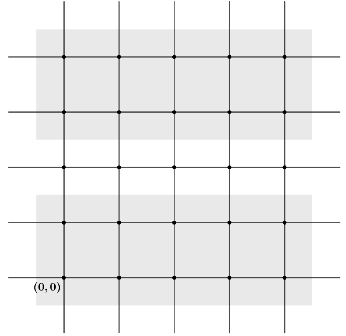
(a) $\Omega$ is the set formed by the points in the shaded region.

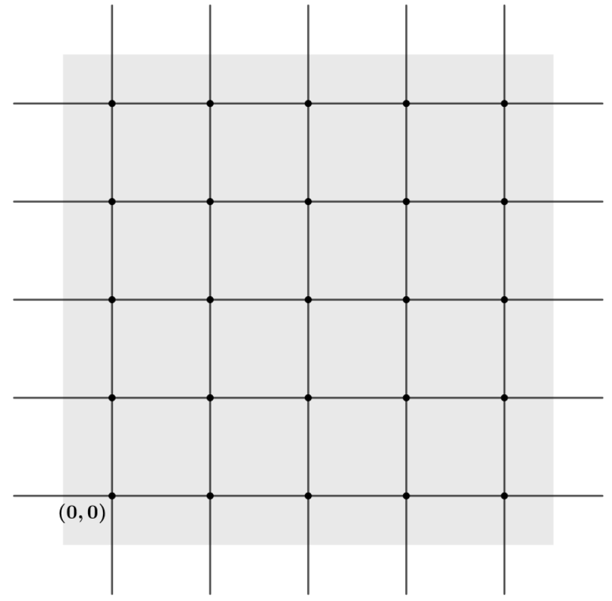
(b) The minimizer, $E$, for $\frac{1}{3}<\lambda<\frac{2}{5}$ is the set formed by the points in the shaded region.

Figure 1. The point $(0,0)$ is labelled in the graphs, and the adjacent points are represented by the dots.

3.3. The Gradient Descent Method

In order to apply this method one needs to solve the Cauchy problem

$$\left\{\begin{array}[]{ll}v_{t}\in\Delta_{1}^{m}v(t)-\lambda{\rm sign}(v(t)-f)&\hbox{in}\ (0,T)\times X\\ \\ v(0,x)=v_{0}(x)&\hbox{in}\ x\in X,\end{array}\right.$$ (3.28)

that can be rewritten as the following abstract Cauchy problem in $L^{2}(X,\nu)$

$$v^{\prime}(t)+\partial\mathcal{E}_{m}(u,f,\lambda)(v(t))\ni 0,\quad v(0)=v_{0}.$$ (3.29)

Let $f$ be in $L^{1}(X,\nu)$ . Since $\mathcal{E}_{m}(\cdot,f,\lambda)$ is convex and lower semi-continuous, by the theory of maximal monotone operators ([10]), we have that, for any initial data $v_{0}\in L^{2}(X,\nu)$, problem (3.29) has a unique strong solution. Therefore, if we define a solution of problem (3.28) as a function $v\in C(0,T;L^{2}(X,\nu))\cap W^{1,1}_{loc}(0,T;L^{2}(X,\nu))$ such that $v(0,x)=v_{0}(x)$ for $\nu$-a.e. $x\in X$ and such that there exists $\xi(t)\in{\rm sign}(v(t)-f)$ satisfying

$$\lambda\xi(t)+v_{t}(t)\in\Delta_{1}^{m}(v(t))\quad\hbox{for almost all}\ \ t\in(0,T),$$

we have the following existence and uniqueness result.

Theorem 3.38.

For every $v_{0}\in L^{2}(X,\nu)$ there exists a unique strong solution of the Cauchy problem (3.28) in $(0,T)$ for any $T>0$. Moreover, we have the following contraction principle in any $L^{q}(X,\nu)$–space, $1\leq q\leq\infty$:

$$\|v(t)-w(t)\|_{q}\leq\|v_{0}-w_{0}\|_{q}\quad\forall\,0<t<T,$$ (3.30)

for any pair of solutions $v,\,w$ of problem (3.28) with initial datum $v_{0}$, $w_{0}$ respectively.

Note that the contraction principle (3.30) in any $L^{q}$-space follows from the fact that the operator $\partial\mathcal{E}_{m}(\cdot,f,\lambda)$ is completely accretive. Indeed, given $(u_{1},v_{1}),(u_{2},v_{2})\in\partial\mathcal{E}_{m}(\cdot,f,\lambda)$ and

$$p\in P_{0}:=\{q\in C^{\infty}(\mathbb{R})\ :\ 0\leq q^{\prime}\leq 1,\ \ \hbox{supp}(q^{\prime})\ \hbox{compact and }\ 0\not\in\hbox{supp}\},$$

we need to prove that

$$\int_{X}(v_{2}-v_{1})p(u_{2}-u_{1})d\nu\geq 0.$$

Now, there exist $\xi_{i}\in{\rm sign}(u_{i}-f)$ such that $v_{i}-\lambda\xi_{i}=w_{i}\in\partial\mathcal{F}_{m}(u_{i})$, $i=1,2$. Then, since $\partial\mathcal{F}_{m}$ is a completely accretive operator and

$$\lambda\int_{X}(\xi_{2}-\xi_{1})p(u_{2}-u_{1})d\nu=\lambda\int_{X}(\xi_{2}-\xi_{1})p((u_{2}-f)-(u_{1}-f))d\nu\geq 0,$$

we have that

$$\int_{X}(v_{2}-v_{1})p(u_{2}-u_{1})d\nu=\int_{X}(w_{2}-w_{1})p(u_{2}-u_{1})+\lambda\int_{X}(\xi_{2}-\xi_{1})p(u_{2}-u_{1})d\nu\geq 0.$$

Let $(T_{\lambda}(t))_{t\geq 0}$ be the semigroup in $L^{2}(X,\nu)$ associated with the operator $\partial\mathcal{E}_{m}(\cdot,f,\lambda)$, that is, $T_{\lambda}(t)v_{0}$ is the solution of problem (3.28). On account of the contraction principle we have that for any $u^{*}\in M(f,\lambda)$, if $\mathcal{L}_{u^{*}}(u):=\|u-u^{*}\|_{2}$, then

$$\mathcal{L}_{u^{*}}\ \hbox{is a Lyapunov functional for the semigroup}\ (T_{\lambda}(t))_{t\geq 0}.$$ (3.31)

Indeed, for $t>s$, we have

$$\mathcal{L}_{u^{*}}(T_{\lambda}(t)v_{0})=\|T_{\lambda}(t)v_{0}-u^{*}\|_{2}=\|T_{\lambda}(t-s)\left(T_{\lambda}(s)v_{0}\right)-T_{\lambda}(t-s)u^{*}\|_{2}$$

$$\leq\|T_{\lambda}(s)v_{0}-u^{*}\|_{2}=\mathcal{L}_{u^{*}}(T_{\lambda}(s)v_{0}).$$

Theorem 3.39.

Assume that $f\in L^{1}X,\nu)$. Let $v_{0}\in L^{2}(X,\nu)$ and $v(t):=T_{\lambda}(t)v_{0}$. If the $\omega$-limit set

$$\omega(v_{0}):=\{w\in L^{2}(X,\nu)\ :\ \exists t_{n}\to+\infty\ s.t.\lim_{n\to\infty}v(t_{n})=w\}$$

is non-empty, then there exists $u^{*}\in M(f,\lambda)$ such that

$$\lim_{t\to\infty}v(t)=u^{*}\quad\hbox{in}\ \ L^{2}(X,\nu).$$

Proof.

Let $u^{*}\in\omega(v_{0})$, then there exists $t_{n}\to+\infty$ such that

$$\lim_{n\to\infty}v(t_{n})=u^{*}.$$

By [10, Theorem 3.2], we get

$$\frac{d^{+}v}{dt}(t)+\partial\mathcal{E}_{m}(\cdot,f,\lambda)(v(t))\ni 0\quad\hbox{for all}\ t\in(0,+\infty)$$ (3.32)

and, by Theorem 3.11, we have that $M(f,\lambda)\not=\emptyset$ thus $0\in R(\partial\mathcal{E}_{m}(\cdot,f,\lambda))$. Therefore, by [10, Theorem 3.10],

$$\lim_{n\to\infty}\frac{d^{+}v}{dt}(t_{n})=0.$$ (3.33)

Since $\partial\mathcal{E}_{m}(\cdot,f,\lambda)$ is closed, from (3.32) and (3.33) we get

$$0\in\partial\mathcal{E}_{m}(\cdot,f,\lambda)(u^{*}),$$

i.e. $u^{*}\in M(f,\lambda)$. Now, by (3.31), $\mathcal{L}_{u^{*}}$ is a Lyapunov functional for the semigroup $(T_{\lambda}(t))_{t\geq 0}$, from where it follows that

$$\lim_{t\to\infty}v(t)=u^{*}\quad\hbox{in}\ \ L^{2}(X,\nu).$$

$\Box$

Proving that the $\omega$-limit set $\omega(v_{0})$ is non-empty is not an easy task here. For example, one could try to proceed with the usual method of proving that the resolvent is compact, but this requires the use of regularity results which are difficult to obtain in our context due to the non-locality of the problem. Nonetheless, in finite graphs it is trivially true that the $\omega$-limit set is non-empty. Consequently, we have the following result.

Corollary 3.40.

Let $[X,d,m]$ be the metric random walk space associated to a connected and weighted discrete graph $G=(V(G),E(G))$. Then, for every $v_{0}\in L^{2}(X,\nu)$ and for $v(t):=T_{\lambda}(t)v_{0}$, there exists $u^{*}\in M(f,\lambda)$ such that

$$\lim_{t\to\infty}v(t)=u^{*}\quad\hbox{in}\ \ L^{2}(V(G),\nu_{G}).$$

Acknowledgment. The authors have been partially supported by the Spanish MICIU and FEDER, project PGC2018-094775-B-100. The second author was also supported by the Spanish MICIU under Grant BES-2016-079019, which is also supported by the European FSE.

References

- [1] S. Alliney, Digital Filters as Absolute Norm Regularizers. IEEE Trans. on Signal Processing, 40 (1992), 1548–1562.
- [2] S. Alliney, A Property of the Minimum Vectors of a Regularizing Functional Defined by Means of the Absolute Norm. IEEE Trans. on Signal Processing, 45 (1997), 913–917.
- [3] L. Ambrosio, N. Fusco and D. Pallara, Functions of Bounded Variation and Free Discontinuity Problems. Oxford Mathematical Monographs, 2000.
- [4] F. Andreu, V. Caselles, and J.M. Mazón, Parabolic Quasilinear Equations Minimizing Linear Growth Functionals. Progress in Mathematics, vol. 223, 2004. Birkhauser.
- [5] F. Andreu, C. Ballester, V. Caselles and J. M. Mazón, Minimizing Total Variation Flow. Differential and Integral Equations, 14 (2001), 321-360.
- [6] P. Athavale and Tadmor, Integro-Differential Equations Based on Image Decomposition. SIAM Journal on Imaging Sciences, 4 (2011), 300–312.
- [7] Ph. Bénilan and M. G. Crandall, Completely Accretive Operators. Semigroups Theory and Evolution Equations (Delft, 1989), Ph. Clement et al. editors, volume 135 of Lecture Notes in Pure and Appl. Math., Marcel Dekker, New York, 1991, pp. 41–75.
- [8] S. Bougleux, A. Elmoataz and M. Melkemi, Discrete Regularization on Weighted Graphs for Image and Mesh Filtering . Proceedings of the 1st International Conference on Scale Space and Variational Methods in Computer Vision (SSVM’07), Lecture Notes in Comput. Sci. 4485, Springer-Verlag, Berlin, 2007, pp. 128–-139.
- [9] S. Bougleux, A. Elmoataz, and M. Melkemi, Local and Nonlocal Discrete Regularization on Weighted Graphs for Image and Mesh Processing. International J. of Computer Vision, 84 (2009), 220–236.
- [10] H. Brezis, Operateurs Maximaux Monotones. North Holland, Amsterdam, 1973.
- [11] A. Buades, B. Coll, and J. M. Morel, A review of image denoising algorithms, with a new one. Multiscale Modeling and Simulation, 4 (2005), 490-–530.
- [12] A. Chambolle and P.L. Lions, Image Recovery via Total Variation Minimization and Related Problems. Numerische Mathematik 76 (1997), 167-188.
- [13] T. F. Chan and S. Esedoglu, Aspects of the Total Variation Regularized Function Approximation. SIAM Journal on Applied Mathematics, 65 (2005), 1817-1837.
- [14] T. F. Chan, S. Esedoglu, and M. Nikolova, Algorithms for Finding Global Minimizers of Image Segmentation and Denoising Models. SIAM Journal on Applied Mathematics, 66 (2006),1632–1648.
- [15] K.C. Chang, Spectrum of the -Laplacian and Cheeger’s Constant on Graphs. Journal of Graph Theory, 81 (2016), 167-207.
- [16] J. Darbon, Total Variation Minimization with Data Fidelity as a Contrast Invariant Filter. Proceedings of the 4th International Symposium on Image and Signal Processing and Analysis (ISPA 2005), 2005, 221–226.
- [17] V. Duval, J-F. Aujol and Y. Gousseau, The TVL1 Model: a Geometric Point of View . SIAM Journal on Multiscale Modeling and Simulation, 8 (2009), 154-189.
- [18] A. Elmoataz, O. Lezoray and S. Bougleux, Nonlocal discrete regularization on weighted graphs: a framework for image and manifold processing. IEEE Trans. on Image Processing, 17 (2008), 1047–1060.
- [19] N. García-Trillo and D. Slep¸ev, Continuum Limit of Total Variation on Point Clouds. Archive for Rational Mechanics and Analysis, 220 (2016), 193-241.
- [20] N. García-Trillo, D. Slep¸ev, J von Brecht, T. Laurent and X. Bresson, Consistency of Cheeger and Ratio Graph Cuts. Journal of Machine Learning Research, 17 (2016), 1-46.
- [21] G. Gilboa and S. Osher, Nonlocal Operators with Applications to Image Processing. SIAM Journal on Multiscale Modeling and Simulation, 7 (2008), 1005-1028.
- [22] Y. van Gennip, N. Guillen, B. Osting and A, Bertozzi, Mean Curvature, Threshold Dynamics, and Phase Field Theory on Finite Graphs. Milan Journal of Mathematics, 82 (2014), 3–65.
- [23] M. Hein and T. Bühler, An Inverse Power Method for Nonlinear Eigenproblems with Applications in -Spectral Clustering and Sparse PCA. Advances in neural information processing systems, 23 (2010), 847-855.
- [24] M. Hidane, O. Lézoray and A. Elmoataz, Nonlinear Multilayered Representation of Graph-Signals. Journal of Mathematical Imaging and Vision, 45 (2013),114–137
- [25] M. Hidane, O. Lézoray, V.T. Ta and A. Elmoataz, Nonlocal Multiscale Hierarchical Decomposition on Graphs. Computer Vision ECCV 2010, 638-–650. Lecture Notes in Computer Science, 6314. Springer, Berlin-Heidelberg, 2010
- [26] S. Kindermann, S. Osher and P. Jones, Deblurring and Denoising of Images by Nonlocal Functionals. SIAM Journal on Multiscale Modeling and Simulation, 4 (2005), 1091-–1115.
- [27] F. Lozes, A. Elmoataz and O. Lézoray, Partial Difference Operators on Weighted Graphs for Image Processing on Surfaces and Point Clouds. IEEE Trans. on Image Processing, 23 (2014), 3896–3909.
- [28] J. M. Mazón, J. D. Rossi and J. Toledo, Nonlocal Perimeter, Curvature and Minimal Surfaces for Measurable Sets. Journal D’Analyse Mathematique, 138 (2019), 235-279.
- [29] J. M. Mazón, J. D. Rossi and J. Toledo, Nonlocal Perimeter, Curvature and Minimal Surfaces for Measurable Sets. Frontiers in Mathematics, Birkhäser, 2019.
- [30] J. M. Mazón, M. Solera and J. Toledo, The heat flow on metric random walk spaces. J. Math. Anal. Appl. 483, 123645 (2020).
- [31] J. M. Mazón, M. Solera and J. Toledo, The total variation flow in metric random walk spaces. Calc.Var. (2020) 59:29.
- [32] Y. Meyer, Oscillating Patterns in Image Processing and Nonlinear Evolution Equations. University Lecture Series, 22. American Mathematical Society, Providence, RI, 2001.
- [33] Y. Ollivier, Ricci curvature of Markov chains on metric spaces. Journal of Functional Analysis, 256 (2009), 810–864.
- [34] L. Rudin, S. Osher and E. Fatemi, Nonlinear Total Variation based Noise Removal Algoritms. Physica D., 60 (1992), 259-268.
- [35] E. Tadmor, S. Nezzar and L. Vese, A Multiscale Image Representation Using Hierarchical Decompositions. Multiscale Modeling and Simulation, 2 (2004), 554–579.
- [36] E. Tadmor, S. Nezzar and L. Vese, Multiscale hierarchical decomposition of images with applications to deblurring, denoising and segmentation. Communications in mathematical sciences, 6 (2008), 281–307.
- [37] L. P. Yaroslavsky, Digital Picture Processing–An Introduction. Springer, Berlin, 1985.
- [38] W.Yin, D. Golfarb and S. Osher, The Total Variation Regularized Model for Multiscale Decomposition. Multiscale Modeling and Simulation, 6 (2007), 190–211.