Art: Abstraction Refinement-Guided Training for
Provably Correct Neural Networks

Abstract

Artificial Neural Networks (ANNs) have demonstrated remarkable utility in various challenging machine learning applications. While formally verified properties of their behaviors are highly desired, they have proven notoriously difficult to derive and enforce. Existing approaches typically formulate this problem as a post facto analysis process. In this paper, we present a novel learning framework that ensures such formal guarantees are enforced by construction. Our technique enables training provably correct networks with respect to a broad class of safety properties, a capability that goes well-beyond existing approaches, without compromising much accuracy. Our key insight is that we can integrate an optimization-based abstraction refinement loop into the learning process and operate over dynamically constructed partitions of the input space that considers accuracy and safety objectives synergistically. The refinement procedure iteratively splits the input space from which training data is drawn, guided by the efficacy with which such partitions enable safety verification. We have implemented our approach in a tool (Art) and applied it to enforce general safety properties on unmanned aviator collision avoidance system ACAS Xu dataset and the Collision Detection dataset. Importantly, we empirically demonstrate that realizing safety does not come at the price of much accuracy. Our methodology demonstrates that an abstraction refinement methodology provides a meaningful pathway for building both accurate and correct machine learning networks.

I Introduction

Artificial neural networks (ANNs) have emerged in recent years as the primary computational structure for implementing many challenging machine learning applications. Their success has been due in large measure to their sophisticated architecture, typically comprised of multiple layers of connected neurons (or activation functions), in which each neuron represents a possibly non-linear function over the inputs generated in a previous layer. In a supervised setting, the goal of learning is to identify the proper coefficients (i.e., weights) of these functions that minimize differences between the outputs generated by the network and ground truth, established via training samples. The ability of ANNs to identify fine-grained distinctions among their inputs through the execution of this process makes them particularly useful in a variety of diverse domains such as classification, image recognition, natural language translation, or autonomous driving.

However, the most accurate ANNs may still be incorrect. Consider, for instance, the ACAS Xu (Airborne Collision Avoidance System) application that targets avoidance of midair collisions between commercial aircraft [1], whose system is controlled by a series of ANNs to produce horizontal maneuver advisories. One example safety property states that if a potential intruder is far away and is significantly slower than one’s own vehicle, then regardless of the intruder’s and subject’s direction, the ANN controller should output a Clear-of-Conflict advisory (as it is unlikely that the intruder can collide with the subject). Unfortunately, even a sophisticated ANN handler used in the ACAS Xu system, although well-trained, has been shown to violate this property [2]. Thus, ensuring the reliability of ANNs, especially those adopted in safety-critical applications, is increasingly viewed as a necessity.

The programming languages and formal methods community has responded to this familiar, albeit challenging, problem with increasingly sophisticated and scalable verification approaches [2, 3, 4, 5] — given a trained ANN and a property, these approaches either certify that the ANN satisfies the property or identify a potential violation of the property. Unfortunately, when verification fails, these approaches provide no insight on how to effectively leverage verification counterexamples to repair complex, uninterpretable networks and ensure safety. Further, many verification approaches focus on a popular, but ultimately, narrow class of properties — local robustness — expressed over some, but not all of a network’s input space.

In this paper, we address the limitations of existing verification approaches by proposing a novel training approach for generation of ANNs that are correct-by-construction with respect to a broad class of correctness properties expressed over the network’s inputs. Our training approach integrates correctness properties into the training objective through a correctness loss function that quantifies the violation of the correctness properties. Further, to enable certification of correctness of a possibly infinite set of network behaviors, our training approach employs abstract interpretation methods [4, 6] to generate sound abstractions of both the input space and the network itself. Finally, to ensure the trained network is both correct and accurate with respect to training data, our approach iteratively refines the precision of the input abstraction, guided by the value of the correctness loss function. Our approach is sound — if the correctness loss reduces to $0$, the generated ANN is guaranteed to satisfy the associated correctness properties.

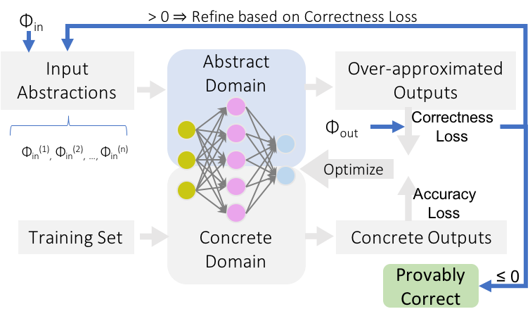
Figure 1: The Art framework.

The workflow of this overall approach — Abstraction Refinement-guided Training (Art) — is shown in Fig. 1. Art takes as input a correctness property $\left(\Phi_{\mathtt{in}},\Phi_{\mathtt{out}}\right)$ that prescribes desired network output behavior using logic constraints $\Phi_{\mathtt{out}}$ when the inputs to the network are within a domain described by $\Phi_{\mathtt{in}}$. Art is parameterized by an abstract domain $\mathcal{D}$ that yields an abstraction over inputs in $\Phi_{\mathtt{in}}$. Additionally, Art takes a set of labeled training data. The correctness loss function quantifies the distance of the abstract network output from the correctness constraint $\Phi_{\mathtt{out}}$. In each training iteration, Art both updates the network weights and refines the input abstraction. The network weights are updated using classical gradient descent optimization to mitigate the correctness loss (upper loop of Fig. 1) and the standard accuracy loss (lower loop of Fig. 1). The abstraction refinement utilizes information provided by the correctness loss to improve the precision of the abstract network output (the top arrow of Fig. 1). As we show in Section V, the key novelty of our approach - exploiting the synergy between refinement and approximation - (a) often leads to, at worst, mild impact on accuracy compared to a safe oracle baseline; and (b) provides significantly higher assurance on network correctness than existing verification or training [7] methods which do not exploit abstraction refinement.

This paper makes the following contributions. (1) We present an abstract interpretation-guided training strategy for building correct-by-construction neural networks, defined with respect to a rich class of safety properties, including functional correctness properties that relate input and output structure. (2) We define an input space abstraction refinement loop that reduces training on input data to training on input space partitions, where the precision of the abstraction is, in turn, guided by a notion of correctness loss as determined by the correctness property. (3) We formalize soundness claims that capture correctness guarantees provided by our methodology; these results characterize the ability of our approach to ensure correctness with respect to domain-specific correctness properties. (4) We have implemented our ideas in a tool (Art) and applied it to challenging benchmarks including the ACAS Xu collision avoidance dataset [1, 2] and the Collision Detection dataset [8]. We provide a detailed evaluation study quantifying the effectiveness of our approach and assess its utility to ensure correctness guarantees without compromising accuracy. We additionally provide a comparison of our approach with post facto counterexample-guided verification strategies to demonstrate the benefits of Art’s methodology compared to such techniques.

The remainder of the paper is organized as follows. In the next section, we provide a detailed motivating example that illustrates our approach. Section III provides background and Section IV formalizes our approach. Details about Art’s implementation and evaluation are provided in Section V. Related work and conclusions are presented in Section VI and VII, resp.

II Illustrative Example

We illustrate and motivate the key components of our approach by starting with a realistic, albeit simple, end-to-end example. We consider the construction of a learning-enabled system for autonomous driving. The learning objective is to identify potentially dangerous objects within a prescribed range of the vehicle’s current position.

Problem Setup. For the purpose of this example, we simplify our scenario by assuming that we track only a single object and that the information given by the vehicle’s radar is a feature vector of size two, containing (a) the object’s normalized relative speed $v\in[-5,5]$ where the positive values mean that the objects are getting closer; and (b) the object’s relative angular position $\theta\in[-\pi,\pi]$ in a polar coordinate system with our vehicle located in the center. Either action Report or action Ignore is advised by the system for this object given the information.

Consider an implementation of an ANN for this problem that uses a 2-layer ReLU neural network $F$ with initialized weights as depicted in Fig. 2. The network takes an input vector $x=\left(v,\theta\right)$ and outputs a prediction score vector $y=\left(y_{1},y_{2}\right)$ for actions Report and Ignore, respectively. The action with higher prediction score is picked by the advisory system. For simplicity, both layers in $F$ are linear layers with 2 neurons and without bias terms. An element-wise ReLU activation function $relu(x)=\max(x,0)$ is applied after the first layer.

Figure 2: A monitoring system using 2-layer ReLU network.

Correctness Property. To serve as a useful advisory system, we can ascribe some correctness properties that we would like the network to always satisfy. While our approach generalizes to an arbitrary number of the correctness properties that one may wish to enforce, we focus on one such correctness property $\Phi$ in this example: Objects in front of the vehicle that are stationary or moving closer should not be ignored. The meaning of “stationary or moving closer” and “in front of” can be interpreted in terms of predicates $\Phi_{\mathtt{in}}$ and $\Phi_{\mathtt{out}}$ over feature vector components such as $v\geq 0$ and $\theta\in[0.5,2.5]$, respectively. Using such representations and recalling that $v\in[-5,5]$, $\Phi=\left(\Phi_{\mathtt{in}},\Phi_{\mathtt{out}}\right)$ can be precisely formulated as:

$$\forall v,\theta.\;\underbrace{v\in[0,5]\ \wedge\ \theta\in[0.5,2.5]}_{\Phi_{\mathtt{in}}}\ \wedge\ y=F(v,\theta)\Rightarrow\underbrace{y_{1}>y_{2}}_{\Phi_{\mathtt{out}}}.$$

Observe that this property is violated with the network and the example input shown in Fig. 2.

Concrete Correctness Loss Function. To quantify how correct $F$ is on inputs satisfying predicate $\Phi_{\mathtt{in}}$, we define a correctness loss function, denoted $\mathit{dist}_{g}$, over the output $y$ of the neural network and the output predicate $\Phi_{\mathtt{out}}$:

$$\mathit{dist}_{g}(y,\Phi_{\mathtt{out}})=\min_{q\models\Phi_{\mathtt{out}}}g(y,q),$$

parameterized on a distance function $g$ over the input space such as the Manhattan distance ($L_{1}$-norm), Euclidean distance ($Euclid$-norm), etc. The correctness distance function is intentionally defined to be semantically meaningful—when $dist_{g}(y,\Phi_{\mathtt{out}})=0$, it follows that $y$ satisfies the output predicate $\Phi_{\mathtt{out}}$. This function can then be used as a loss function, among other training objectives to train the neural network towards satisfying $\left(\Phi_{\mathtt{in}},\Phi_{\mathtt{out}}\right)$. For this example, we can compute the correctness distance of the network output $y=\left(y_{1},y_{2}\right)$ from $\Phi_{\mathtt{out}}=y_{1}>y_{2}$ to be $dist_{Euclid}(y,\Phi_{\mathtt{out}})=\max\left((y_{2}-y_{1})/\sqrt{2},0\right)$ which is calculated based on the Euclidean distance between point $\left(y_{1},y_{2}\right)$ and line $y_{2}-y_{1}=0$.

Abstract Domain. A general correctness property like $\Phi$ is often defined over an infinite set of data points; however, since training necessarily is performed using only a finite set of samples, we cannot generalize observations made on just these samples to assert the validity of $\Phi$ on the trained network. Our approach, therefore, leverages abstract interpretation techniques to generate sound abstractions of both the network input space and the network itself. By training on these abstractions, our method obtains a finite approximation of the infinite set of possible network behaviors, enabling correct-by-construction training.

We parameterize our approach on any abstract domain that serves as a sound over-approximation of a neural network’s behavior, i.e., abstractions in which an abstract output is guaranteed to subsume all possible outputs for the set of abstract inputs. In the example, we consider the interval abstract domain $\mathcal{I}$ that is simple enough to motivate the core ideas of our approach. We note that Art is not bound to specific abstract domains, the interval domain is used only for illustrative purposes here, our experiments in Section V are conducted using more precise abstractions.

Figure 3: The 2-layer ReLU network over interval domain.

An interval abstraction of our 2-layer ReLU network, denoted $F_{\mathcal{I}}$, is shown in Fig. 3. The concrete neural network computation $F$ is abstracted by maintaining the lower and upper bounds $[\underline{u},\overline{u}]$ of each neuron $u$. For neuron $p_{2}$ in this example, following interval arithmetic [9], the lower bound of neuron is computed by $\underline{p_{2}}=1\cdot\underline{v}+(-1)\cdot\overline{\theta}=-2.5$ and the upper bound $\overline{p_{2}}=1\cdot\overline{v}+(-1)\cdot\underline{\theta}=4.5$. For ReLU activation function, $F_{\mathcal{I}}$ resets negative lower bounds to $0$ and preserves everything else. Consider neurons $p_{2}\rightarrow q_{2}$, lower bound $\underline{q_{2}}$ is reset to $0$ while its upper bound $\overline{q_{2}}$ remains unchanged. In this way, $F_{\mathcal{I}}$ soundly over-approximates all possible outputs generated by the network given any inputs satisfying $\Phi_{\mathtt{in}}$. Applying $F_{\mathcal{I}}$, the neural network’s abstract output is $y_{1}\in[-4.25,6.25]$ and $y_{2}\in[0.125,7.625]$, which fails to show that $y_{1}>y_{2}$ always holds. As a counterexample depicted in Fig. 2, the input $v=4\land\theta=1$ leads to violation.

Abstract Correctness Loss Function. Given $\Phi_{\mathtt{in}}$, to quantify how correct $F$ is based on the abstract output $y^{\#}$, we can also define an abstract correctness loss function, denoted $L_{g}$, over $y^{\#}$ and the output predicate $\Phi_{\mathtt{out}}$:

$$L_{g}(y^{\#},\Phi_{\mathtt{out}})=\max_{y\in\gamma(y^{\#})}dist_{g}(y,\Phi_{\mathtt{out}}),$$

where $\gamma(y^{\#})$ maps $y^{\#}$ to the set of values it represents in the concrete domain and $g$ is a distance function over the input space as before. In our example, $L_{Euclid}(y^{\#},\Phi_{\mathtt{out}})=\max\left((\overline{y_{2}}-\underline{y_{1}})/\sqrt{2},0\right)=11.875/\sqrt{2}$.

Measuring the worst-case distance of possible outputs to $\Phi_{\mathtt{out}}$, $L_{g}$ is also semantically meaningful — when $L_{g}(y^{\#},\Phi_{\mathtt{out}})=0$, it follows that all possible values represented by $y^{\#}$ satisfy the output predicate $\Phi_{\mathtt{out}}$. In other words, the trained neural network $F$ is certified safe w.r.t. the correctness property $\Phi$.

$L_{g}$ can be leveraged as the objective function during optimization. The $\min$ and $\max$ units in $L_{g}$ can be implemented using MaxPooling and MinPooling units, and hence is differentiable. Then we can use off-the-shelf automatic differentiation libraries [10] in the usual fashion to derive and backpropagate the gradients and readjust $F$’s weights towards minimizing $L_{g}$.

Input Space Abstraction Refinement. The abstract correctness loss function $L_{g}$ provides a direction for neural network weight optimization. However, $L_{g}$ could be overly imprecise since the amount of spurious cases introduced by the neural network abstraction is correlated with the size of the abstract input region. This kind of imprecision leads to sub-optimal optimization, ultimately hurting the feasibility of correct-by-construction as well as the model accuracy.

Such imprecision arises easily when using less precise abstract domains like the interval domain. For our running example, by bisecting the input space along each dimension, the resulting abstract correctness loss values of each region range from $3.125/\sqrt{2}$ to $9.125/\sqrt{2}$. If the original abstract correctness loss $11.875/\sqrt{2}$ pertains to a real input, it should be reflected in some sub-region as well. Now that $9.125/\sqrt{2}<11.875/\sqrt{2}$, the original abstract correctness loss must be spurious and thus suboptimal for optimization.

To use more accurate gradients for network weight optimization, our approach leverages the above observation to also iteratively partition the input region $\Phi_{\mathtt{in}}$ during training. In other words, we seek for an input space abstraction refinement mechanism that reduces imprecise abstract correctness loss introduced by abstract interpretation. Notably, incorporating input space abstraction refinement with the gradient descent optimizer does not compromise the soundness of our approach. As long as all sub-regions of $\Phi_{\mathtt{in}}$ are provably correct, the network’s correctness with respect to $\Phi_{\mathtt{in}}$ trivially holds.

Iterative Training. Our training algorithm interweaves input space abstraction refinement and gradient descent training on a network abstraction in each training iteration by leveraging the correctness loss function produced by the network abstract interpreter (as depicted in Fig. 1), until a provably correct ANN is trained. The refined input abstractions computed in an iteration are used for training over the abstract domain in the next iteration.

For our illustrative example, we set the learning rate of the optimizer to be $0.01$. In our experiment, the maximum correctness loss among all refined input space abstractions drops to $0$ after 11 iterations. Convergence was achieved by heuristically partitioning the input space $\Phi_{\mathtt{in}}$ into 76 regions. The trained ANN is guaranteed to satisfy the correctness property $(\Phi_{\mathtt{in}},\Phi_{\mathtt{out}})$.

III Background

Definition III.1 (Neural network).

Neural networks are functions $F\mathrel{\mathop{\mathchar 58\relax}}\mathbb{R}^{d}\rightarrow\mathbb{R}^{e}$ composed of $Q$ layers and $Q-1$ activation functions. Each layer is a function $f_{k}(\cdot)\in\mathbb{R}^{m_{k-1}}\rightarrow\mathbb{R}^{m_{k}}$ for $k=1,\ldots,Q$ where $m_{0}=d$ and $m_{Q}=e$. Each activation function is of the form $\sigma_{k}(\cdot)\in\mathbb{R}^{m_{k}}\rightarrow\mathbb{R}^{m_{k}}$ for $k=1,\ldots,Q-1$. Then, $F=f_{Q}\circ\sigma_{Q-1}\circ f_{Q-1}\circ\ldots\circ\sigma_{1}\circ f_{1}$.

Definition III.2 (Abstraction).

An abstraction $\mathcal{D}$ is defined as a tuple: $\left<\mathcal{D}_{c},\mathcal{D}_{a},\alpha,\gamma,T\right>$ where

• $\mathcal{D}_{c}\mathrel{\mathop{\mathchar 58\relax}}\{x~{}|~{}x\in\mathbb{R}^{d}\}$ and where $d\in\mathbb{Z}^{+}$ is the concrete domain;

• $\mathcal{D}_{a}$ is the abstract domain of interest;

• $\alpha(\cdot)$ is an abstraction function that maps a set of concrete elements to an abstract element;

• $\gamma(\cdot)$ is a concretization function that maps an abstract element to a set of concrete elements;

• $T=\left\{\left(T_{c},T_{a}\right)~{}|~{}T_{c}(\cdot)\mathrel{\mathop{\mathchar 58\relax}}\mathcal{D}_{c}\rightarrow\mathcal{D}_{c},T_{a}(\cdot)\mathrel{\mathop{\mathchar 58\relax}}\mathcal{D}_{a}\rightarrow\mathcal{D}_{a}\right\}$ is a set of transformer pairs over $\mathcal{D}_{c}$ and $\mathcal{D}_{a}$.

An abstraction is sound if for all $S\subseteq\mathcal{D}_{c}$, $S\subseteq\gamma(\alpha(S))$ holds and given $\left(T_{c},T_{a}\right)\in T$,

$$\forall c\in\mathcal{D}_{c},a\in\mathcal{D}_{a},\ c\in\gamma(a)\implies T_{c}(c)\in\gamma(T_{a}(a)).$$

Definition III.3 ($\mathcal{D}$-compatible).

Given a sound abstraction $\mathcal{D}=\left<\mathcal{D}_{c},\mathcal{D}_{a},\alpha,\gamma,T\right>$, a neural network $F$ is $\mathcal{D}$-compatible iff for every layer or activation function $\iota(\cdot)$ in $F$, there exists an abstract transformer $T_{a}$ such that $\left(\iota(\cdot),T_{a}\right)\in T$, and $T_{a}$ is differentiable at least almost everywhere.

For a $\mathcal{D}$-compatible neural network $F$, we denote by $F_{\mathcal{D}}\mathrel{\mathop{\mathchar 58\relax}}\mathcal{D}_{a}\rightarrow\mathcal{D}_{a}$ the over-approximation of $F$ where every layer $f_{k}(\cdot)$ and activation function $\sigma_{k}(\cdot)$ in $F$ are replaced in $F_{\mathcal{D}}$ by their corresponding abstract transformers in $\mathcal{D}$.

Although our approach is parametric over abstract domains, we do require every abstract transformer $T_{a}$ associated with these domains to be differentiable, so as to enable training using the worst cases over-approximated over $\mathcal{D}$ via gradient-descent style optimization algorithms.

To reason about a neural network over an abstraction $\mathcal{D}$, we need to first characterize what it means for an ANN to operate over $\mathcal{D}$.

Definition III.4 (Evaluation over Abstract Domain).

Given a $\mathcal{D}$-compatible neural network $F$, the evaluation of $F$ over $\mathcal{D}$ and a range of inputs $X\in\mathcal{D}_{a}$ is $F_{\mathcal{D}}(X)$ where $F_{\mathcal{D}}(X)$ over-approximates all possible outputs in the concrete domain corresponding to any input covered by $X$.

Theorem III.1 (Over-approximation Soundness).

For sound abstraction $\mathcal{D}$, given a $\mathcal{D}$-compatible neural network $F$, a range of inputs $X\in\mathcal{D}_{a}$,

$$\forall x.\;{x}\in\gamma(X)\,\Rightarrow\,F\left(x\right)\in\gamma\left(F_{\mathcal{D}}\left(X\right)\right).$$

Proofs of all theorems are provided in the Appendix.

IV Correct-by-Construction Training

Our approach aims to train an ANN $F$ with respect to a correctness property $\Phi$, which is formally defined in Section IV-A. The abstraction of $F$ w.r.t. $\Phi$ based on abstract domain $\mathcal{D}$ essentially can be seen as a function parameterized over the weights of $F$, which can nonetheless be trained to fit $\Phi$ using standard optimization algorithms. Section IV-B formally defines the abstract correctness loss function $L_{\mathcal{D}}$ to guide the optimization of $F$’s weights over $\mathcal{D}$. Such an abstraction inevitably introduces spurious data samples into training due to over-approximation. Section IV-C introduces the idea of input space abstraction and refinement as a mechanism that can reduce such spuriousness during optimization over $\mathcal{D}$. The detailed pseudocode of Art algorithm, including the refinement procedure, is presented in Section IV-D.

IV-A Correctness Property

The correctness properties we consider are expressed as logical propositions over the network’s inputs and outputs. We assume that an ANN correctness property expresses constraints on the outputs, given assumptions on the inputs.

Definition IV.1 (Correctness Property).

Given a neural network $F\mathrel{\mathop{\mathchar 58\relax}}\mathbb{R}^{d}\rightarrow\mathbb{R}^{e}$, a correctness property $\Phi=\left(\Phi_{\mathtt{in}},\Phi_{\mathtt{out}}\right)$ is a tuple in which $\Phi_{\mathtt{in}}$ defines a bounded input domain over $\mathbb{R}^{d}$ in the form of an interval $[\underline{x},\overline{x}]$ where $\underline{x},\overline{x}\in\mathbb{R}^{d}$, are lower, upper bounds, resp., on the network input; and $\Phi_{\mathtt{out}}$ is a quantifier-free Boolean combination of linear inequalities over the network output vector $y\in\mathbb{R}^{e}$:

• ¡$\Phi_{\mathtt{out}}$¿ ::= ¡P¿ — $\neg$¡P¿ — ¡P¿ $\land$ ¡P¿ — ¡P¿ $\lor$ ¡P¿;

  ¡P¿ ::= $A\cdot y\leq b$ where $A\in\mathbb{R}^{e},\,b\in\mathbb{R}$;

An input vector $x\in\mathbb{R}^{d}$ is said to satisfy $\Phi_{\mathtt{in}}=[\underline{x},\overline{x}]$, denoted $x\models\Phi_{\mathtt{in}}$, iff $\underline{x}\leq x\leq\overline{x}$. An output vector $y\in\mathbb{R}^{e}$ satisfies $\Phi_{\mathtt{out}}$, denoted $y\models\Phi_{\mathtt{out}}$, iff $\Phi_{\mathtt{out}}(y)$ is true. A neural network $F\mathrel{\mathop{\mathchar 58\relax}}\mathbb{R}^{d}\rightarrow\mathbb{R}^{e}$ satisfies $\Phi$, denoted $F\models\Phi$, iff $\forall x.\;x\models\Phi_{\mathtt{in}}\,\Rightarrow\,F(x)\models\Phi_{\mathtt{out}}$.

Definition IV.2 (Concrete Correctness Loss Function).

For an atomic output predicate $P$, the concrete correctness loss function, $dist_{g}(y,P)$, quantifies the distance from an output vector $y\in\mathbb{R}^{e}$ to $P$:

$$dist_{g}(y,P)=\min_{q\models P}g(y,q)$$

where $g\mathrel{\mathop{\mathchar 58\relax}}\mathbb{R}^{d}\times\mathbb{R}^{d}\mapsto\mathbb{Z}^{\geq 0}$ is a differentiable distance function over the inputs. Similarly, $dist_{g}(y,\Phi_{\mathtt{out}})$, the “distance” from an output vector $y\in\mathbb{R}^{e}$ to general output predicate $\Phi_{\mathtt{out}}$, can be computed efficiently by induction as long as $g(\cdot,\cdot)$ can be computed efficiently:

• $dist_{g}(y,P)$ and $dist_{g}(y,\neg P)$ can be computed using basic arithmetic;

• $dist_{g}(y,P_{1}\land P_{2})$ = $\max(dist_{g}(y,P_{1}),dist_{g}(y,P_{2}))$;

• $dist_{g}(y,P_{1}\lor P_{2})$ = $\min(dist_{g}(y,P_{1}),dist_{g}(y,P_{2}))$.

Note that $dist_{g}(y,\Phi_{\mathtt{out}})$ may not represent the minimum distance for arbitrary $\Phi_{\mathtt{out}}$, but it is efficient to compute while still retaining the following soundness theorem.

Theorem IV.1 (Zero Concrete Correctness Loss Soundness).

Given output predicate $\Phi_{\mathtt{out}}$ over $\mathbb{R}^{e}$ and output vector $y\in\mathbb{R}^{e}$,

$$dist_{g}(y,\Phi_{\mathtt{out}})=0\implies y\models\Phi_{\mathtt{out}}.$$

IV-B Over-approximation

To reason about correctness properties defined over an infinite set of data points, our approach generates sound abstractions of both the network input space and the network itself, obtaining a finite approximation of the infinite set of possible network behaviors. We start by quantifying the abstract correctness loss of over-approximated outputs.

Definition IV.3 (Abstract Correctness Loss Function).

Given a sound abstraction $\mathcal{D}=\left<\mathcal{D}_{c},\mathcal{D}_{a},\alpha,\gamma,T\right>$, a $\mathcal{D}$-compatible neural network $F$, and a correctness property $\Phi=\left(\Phi_{\mathtt{in}},\Phi_{\mathtt{out}}\right)$, the abstract correctness loss function is defined as:

$$\begin{split}L_{\mathcal{D},g}(F,\Phi)&=\max_{p\in\gamma(Y_{\mathcal{D}})}dist_{g}(p,\Phi_{\mathtt{out}})\\ \text{where }Y_{\mathcal{D}}&=F_{\mathcal{D}}(\alpha(\Phi_{\mathtt{in}})).\end{split}$$

Here $g\mathrel{\mathop{\mathchar 58\relax}}\mathbb{R}^{d}\times\mathbb{R}^{d}\mapsto\mathbb{Z}^{\geq 0}$ is a differentiable distance function over concrete inputs as before.

The abstract correctness loss function measures the worst-case distance to $\Phi_{\mathtt{out}}$ of any neural network outputs subsumed by the abstract network output. It is designed to extend the notion of concrete correctness loss to the abstract domain with a similar soundness guarantee, as formulated in the following theorem.

Theorem IV.2 (Zero Abstract Correctness Loss Soundness).

Given a sound abstraction $\mathcal{D}$, a $\mathcal{D}$-compatible neural network $F$, and a correctness property $\Phi$,

$$L_{\mathcal{D},g}(F,\Phi)=0\implies F\models\Phi.$$

In what follows, we fix the distance function $g$ over concrete inputs and denote the abstract correctness loss function simply as $L_{\mathcal{D}}$.

IV-C Abstraction Refinement

Recall that in Section II we illustrated how imprecision in the correctness loss for a coarse abstraction can be mitigated using an input space abstraction refinement mechanism. Our notion of refinement is formally defined below.

Definition IV.4 (Input Space Abstraction).

An input space abstraction $S$ refines a correctness property $\Phi=\left(\Phi_{\mathtt{in}},\Phi_{\mathtt{out}}\right)$ into a set of correctness properties $S=\left\{\left(\Phi^{i}_{\mathtt{in}},\Phi_{\mathtt{out}}\right)\right\}$ such that $\Phi_{\mathtt{in}}=\bigcup_{i}\Phi^{i}_{\mathtt{in}}$. Given a neural network $F$ and an input space abstraction $S$, $F\models S\iff\bigwedge_{\Phi\in S}F\models\Phi$.

Definition IV.5 (Input Space Abstraction Refinement).

A well-founded abstraction refinement $\sqsubseteq$ is a binary relation over a set of input abstractions $\mathcal{S}=\{S_{1},S_{2},\ldots\}$ such that:

• (reflexivity): $\forall S_{i}\in\mathcal{S}$, $\,S_{i}\sqsubseteq S_{i}$;

• (refinement): $\forall S_{i}\in\mathcal{S}$ and correctness property $(\Psi_{\mathtt{in}},\Psi_{\mathtt{out}})$,

  $$\begin{split}&\left(\Psi_{\mathtt{in}}=\bigcup_{(\Phi^{j}_{\mathtt{in}},\_)\in S_{i}}\Phi^{j}_{\mathtt{in}}\right)\land\left(\bigwedge_{(\_,\Phi^{j}_{\mathtt{out}})\in S_{i}}\Phi^{j}_{\mathtt{out}}\Leftrightarrow\Psi_{\mathtt{out}}\right)\\ &\implies S_{i}\sqsubseteq\{(\Psi_{\mathtt{in}},\Psi_{\mathtt{out}})\};\end{split}$$

• (transitivity): $\forall S_{1},S_{2},S_{3}\in\mathcal{S}$, $S_{1}\sqsubseteq S_{2}\land S_{2}\sqsubseteq S_{3}\implies S_{1}\sqsubseteq S_{3}$;

• (composition): $\forall S_{1},S_{2},S_{3},S_{4}\in\mathcal{S},S_{1}\sqsubseteq S_{3}\land S_{2}\sqsubseteq S_{4}\implies S_{1}\cup S_{2}\sqsubseteq S_{3}\cup S_{4}$.

The reflexivity, transitivity, and compositional requirements for a well-founded refinement are natural. The refinement rule states that an input space abstraction $S$ refines some correctness property $\left(\Psi_{\mathtt{in}},\Psi_{\mathtt{out}}\right)$ if the union of all input domains in $S$ is equivalent to $\Psi_{\mathtt{in}}$ and all output predicates in $S$ are logically equivalent to $\Psi_{\mathtt{out}}$. This rule enables $\Psi_{\mathtt{in}}$ to be safely decomposed into a set of sub-domains. As a result, the problem of enforcing coarse-grained correctness properties on neural networks can be converted into one that enforces multiple fine-grained properties, an easier problem to tackle because much of the imprecision introduced by the coarse-grained abstraction can now be eliminated.

Theorem IV.3 (Sufficient Condition via Refinement).

$$\forall F,S_{1},S_{2},~{}S_{1}\sqsubseteq S_{2}\land F\models S_{1}\implies F\models S_{2}.$$

To do this, we naturally extend the notion of abstract correctness loss over one property to an input space abstraction.

Definition IV.6 (Abstract Correctness Loss Function for Input Space Abstraction).

Given a sound abstraction $\mathcal{D}$, $\mathcal{D}$-compatible neural network $F$, and input space abstraction $S$, the abstract correctness loss of $F$ with respect to $S$ is denoted by

$$L_{\mathcal{D}}(F,S)=\sum_{\Phi\in S}L_{\mathcal{D}}(F,\Phi).$$

Theorem IV.4 (Zero Abstract Correctness Loss for Input Space Abstraction).

Given a sound abstraction $\mathcal{D}$, a $\mathcal{D}$-compatible neural network $F$, and an input space abstraction $S$,

$$L_{\mathcal{D}}(F,S)=0\implies F\models S.$$

IV-D The Art Algorithm

Figure 4: Art correct-by-construction training algorithm.

1:Abstract domain $\mathcal{D}$, $\mathcal{D}$-compatible neural network $F$, input space abstraction $S$, learning rate $\eta\in\mathbb{R}^{+}$, training data set $\{(x_{\text{train}},y_{\text{label}})\}$, accuracy loss function $L_{\mathcal{A}}$, accuracy loss bound $\epsilon_{\mathcal{A}}\in\mathbb{R}^{+}$, hyper-parameter $k$.

2:Return the optimized $F$ whose correctness properties are enforced and accuracy loss bounded by $\epsilon_{\mathcal{A}}$.

3:

4:procedure Art

5:     $\vec{W}\leftarrow$ all weights in $F$ to optimize

6:     while true do

7:          $\ell_{\mathcal{D}},\ \ell_{\mathcal{A}}\leftarrow L_{\mathcal{D}}(F,S),\ L_{\mathcal{A}}(F,\{(x_{\text{train}},y_{\text{label}})\})$

8:         if $\ell_{\mathcal{D}}=0\ \wedge\ \ell_{\mathcal{A}}\leq\epsilon_{\mathcal{A}}$ then

9:              return $F$ 

10:         end if

11:$\triangleright$ optimization

12:          $\nabla F\leftarrow\frac{\partial(\ell_{\mathcal{D}}+\ell_{\mathcal{A}})}{\partial\vec{W}}$ 

13:         $\vec{W}\leftarrow\vec{W}-\eta\cdot\nabla F$ 

14:$\triangleright$ refinement

15:         $T\leftarrow$ Subset of $S$ with $k$ largest $\ell_{\mathcal{D}}$ values

16:         $S^{\prime}\leftarrow S\setminus T$

17:         for all $(\Phi^{i}_{\mathtt{in}},\Phi^{i}_{\mathtt{out}})\in T$ do

18:              for all $\Psi^{j}_{\mathtt{in}}\in$ Refine($\Phi^{i}_{\mathtt{in}}$, $\ell_{\mathcal{D}}$) do

19:                  $S^{\prime}\leftarrow S^{\prime}\cup\{(\Psi^{j}_{\mathtt{in}},\Phi^{i}_{\mathtt{out}})\}$ 

20:              end for

21:         end for

22:         $S\leftarrow S^{\prime}$ 

23:     end while

24:end procedure

25:

26:procedure Refine($\Psi_{\mathtt{in}}$, $\ell_{\mathcal{D}}$)

27:     for all dimension $i$ of $\Psi_{\mathtt{in}}$ do

28:         score${}_{i}=\frac{\partial\ell_{\mathcal{D}}}{\partial\{\Psi_{\mathtt{in}}\}_{i}}\times|\{\Psi_{\mathtt{in}}\}_{i}|$

29:     end for

30:     $dim\leftarrow\arg\max\text{score}_{i}$ $\triangleright$ pick dimension

31:     $\Psi_{\mathtt{in}}^{1},\Psi_{\mathtt{in}}^{2}\leftarrow\Psi_{\mathtt{in}}$ bisected along dimension $dim$

32:     return $\left\{\Psi_{\mathtt{in}}^{1},\Psi_{\mathtt{in}}^{2}\right\}$

33:end procedure

The goal of our ANN training algorithm, given in Fig. 4, is to optimize the network to have $L_{\mathcal{D}}(F,S)$ reduce to $0$, thereby ensuring a correct-by-construction network. The algorithm takes as input both an initial input space abstraction $S$ and a set of labeled training data $\left\{\left(x_{\text{train}},y_{\text{label}}\right)\right\}$ in order to achieve correctness while maintaining high accuracy on the trained model. The abstract correctness loss, denoted $\ell_{\mathcal{D}}$, is computed at Line 7 according to Def. IV.3 and checked correctness by comparing against $0$. If $\ell_{\mathcal{D}}=0$, as long as the accuracy loss, denoted $\ell_{\mathcal{A}}$, is also satisfactory, Art returns a correct and accurate network following Thm. IV.4.

The joint loss of $\ell_{\mathcal{D}}$ and $\ell_{\mathcal{A}}$ is used to guide the optimization of neural network parameters using standard gradient-descent algorithms. The requirement of abstract transformers being differentiable at least almost anywhere in Def. III.3 enables computation of gradients $\ell_{\mathcal{D}}$ using off-the-shelf automatic differentiation libraries [10].

Starting from Line 15, abstractions in $S$ that have the largest $\ell_{\mathcal{D}}$ values represent the potentially most imprecise cases and thus are chosen for refinement. During refinement, Art first picks a dimension to refine using heuristic scores similar to [3]. The heuristic coarsely approximates the cumulative gradient over one dimension, with a larger score suggesting greater potential of decreasing correctness loss. The input abstraction is then bisected along the picked dimension as refinement.

Corollary 1 (Art Soundness).

Given a sound abstraction $\mathcal{D}$, a $\mathcal{D}$-compatible neural network $F$, and an initial input space abstraction $S$ of correctness properties, if the Art algorithm in Fig. 4 generates a neural network $F^{\prime}$, $L_{\mathcal{D}}(F^{\prime},S)=0$ and $F^{\prime}\models S$.

V Evaluation

We have performed an evaluation of our approach to validate the feasibility of building neural networks that are correct-by-construction over a range of correctness properties. All experiments reported in this section were performed on a Ubuntu 16.04 system with 3.2GHz CPU and NVidia GTX 1080 Ti GPU with 11GB memory. All experiments uses the DeepPoly abstract domain [11] implemented on Python 3.7 and PyTorch 1.4 [10].

V-A ACAS Xu Dataset

Our first evaluation study centers around the network architecture and correctness properties described in the Airborne Collision Avoidance System for Unmanned Aircraft (ACAS Xu) dataset [1, 2]. A family of $45$ neural networks are used in the avoidance system; each of these networks consists of $6$ hidden layers with $50$ neurons in each hidden layer. ReLU activation functions are applied to all hidden layer neurons. All $45$ networks take a feature vector of size $5$ as input that encodes various aspects of an airborne environment. The outputs of the networks are prediction scores over $5$ advisory actions to select the advisory action.

In the evaluation, we reason about sophisticated correctness conditions of the ACAS Xu system in terms of its aggregated ability to preserve up to $10$ correctness properties [2] among all $45$ networks. Each network is supposed to satisfy some subset of these $10$ properties. All correctness properties $\Phi$ can be formulated in terms of input ($\Phi_{\mathtt{in}}$) and output ($\Phi_{\mathtt{out}}$) predicates as in Section IV-A.

Setup. Among the $45$ provided networks, $36$ are reported with safety property violations and $9$ are reported safe [2]. We evaluate Art on those $36$ unsafe networks to demonstrate the effectiveness of generating correct-by-construction networks. The test sets from unsafe networks may contain unsafe points and are thus unauthentic, so we apply Art on those $9$ already safe networks to demonstrate the accuracy overhead when enforcing the safety properties. Unfortunately, the training and test sets to build these ACAS Xu networks are not publicly available online. In spite of that, the ACAS Xu dataset provides the state space of input states that is used for training and over which the correctness properties are defined. We, therefore, uniformly sample a total of $10$k training set and $5$k test set data points from the state space. The labels are collected by evaluating each of the provided $45$ networks on these sampled inputs, with those ACAS Xu networks serving as oracles. Each network is then trained by Art using its safety specification and the prepared training set, starting with the provided weights when available or otherwise randomly initialized weights. We record whether the trained network is correct-by-construction, as well as their accuracy evaluated on the prepared test set and the overall training time.

Applying Art. During each training epoch (i.e., each iteration of the outermost while loop in Fig. 4), our implementation refines up to $k=200$ abstractions at a time that expose the largest correctness losses. Larger $k$ leads to finer-grained abstractions but incurs more training cost. The Adam optimizer [12] is used in both training tasks and runs up to $100$ epochs with learning rate $0.001$ and a learning rate decay policy if the loss has been stable for some time. Cross entropy loss is used as the loss function for accuracy . For all experiments with refinement enabled, refinement operations are applied to derive up to $5$k refined input space abstractions before weight update starts. The detailed results are shown in Table I.

TABLE I: Applying Art to ACAS Xu Dataset.

	Refinement	Safe%	Min Accu.	Mean Accu.	Max Accu.
$36$ unsafe nets	Yes No	100% $94.44\%$	$90.38\%$ $87.88\%$	$96.10\%$ $94.45\%$	$98.70\%$ $98.22\%$
$9$ safe nets	Yes No	100% $88.89\%$	$93.82\%$ $86.32\%$	$96.25\%$ $94.29\%$	$99.92\%$ $99.92\%$

To demonstrate the importance of abstraction refinement mechanism, we also compare between the results with and without refinement (as done in existing work [6]). For completeness, we record the correct-by-construction enforced rate (Safe%) and the evaluated accuracy statistics for both tasks among multiple runs. Observe that Art successfully generates correct-by-construction networks for all scenarios with only minimal loss in accuracy. On the other hand, if refinement is disabled, it fails to generate correct-by-construction networks for all cases, and displays lower accuracy than the refinement-enabled instantiations. The average training time for each network is 69.39s if with refinement and 57.85s if without.

Figure 5: Correctness rate and accuracy change of post facto training using sampled points or counterexamples. Results are normalized based on the baseline networks.

Comparison with post facto training loop. We also consider a comparison of our abstraction refinement-guided training for correct-by-construction networks against a post facto training loop that feed concrete correctness related data points to training loops. Such concrete points may be sampled from the provided specification or the collected counterexamples from an external solver. We show the results on $8$ representative networks comparing to the same baseline in Figure 5. These $8$ networks belong to a representative set of networks that cover all $10$ provided safety properties.

For the experiment using sampled data points, $5$k points sampled from correctness properties are used during training. For the experiment using counterexamples, all counterexamples from correctness queries to external verifier ReluVal [3] are collected and used during training. In both experiments, the points from original training set are used for jointly training to preserve accuracy and the correctness distance functions following that in Section IV-B are used as loss functions. We concluded the experiments using counterexamples after $20$ epochs since no improvement was seen after this point. Both experiments fail to enforce correctness properties in most cases and they may impose great impact to model accuracy compared to the baseline network. We believe this result demonstrates the difficulty of applying a counterexample-guided training loop strategy for generating safe networks compared an abstraction-guided methodology.

V-B Collision Detection Dataset

Our second evaluation task focuses on the Collision Detection Dataset [8] where a neural network controller is used to predict whether two vehicles running curve paths at different speeds would collide. The network takes as input a feature vector of size $6$, containing the information of distances, speeds, and directions of the two vehicle. The network output prediction score are used to classify the scenario as a colliding or non-colliding case.

A total of $500$ correctness properties are proposed in the Collision Detection dataset that identify the safety margins around particular data points. The network presented in the dataset respects $328$ such properties. In our evaluation, we use a 3-layer fully-connected neural network controller with 50, 128, 50 neurons in different hidden layers. Using the same training configurations as in Section V-A and evaluating on the same training and test sets provided in the dataset, the results are shown in Table II.

TABLE II: Applying Art to Collision Detection Dataset.

	Refinement	Enforced	Accuracy	Time
Original [8]	N/A	328/500	99.87%	N/A
Art	Yes No	481/500 420/500	96.83% 86.3%	583s 419s

After $100$ epochs, Art converged to a local minimum and managed to certify $481$ out of all $500$ safety properties. Although it did not achieve zero correctness loss, ART can produce a solution that satisfies significantly more correctness properties than the oracle neural network, at the cost of only a small accuracy drop.

VI Related Work

Neural Network Verification. Inspired by the success of applying program analysis to large software code bases, abstract interpretation-based techniques have been adapted to reason about ANNs by developing efficient abstract transformers that relax nonlinearity of activation functions into linear inequality constraints [8, 13, 14, 11, 4, 7, 6]. Similar approaches [15, 16, 17, 18] encode nonlinearity via linear outer bounds of activation functions and may delegate the verification problem to SMT solvers[2, 19] or Mixed Integer Programming solvers [20, 21, 22]. Most of those verifiers focus on robustness properties only and do not support verifiable training of network-wide correctness properties. For example, [11] encodes concrete ANN operations into ELINA [23], a numeric abstract transformer, and therefore disables opportunities for training or optimization thereafter.

Correctness properties may also be retrofitted onto a trained neural network for safety concerns [24, 25, 26, 27]. These approaches usually synthesize a reactive system that monitors the potentially controller network and corrects any potentially unsafe actions. Comparing to correct-by-construction methods, runtime overheads are inevitable for such post facto shielding techniques.

Correctness Properties in Neural Networks. There have been a large number of recent efforts that have explored verifying the robustness of networks against adversarial attacks [28, 29, 30]. Recent work has shown how symbolic reasoning approaches [3, 4] can be used to help validate network robustness; other efforts combine optimization techniques with symbolic reasoning to guide symbolic analysis [5]. Our approach looks at the problem of verification and certification from the perspective of general safety specifications that are typically richer than notions of robustness governing these other techniques and provide the correct-by-construction guarantee upon training termination. Encoding logical constraints other than robustness properties into loss functions has been explored in [31, 32, 33, 34]. However, they operate only on concrete sample instances and do not provide any correct-by-construction guarantees.

Training over Abstract Domains. The closest approach to our setting is the work in [6, 35]. They introduced geometric abstractions that bound activations as they propagate through the network via abstract interpretation. Importantly, since these convex abstractions are differentiable, neural networks can optimize towards much tighter bounds to improve the verified accuracy. A simple bounding technique based on interval bound propagation was also exploited in [7] (similar to the interval domain from [6]) to train verifiably robust neural networks that even beat the state-of-the-art networks in image classification tasks, demonstrating that a correct-by-construction approach can indeed save the need of more expensive verification procedures in challenging domains. They did not, however, consider verification in the context of global safety properties as discussed here, in which the over-approximation error becomes non-negligible; nor did they formulate their approach to be parametric in the specific form of the abstractions chosen. Similar ideas have been exploited in provable defenses works [36, 37, 38, 35], however, they apply best-effort adversarial defenses only and provide no guarantee upon training termination.

VII Conclusions

This paper presents a correct-by-construction toolchain that can train neural networks with provable guarantees. The key idea is to optimize a neural network over the abstraction of both the input space and the network itself using abstraction refinement mechanisms. Experimental results show that our technique realizes trustworthy neural network systems for a variety of properties and benchmarks with only mild impact on model accuracy.

Appendix A Appendix

A-A Proofs

See III.1

Proof.

Straightforward after unfolding Definition III.2 and applying the properties of concrete and abstract transformers. ∎

See IV.1

Proof.

Straightforward after unfolding Definition IV.2 and applying the fact that distance function $g(\cdot,\cdot)\geq 0$ always holds. ∎

See IV.2

Proof.

When $L_{\mathcal{D}}(F,\Phi_{\mathtt{in}},\Phi_{\mathtt{out}})=0$, by Definition IV.3,

$$\max_{p\in\gamma(F_{\mathcal{D}}(\alpha(\Phi_{\mathtt{in}})))}dist(p,\Phi_{\mathtt{out}})=0.$$

Since $dist(\cdot)$ is a non-negative function, we have:

$$\forall p\in\gamma(F_{\mathcal{D}}(\alpha(\Phi_{\mathtt{in}}))),~{}dist(p,\Phi_{\mathtt{out}})=0.$$

By Definition III.2, we have $\Phi_{\mathtt{in}}\subseteq\gamma(\alpha(\Phi_{\mathtt{in}}))$. By Theorem III.1, we have

$$\forall x,~{}x\models\Phi_{\mathtt{in}}\implies F(x)\in\gamma(F_{\mathcal{D}}(\alpha(\Phi_{\mathtt{in}}))).$$

Hence,

$$\forall x,~{}x\models\Phi_{\mathtt{in}}\implies dist(F(x),\Phi_{\mathtt{out}})=0.$$

By Theorem IV.1, it means

$$\forall x,~{}x\models\Phi_{\mathtt{in}}\implies F(x)\models\Phi_{\mathtt{out}}.$$

Thereby proved $L_{\mathcal{D}}(F,\Phi_{\mathtt{in}},\Phi_{\mathtt{out}})=0\implies F\models(\Phi_{\mathtt{in}},\Phi_{\mathtt{out}})$. ∎

See IV.3

Proof.

By induction on Definition IV.5,

• When $S_{1}=S_{2}$, obviously $F\models S_{2}$;

• When $S_{2}=\left\{\Phi=\left(\Phi_{\mathtt{in}},\Phi_{\mathtt{out}}\right)\right\}$:

  By Definition IV.4, from $F\models S_{1}$ we have

  $$\bigwedge_{(\Psi_{\mathtt{in}},\Psi_{\mathtt{out}})\in S_{1}}F\models(\Psi_{\mathtt{in}},\Psi_{\mathtt{out}})$$

  From

  $$\bigwedge_{(\_,\Psi_{\mathtt{out}})\in S_{1}}\Psi_{\mathtt{out}}=\Phi_{\mathtt{out}}$$

  we have

  $$\bigwedge_{(\Psi_{\mathtt{in}},\Psi_{\mathtt{out}})\in S_{1}}F\models(\Psi_{\mathtt{in}},\Phi_{\mathtt{out}})$$

  Now that

  $$\Phi_{\mathtt{in}}=\bigcup_{(\Psi_{\mathtt{in}},\_)\in S_{1}}\Psi_{\mathtt{in}},$$

  by Definition IV.4, we have $F\models(\Phi_{\mathtt{in}},\Phi_{\mathtt{out}})$. Thus $F\models S_{2}$.

• For transitivity rule, by induction hypothesis.

• For composition rule, by induction hypothesis.

All cases proved. ∎

See IV.4

Proof.

Unfold the definitions, the proof is straightforward after applying Theorem IV.2 and the fact that all abstract correctness losses are non-negative. ∎

Lemma A.1 (Valid Refinement).

For any input space abstraction $S$, the code snippet of Fig. 4 starting from Line 15 to Line 22 yields an input space abstraction $S^{\prime}$ such that $S^{\prime}\sqsubseteq S$.

Proof.

In the code snippet, original input space abstraction is divided into two parts, $T$ and $S^{\prime}$. $S^{\prime}$ remains the same throughout execution, so $S^{\prime}\sqsubseteq S^{\prime}$.

For each correctness property $\left(\Phi_{\mathtt{in}},\Phi_{\mathtt{out}}\right)$ in $T$, the Refine procedure in Fig. 4 is called to generate two new input predicates $\Phi_{\mathtt{in}}^{1}$ and $\Phi_{\mathtt{in}}^{2}$. It is easy to show that $\Phi_{\mathtt{in}}^{1}\cup\Phi_{\mathtt{in}}^{2}=\Phi_{\mathtt{in}}$. So every new pair

$$\left\{\left(\Phi_{\mathtt{in}}^{1},\Phi_{\mathtt{out}}\right),\left(\Phi_{\mathtt{in}}^{2},\Phi_{\mathtt{out}}\right)\right\}\sqsubseteq\left\{\left(\Phi_{\mathtt{in}},\Phi_{\mathtt{out}}\right)\right\}.$$

By composition rule of Definition IV.5, the union of $S^{\prime}$ and every such new pair refines original $S$. ∎

See 1

Proof.

From Lemma A.1, we know for any input space abstraction $S^{\prime}$ generated during the execution of Fig. 4, $S^{\prime}\sqsubseteq S$. Then by Theorem IV.4 and Theorem IV.3, we have

$$L_{\mathcal{D}}(F,S^{\prime})=0\implies F\models S^{\prime}\implies F\models S.$$

∎

References

- [1] K. D. Julian, J. Lopez, J. S. Brush, M. P. Owen, and M. J. Kochenderfer, “Policy compression for aircraft collision avoidance systems,” in 2016 IEEE/AIAA 35th Digital Avionics Systems Conference (DASC), Sep. 2016, pp. 1–10.
- [2] G. Katz, C. W. Barrett, D. L. Dill, K. Julian, and M. J. Kochenderfer, “Reluplex: An efficient SMT solver for verifying deep neural networks,” in Computer Aided Verification - 29th International Conference, CAV 2017, Heidelberg, Germany, July 24-28, 2017, Proceedings, Part I, 2017, pp. 97–117. [Online]. Available: https://doi.org/10.1007/978-3-319-63387-9_5
- [3] S. Wang, K. Pei, J. Whitehouse, J. Yang, and S. Jana, “Formal security analysis of neural networks using symbolic intervals,” in 27th USENIX Security Symposium, USENIX Security 2018, Baltimore, MD, USA, August 15-17, 2018., 2018, pp. 1599–1614. [Online]. Available: https://www.usenix.org/conference/usenixsecurity18/presentation/wang-shiqi
- [4] T. Gehr, M. Mirman, D. Drachsler-Cohen, P. Tsankov, S. Chaudhuri, and M. T. Vechev, “AI2: safety and robustness certification of neural networks with abstract interpretation,” in 2018 IEEE Symposium on Security and Privacy, SP 2018, Proceedings, 21-23 May 2018, San Francisco, California, USA, 2018, pp. 3–18. [Online]. Available: https://doi.org/10.1109/SP.2018.00058
- [5] G. Anderson, S. Pailoor, I. Dillig, and S. Chaudhuri, “Optimization and abstraction: a synergistic approach for analyzing neural network robustness,” in Proceedings of the 40th ACM SIGPLAN Conference on Programming Language Design and Implementation, PLDI 2019, Phoenix, AZ, USA, June 22-26, 2019., 2019, pp. 731–744. [Online]. Available: https://doi.org/10.1145/3314221.3314614
- [6] M. Mirman, T. Gehr, and M. T. Vechev, “Differentiable abstract interpretation for provably robust neural networks,” in Proceedings of the 35th International Conference on Machine Learning, ICML 2018, Stockholmsmässan, Stockholm, Sweden, July 10-15, 2018, 2018, pp. 3575–3583. [Online]. Available: http://proceedings.mlr.press/v80/mirman18b.html
- [7] S. Gowal, K. D. Dvijotham, R. Stanforth, R. Bunel, C. Qin, J. Uesato, R. Arandjelovic, T. Mann, and P. Kohli, “Scalable verified training for provably robust image classification,” in The IEEE International Conference on Computer Vision (ICCV), October 2019.
- [8] R. Ehlers, “Formal verification of piece-wise linear feed-forward neural networks,” in Automated Technology for Verification and Analysis - 15th International Symposium, ATVA 2017, Pune, India, October 3-6, 2017, Proceedings, 2017, pp. 269–286. [Online]. Available: https://doi.org/10.1007/978-3-319-68167-2_19
- [9] R. E. Moore, R. B. Kearfott, and M. J. Cloud, Introduction to Interval Analysis. SIAM, 2009. [Online]. Available: https://doi.org/10.1137/1.9780898717716
- [10] A. Paszke, S. Gross, F. Massa, A. Lerer, J. Bradbury, G. Chanan, T. Killeen, Z. Lin, N. Gimelshein, L. Antiga, A. Desmaison, A. Köpf, E. Yang, Z. DeVito, M. Raison, A. Tejani, S. Chilamkurthy, B. Steiner, L. Fang, J. Bai, and S. Chintala, “Pytorch: An imperative style, high-performance deep learning library,” in Advances in Neural Information Processing Systems 32: Annual Conference on Neural Information Processing Systems 2019, NeurIPS 2019, 8-14 December 2019, Vancouver, BC, Canada, 2019, pp. 8024–8035. [Online]. Available: http://papers.nips.cc/paper/9015-pytorch-an-imperative-style-high-performance-deep-learning-library
- [11] G. Singh, T. Gehr, M. Püschel, and M. T. Vechev, “An Abstract Domain for Certifying Neural Networks,” PACMPL, vol. 3, no. POPL, pp. 41:1–41:30, 2019. [Online]. Available: https://dl.acm.org/citation.cfm?id=3290354
- [12] D. P. Kingma and J. Ba, “Adam: A method for stochastic optimization,” in 3rd International Conference on Learning Representations, ICLR 2015, San Diego, CA, USA, May 7-9, 2015, Conference Track Proceedings, 2015. [Online]. Available: http://arxiv.org/abs/1412.6980
- [13] G. Singh, T. Gehr, M. Mirman, M. Püschel, and M. T. Vechev, “Fast and effective robustness certification,” in Advances in Neural Information Processing Systems 31: Annual Conference on Neural Information Processing Systems 2018, NeurIPS 2018, 3-8 December 2018, Montréal, Canada., 2018, pp. 10 825–10 836. [Online]. Available: http://papers.nips.cc/paper/8278-fast-and-effective-robustness-certification
- [14] G. Singh, T. Gehr, M. Puschel, and M. Vechev, “Robustness certification with refinement,” in International Conference on Learning Representations, 2019. [Online]. Available: https://openreview.net/forum?id=HJgeEh09KQ
- [15] H. Zhang, T. Weng, P. Chen, C. Hsieh, and L. Daniel, “Efficient neural network robustness certification with general activation functions,” in Advances in Neural Information Processing Systems 31: Annual Conference on Neural Information Processing Systems 2018, NeurIPS 2018, 3-8 December 2018, Montréal, Canada., 2018, pp. 4944–4953. [Online]. Available: http://papers.nips.cc/paper/7742-efficient-neural-network-robustness-certification-with-general-activation-functions
- [16] T. Weng, H. Zhang, H. Chen, Z. Song, C. Hsieh, L. Daniel, D. S. Boning, and I. S. Dhillon, “Towards fast computation of certified robustness for relu networks,” in Proceedings of the 35th International Conference on Machine Learning, ICML 2018, Stockholmsmässan, Stockholm, Sweden, July 10-15, 2018, 2018, pp. 5273–5282. [Online]. Available: http://proceedings.mlr.press/v80/weng18a.html
- [17] S. Wang, Y. Chen, A. Abdou, and S. Jana, “Mixtrain: Scalable training of formally robust neural networks,” CoRR, vol. abs/1811.02625, 2018. [Online]. Available: http://arxiv.org/abs/1811.02625
- [18] S. Wang, K. Pei, J. Whitehouse, J. Yang, and S. Jana, “Efficient formal safety analysis of neural networks,” in Advances in Neural Information Processing Systems 31: Annual Conference on Neural Information Processing Systems 2018, NeurIPS 2018, 3-8 December 2018, Montréal, Canada., 2018, pp. 6369–6379. [Online]. Available: http://papers.nips.cc/paper/7873-efficient-formal-safety-analysis-of-neural-networks
- [19] G. Katz, D. A. Huang, D. Ibeling, K. Julian, C. Lazarus, R. Lim, P. Shah, S. Thakoor, H. Wu, A. Zeljic, D. L. Dill, M. J. Kochenderfer, and C. W. Barrett, “The marabou framework for verification and analysis of deep neural networks,” in Computer Aided Verification - 31st International Conference, CAV 2019, New York City, NY, USA, July 15-18, 2019, Proceedings, Part I, 2019, pp. 443–452. [Online]. Available: https://doi.org/10.1007/978-3-030-25540-4_26
- [20] C. Cheng, G. Nührenberg, and H. Ruess, “Maximum resilience of artificial neural networks,” in Automated Technology for Verification and Analysis - 15th International Symposium, ATVA 2017, Pune, India, October 3-6, 2017, Proceedings, 2017, pp. 251–268. [Online]. Available: https://doi.org/10.1007/978-3-319-68167-2_18
- [21] S. Dutta, S. Jha, S. Sankaranarayanan, and A. Tiwari, “Output range analysis for deep feedforward neural networks,” in NASA Formal Methods - 10th International Symposium, NFM 2018, Newport News, VA, USA, April 17-19, 2018, Proceedings, 2018, pp. 121–138. [Online]. Available: https://doi.org/10.1007/978-3-319-77935-5_9
- [22] V. Tjeng, K. Y. Xiao, and R. Tedrake, “Evaluating robustness of neural networks with mixed integer programming,” in International Conference on Learning Representations, 2019. [Online]. Available: https://openreview.net/forum?id=HyGIdiRqtm
- [23] G. Singh, M. Püschel, and M. T. Vechev, “Fast polyhedra abstract domain,” in Proceedings of the 44th ACM SIGPLAN Symposium on Principles of Programming Languages, POPL 2017, Paris, France, January 18-20, 2017, 2017, pp. 46–59. [Online]. Available: http://dl.acm.org/citation.cfm?id=3009885
- [24] H. Zhu, Z. Xiong, S. Magill, and S. Jagannathan, “An Inductive Synthesis Framework for Verifiable Reinforcement Learning,” in Proceedings of the 40th ACM SIGPLAN Conference on Programming Language Design and Implementation, PLDI 2019, Phoenix, AZ, USA, June 22-26, 2019, 2019, pp. 686–701. [Online]. Available: https://doi.org/10.1145/3314221.3314638
- [25] M. Alshiekh, R. Bloem, R. Ehlers, B. Könighofer, S. Niekum, and U. Topcu, “Safe Reinforcement Learning via Shielding,” AAAI, 2018.
- [26] R. Bloem, B. Könighofer, R. Könighofer, and C. Wang, “Shield synthesis: - runtime enforcement for reactive systems,” in Tools and Algorithms for the Construction and Analysis of Systems - 21st International Conference, TACAS 2015, 2015, pp. 533–548.
- [27] C. Fan, U. Mathur, S. Mitra, and M. Viswanathan, “Controller synthesis made real: Reach-avoid specifications and linear dynamics,” pp. 347–366, 2018.
- [28] A. Madry, A. Makelov, L. Schmidt, D. Tsipras, and A. Vladu, “Towards Deep Learning Models Resistant to Adversarial Attacks,” in 6th International Conference on Learning Representations, ICLR 2018, Vancouver, BC, Canada, April 30 - May 3, 2018, Conference Track Proceedings, 2018. [Online]. Available: https://openreview.net/forum?id=rJzIBfZAb
- [29] K. Pei, Y. Cao, J. Yang, and S. Jana, “Deepxplore: Automated whitebox testing of deep learning systems,” in Proceedings of the 26th Symposium on Operating Systems Principles, Shanghai, China, October 28-31, 2017, 2017, pp. 1–18. [Online]. Available: https://doi.org/10.1145/3132747.3132785
- [30] I. J. Goodfellow, J. Shlens, and C. Szegedy, “Explaining and harnessing adversarial examples,” in 3rd International Conference on Learning Representations, ICLR 2015, San Diego, CA, USA, May 7-9, 2015, Conference Track Proceedings, 2015. [Online]. Available: http://arxiv.org/abs/1412.6572
- [31] M. Fischer, M. Balunovic, D. Drachsler-Cohen, T. Gehr, C. Zhang, and M. Vechev, “DL2: Training and querying neural networks with logic,” in Proceedings of the 36th International Conference on Machine Learning, ser. Proceedings of Machine Learning Research, K. Chaudhuri and R. Salakhutdinov, Eds., vol. 97, Long Beach, California, USA, 09–15 Jun 2019, pp. 1931–1941. [Online]. Available: http://proceedings.mlr.press/v97/fischer19a.html
- [32] J. Xu, Z. Zhang, T. Friedman, Y. Liang, and G. V. den Broeck, “A semantic loss function for deep learning with symbolic knowledge,” in Proceedings of the 35th International Conference on Machine Learning, ICML 2018, Stockholmsmässan, Stockholm, Sweden, July 10-15, 2018, 2018, pp. 5498–5507. [Online]. Available: http://proceedings.mlr.press/v80/xu18h.html
- [33] P. Minervini and S. Riedel, “Adversarially regularising neural NLI models to integrate logical background knowledge,” in Proceedings of the 22nd Conference on Computational Natural Language Learning, CoNLL 2018, Brussels, Belgium, October 31 - November 1, 2018, 2018, pp. 65–74. [Online]. Available: https://aclanthology.info/papers/K18-1007/k18-1007
- [34] Z. Hu, X. Ma, Z. Liu, E. H. Hovy, and E. P. Xing, “Harnessing deep neural networks with logic rules,” in Proceedings of the 54th Annual Meeting of the Association for Computational Linguistics, ACL 2016, August 7-12, 2016, Berlin, Germany, Volume 1: Long Papers, 2016. [Online]. Available: http://aclweb.org/anthology/P/P16/P16-1228.pdf
- [35] M. Balunovic and M. Vechev, “Adversarial training and provable defenses: Bridging the gap,” in International Conference on Learning Representations, 2020. [Online]. Available: https://openreview.net/forum?id=SJxSDxrKDr
- [36] E. Wong and J. Z. Kolter, “Provable defenses against adversarial examples via the convex outer adversarial polytope,” in Proceedings of the 35th International Conference on Machine Learning, ICML 2018, Stockholmsmässan, Stockholm, Sweden, July 10-15, 2018, 2018, pp. 5283–5292. [Online]. Available: http://proceedings.mlr.press/v80/wong18a.html
- [37] E. Wong, F. R. Schmidt, J. H. Metzen, and J. Z. Kolter, “Scaling provable adversarial defenses,” in Advances in Neural Information Processing Systems 31: Annual Conference on Neural Information Processing Systems 2018, NeurIPS 2018, 3-8 December 2018, Montréal, Canada., 2018, pp. 8410–8419. [Online]. Available: http://papers.nips.cc/paper/8060-scaling-provable-adversarial-defenses
- [38] A. Raghunathan, J. Steinhardt, and P. Liang, “Certified defenses against adversarial examples,” in 6th International Conference on Learning Representations, ICLR 2018, Vancouver, BC, Canada, April 30 - May 3, 2018, Conference Track Proceedings, 2018. [Online]. Available: https://openreview.net/forum?id=Bys4ob-Rb