An Optimization-enhanced MANO
for Energy-efficient 5G Networks

Abstract

5G network nodes, fronthaul and backhaul alike, will have both forwarding and computational capabilities. This makes energy-efficient network management more challenging, as decisions such as activating or deactivating a node impact on both the ability of the network to route traffic and the amount of processing it can perform. To this end, we formulate an optimization problem accounting for the main features of 5G nodes and the traffic they serve, allowing joint decisions about (i) the nodes to activate, (ii) the network functions they run, and (iii) the traffic routing. Our optimization module is integrated within the management and orchestration framework of 5G, thus enabling swift and high-quality decisions. We test our scheme with both a real-world testbed based on OpenStack and OpenDaylight, and a large-scale emulated network whose topology and traffic come from a real-world mobile operator, finding it to consistently outperform state-of-the art alternatives and closely match the optimum.

I Introduction

Among the disruptive changes introduced by 5G networks, a major one is represented by the blurring of the distinction between forwarding equipment (e.g., switches) and computational facilities (e.g., servers). Indeed, backhaul and fronthaul nodes of 5G networks (hereinafter referred to as B/F nodes) will be endowed with computational, storage, and networking capabilities, allowing them to run any virtual network function (VNF), from switches to video transcoders. VNFs are subsequently combined into VNF graphs, which define the services made available to higher network layers or third parties (e.g., vertical industries operating in the automotive, e-health, or media domain).

In this context, the entities of the management and orchestration (MANO) framework are in charge of making and implementing a set of complex decisions, including (i) activation of B/F nodes, so as to minimize the energy they consume, hence the costs for the operator; (ii) which VNF instances each B/F node shall run, in order to honor the delay constraints associated with the supported services; (iii) how traffic should be routed through the links connecting the B/F nodes. In traditional networks, these decisions could be made separately, owing to the fact that they concern different sets of equipment. Network design problems took as an input a static traffic matrix and, similarly, server placement problems assumed a known and immutable network topology. In 5G, on the other hand, decisions – e.g., activating or deactivating a B/F node – affect both the forwarding and computational capabilities of the network. It follows that traditional approaches may be ineffective, and often not even viable.

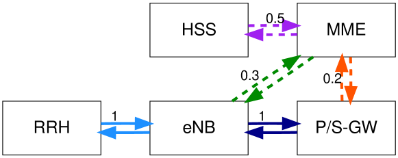
Figure 1: Logical graph for vEPC. Solid lines correspond to user traffic, dashed lines to control traffic.

The nature of 5G traffic further exacerbates this challenge. Indeed, as exemplified in Fig. 1, traffic flows in 5G need to traverse a logical graph whose vertices are VNFs; such graphs can have arbitrary complexity and are not restricted to being chains or directed acyclic graphs (DAGs). The task of the MANO entities can be described as matching such a logical graph with a physical graph whose vertices are B/F nodes and whose edges are the links, be them physical or virtual, that connect them. Such a matching must account for the fact that the quantity of traffic does not remain constant across processing steps (i.e., VNFs); in other words, the usual flow conservation laws do not hold.

Fig. 1, depicting the VNFs composing the virtual Evolved Packet Core (vEPC), depicts a typical example of this situation. Data-plane traffic flows from the remote radio head (RRH) to the eNodeB (eNB), and thence to the Packet/Service Gateway (P/S-GW). However, such a flow generate additional control-plane flows, e.g., going from the eNB to the Home Subscriber Server (HSS) through the Mobility Management Entity (MME). Even data traffic may not remain constant: as an example, firewalls and deep packet inspection (DPI) VNFs can drop some flows, thereby decreasing the network traffic from a processing step to the next.

Along with these challenges, the hybrid nature of 5G network nodes and their ability to be programmed through software results in significant opportunities, including the possibility to optimize the management of the network. Indeed, optimization is traditionally used in network design, but it is regarded to as too complex for their real-time management. In our work, we depart from this vision and integrate optimization within the MANO framework, thereby allowing its entities to make and implement high-quality and real-time decisions.

The main contributions of our paper are as follows:

• a model, capturing the unique features of 5G network nodes (e.g., their hybrid nature) and of the traffic they serve (e.g., no flow conservation);

• a problem formulation, allowing us to make joint decisions on (i) B/F node activation, (ii) number and placement of the VNF instances, and (iii) traffic routing;

• a solution concept, named OptiLoop, predicated on integrating optimization in the loop of the decisions made by MANO entities, namely the NFV orchestrator (NFVO);

• two implementations of OptiLoop, one within a real-world testbed based on OpenStack and OpenDaylight, and one within a larger-scale network emulated in Mininet.

The remainder of this paper is organized as follows. We review related work in Sec. II, and explain how our own work fits within the management and orchestration (MANO) framework proposed by ETSI in Sec. III. Next, we present our system model and problem formulation in Sec. IV, and detail the OptiLoop solution strategy in Sec. V. We then describe our testbeds’ architecture, reference scenario and benchmarks in Sec. VI, present numerical results in Sec. VII, and conclude the paper in Sec. VIII.

II Related work

Many works on VNF placement and traffic routing, including [1, 2, 3], take the approach of matching VNF and physical topology graphs, also proposing efficient solution strategies for the ensuing mixed-integer linear programming (MILP) problems. The optimization objectives are: minimizing network usage in [1], minimizing VNF deployment cost in [2], minimizing CAPEX and OPEX in [3]. The later work [4] takes an iterative approach, making VNF placement and routing decisions when a request arrives. [5] takes the VNF placement as given and focuses on scheduling and routing.

Other works focus on the interaction between mobile operators and third parties using their services. As an example, [6] considers a market where operators bid to serve incoming demands. Among energy-aware works, [7] seeks to optimize VNF placement and job scheduling in order to minimize energy consumption. However, the algorithm presented in [7] optimizes the server utilization but neglects the energy consumed by network elements such as B/F nodes.

Among the services that can be provided through SDN/NFV-based networks, a prominent example is the EPC. As suggested by the survey in [8], ILP and MILP are the most popular modeling tools, and heuristic algorithms the most popular solution strategy. A common theme [9, 10, 11] is splitting EPC elements, e.g., the Packet Gateway (P-GW) and Service Gateway (S-GW), into separate sub-elements, one dealing with control traffic and the other with user traffic. [12] finds that such an approach reduces the total cost of ownership. Interestingly, other works, e.g., [13, 14], take the opposite approach and merge P-GW and S-GW in a single entity (the P/S-GW). [13] focuses on the MME and proposes to implement it through four separate VNFs, whose number can vary so as to accommodate traffic fluctuations. Closer to our own effort is the recent work in [15], which studies the problem of placing the VNFs implementing the main EPC network functions – S-GW, P-GW and MME – across the available physical machines, subject to limits on their power and link capacity. A preliminary version [16] of this work addressed the same problem, albeit in simpler scenarios and with a more limited scope.

II-A Novelty

Our approach is novel with respect to the above works in several important ways:

1. first and foremost, the scope of our work: we jointly account for (i) the number and placement of VNF instances, (ii) traffic routing, and (iii) network management, e.g., activating/deactivating B/F nodes and links;

2. at the modeling level: accounting for the complexity of 5G traffic, with requests that originate at a network endpoint and traverse multiple VNFs, triggering additional requests as they do so (hence the quantity of traffic changes across processing steps);

3. as far as objectives are concerned: adopting energy-saving as our priority and using detailed and realistic energy models, instead of proxy metrics as in [7];

4. from a solution strategy viewpoint: optimizing in the loop, i.e., using optimization as a tool rather than a mere analysis technique;

5. at implementation level: validating and testing our approach through a testbed based on OpenDaylight and OpenStack.

III OptiLoop and the ETSI MANO framework

The management and orchestration (MANO) framework, standardized by ETSI in [17], includes a set of decision-making entities (functional blocks) in charge of managing NFV-based networks, along with the interfaces (reference points) between them. The high-level goal of the framework is to map the key performance indicators (KPIs) chosen by the verticals, e.g., maximum end-to-end latency, into decisions concerning the network resources, e.g., the activation/deactivation of (virtual) servers and the placement of VNFs therein. In the following, we present a short overview of the framework and then, in Sec. III-A, discuss the relationship between the NFV orchestrator, one of the most important MANO entities, and OptiLoop.

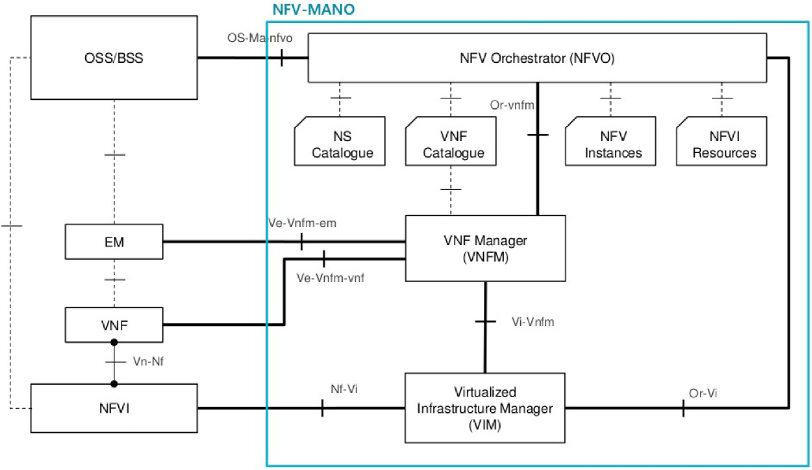
Figure 2: The NFV-MANO architectural framework. Source: [17]

Fig. 2, taken from [17], shows the decision-making entities of the MANO framework (within the blue area), along with the non-MANO entities they interact with. OSS/BSS (Operation and Business Support Services), at the top-left corner, are the contact point between verticals and mobile operators: they collect the vertical requirements, expressed through end-to-end KPIs, and convey them, through the Os-Ma-nfvo reference point, to the NFV Orchestrator (NFVO). The NFVO itself is arguably one of the most important entities of the MANO framework, and is in charge of the orchestration decisions. Specifically, given the vertical requirements and the state of the network infrastructure, the NFVO determines:

• how many instances of each VNF to deploy;

• where in the network infrastructure they shall run;

• the features of the virtual network connecting the VNF instances, e.g., the bandwidth of the links to traverse between them.

Through the Or-vnfm interface, these decisions are sent to the VNFM (VNF Manager), which takes care of instantiating the VNFs, requesting to the VIM (Virtual Infrastructure Manager) the needed resources, e.g., virtual machines or virtual links. The VIM, in turn, interacts with the NFVI (NFV Infrastructure), which includes the servers running the VNFs and the hypervisors managing them. The VNFM also communicates with a non-MANO entity called EM (Element Manager), in charge of FCAPS (Fault, Configuration, Accounting, Performance and Security) management, in order to configure the VNFs or collect/monitor KPIs from them.

III-A The NFVO: input, output, and decisions

The NFVO is in charge of most of the orchestration tasks in the MANO framework. Owing to its importance, in the following we detail the decisions it is in charge of, along with the input information it has access to; such pieces of information correspond, respectively, to the output and input of OptiLoop.

The main input data used by the NFVO is the NSD (Network Service Descriptor), a data structure defined in [17, Sec. 6.2.1]. NSDs contain a graph description of the VNFs needed by each service, called VNFFG (VNF Forwarding Graph) [17, Sec. 6.5.1] along with deployment flavor information, including the maximum latency acceptable for each service[17, Sec. 6.2.1.3]. Furthermore, the NFVO has access to information on the network infrastructure, e.g., the state and capabilities of network and computing resources available at the NFV infrastructure, including details about the connectivity among the servers where the VNFs will be allocated.

Using all the above, the NFVO makes decisions about:

• the status of network infrastructure elements, e.g., servers;

• VNF lifecycle management [17, Sec. 7.2] about the VNFs, including the host they run at;

• routing, accounting for the capacity and delay of virtual links.

Such decisions will correspond to decision variables in our system model, as detailed next.

IV System model

Our model is based on two graphs, a logical one and a physical one. For simplicity, we describe it with reference to unidirectional traffic; notice however that our model and our results also account for bidirectional traffic. Tab. I summarizes all the notation we introduce below.

IV-A The logical graph

The logical graph, exemplified in Fig. 1, describes where, i.e., which endpoint, the traffic comes from, and how it is processed. Its vertices are either endpoints $e\in\mathcal{E}$ or VNFs $v\in\mathcal{V}$. With reference to Fig. 1, we have $\mathcal{E}=\{\text{RRH}\}$, and $\mathcal{V}=\{\text{eNB},\text{P/S-GW},\text{MME},\text{HSS}\}$.

On the logical graph, we have logical flows $l(e,v_{1},v_{2})$ representing data originating from endpoint $e$ and going from VNF $v_{1}$ to VNF $v_{2}$. Additionally, with an abuse of notation, we indicate with $l(e,v)$ flows that start from endpoint $e$ and are first processed at VNF $v$, e.g., from the RRH to the eNB in Fig. 1. Note that keeping track of the endpoint at which flows originate, i.e., having an $e$ index in our variables, serves a manifold purpose. First, it allows our model to account for the fact that different types of traffic (i.e., originating from different endpoints) may need different processing, i.e., traverse different VNF graphs. Furthermore, such VNF graphs may overlap; in this case, keeping track of the origin of the flows makes it possible to distinguish them even if they traverse the same VNF. Finally, it allows routing each flow in a different way, in both the logical and the physical graph. Notice that different traffic flows coming from the same physical endpoint can be distinguished by associating them to different logical endpoints.

Another important aspect of the system is that there is no flow conservation in the logical graph. As an example, in Fig. 1 we see a user flow of $1$ traffic unit going from the RRH to eNB and thence to the gateway, which triggers some additional control traffic from the eNB and the gateway to the MME. Indeed, the following generalized flow conservation law holds for each endpoint $e$ and VNFs $v_{2},v_{3}$:

$$l(e,v_{2},v_{3}){=}\sum_{v_{1}\in\mathcal{V}}l(e,v_{1},v_{2})\chi(v_{1},v_{2},v_{3})+l(e,v_{2})\chi(e,v_{2},v_{3}).$$

The above expression represents the logical flow originated at endpoint $e$, outgoing from VNF $v_{2}$ and directed to VNF $v_{3}$. Such a quantity is equal to the sum between logical flows entering $v_{2}$, from either a VNF $v_{1}$ or the endpoint $e$ itself, multiplied by a factor $\chi$. In particular, $\chi(v_{1},v_{2},v_{3})$ is used to quantify the amount of logical flow directed to $v_{3}$ that is generated when traffic coming from $v_{1}$ is processed at VNF $v_{2}$. With reference to the eNB in Fig. 1, we have $\chi(\text{RRH},\text{eNB},\text{P/S-GW})=1$, while $\chi(\text{RRH},\text{eNB},\text{MME})=0.3$. Similarly, for the gateway, we have $\chi(\text{eNB},\text{P/S-GW},\text{MME})=0.2$. At the MME we have flow conservation, i.e., $\chi(\text{eNB},\text{MME},\text{HSS})=\chi(\text{P/S-GW},\text{MME},\text{HSS})=1$. In $\chi(e,v_{2},v_{3})$, we abuse the notation and allow the first index of $\chi$ to be an endpoint instead of a VNF. We remark that $\chi$-values lower than one can also represent, e.g., a firewall dropping some of the incoming traffic. Also notice that $\chi$-values different from one can happen for both control traffic (e.g., the eNB in Fig. 1) and user traffic (as in the case of the firewall).

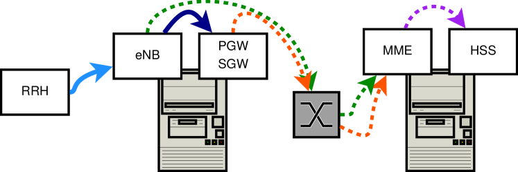
Figure 3: Example implementation of the logical graph in Fig. 1 over a physical network. Each line corresponds to a physical flow, i.e., to a $\tau$-variable; their color and style match the logical flows in Fig. 1.

IV-B The physical graph

In the physical graph, vertices correspond to the endpoints $e\in\mathcal{E}$ and the B/F nodes $c\in\mathcal{C}$. In general, B/F nodes have computational capabilities $k(c)$; B/F nodes that cannot host any VNF (e.g., switches) have $k(c)=0$. Fig. 3 presents a possible implementation of the logical VNF graph in Fig. 1, where VNFs are placed on each of the two B/F nodes with processing capabilities. For simplicity, we present our model with reference to the case where multiple VNF instances can be deployed across different nodes, but at most one instance of each VNF can be deployed at each B/F node.

Traffic traversing link $(i,j)\in\mathcal{L}\subseteq(\mathcal{C}\cup\mathcal{E})^{2}$ is also subject to a network delay $D_{i,j}$. Such a delay is static, i.e., every unit of traffic traversing link $(i,j)$ incurs a delay $D_{i,j}$. Furthermore, links $(i,j)$ have a bandwidth $B_{i,j}$, corresponding to the maximum amount of traffic that can go from B/F node $i$ to B/F node $j$ without generating congestion.

Our main variable is represented by physical flows $\tau_{i,j}(e,v_{1},v_{2})$, representing the amount of traffic that was originated from endpoint $e$, last visited VNF $v_{1}$, will next visit VNF $v_{2}$, and is now traveling on link $(i,j)$. Recall that we have to keep track of the flow originating endopint, in order to model traffic routing. If the flow has never been processed, i.e., it is going from $e\in\mathcal{E}$ to its first VNF $v\in\mathcal{V}$, we will conventionally set $v_{1}=v_{2}=v$ and write $\tau_{i,j}(e,v,v)$.

Given a B/F node $c\in\mathcal{C}$, we denote by $t_{c}(e,v_{1},v_{2})$ the amount of traffic that is just transiting by $c$ (i.e., it is not processed at $c$) and it was originated at $e$, last visited VNF $v_{1}$ and will next visit VNF $v_{2}$. Similarly, $p_{c}(e,v_{1},v_{2})$ is the traffic that is processed at B/F node $c$, it was originated at $e$, and last visited VNF $v_{1}$. Note that $p_{c}(e,v_{1},v_{2})>0$ implies that an instance of VNF $v_{2}$ is deployed at $c$.

Traffic being processed at VNF $v$ is subject to a delay $D(v)$. Normally, processing delay is linked to the amount of resources (e.g., CPU) allocated to each VNF, and such an amount depends on the other VNFs deployed at the same B/F node. In our case, however, energy is the main metric of interest, and we can therefore assume that no VNF will be allocated more resources than the minimum amount required by the VNF itself.

A first constraint we need to impose is that, given a generic VNF $v_{2}$, the traffic originated at $e$, that has been processed through VNF $v_{1}$ and is entering B/F node $c$, is either (i) processed at an instance of $v_{2}$ located in $c$, or (ii) transiting by $c$ while being routed toward an instance of $v_{2}$. Thus, for any $c,e,v_{1},v_{2}$, we have:

$$\sum_{(i,c)\in\mathcal{L}}\tau_{i,c}(e,v_{1},v_{2})=t_{c}(e,v_{1},v_{2})+p_{c}(e,v_{1},v_{2}).$$ (1)

A similar constraint concerns the traffic outgoing from $c$. For any $c$, endpoint $e$ and VNFs $v_{2},v_{3}$, we have:

$$\sum_{(c,j)\in\mathcal{L}}\tau_{c,j}(e,v_{2},v_{3}){=}t_{c}(e,v_{2},v_{3})\mathord{+}\sum_{v_{1}\in\mathcal{V}}p_{c}(e,v_{1},v_{2})\chi(v_{1},v_{2},v_{3})$$ (2)

where $v_{2}$ is the last VNF that traffic visited, either before arriving at $c$ (if traffic just transits by $c$) or at $c$ itself (if $v_{2}$ is deployed therein, i.e., $p_{c}(e,v_{1},v_{2})>0$). $v_{3}$ instead is the VNF that traffic will visit next. In other words, (1)–(2) enforce ordinary flow conservation for the traffic that is transiting at $c$, i.e., using $c$ as a traditional switch, and generalized flow conservation for the traffic that is processed at $c$.

Next, we need to ensure that we only use active B/F nodes and links, and their capacity is not exceeded. We define two sets of binary variables, $x_{i,j}$ and $y_{c}$, indicating whether link $(i,j)$ and B/F node $c$ are active or not.

For links, we need to impose:

$$x_{i,j}\leq\min\left\{y_{i},y_{j}\right\},\quad\forall(i,j)\in\mathcal{L}\,,$$ (3)

i.e., no link can be active if either of its ends is off, and

$$\sum_{e\in\mathcal{E}}\sum_{v_{1},v_{2}\in\mathcal{V}}\tau_{i,j}(e,v_{1},v_{2})\leq x_{i,j}B_{i,j},\quad\forall(i,j)\in\mathcal{L}.$$ (4)

TABLE I: Notation

Symbol	Type	Meaning
$\mathcal{E}$	Set	Set of network endpoints
$\mathcal{C}$	Set	Set of B/F nodes
$\mathcal{L}$	Set	Set of links
$\mathcal{V}$	Set	Set of VNFs
$B_{i,j}$	Parameter	Bandwidth of link $(i,j)\in\mathcal{L}$
$D_{i,j}$	Parameter	Delay of link $(i,j)\in\mathcal{L}$
$\chi(v_{1},v_{2},v_{3})$	Parameter	How much traffic resulting from the processing at VNF $v_{2}$, which was previously processed at VNF $v_{1}$, is meant to be next processed at VNF $v_{3}$
$\delta(c,v)$	Binary var.	Whether we deploy VNF $v\in\mathcal{V}$ at B/F node $c\in\mathcal{C}$
$f_{0}$	Function	Energy consumption due to placing a VNF at a B/F node
$f_{\text{idle}}$	Function	Energy consumption due to activating a B/F node
$f_{\text{proc}}$	Function	Traffic-dependent energy consumption due to processing
$f_{\text{sw}}$, $f_{\text{link}}$	Function	Traffic-dependent energy consumption at switches and links
$k(c)$	Parameter	Computational capability of B/F node $c\in\mathcal{C}$
$l(e,v_{1},v_{2})$	Parameter	Logical flow originated at $e\in\mathcal{E}$ and going from VNF $v_{1}\in\mathcal{V}$ to VNF $v_{2}\in\mathcal{V}$
$l(e,v)$	Parameter	Logical flow originating at $e\in\mathcal{E}$ and first being processed at VNF $v\in\mathcal{V}$
$p_{c}(e,v_{1},v_{2})$	Continuous var.	How much traffic coming from users connected to endpoint $e\in\mathcal{E}$ for service that was last processed at VNF $v_{1}$ is processed by an instance of VNF $v_{2}$ deployed at B/F node $c$
$r(v)$	Parameter	Computational capability required to process one traffic unit of VNF $v\in\mathcal{V}$
$\rho(c)$	Parameter	Computational capability consumed by one unit of traffic transiting by B/F node (SW switch) $c\in\mathcal{C}$
$\tau_{i,j}(e,v_{1},v_{2})$	Continuous var.	How much traffic coming from users connected to endpoint $e\in\mathcal{E}$ that was last processed at VNF $v_{1}$ and meant to be next processed at VNF $v_{2}$ goes through link $(i,j)\in\mathcal{L}$
$t_{c}(e,v_{1},v_{2})$	Continuous var.	How much traffic originating from $e$ that was last processed at VNF $v_{1}$ and meant to be next processed at VNF $v_{2}$ transits (without processing) by B/F node $c\in\mathcal{C}$
$x_{i,j}$	Binary var.	Whether link $(i,j)\in\mathcal{L}$ is active
$y_{c}$	Binary var.	Whether B/F node $c\in\mathcal{C}$ is active

With regard to processing, inactive B/F nodes cannot host any VNF. We track this through a binary variable $\delta(c,v)$ expressing whether an instance of VNF $v$ is deployed at B/F node $c$, and impose:

$$\delta(c,v)\leq y_{c},\quad\forall c\in\mathcal{C},v\in\mathcal{V}.$$ (5)

Additionally, no processing can be done for VNFs that are not deployed at a given B/F node:

$$p_{c}(e,v_{1},v_{2})\leq\delta(c,v_{2})k(c),\quad\forall c\in\mathcal{C},e\in\mathcal{E},v_{1},v_{2}\in\mathcal{V}.$$ (6)

Finally, each traffic unit processed by VNF $v$ requires $r(v)$ computational capability, and, assuming $c$ is a software switch, each unit of traffic switched by $c$ consumes $\rho(c)$ CPU. Clearly, the computational capability of each B/F node $c$ must be sufficient for both, i.e., for any B/F node $c$,

$$\sum_{e\in\mathcal{E}}\sum_{v_{1}\in\mathcal{V}}\sum_{v_{2}\in\mathcal{V}}\Bigg{[}r(v_{2})p_{c}(e,v_{1},v_{2})+\\ +\rho(c)\sum_{(c,j)\in\mathcal{L}}\tau_{c,j}(e,v_{1},v_{2})\Bigg{]}\leq k(c),$$ (7)

where $\rho(c)$ multiplies the total traffic outgoing from $c$.

Next, we ensure that the delay of the traffic originated at any endpoint $e$ does not exceed a threshold $D^{\max}(e)$:

$$\frac{\sum_{i,j\in\mathcal{L}}\sum_{v_{1},v_{2}\in\mathcal{V}}D_{i,j}\tau_{i,j}(e,v_{1},v_{2})}{\sum_{v\in\mathcal{V}}l(e,v)}+\\ +\frac{\sum_{v_{1},v_{2}\in\mathcal{V}}\sum_{c\in\mathcal{C}}D(v_{2})p_{c}(e,v_{1},v_{2})}{\sum_{v\in\mathcal{V}}l(e,v)}\leq D^{\max}(e).$$ (8)

The two terms on the left hand side of (8) correspond to the network and processing delay, respectively. The first term of (8) is a summation of terms in the form $D_{i,j}\frac{\tau_{i,j}}{l}$, each representing the delay incurred by traversing link $(i,j)$ weighted by the fraction of traffic traversing it. Similarly, the second term of (8) is a summation of terms in the form $D(v)\frac{p_{c}}{l(e,v)}$, weighting the processing delay of VNF $v$ by the fraction of traffic processed by it.

At last, logical and physical flows have to match. To this end, it is sufficient to impose that, for each logical flow $l(e,v)$ going from endpoint $e$ to VNF $v$, there are corresponding physical flows of the type $\tau_{e,j}(e,v,v)$, such that:

$$l(e,v)=\sum_{(e,j)\in\mathcal{L}}\tau_{e,j}(e,v,v),\quad\forall e\in\mathcal{E},v\in\mathcal{V}.$$ (9)

Eq. (9) ensures that the traffic injected from endpoints to B/F nodes on the physical graph matches the logical traffic going from endpoints to VNFs. Thanks to the flow conservation constraints (1)–(2), this also implies that such traffic is processed and transformed as dictated by the $\chi$-parameters, i.e., that all physical flows match their logical counterpart.

IV-C Energy and objective

There are five contributions to the overall energy consumption we are interested in tracking:

• activating a B/F node, resulting in a consumption of $f_{\text{idle}}$;

• placing a VNF on a B/F node, resulting in a consumption $f_{0}$ due to, e.g., virtual machines overhead;

• using said VNF, resulting in a consumption of $f_{\text{proc}}$ depending on the computational resources used;

• switching traffic at a B/F node, resulting in a consumption of $f_{\text{sw}}$ depending on the traffic switched by the node;

• having traffic going through links, resulting in a consumption of $f_{\text{link}}$ depending on the traffic over each link.

The corresponding energy consumption is:

$$E_{\text{idle}}=\sum_{c\in\mathcal{C}}f_{\text{idle}}\left(y_{c}\right);\quad\quad E_{0}=\sum_{c\in\mathcal{C}}\sum_{v_{2}\in\mathcal{V}}f_{0}\left(\delta(c,v_{2})\right);$$

$$E_{\text{proc}}=\sum_{c\in\mathcal{C}}f_{\text{proc}}\left(\sum_{v_{2}\in\mathcal{V}}r(v)\sum_{e\in\mathcal{E}}\sum_{v_{1}\in\mathcal{V}}p_{c}(e,v_{1},v_{2})\right);$$

$$E_{\text{sw}}=\sum_{c\in\mathcal{C}}f_{\text{sw}}\left(\sum_{e\in\mathcal{E}}\sum_{v_{1},v_{2}\in\mathcal{V}}\tau_{c,j}(e,v_{1},v_{2})\right);$$

$$E_{\text{link}}=\sum_{(i,j)\in\mathcal{L}}f_{\text{link}}\left(\sum_{e\in\mathcal{E}}\sum_{v_{1},v_{2}\in\mathcal{V}}\tau_{i,j}(e,v_{1},v_{2})\right).$$

Given all this, our objective can be written as:

$$\min_{x,y}E=E_{0}+E_{\text{proc}}+E_{\text{idle}}+E_{\text{sw}}+E_{\text{link}},$$ (10)

subject to the following constraints:

$$l(e,v_{2},v_{3}){=}\sum_{v_{1}\in\mathcal{V}}l(e,v_{1},v_{2})\chi(v_{1},v_{2},v_{3})+l(e,v_{2})\chi(e,v_{2},v_{3})$$

$$\sum_{(i,c)\in\mathcal{L}}\tau_{i,c}(e,v_{1},v_{2})=t_{c}(e,v_{1},v_{2})+p_{c}(e,v_{1},v_{2})$$

$$\sum_{(c,j)\in\mathcal{L}}\tau_{c,j}(e,v_{2},v_{3}){=}t_{c}(e,v_{2},v_{3})\mathord{+}\sum_{v_{1}\in\mathcal{V}}p_{c}(e,v_{1},v_{2})\chi(v_{1},v_{2},v_{3})$$

$$\sum_{e\in\mathcal{E}}\sum_{v_{1},v_{2}\in\mathcal{V}}\tau_{i,j}(e,v_{1},v_{2})\leq x_{i,j}B_{i,j}$$

$$\delta(c,v)\leq y_{c}\quad;\quad l(e,v)=\sum_{(e,j)\in\mathcal{L}}\tau_{e,j}(e,v,v)$$

$$p_{c}(e,v_{1},v_{2})\leq\delta(c,v_{2})k(c)\quad;\quad x_{i,j}\leq\min\left\{y_{i},y_{j}\right\}$$

$$\sum_{e\in\mathcal{E}}\sum_{v_{1}\in\mathcal{V}}\sum_{v_{2}\in\mathcal{V}}\left[r(v_{2})p_{c}(e,v_{1},v_{2}){+}\rho(c)\sum_{(c,j)\in\mathcal{L}}\tau_{c,j}(e,v_{1},v_{2})\right]{\leq}k(c)$$

$$\frac{\sum_{i,j\in\mathcal{L}}\sum_{v_{1},v_{2}\in\mathcal{V}}D_{i,j}\tau_{i,j}(e,v_{1},v_{2})}{\sum_{v\in\mathcal{V}}l(e,v)}+\\ +\frac{\sum_{v_{1},v_{2}\in\mathcal{V}}\sum_{c\in\mathcal{C}}D(v_{2})p_{c}(e,v_{1},v_{2})}{\sum_{v\in\mathcal{V}}l(e,v)}\leq D^{\max}(e)$$ (11)

IV-D Multiple VNF instances

So far, we have presented our problem formulation with reference to the case that at most one instance of each VNF can be placed at each B/F node. This is true in many cases; however, there are situations (e.g., coexisting services with isolation requirements) when we may need to place multiple instances of the same VNF at the same B/F node. In the following, we extend our model to describe such a case.

To begin with, we need to distinguish VNFs from VNF instances. To this end, we introduce a new set $\mathcal{W}=\{w\}$ representing the VNF instances, and indicate as $V(w)\in\mathcal{V}$ the type of instance $w$, i.e., the VNF $w$ is an instance of.

Furthermore, we need to account for the fact that logical flows happen between VNFs, while physical flows happen between VNF instances and processing takes place at VNF instances. Therefore, we need to replace:

• $\tau_{i,c}(e,v_{1},v_{2})$ with $\tau_{i,c}(e,w_{1},w_{2})$, where $w_{1},w_{2}\in\mathcal{W}$;

• $t_{c}(e,v_{1},v_{2})$ with $=t_{c}(e,w_{1},w_{2})$;

• $p_{c}(e,v_{1},v_{2})$ with $=p_{c}(e,w_{1},w_{2})$.

In order to guarantee that physical and logical flows match, we also need to replace (9) with:

$$l(e,v)=\sum_{(e,j)\in\mathcal{L}}\sum_{w\in\mathcal{W}:V(w)=v}\tau_{e,j}(e,w,w),\quad\forall e\in\mathcal{E},v\in\mathcal{V},$$ (12)

where, in (12), the second summation accounts for all instances $w$ of VNF $v$.

Finally, (2) needs to be changed in order to represent the fact that that data can flow from any instance of a VNF to any instance of the next VNF in the logical graph:

$$\sum_{(c,j)\in\mathcal{L}}\sum_{\begin{subarray}{c}w_{2},w_{3}\in\mathcal{W}\colon\\ V(w_{2})=v_{2}\\ V(w_{3})=v_{3}\end{subarray}}\tau_{c,j}(e,w_{2},w_{3})=\sum_{\begin{subarray}{c}w_{2},w_{3}\in\mathcal{W}\colon\\ V(w_{2})=v_{2}\\ V(w_{3})=v_{3}\end{subarray}}t_{c}(e,w_{2},w_{3})+\\ +\sum_{\begin{subarray}{c}w_{1}\in\mathcal{W}\colon\\ V(w_{1})=v_{1}\end{subarray}}\sum_{\begin{subarray}{c}w_{2},w_{3}\in\mathcal{W}\colon\\ V(w_{2})=v_{2}\\ V(w_{3})=v_{3}\end{subarray}}p_{c}(e,w_{1},w_{2})\chi(v_{1},v_{2},v_{3}).$$ (13)

In (13), notice how the $\chi$-variable, which concerns logical flows, has as its indices VNFs in $\mathcal{V}$, while the $\tau$- and $p$-variables have as indices VNF instances in $\mathcal{W}$.

V The OptiLoop strategy

The problem stated in Sec. IV falls into the MILP category, and is thus impractical to solve in real time. We can however solve its relaxed version, where binary variables are allowed to take any value in $[0,1]$. Optimal solutions to the relaxed models cannot be directly used to manage (or plan) a network; however, they can provide useful guidelines.

Figure 4: The OptiLoop strategy. We begin by obtaining an initial feasible solution, as described in Sec. V-A. After that, we periodically check the current solution for problems (procedure fixProblems, described in Alg. 1) and for opportunities to deactivate some B/F nodes and/or links (procedure saveEnergy, described in Alg. 2).

Our basic idea of is to leverage the software-defined nature of our network to make an optimizer interact with SDN controllers and NFVOs, i.e., optimize problems as a part of our network management strategy. Our solution strategy is called OptiLoop (for Optimization in the Loop) and it includes the following steps, as outlined in Fig. 4: (i) we initialize the system with a feasible (albeit potentially suboptimal) solution, as detailed in Sec. V-A; (ii) after that, we periodically:

1. check that the network configuration is adequate to the current (and/or predicted) demand;

2. if not so, activate additional VNFs, B/F nodes, and/or links as needed;

3. check whether there are B/F nodes and/or links that can be deactivated in order to save energy;

4. if so, update the current network configuration accordingly.

Sec. V-A explains how we obtain the initial solution, i.e., Item (i) above. Items (1)–(2) and (3)–(4) correspond to the fixProblems and saveEnergy procedures respectively, which are described in Sec. V-B and Sec. V-C.

It is worth pointing out that the fixProblems and saveEnergy procedures are designed to take no action if no action is warranted, and therefore there is no harm in cascading them. As an example, fixProblems will never take any action the first time it is executed after an initial solution is generated, as that solution is guaranteed to be feasible. Similarly, saveEnergy is unlikely to find elements to deactivate if fixProblems just had to activate some.

V-A Initial solution

The initial solution used to initialize OptiLoop has to be feasible, but does not have to be optimal. It can come from one of the heuristics we reviewed in Sec. II, or it can be obtained by solving a version of our problem where:

1. all B/F nodes and links are active, i.e., $y_{c}=1,\forall c\in\mathcal{C}$ and $x_{i,j}=1,\forall(i,j)\in\mathcal{L}$;

2. there is an instance of all VNFs deployed at each B/F node, i.e., $\delta(c,v)=1,\forall c\in\mathcal{C},v\in\mathcal{V}$.

The resulting solution will be highly suboptimal, as we are likely to needlessly activate B/F nodes and/or links and to place useless VNF instances, all of which increase the power consumption. On the plus side, the problem is LP, as all binary variables are fixed; furthermore, the following property holds.

Property 1

If a problem instance is feasible, then there is at least one feasible solution where the $x,y$ and $\delta$ variables are all set to $1$.

Proof:

Let us consider a feasible solution $\mathcal{S}^{0}$, where some of the binary variables are set to zero and others to one. By hypothesis, $\mathcal{S}^{0}$ is feasible. What we need to prove is that changing all binary variables to one can never make us violate a constraint. This follows by inspection of (3), (4), (5), (6): if they hold for the variable values in $\mathcal{S}^{0}$, then they will also hold when all binary variables are set to one. ∎

In other words, setting all binary variables to one is an easy way to obtain a feasible solution to our problem to start with. This solution can be vastly improved, as discussed next.

V-B The fixProblems procedure

The high-level goal of the fixProblems procedure is to check whether the current network configuration can cope with the current (and projected) traffic demand. If this is not the case, then we take one or more of the following actions: (i) activating additional B/F nodes; (ii) activating additional links; (iii) deploying additional VNF instances.

Specifically, as detailed in Alg. 1, we take as an input the current solution $\mathcal{S}^{\text{curr}}$. We then proceed, in Line 2–Line 5, to create a new instance $\mathcal{P}$ of the problem, where all binary variables are fixed to their values in $\mathcal{S}^{\text{curr}}$. In Line 6, we solve such a problem: if it is feasible, then no action is required and the algorithm exits (Line 8). Otherwise, we look at why the problem is infeasible, by inspecting its irreducible inconsistent subsystem (IIS), i.e., the subset of constraints such that removing any of them would make the problem feasible. This set allows us to discriminate between the different reasons that can make the network unable to operate properly (hence, the problem infeasible).

Algorithm 1 The fixProblems procedure.

1:$\mathcal{S}^{\text{curr}}$

2:$\mathcal{P}\leftarrow\textbf{new}\text{ problem}()$

3:$\mathcal{P}.\text{fix}(x_{i,j}\leftarrow x^{\text{curr}}_{i,j},\quad\forall(i,j)\in\mathcal{L})$

4:$\mathcal{P}.\text{fix}(y_{c}\leftarrow y^{\text{curr}}_{c},\quad\forall c\in\mathcal{C})$

5:$\mathcal{P}.\text{fix}(\delta(c,v)\leftarrow\delta^{\text{curr}}(c,v),\quad\forall c\in\mathcal{C},v\in\mathcal{V})$

6:$\textbf{solve}(\mathcal{P})$

7:if $\mathcal{P}.\text{is\_feasible}$ then

8:     return

9:if (4)$\in\mathcal{P}.\text{IIS}$ then

10:     $\mathcal{P}.\text{relax}(x_{i,j}\colon x^{\text{curr}}_{i,j}=0)$

11:     $\mathcal{P}.\text{relax}(y_{c}\colon y^{\text{curr}}_{c}=0)$

12:     $\tilde{x},\tilde{y}\leftarrow\textbf{solve}(\mathcal{P})$

13:     $(i^{\star},j^{\star}){\leftarrow}\textbf{choose}\text{ from }\mathcal{L}\text{ with prob. }\tilde{x}_{i,j}$

14:     $\mathcal{P}.\text{fix}(x_{i^{\star},j^{\star}}\leftarrow 1)$

15:     $\mathcal{P}.\text{fix}(y_{i}\leftarrow 1;y_{j}\leftarrow 1)$

16:     goto Line 6

17:if (7)$\in\mathcal{P}.\text{IIS}$ then

18:     $\mathcal{P}.\text{relax}(y(c)\colon y^{\text{curr}}(c)=0)$

19:     $\mathcal{P}.\text{relax}(\delta(c,v)\colon\delta^{\text{curr}}(c,v)=0)$

20:     $\tilde{\delta}\leftarrow\textbf{solve}(\mathcal{P})$

21:     $c^{\star},v^{\star}{\leftarrow}\textbf{choose}\text{ from }\mathcal{C}\times\mathcal{V}\text{ with prob. }\tilde{\delta}(c,v)$

22:     $\mathcal{P}.\text{fix}(y(c^{\star})\leftarrow 1)$

23:     $\mathcal{P}.\text{fix}(\delta(c^{\star},v^{\star})\leftarrow 1)$

24:     goto Line 6

If constraint (4) (mandating that no link is used for more than its capacity) is in the IIS, then we need to activate some more links and/or B/F nodes. To decide which ones, we relax all $x$- and $y$-variables related to B/F nodes and links that were inactive in $\mathcal{S}^{\text{curr}}$ (Line 10–Line 11) and solve the new problem (Line 12). We then choose one link to activate, with a probability proportional to its relaxed $\tilde{x}_{i,j}$ value, and fix to 1 the corresponding $x$-value and the $y$-values of its endpoints (Line 13–Line 15). We then go back to Line 6 and test the new solution (Line 16). If it is still infeasible, we will activate further network elements until feasibility is achieved.

We proceed in a similar way if constraint (7) is in the IIS, i.e., if we have a computational capability issue. We relax variables $y$ and $\delta$, allowing for more B/F nodes to be activated and VNFs to be deployed if needed, and solve the new problem obtaining the relaxed values $\tilde{\delta}$ (Line 18–Line 20). We then have to decide which VNF to place and where. We do so by selecting a B/F node $c^{\star}$ and a VNF $v^{\star}$ at random, with a probability proportional to the relaxed values $\tilde{\delta}(c,v)$, and fix the corresponding $y$ and $\delta$-variable to $1$ (Line 21–Line 23). Finally, we go back to testing the new solution (Line 24).

Note that all problems we solve in Alg. 1 are LP: in Line 6, Line 12 and Line 20 all binary variables are either fixed or relaxed. Such problems can be therefore solved in polynomial time (embedded [18] optimization on low-power hardware is now commonplace in several application domains).

V-C The saveEnergy procedure

We can think of the saveEnergy procedure as the dual of fixProblems. Our aim is to identify B/F nodes and/or links that can be deactivated, as well as VNF instances that can be removed from the B/F nodes they run into. The objective is to reduce our power consumption without impairing our ability to serve the traffic, i.e., without making the problem infeasible. As in the fixProblems procedure, we solve a sequence of LP problems with fixed or relaxed variables, obtaining guidance on the decisions we should make and their effects.

In Alg. 2, we take the current solution $\mathcal{S}^{\text{curr}}$ as an input. We then create an instance $\mathcal{P}$ of the problem where the binary variables that in the current solution have value 0 are fixed to 0 (Line 3–Line 5), and those that have currently value 1 are relaxed (Line 6–Line 8). This is because we are not looking for new nodes/links to activate, but for elements to deactivate. We do so by solving the problem instance $\mathcal{P}$ (Line 9); note that all binary variables therein are fixed or relaxed, so the problem is LP.

Algorithm 2 The saveEnergy procedure.

1:$\mathcal{S}^{\text{curr}}$

2:$\mathcal{P}\leftarrow\textbf{new}\text{ problem}()$

3:$\mathcal{P}.\text{fix}(x_{i,j}\leftarrow 0,\quad\forall(i,j)\in\mathcal{L}\colon x^{\text{curr}}_{i,j}=0)$

4:$\mathcal{P}.\text{fix}(y_{c}\leftarrow 0,\quad\forall c\in\mathcal{C}\colon y^{\text{curr}}_{c}=0)$

5:$\mathcal{P}.\text{fix}(\delta(c,v)\leftarrow 0,\quad\forall c\in\mathcal{C},v\in\mathcal{V}\colon\delta(c,v)=0)$

6:$\mathcal{P}.\text{relax}(x_{i,j},\quad\forall(i,j)\in\mathcal{L}\colon x^{\text{curr}}_{i,j}=1)$

7:$\mathcal{P}.\text{relax}(y_{c},\quad\forall c\in\mathcal{C}\colon y^{\text{curr}}_{c}=1)$

8:$\mathcal{P}.\text{relax}(\delta(c,v),\quad\forall c\in\mathcal{C},v\in\mathcal{V}\colon\delta(c,v)=1)$

9:$\textbf{solve}(\mathcal{P})$

10:$(x^{\star},y^{\star})\leftarrow\arg\min_{(x,y)\in\mathcal{L}\colon x_{x,y}^{\text{curr}}=1}\tilde{x}_{i,j}$

11:$c^{\star}\leftarrow\arg\min_{c\in\mathcal{C}\colon y^{\text{curr}}(c)=1}\tilde{y}(c)$

12:$d^{\star},v^{\star}\leftarrow\arg\min_{c,v\in\mathcal{C}\times\mathcal{V}\colon\delta^{\text{curr}}(c,v)=1}\tilde{\delta}(c,v)$

13:$\mathcal{P}_{2}\leftarrow\textbf{copy}(\mathcal{P})$

14:if $\tilde{x}_{i^{\star},j^{\star}}<\tilde{y}(c^{\star})\wedge\tilde{x}_{i^{\star},j^{\star}}<\tilde{\delta}(d^{\star},v^{\star})$ then

15:     $\mathcal{P}_{2}.\text{fix}(x_{i^{\star},j^{\star}}\leftarrow 0)$

16:if $\tilde{y}(c^{\star})<\tilde{x}_{i^{\star},j^{\star}}\wedge\tilde{y}(c^{\star})<\tilde{\delta}(d^{\star},v^{\star})$ then

17:     $\mathcal{P}_{2}.\text{fix}(y(c^{\star})\leftarrow 0)$

18:     $\mathcal{P}_{2}.\text{fix}(x_{i,j}\leftarrow 0,\quad\forall(i,j)\in\mathcal{L}\colon i=c^{\star}\vee j=c^{\star}$)

19:     $\mathcal{P}_{2}.\text{fix}(\delta(c,v)\leftarrow 0,\quad\forall c\in\mathcal{C},v\in\mathcal{V}\colon c=c^{\star}$)

20:if $\tilde{\delta}(d^{\star},v^{\star})<\tilde{x}_{i^{\star},j^{\star}}\wedge\tilde{\delta}(d^{\star},v^{\star})<\tilde{y}(c^{\star})$ then

21:     $\mathcal{P}_{2}.\text{fix}(\delta(d^{\star},v^{\star})\leftarrow 0)$

22:$\textbf{solve}(\mathcal{P}_{2})$

23:if $\mathcal{P}_{2}.\text{is\_feasible}$ then

24:     $\mathcal{P}\leftarrow\mathcal{P}_{2}$

25:     goto Line 2

26:else

27:     return $\mathcal{P}$

In Line 10–Line 12 we identify the link, B/F node, and pair of B/F node and VNF that are active in the current solution and have the lowest value of the associated relaxed variable (respectively $\tilde{x}_{i,j}$, $\tilde{y}(c)$, and $\tilde{\delta}(c,v)$). Intuitively, these are the elements that most likely can be deactivated without impairing network functionality. We check this by creating a copy of problem instance $\mathcal{P}$ and fixing to $0$ the binary variable associated to the element with the lowest value of the relaxed variables (Line 13–Line 21). If that element is a B/F node, we also need to deactivate the links using it and the VNF instances it hosts (Line 18–Line 19).

The difference between $\mathcal{P}$ and $\mathcal{P}_{2}$ is that exactly one element that was active in $\mathcal{P}$ is deactivated in $\mathcal{P}_{2}$, hence $\mathcal{P}_{2}$ is also LP. In Line 22, we solve $\mathcal{P}_{2}$ and check if it is feasible. If that is the case, then we use $\mathcal{P}_{2}$ as our new solution, and try to further enhance it (Line 24–Line 25). Otherwise, the algorithm returns $\mathcal{P}$, the last feasible solution we tried.

In summary, Alg. 2 deactivates zero or more elements, i.e., B/F nodes, links, or VNF instances. The element to deactivate is chosen based on the value taken by the corresponding relaxed variable, and after each change we check that the resulting configuration can serve its load, i.e., the problem instance is feasible.

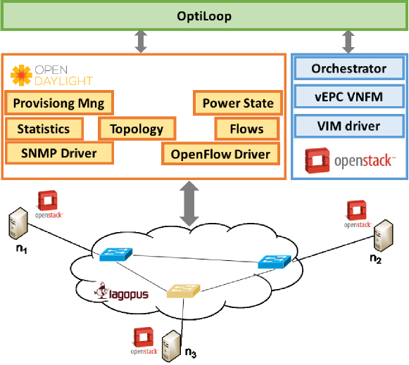
(a)

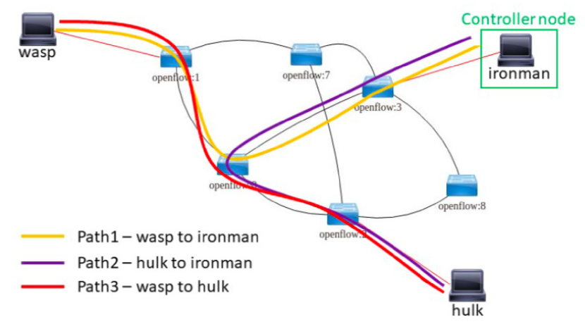
(b)

Figure 5: Architecture (left) and topology (right) of the real-world testbed. Fig. 5(b) also indicates the paths used in our path instantiation experiments, discussed in Sec. VII-A1.

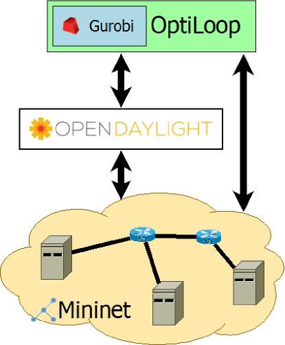
(a)

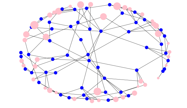
(b)

Figure 6: Architecture (left) and topology (right) of the emulation-based topology. Mininet is used to emulate a network whose topology and traffic match those of a real-world network operator, as discussed in Sec. VI-B1. The size of pink dots is proportional to the traffic generated by the corresponding endpoint.

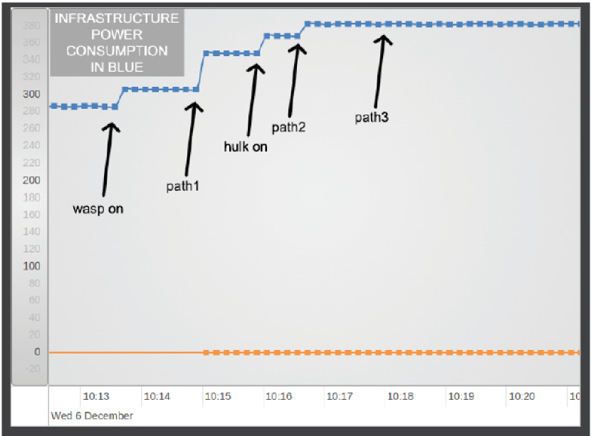
Figure 7: Real-world testbed, path instantiation experiment: evolution of the power consumption of the whole network as the three paths are instantiated. Screenshot from the network orchestrator GUI.

TABLE II: Real-world testbed, path instantiation experiment: power consumption [W]

Condition	Switch $\sharp$1	Switch $\sharp$2	Switch $\sharp$3	Switch $\sharp$4	Switch $\sharp$5	Switch $\sharp$6	All switches
All paths off	21.0299	21.0281	21.02183	20.9614	20.9678	21.0173	125.9841
Path 1 on, no traffic	35.0349	20.9888	35.0096	21.0168	20.9670	34.9968	167.9023
Path 1 on, with traffic	35.4876	21.0455	35.6104	20.9996	21.0180	35.4558	168.2835
Paths 1–2 on, no traffic	35.0309	34.9947	34.9646	20.9988	20.9869	34.9846	181.9242
Paths 1–2 on, with traffic	35.2771	35.2135	35.6386	21.0171	20.9685	35.2783	182.1381
Paths 1–3 on, no traffic	34.9826	34.9894	34.9645	20.9861	20.9693	35.0037	181.9220
Paths 1–3 on, with traffic	35.6249	35.7221	35.5753	21.0042	20.9898	35.5849	183.6007

TABLE III: Real-world testbed, provisioning experiment: delays [s]

Time Component	Maximum	Minimum	Average
OptiLoop	15.117	6.144	9.729
Server activation	0.111	0.068	0.086
Switch activation	2.660	0.871	1.824
Virtual links creation	31.797	21.953	27.369
Single VNF creation	38.823	30.235	31.476
Creation of all VNFs	49.738	31.883	38.384
Network path setup	0.065	0.050	0.056
Single VNF configuration	187.199	53.854	105.860
Configuration of all VNFs	316.992	86.885	216.591
Total NS instantiation	404.868	164.036	299.522

V-D Computational complexity

The fixProblems and saveEnergy procedures are run in order to react to changes in the network load; therefore, it is important that the decisions they make are swift as well as effective. To this end, we can prove that both procedures have polynomial worst-case computational complexity, as stated by the following theorem:

Theorem 1

The fixProblems (Alg. 1) and saveEnergy (Alg. 2) procedures have polynomial worst-case computational complexity.

Proof:

The proof follows by inspection of Alg. 1 and Alg. 2. The algorithms contain no loops, i.e., each of the instructions therein is executed at most once. Among the instruction, all perform elementary operations, except:

• finding the minimum of a set, which requires sorting and has complexity $O(n\log n)$, $n$ being the set size;

• solving convex optimization problems, which has polynomial, namely, cubic computational complexity [19].

Thus, the overall complexity of the fixProblems and saveEnergy procedures is polynomial, namely, cubic. ∎

Theorem 1 ensures that the fixProblems and saveEnergy can be used to make swift and effective decisions in reaction to traffic changes. Indeed, convex optimization problems are routinely [19] solved in embedded applications with real-time requirements.

VI Testbeds, scenario and benchmarks

We validate and evaluate OptiLoop through two testbeds. We study the interaction between OptiLoop, the SDN controller, and the NFVO in a small-scale testbed with real hardware, described in Sec. VI-A. For our performance evaluation we instead use a larger, emulated testbed based on the real-world topology of a mobile operator, as detailed in Sec. VI-B. In all experiments, the reference VNF graph is the vEPC service described in Fig. 1.

VI-A Real-world testbed

The architecture and topology of our real-world testbed are described in Fig. 5. OpenDaylight (Beryllium version) and OpenStack (Mitaka version) are used to control a network made of six Lagopus software switches (with DPDK support enabled for faster switching) and three physical servers, connected as shown in Fig. 5(b). The OpenDaylight SDN controller configures the data plane, by activating/deactivating links and switches via SNMP protocol and configuring the forwarding rules via OpenFlow 1.3 protocol. A custom-built NFVO – integrated with the VNFM (VNF manager) and VIM (Virtual Interface Manager) OpenStack modules – manages the VMs that run the VNFs. Specifically, the NFVO provides RESTful interfaces that allows the orchestration of network services. Services themselves are is composed by multiple VNFs, which are interconnected through the specification of a VNF graph. A detailed description of its architecture and implementation can be found in [20, Sec. 2.6]. We adopt the OpenAirInterface [14] vEPC implementation, including the four VNFs in Fig. 1.

OptiLoop is implemented as a standalone application, written in Java and including two main components, devoted to monitoring and decision-making. OptiLoop interacts with both OpenDaylight and the NFVO through their REST APIs, gathering up-to-date information on the status of switches, links, physical servers and VNFs. When a decision is made, it communicates it to OpenDaylight (if the decision concerns link activation/deactivation) or the NFVO (if the decision concerns VNF deployment or server activation/deactivation). The decision-making component essentially implements Alg. 1 and Alg. 2, using the Gurobi solver for optimization. Since Gurobi features Java bindings, using it within the OptiLoop application is as simple as importing a library.

VI-B Emulated testbed

Our performance evaluation is carried out through an emulated testbed based on Mininet, the de facto standard solution to study SDN-based networks. Its architecture is summarized in Fig. 6(a): similarly to the previous case, OptiLoop interacts with the OpenDaylight controller for network management, and directly with Mininet via its Python API to turn servers and switches on and off. Notice that the actual VNFs are not implemented in Mininet; the traffic they serve is emulated via iperf and the energy consumption is estimated from our real-world testbed, as detailed in Sec. VII-A1 next.

The switches and servers emulated by Mininet reproduce the real-world topology of a major mobile operator, as detailed in Sec. VI-B1. Links and servers are implemented through the TCLink and CPULimitedHost Mininet classes, which allow us to assign them bandwidth, delay and computational capability matching those of their real-world counterparts. All iperf-generated traffic is based on the real-world traffic figures we have access to.

VI-B1 Network topology and traffic

Our reference topology, displayed in Fig. 6(b), represents the real-world topology of a major mobile network operator. It includes 42 endpoints and 51 B/F nodes, with each endpoint connected to exactly two B/F nodes. A total of 1,497 antennas are connected to the endpoints. In the trace, per-endpoint traffic varies between $23.3\text{\,}\mathrm{M}\mathrm{b}\mathrm{i}\mathrm{t}\mathrm{/}\mathrm{s}$ and $148.9\text{\,}\mathrm{M}\mathrm{b}\mathrm{i}\mathrm{t}\mathrm{/}\mathrm{s}$. In order to model future network conditions, we increase such values by accounting for the 22% annual growth rate foreseen by Cisco [21] for the next five years, thus obtaining per-endpoint traffic values varying between $74\text{\,}\mathrm{M}\mathrm{b}\mathrm{i}\mathrm{t}\mathrm{/}\mathrm{s}$ and $473\text{\,}\mathrm{M}\mathrm{b}\mathrm{i}\mathrm{t}\mathrm{/}\mathrm{s}$ per endpoint, with a 82:18 downlink/uplink proportion. The dataset we use only represents a snapshot of the network conditions, i.e., traffic demand does not change over time.

Based on the real-world vEPC implementation [14] we consider a total of four VNFs, namely eNB, MME, HSS, and a gateway implementing both the P-GW and S-GW functions. Notice that in [14] no VNF is split into user- and control-plane sub-entities. We set our $\chi$-values, expressing how traffic gets transformed as it travels between VNFs, leveraging the analysis in [10]; in particular, the fraction of control traffic going to the MME is given by $\chi(\text{eNB},\text{P/S-GW},\text{MME})=0.32$.

Still based on [10], we set the link bandwidth $B_{i,j}$ to $10\text{\,}\mathrm{G}\mathrm{b}\mathrm{i}\mathrm{t}\mathrm{/}\mathrm{s}$ for endpoint-to-node links and $100\text{\,}\mathrm{G}\mathrm{b}\mathrm{i}\mathrm{t}\mathrm{/}\mathrm{s}$ for node-to-node ones. Based on [10] and [22], we assume that each B/F node can process $100\text{\,}\mathrm{G}\mathrm{b}\mathrm{i}\mathrm{t}$ of traffic every second. Since our scenario is constrained by B/F node and link capacity, we ignore network and processing delays.

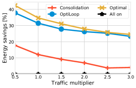
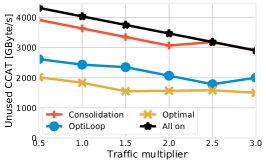
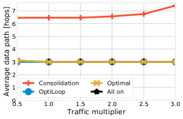
Figure 8: Mininet experiments with real-world topology: energy savings obtained as a function of traffic (left); spare computational capabilities of the active topology (CCAT) (center); number of hops traveled by requests (right).

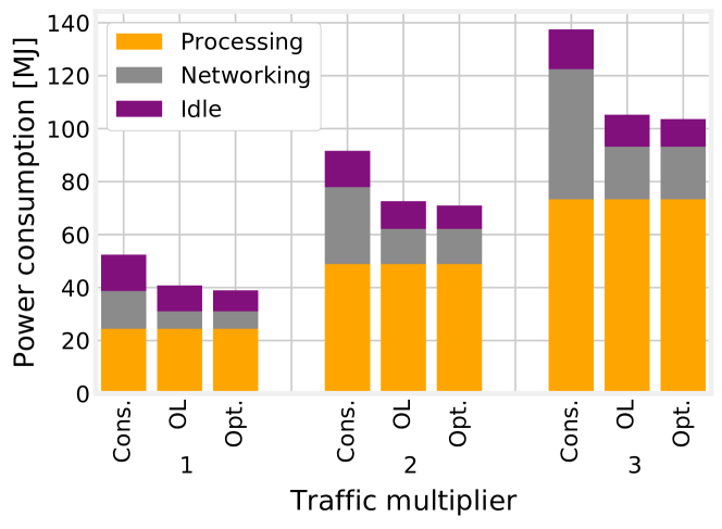
Figure 9: Mininet experiments with real-world topology: breakdown of energy consumption for the consolidation-based (“Cons.”), OptiLoop (“OL”), and optimal (“Opt.”) strategies.

VI-B2 Benchmark solutions

We compare OptiLoop with three alternatives:

• what is done in real-world systems, i.e., keeping all network elements active regardless of traffic, indicated as All on in the plots;

• the optimal solution obtained by brute-force, i.e., trying all possible combinations of network elements to activate, indicated as Optimal in the plots;

• a state-of-the-art approach based on consolidation, based on [7] and indicated as Consolidation in the plots.

The consolidation procedure used in [7] consists of three-stage decision process. For every flow, it first looks for an already-deployed VNF to serve the flow; if none can be found, it deploys a new instance of the VNF at an already active B/F node. If no suitable node is found, it activates a new one. Also, the procedure activates any additional B/F nodes needed to ensure connectivity between endpoints and the serving B/F nodes. It is interesting to notice how all stages of the consolidation design process have the same goals of our fixProblems procedure, namely, ensuring that there is enough computational capability (steps 1 and 2) and network capacity (step 3) to process the incoming traffic. There is no equivalent for the saveEnergy procedure, i.e., already-made decisions are never reconsidered.

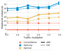
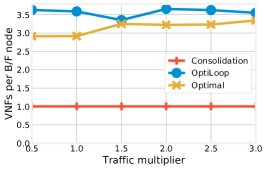
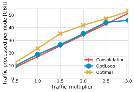
Figure 10: Mininet experiments with real-world topology: number of deployed instances for the eNB and P/S-GW VNFs (left); average number of VNFs deployed in each B/F node (center); average traffic processed at each B/F node (right).

VII Results

We start this section by summarizing, in Sec. VII-A, the power consumption and delay figures we obtain from the real-world testbed described in Sec. VI-A. We then present, in Sec. VII-B, a performance evaluation of OptiLoop carried out by emulating a real-world topology in Mininet, as described in Sec. VI-B.

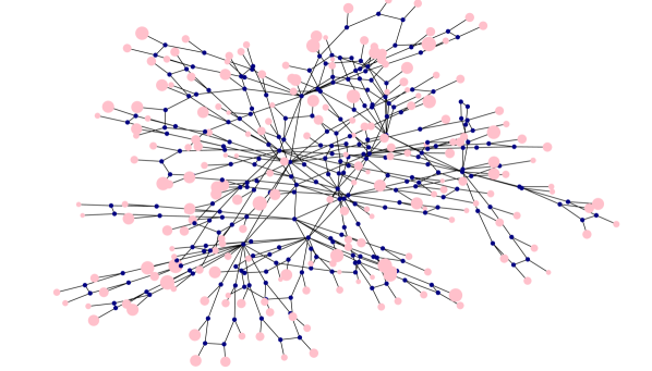
Figure 11: Scaled-up network topology. As in Fig. 6, blue dots indicate B/F nodes, pink ones indicate endpoints, and the size of pink dots is proportional to the traffic generated by the corresponding endpoint.

VII-A Results from the real-world testbed

There are two main types of information we seek to obtain from the real-world testbed described in Sec. VI-A:

• the power consumption associated with B/F nodes, broken down in idle and processing power;

• the delay associated with changes to the network, e.g., activating a link or instantiating a new VM.

We measure the above quantities through two experiments, namely, a path instantiation experiment and a service provisioning one, as described next.

VII-A1 Path instantiation experiment

In this experiment, we start with all equipment – switches and servers – in sleeping mode. We then instantiate, one by one, the three paths shown in Fig. 5(b), activating additional switches as needed. Finally, we generate bidirectional flows of $1\text{\,}\mathrm{G}\mathrm{b}\mathrm{y}\mathrm{t}\mathrm{e}\mathrm{/}\mathrm{s}$ between each pair of endpoints, so as to ascertain the impact of traffic on the power consumption.

The evolution of the power consumption in our real-world testbed is exemplified in Fig. 7. In the beginning, when all network elements are in sleeping mode, the total power consumption is around $280\text{\,}\mathrm{W}$. Activating new servers results in an increase in power consumption, as can be expected. More interestingly, instantiating a new path results in a power increase only if it requires activating a new switch, as is the case of path 1 and path 2. As we can see from Fig. 5(b), path 3 requires no extra switches with respect to path 1 and path 2, and therefore instantiating it results in no additional consumption.

Tab. II provides a more analytical view of the power consumed by the switches in different states. When all equipment is in sleeping mode (first row), each switch consumes roughly $21\text{\,}\mathrm{W}$ of power. Instantiating path 1 (second row) requires activating switches 1–3 and 6, whose power consumption jumps to $35\text{\,}\mathrm{W}$; activating additional paths has the same effect on the other switches. We can also observe that sending traffic over the instantiated paths has a noticeable, but minor, effect: routing $1\text{\,}\mathrm{G}\mathrm{b}\mathrm{y}\mathrm{t}\mathrm{e}\mathrm{/}\mathrm{s}$ of traffic results in an additional consumption of around $0.5\text{\,}\mathrm{W}$ per switch. Finally, notice that the last column of Tab. II does not match the line in Fig. 7 since the latter also includes the consumption of the physical servers, i.e., $80\text{\,}\mathrm{W}$ in sleeping mode and roughly $120\text{\,}\mathrm{W}$ when active.

VII-A2 Service provisioning experiment

In the service provision experiment, we are interested in measuring the delay associated with performing changes to the network, including path instantiation and service provisioning. To this end, we use the network described in Sec. VI-A to provide the virtual EPC (vEPC) service, consisting of the VNFs depicted in Fig. 1, as implemented in [14].

Doing so requires three main steps, namely (i) making VNF placement and traffic routing decisions, i.e., running OptiLoop; (ii) setting up the required paths, similar to the path instantiation experiment described in Sec. VII-A1; (iii) instantiating and configuring the VMs that run the VNFs. The aspect we are chiefly interested in is the relative importance of such delay components. The results are summarized in Tab. III. A first, important observation is that OptiLoop only accounts for a small fraction (roughly 3%) of the total delay; in other words, the energy savings it brings come at a modest price in terms of additional delay.

Among the other delay components, we can observe that VM configuration and, to a lesser extent, virtual link creation dominate the total delay. It is also interesting to notice the values labeled “Creation of all VNFs” and “Configuration of all VNFs”, which are substantially less than four times the creation (resp. configuration) of a single VNF. This is because, once decisions are made by OptiLoop, they can be implemented in a parallel fashion.

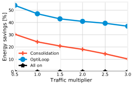
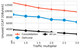
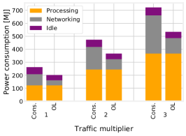
Figure 12: Mininet experiments with scaled-up topology: savings obtained as a function of traffic (left); spare computational capabilities of the active topology (CCAT) (center); energy consumption breakdown (right). Traffic multipliers are referred to the scaled-up traffic, i.e., five times the traffic in the original trace described in Sec. VI-B1.

VII-B Emulation-based performance evaluation

The first answer we seek from the performance evaluation carried out through the emulated testbed concerns the magnitude of possible energy savings. In Fig. 8(left), we vary the traffic demand between 0.5 and 3 times the real-world amount, and study how much energy we can save compared to what is done today, i.e., leaving all B/F nodes and links active. We can observe that OptiLoop yields dramatic savings, consistently very close to the optimum, while consolidation does not perform as well. An intuitive reason is that OptiLoop accounts for all the three main contributions to energy consumption (processing, idle power, and networking), while the consolidation-based approach focuses on keeping the number of active B/F nodes low.

Fig. 8(center) shows the spare computational capability of the active topology (CCAT); intuitively, this is a measure of how much power is being wasted, i.e., how inefficient the network management strategy is. The consolidation algorithm has the highest spare CCAT, because of the higher number of B/F nodes that have to be activated in order to guarantee connectivity. The spare CCAT yielded by OptiLoop is much lower, and very close to the optimum. It is interesting to remark that even the optimum leaves substantial spare CCAT. This is due to the fact that some B/F nodes have to be active in order to keep the topology connected, even if they do not have to host any VNF. Fig. 8(right) depicts how many hops data travels across the network. OptiLoop again matches the optimum, while the consolidation strategy results in substantially longer paths, due to the fact that VNF placement decisions are made without accounting for connectivity.

We now use the power consumption we measure from our real-world testbed (Sec. VII-A) to extrapolate the total power that the emulated network would consume. Fig. 9 breaks such a consumption into its main components, namely, processing, networking, and idle power. Note that these components have comparable magnitude, i.e., none of them dominates the overall consumption. It follows that network management strategies have to account for them all. We can also see that the processing component never changes across strategies, since the amount of traffic to process is always the same. The difference between the strategies lies mostly in the networking component (longer paths in Fig. 8(right) correspond to higher consumption) and, to a lesser extent, in the idle energy. In other words, it is important to place VNFs close to the traffic they have to serve, while at the same time activating as few B/F nodes as possible.

Dropping the “all on” strategy to keep plots easy to read, Fig. 10(left) and Fig. 10(center) show that placing VNFs close to the traffic they serve also means placing many of them. This goes against the traditional concept of activating only the strictly required number of elements, and it is a direct consequence of the features of modern, software-based networks. Indeed, there is little or no penalty for placing an underutilized VNF instance on an already active B/F node, while there is a significant energy cost for transferring even modest amounts of data between B/F nodes. Indeed, we can say that OptiLoop outperforms state-of-the-art alternatives because it properly accounts for the unique features of 5G, thus being more aggressive in deploying VNFs.

Comparing Fig. 10(left) to Fig. 10(center), we can see that OptiLoop deploys more VNFs than the optimum, but the number of VNFs per B/F node is similar. This is because OptiLoop activates slightly more B/F nodes than the optimum, as confirmed by Fig. 10(right) showing that the average amount of traffic processed per B/F node is slightly lower in OptiLoop.

VII-C Scaled-up network topology

In the following, we investigate the performance of OptiLoop when used on larger-scale network topologies. To this end, based on indications from the mobile operator that provided us with the original topology described in Sec. VI-B1, we generate a scaled-up version thereof. Specifically, we operate as follows:

1. we replace each B/F node of the original topology with a ring of five B/S nodes;

2. we place an additional 160 endpoints connected to 6,000 additional antennas;

3. we connect each additional endpoint to two randomly-chosen B/S nodes;

4. we set the traffic requested by the additional antennas in such a way that the traffic distribution matches the original one, scaled up by a factor of five.

The resulting topology, depicted in Fig. 11, has over 200 B/F nodes serving traffic coming from 7,500 antennas. The results yielded by OptiLoop and the consolidation algorithm are reported in Fig. 12. Notice that there are no “optimal” curves, as computing the optimum for the scaled-up topology proved utterly impractical.

Fig. 12(left) shows that, as the topology gets larger, OptiLoop – and, to a lesser extent, consolidation – yield more savings, almost reaching 50%. Intuitively, this is connected to the fact that in larger topologies it is easier to maintain connectivity while deactivating a substantial fraction of B/F nodes. This is confirmed by Fig. 12(center), showing that the spare CCAT, i.e., the unused computational power in the active network, is proportionally lower than in the original topology. Indeed, as we can see from Fig. 8(center), the spare CCAT with the original topology reaches 2,500 units under OptiLoop, while in Fig. 12(center) it is below 10,000 units in spite of the topology being five times larger.

Finally, Fig. 12(right) breaks the total power consumption into its main components. By comparing it with Fig. 9, we can observe that:

• the processing power is exactly five times larger than in the original topology, as that component is strictly proportional to the traffic to serve;

• the idle power is proportionally lower since, as observed earlier, there are fewer B/F nodes activated only for sake of connectivity;

• the networking power is proportionally larger, as data are more likely to travel a longer path to the serving B/F node.

The latter two items suggest that networking power and idle power are, to a certain extent, antithetical, and it can be hard to minimize both at the same time.

VIII Conclusion

We considered two of the unique features of 5G networks, namely, the hybrid nature of their nodes (which have both forwarding and computational capabilities) and the fact that the traffic to serve changes across processing steps. Such features require the entities in the MANO layer, and especially the NFVO, to make joint decisions about (i) which B/F nodes to activate, (ii) the VNF instances they run, and (iii) how to route traffic between VNFs and the nodes running them. We formulated a system model and optimization problem, that enable us to make all such decisions with the objective to minimize the energy consumption of the network. We further proposed OptiLoop, a solution concept based on integrating optimization within the MANO entities, allowing them to make decisions by repeatedly solving relaxed optimization problems.

We validated OptiLoop through a real-world testbed based on OpenDaylight and OpenStack, and further evaluated its performance through a large-scale emulated network whose topology and traffic are based on those of a major network operator. OptiLoop was shown to outperform state-of-the-art approaches and closely track the optimum, while representing only a minor contribution to the total network delay.

References

- [1] N. Gazit, F. Malandrino, and D. Hay, “Coopetition between network operators and content providers in SDN/NFV core networks,” in IEEE INFOCOM SWFAN Workshop, 2016.
- [2] R. Cohen, L. Lewin-Eytan, J. S. Naor, and D. Raz, “Near optimal placement of virtual network functions,” in IEEE INFOCOM, 2015.
- [3] L. Wang, Z. Lu, X. Wen, R. Knopp, and R. Gupta, “Joint Optimization of Service Function Chaining and Resource Allocation in Network Function Virtualization,” IEEE Access, 2016.
- [4] T.-W. Kuo, B.-H. Liou, K. C.-J. Lin, and M.-J. Tsai, “Deploying chains of virtual network functions: On the relation between link and server usage,” in IEEE INFOCOM, 2016.
- [5] L. Qu, C. Assi, and K. Shaban, “Delay-aware scheduling and resource optimization with network function virtualization,” IEEE Trans. on Communications, 2016.
- [6] X. Zhang, Z. Huang, C. Wu, Z. Li, and F. C. Lau, “An Online Stochastic Buy-Sell Mechanism for VNF chains in the NFV market,” IEEE Journal on Selected Areas in Communications, 2017.
- [7] N. El Khoury, S. Ayoubi, and C. Assi, “Energy-Aware Placement and Scheduling of Network Traffic Flows with Deadlines on Virtual Network Functions,” in IEEE CloudNet, 2016.
- [8] V. G. Nguyen, A. Brunstrom, K. J. Grinnemo, and J. Taheri, “SDN/NFV-based Mobile Packet Core Network Architectures: A Survey,” IEEE Communications Surveys Tutorials, 2017.
- [9] A. Baumgartner, V. S. Reddy, and T. Bauschert, “Mobile core network virtualization: A model for combined virtual core network function placement and topology optimization,” in IEEE NetSoft, 2015.
- [10] G. Hasegawa and M. Murata, “Joint Bearer Aggregation and Control-Data Plane Separation in LTE EPC for Increasing M2M Communication Capacity,” in IEEE GLOBECOM, 2015.
- [11] S. Khairi, M. Bellafkih, and B. Raouyane, “QoS management SDN-based for LTE/EPC with QoE evaluation: IMS use case,” in SDS, 2017.
- [12] X. An, W. Kiess, J. Varga, J. Prade, H.-J. Morper, and K. Hoffmann, “SDN-based vs. software-only EPC gateways: A cost analysis,” in IEEE NetSoft, 2016.
- [13] J. Prados-Garzon, J. J. Ramos-Munoz, P. Ameigeiras, P. Andres-Maldonado, and J. M. Lopez-Soler, “Modeling and Dimensioning of a Virtualized MME for 5G Mobile Networks,” IEEE Trans. on Veh. Tech., 2017.
- [14] OpenAirInterface: 5G software alliance for democratising wireless innovation. http://www.openairinterface.org.
- [15] D. Dietrich, C. Papagianni, P. Papadimitriou, and J. S. Baras, “Network function placement on virtualized cellular cores,” in COMSNETS, 2017.
- [16] F. Malandrino, C. F. Chiasserini, C. E. Casetti, and G. Landi, “Optimization-in-the-Loop for Energy-Efficient 5G,” in IEEE WoWMoM, 2018.
- [17] ETSI. (2017) Network Functions Virtualisation (NFV); Management and Orchestration. http://www.etsi.org/deliver/etsi_gs/NFV-MAN/001_099/001/01.01.01_60/gs_NFV-MAN001v010101p.pdf.
- [18] J. Mattingley and S. Boyd, “Cvxgen: A code generator for embedded convex optimization,” Optimization and Engineering, 2012.
- [19] S. Boyd and L. Vandenberghe, Convex optimization. Cambridge university press, 2004.
- [20] 5G Crosshaul Project. Deliverable D3.2: Final XFE/XCI design and specification of southbound and northbound interfaces. http://5g-crosshaul.eu/wp-content/uploads/2018/01/5G-CROSSHAUL_D3.2.pdf.
- [21] Cisco, “Cisco Visual Networking Index,” 2017.
- [22] Lagopus Project. It’s kind of fun to do the impossible with DPDK. https://www.slideshare.net/lagopus/dpdk-summit-2015-its-kind-of-fun-to-do-the-impossible-with-dpdk.