HD 965: An extremely peculiar A star
with an extremely long rotation period

Abstract

Context. One of the keys to understanding the origin of the Ap stars and their significance in the general context of stellar astrophysics is the consideration of the most extreme properties displayed by some of them. In that context, HD 965 is particularly interesting, as it combines some of the most pronounced chemical peculiarities with one of the longest rotation periods known.

Aims. We characterise the variations of the magnetic field of the Ap star HD 965 and derive constraints about its structure.

Methods. We combine published measurements of the mean longitudinal field $\langle B_{z}\rangle$ of HD 965 with new determinations of this field moment from circular spectropolarimetry obtained at the 6-m telescope BTA of the Special Astrophysical Observatory of the Russian Academy of Sciences. For the mean magnetic field modulus $\langle B\rangle$, literature data are complemented by the analysis of ESO archive spectra.

Results. We present the first determination of the rotation period of HD 965, $P_{\rm rot}=(16.5\pm 0.5)$ y. HD 965 is only the third Ap star with a period longer than 10 years for which magnetic field measurements have been obtained over more than a full cycle. The variation curve of $\langle B_{z}\rangle$ is well approximated by a cosine wave. $\langle B\rangle$ does not show any significant variation. The observed behaviour of these field moments is well represented by a simple model consisting of the superposition of collinear dipole, quadrupole and octupole. The distribution of neodymium over the surface of HD 965 is highly non-uniform. The element appears concentrated around the magnetic poles, especially the negative one.

Conclusions. The shape of the longitudinal magnetic variation curve of HD 965 indicates that its magnetic field is essentially symmetric about an axis passing through the centre of the star. Overall, as far as its magnetic field is concerned, HD 965 appears similar to the bulk of the long-period Ap stars.

1 Introduction

Svolopoulos (1963) appears to have been the first to notice the peculiarity of the spectrum of HD 965 (= BD $-$0 21), a star of spectral type A8p SrEuCr according to Renson & Manfroid (2009). Very little attention was paid to this star until it was found to have resolved magnetically split lines (Mathys et al. 1997). The subsequent effort that was undertaken to study its magnetic field suggested the possible occurrence of the core-wing anomaly (CWA) in the hydrogen Balmer lines, a suspicion that was soon confirmed by means of a dedicated observation (Cowley et al. 2001). This indicates that the structure of the atmosphere of HD 965 cannot be represented by a normal A-star model atmosphere. It has also been reported that the magnetic field of HD 965 decreases with increasing optical depth (Nesvacil et al. 2004), but more observations would be needed for full characterisation of its structure. More generally, the spectrum of HD 965 is extremely peculiar, bearing considerable resemblance to that of Przybylzki’s star (HD 101065), the Ap star with the most unusual spectrum (Hubrig et al. 2002). Like Przybylski’s star, HD 965 shows in its spectrum spectral lines that have been tentatively attributed to promethium, an unstable element (Cowley et al. 2004).

The presence of the CWA in its spectrum motivated a photometric search for rapid oscillations in HD 965. Despite the high precision of the observations, no such oscillations were detected (Kurtz et al. 2003). A subequent attempt using high-cadence high-resolution spectroscopy did not yield any detection either (Elkin et al. 2005).

Besides its extreme and intriguing spectral features, HD 965 also has the distinction of rotating exceptionally slowly. Mathys (2017) reported that its rotation period must exceed 13 y. This puts it firmly among the group of Ap stars with rotation periods longer than one month. This group, which has been progressively emerging in recent years, comprises several percent of the whole Ap star class. Studying it is essential for the understanding of the processes responsible for the differentiation of stellar rotation rates. This has been discussed in more detail elsewhere (Mathys et al. 2019).

In this paper, we present new determinations of the mean longitudinal magnetic field $\langle B_{z}\rangle$ and of the mean magnetic field modulus $\langle B\rangle$ of HD 965. They are based on both new dedicated observations and archive spectra. We use the complete set of existing $\langle B_{z}\rangle$ measurements of the star to determine for the first time the value of its rotation period. The observational data and their analysis are presented in Sect. 2, and the determination of the stellar rotation period is described in Sect. 3. In Sect. 4, we derive constraints on the geometrical structure of the magnetic field. Finally, we discuss the implications of the obtained results for HD 965 itself, and how it fits within the general context of the slowly rotating Ap stars.

2 Observations and data analysis

2.1 Mean magnetic field modulus

The mean magnetic field modulus $\langle B\rangle$ is the average over the visible stellar hemisphere of the modulus of the field vector, weighted by the local emergent line intensity.

All the mean field modulus values used in this analysis were determined from the measured wavelength separation of the two magnetically split components of the Fe ii $\lambda\,6149.2$ diagnostic line. The following formula was applied to derive $\langle B\rangle$:

$$\lambda_{\rm r}-\lambda_{\rm b}=g\,\Delta\lambda_{\rm Z}\,\langle B\rangle\,.$$ (1)

In this equation, $\lambda_{\rm r}$ and $\lambda_{\rm b}$ are, respectively, the wavelengths of the red and blue split line components; $g$ is the Landé factor of the split level of the transition ($g=2.70$; Sugar & Corliss 1985); $\Delta\lambda_{\rm Z}=k\,\lambda_{0}^{2}$, with $k=4.67\,10^{-13}$ Å^-1 G^-1; $\lambda_{0}=6149.258$ Å is the nominal wavelength of the considered transition.

The application of the above-described procedure is complicated by the fact that the Fe ii $\lambda\,6149.2$ line is strongly blended on the blue side with an unidentified rare earth line. This blend is present at different degrees in a fraction of the Ap stars. As can be seen e.g. in Figs. 2 to 4 of Mathys et al. (1997), HD 965 is one of the stars in which its impact is most severe. Dealing with this blend as consistently as possible in measuring the separation of the split components of the Fe ii $\lambda\,6149.2$ line in spectra of HD 965 obtained at different epochs is essential to achieve the best precision and uniformity in the derived values of $\langle B\rangle$. This precision and uniformity are required to ensure that the variations of $\langle B\rangle$ along the stellar rotation cycle can be correctly characterised.

Table 1: Mean magnetic field modulus measurements.

JD	$\langle B\rangle$ (G)	Configuration
2449301.597	4320	ESO CAT + CES SC
2449534.896	4366	ESO CAT + CES LC
2449535.879	4306	ESO CAT + CES LC
2449881.918	4247	ESO CAT + CES LC
2449908.843	4263	ESO CAT + CES LC
2449947.836	4268	ESO CAT + CES LC (lower res.)
2450231.914	4199	ESO CAT + CES LC
2450296.576	4386	OHP 1.52 m + AURELIE
2450971.914	4256	ESO CAT + CES LC
2451042.807	4326	ESO CAT + CES LC
2451084.731	4192	ESO CAT + CES LC
2451740.105	4234	CFHT + Gecko
2451741.060	4264	CFHT + Gecko
2452190.627	4303	ESO VLT UT2 + UVES
2452420.063	4228	CFHT + Gecko
2452535.723	4352	ESO VLT UT2 + UVES
2452924.154	4293	ESO VLT UT2 + UVES
2453215.093	4287	CFHT + Gecko
2453334.505	4213	ESO 3.6 m + HARPS
2453581.741	4165	ESO 3.6 m + HARPS
2453582.764	4225	ESO 3.6 m + HARPS
2453583.867	4242	ESO 3.6 m + HARPS
2453661.702	4279	ESO VLT UT2 + UVES
2453711.565	4237	ESO 3.6 m + HARPS
2453712.595	4177	ESO 3.6 m + HARPS
2453713.585	4201	ESO 3.6 m + HARPS
2453714.583	4238	ESO 3.6 m + HARPS
2453715.568	4208	ESO 3.6 m + HARPS
2453716.567	4245	ESO 3.6 m + HARPS
2454336.860	4185	ESO 3.6 m + HARPS
2454338.796	4215	ESO 3.6 m + HARPS
2454406.585	4310	ESO VLT UT2 + UVES
2454442.613	4224	ESO 3.6 m + HARPS
2454443.560	4186	ESO 3.6 m + HARPS
2454469.580	4259	ESO VLT UT2 + UVES

Table 2: Mean longitudinal magnetic field measurements.

JD S/N $\langle B_{z}\rangle$ $\sigma_{z}$ Reference (G) (G) 2449916.907 140 $-$574 113 Mathys (2017) 2449974.744 110 $-$691 141 Mathys (2017) 2450039.588 120 $-$863 44 Mathys (2017) 2450294.905 120 $-$1063 125 Mathys (2017) 2450615.928 120 $-$1057 52 Mathys (2017) 2450629.884 125 $-$1159 142 Mathys (2017) 2450784.596 150 $-$1270 139 Mathys (2017) 2451806.479 100 $-$430 120 Elkin et al. (2005) 2452130.497 100 $-$360 70 Elkin et al. (2005) 2452153.356 40 $-$280 120 Elkin et al. (2005) 2452625.209 90 $-$160 80 Elkin et al. (2005) 2452626.232 90 $-$80 50 Elkin et al. (2005) 2452831.529 180 $-$30 80 Elkin et al. (2005) 2453273.296 190 320 50 Elkin et al. (2005) 2453362.231 300 360 30 Romanyuk et al. (2015) 2453666.290 330 330 40 Romanyuk et al. (2015) 2453667.270 250 470 40 Romanyuk et al. (2015) 2453718.245 450 420 30 Romanyuk et al. (2015) 2453953.425 350 600 40 Romanyuk et al. (2015) 2454015.236 350 420 50 Romanyuk et al. (2015) 2454402.285 300 530 50 Romanyuk et al. (2014) 2455017.511 250 150 40 Romanyuk et al. (2016) 2455075.438 300 240 50 Romanyuk et al. (2016) 2455431.458 250 $-$70 20 Romanyuk et al. (2017) 2455459.492 250 $-$240 50 Romanyuk et al. (2017) 2455461.462 300 $-$140 50 Romanyuk et al. (2017) 2455553.174 300 $-$340 20 Romanyuk et al. (2017) 2455555.139 200 $-$360 30 Romanyuk et al. (2017) 2455583.148 180 $-$359 26 Romanyuk et al. (2018) 2455842.411 250 $-$624 23 Romanyuk et al. (2018) 2455843.398 250 $-$643 23 Romanyuk et al. (2018) 2455871.176 150 $-$470 29 Romanyuk et al. (2018) 2455962.138 150 $-$590 30 Romanyuk et al. (2015)

JD S/N $\langle B_{z}\rangle$ $\sigma_{z}$ Reference (G) (G) 2456174.540 200 $-$670 40 Romanyuk et al. (2015) 2456177.429 300 $-$800 50 Romanyuk et al. (2015) 2456234.208 110 $-$1030 30 Romanyuk et al. (2015) 2456500.509 160 $-$1190 20 Romanyuk et al. (2015) 2456589.383 160 $-$1250 20 Romanyuk et al. (2015) 2456640.125 150 $-$1130 50 Romanyuk et al. (2015) 2456940.302 150 $-$1170 30 Romanyuk et al. (2015) 2456967.292 150 $-$1130 60 Romanyuk et al. (2015) 2456995.144 200 $-$1360 50 Romanyuk et al. (2015) 2457169.525 150 $-$1340 30 Romanyuk et al. (2015) 2457246.465 200 $-$1200 20 Romanyuk et al. (2015) 2457288.469 200 $-$1170 20 This paper 2457352.232 150 $-$1110 40 This paper 2457355.195 200 $-$1120 20 This paper 2457592.479 120 $-$1090 40 This paper 2457740.260 100 $-$910 60 This paper 2457761.132 130 $-$960 30 This paper 2457762.156 120 $-$920 30 This paper 2457764.149 120 $-$1070 50 This paper 2457950.436 180 $-$990 30 This paper 2458006.458 110 $-$780 20 This paper 2458009.364 100 $-$820 30 This paper 2458061.227 130 $-$680 30 This paper 2458067.216 150 $-$780 30 This paper 2458116.161 140 $-$610 30 This paper 2458117.213 150 $-$690 30 This paper 2458126.137 150 $-$650 20 This paper 2458151.136 120 $-$740 20 This paper 2458447.277 150 $-$320 20 This paper 2458448.298 170 $-$340 30 This paper 2458449.162 100 $-$290 40 This paper 2458512.155 160 $-$260 40 This paper

Obviously, we cannot be sure that the way in which we measure HARPS and UVES archive spectra at present is consistent with the way in which spectra obtained (mostly) with other instruments were measured in the past to derive the published values of $\langle B\rangle$ (Mathys et al. 1997; Elkin et al. 2005; Mathys 2017). Accordingly, to ensure that the set of mean magnetic field modulus data under consideration is as uniform as possible, we remeasured all the spectra of the cited references and used them to derive updated $\langle B\rangle$ values. Thus, the full set of observations that we analysed consists of:

• 9 spectra recorded with the Long Camera (LC) of the Coudé Echelle Spectrograph (CES) fed by the ESO Coudé Auxiliary Telescope (CAT), one of which had a somewhat lower resolution than the others owing to a detector problem;

• 1 spectrum recorded with the Short Camera (SC) of the CES, fed by the CAT;

• 1 spectrum recorded with the AURELIE spectrograph fed by the 1.52-m telescope of the Observatoire de Haute-Provence (OHP);

• 4 spectra recorded with the Gecko spectrograph fed by the Canada-France-Hawaii Telescope (CFHT);

• 6 spectra recorded with the Ultraviolet and Visible Echelle Spectrograph (UVES) fed by Unit Telescope 2 (UT2) of the ESO Very Large Telescope (VLT). One of them is the average of the 111 high-cadence spectra analysed by Elkin et al. (2005); the others were retrieved from the ESO Archive;

• 14 spectra recorded with the High Accuracy Radial velocity Planet Searcher (HARPS) fed by the ESO 3.6-m telescope, retrieved from the ESO Archive.

More details about the first four configurations of this list and the corresponding data reduction processes are provided by Mathys et al. (1997). See also Elkin et al. (2005) for information about the reduction of the respective observations. For the other UVES observations, and for the HARPS spectra, we used science grade pipeline processed data available from the ESO Archive. The only additional processing that we carried out was a continuum normalisation of the region ($\sim$100 Å wide) surrounding the Fe ii $\lambda\,6149.2$ diagnostic line.

The challenge that we met to achieve consistent measurements of the wavelength separation of the split components of the Fe ii $\lambda\,6149.2$ line despite the heavy blending of its blue wing led us to revise the estimate of the uncertainty affecting the derived $\langle B\rangle$ values that had been adopted by Mathys et al. (1997) and by Mathys (2017). The latter, 30 G, is definitely too optimistic, as it is of the same order as the estimated $\langle B\rangle$ uncertainty for stars such as HD 50169, for which measuring the wavelength splitting of the Fe ii $\lambda\,6149.2$ line is definitely much more straightforward (Mathys et al. 2019). Taking this into account, and after comparing the results of measurements of a number of spectra repeated multiple times, we now adopt 50 G as a revised estimate, hopefully more realistic, of the uncertainty affecting the determinations of the mean magnetic field modulus of HD 965.

The 35 values of the mean magnetic field modulus obtained in the above-described way are presented in Table 1. The columns give, in order, the Heliocentric (or Barycentric, for HARPS) Julian Date of mid-exposure, the value $\langle B\rangle$ of the mean magnetic field modulus, and the instrumental configuration with which the analysed spectrum was obtained.

2.2 Mean longitudinal magnetic field

The mean longitudinal magnetic field $\langle B_{z}\rangle$ is the average over the visible hemisphere of the component of the magnetic vector along the line of sight, weighted by the local emergent line intensity. The following published measurements of this field moment were used in this study:

• 7 measurements from Elkin et al. (2005);

• 1 measurement from Romanyuk et al. (2014);

• 18 measurements from Romanyuk et al. (2015);

• 2 measurements from Romanyuk et al. (2016);

• 7 measurements from Mathys (2017);

• 5 measurements from Romanyuk et al. (2017);

• and 4 measurements from Romanyuk et al. (2018).

All these measurements were carried out through the analysis of medium spectral resolution observations of metal lines in circular polarisation. The data from Mathys (2017) are based on observations obtained with the CASPEC spectrograph mounted on the ESO 3.6 m telescope, in the post-1995 configuration specified by Mathys & Hubrig (1997). All other listed studies were carried out with the instrumentation introduced in the next paragraph.

Here the measurements from the literature are complemented by additional $\langle B_{z}\rangle$ determinations obtained from observations of the same type, that is, spectra of HD 965 recorded at $R\simeq 14\,500$ in both circular polarisations with the Main Stellar Spectrograph of the 6-m telescope BTA of the Special Astrophysical Observatory (SAO), on 21 nights spread from September 2015 to January 2019. This is the same configuration as used by Romanyuk et al. (2014), and in the other works of the same group. The instrumental configuration and the data reduction procedure are as described in detail in this reference.

The mean longitudinal magnetic field was determined from the wavelength shifts of a sample of spectral lines between the two circular polarisations in each of these spectra, by application of the formula:

$$\lambda_{\rm R}-\lambda_{\rm L}=2\,\bar{g}\,\Delta\lambda_{\rm Z}\,\langle B_{z}\rangle\,,$$ (2)

where $\lambda_{\rm R}$ (resp. $\lambda_{\rm L}$) is the wavelength of the centre of gravity of the line in right (resp. left) circular polarisation and $\bar{g}$ is the effective Landé factor of the transition. $\langle B_{z}\rangle$ is determined through a least-squares fit of the measured values of $\lambda_{\rm R}-\lambda_{\rm L}$ by a function of the form given above. The standard error $\sigma_{z}$ that is derived from that least-squares analysis is used as an estimate of the uncertainty affecting the obtained value of $\langle B_{z}\rangle$. The implementation details have been described by Mathys (2017) for the analysis of the CASPEC observations, and by Romanyuk et al. (2014) and by Romanyuk et al. (2015) for the SAO spectra. Whenever both the modernised Babcock method and the regression method were applied for determination of $\langle B_{z}\rangle$ from these spectra, the value yielded by the regression method was adopted. For HD 965, the differences between the mean longitudinal values derived through application of either method (Romanyuk et al. 2015) are insignificant.

The values of the mean longitudinal field obtained in the way described above are presented in Table 2. For the convenience of the reader, this table also includes the previously published measurements. In total, 65 $\langle B_{z}\rangle$ measurements are analysed in this study. The table columns give, in order, the Heliocentric Julian Date of mid-observation, the mean S/N ratio of the recorded spectrum, the value $\langle B_{z}\rangle$ of the mean longitudinal magnetic field and its uncertainty $\sigma_{z}$, and the source of the measurement.

3 Variability and rotation period

To determine the rotation period of HD 965, we fitted the measurements of its mean longitudinal magnetic field by either a cosine wave, or the superposition of a cosine wave and of its first harmonic, progressively varying the period of these waves, in search of the value of the period that minimises the reduced $\chi^{2}$ of the fit. These fits are weighted by the inverse of the square of the uncertainties of the individual measurements. Through this procedure, we concluded unambiguously that the rotation period of the star must be of the order of 6000 d. The corresponding periodogram is shown in Fig. 3.

The time elapsed between the first determination of the mean longitudinal magnetic field of HD 965 by Mathys (2017) and our most recent spectropolarimetric observation of the star is 8596 d, or $\sim$1.4 rotation period. This provides a very sensitive approach to refine the determination of the period and to estimate its uncertainty. By plotting a phase diagram of the $\langle B_{z}\rangle$ measurements for a series of tentative values of the period around the one suggested by the periodogram, one can visually identify the period value that minimises the phase shifts between field determinations from different rotation cycles, and constrain the range around that value for which those phase shifts remain reasonably small.

Determinations of $\langle B_{z}\rangle$ obtained with different instruments and by application of different data analysis methods are known to show frequently systematic differences, whose existence between the two sets of data of interest cannot be definitely ruled out. However, previous studies indicate that, in general, for Ap stars with fairly sharp spectral lines, there are at most minor systematic differences between the longitudinal field values determined, through application of the metal line spectropolarimetric technique, by Mathys and collaborators (from ESO CASPEC spectra), and by Romanyuk and collaborators (with the Main Stellar Spectrograph of the 6-m telescope BTA of the SAO). One can also note that, as the spectral range spanned by the SAO spectra has increased over time (Romanyuk et al. 2015), different sets of lines have been measured at different epochs, without introducing any obvious inconsistency in the derived $\langle B_{z}\rangle$ values.

Assuming that the $\langle B_{z}\rangle$ datasets that we combine here are indeed mutually consistent, we derived the following best value of the rotation period of HD 965:

$$P_{\rm rot}=(6030\pm 200)\,\mathrm{d}.$$ (3)

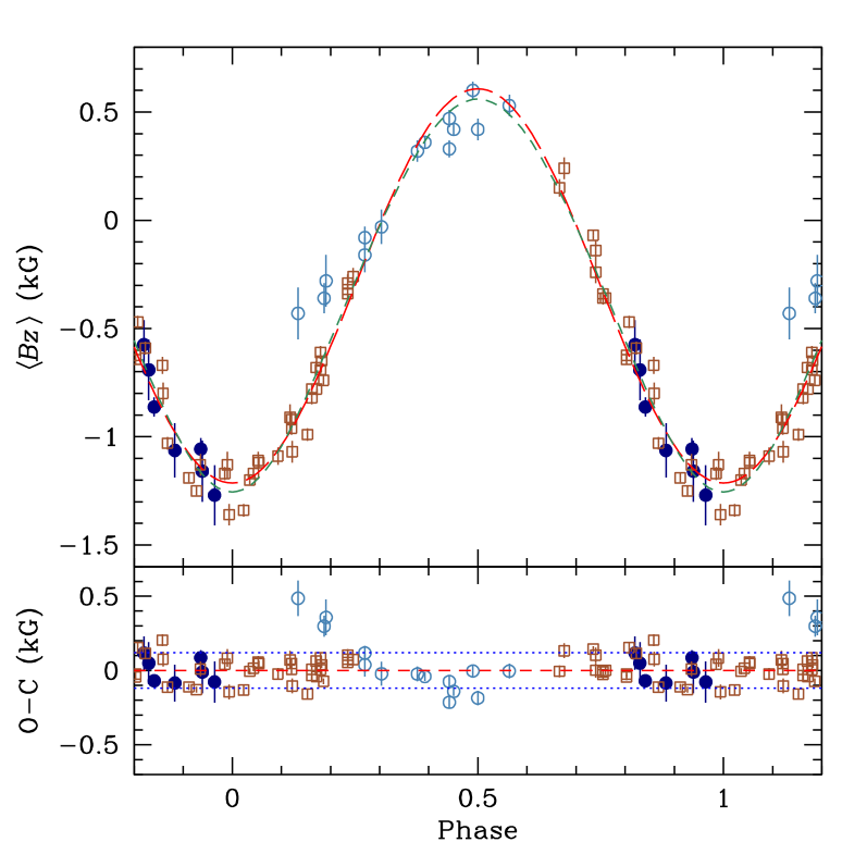
Figure 1: Upper panel: Mean longitudinal magnetic field of HD 965 against rotation phase. To distinguish measurements obtained at similar phases in different cycles, circles (blue) were used to identify observations acquired until 2008; squares (brown) correspond to spectra taken since 2009. Filled symbols are used for the measurements of Mathys (2017), and open symbols for all determinations based on SAO spectra. The long-dashed line (red) is the best fit of the observations by a cosine wave – see Eq. (4). The short-dashed line (green) corresponds to the superposition of low-order multipoles discussed in Sect. 4. Lower panel: Differences $\mathrm{O}-\mathrm{C}$ between the individual $\langle B_{z}\rangle$ measurements and the best fit curve, against rotation phase. The dotted lines (blue) correspond to $\pm 1$ rms deviation of the observational data about the fit (red dashed line). The symbols are the same as in the upper panel.

The phase variation curve of the mean longitudinal magnetic field for this value of the period is shown in Fig. 1. Note the consistent behaviour of the measurements of Mathys (2017) and of Romanyuk’s group, on the descending branch between phases 0.82 and 0.96. The apparent inconsistency of the first three measurements of Elkin et al. (2005) (open circles at phases 0.13–0.19) with the rest of the data likely reflects the fact that some early SAO measurements are affected by stochastic errors greater than indicated by the formal uncertainties. These errors are related to instrumental shifts that could not always be fully corrected through the observation of null standards. In support of this interpretation of the observed inconsistency, we note that the increase in the length of the adopted period that would be required to make the three $\langle B_{z}\rangle$ values under consideration consistent with the 2018–2019 SAO measurements would imply an irreconcilable discrepancy between the ESO and SAO data, since the former would still show a monotonic decrease at phases at which the latter have already started to increase from the negative $\langle B_{z}\rangle$ extremum towards 0. There is no plausible way to account for such a different behaviour by systematic effects between different instruments.

The application of the above-described period determination procedure has been justified in detail by Mathys et al. (2019). It must be stressed that the accuracy of the period determination carried out in this manner only depends on the reproducibility of the variation curve from one cycle to the next, not on its exact shape. The adopted uncertainty of the derived period value is based on the assumption that any systematic offset between the mean longitudinal magnetic field measurements obtained with the two different telescope-instrument combinations does not significantly exceed the random errors affecting these measurements. For a more detailed discussion of this point, see Mathys et al. (2019).

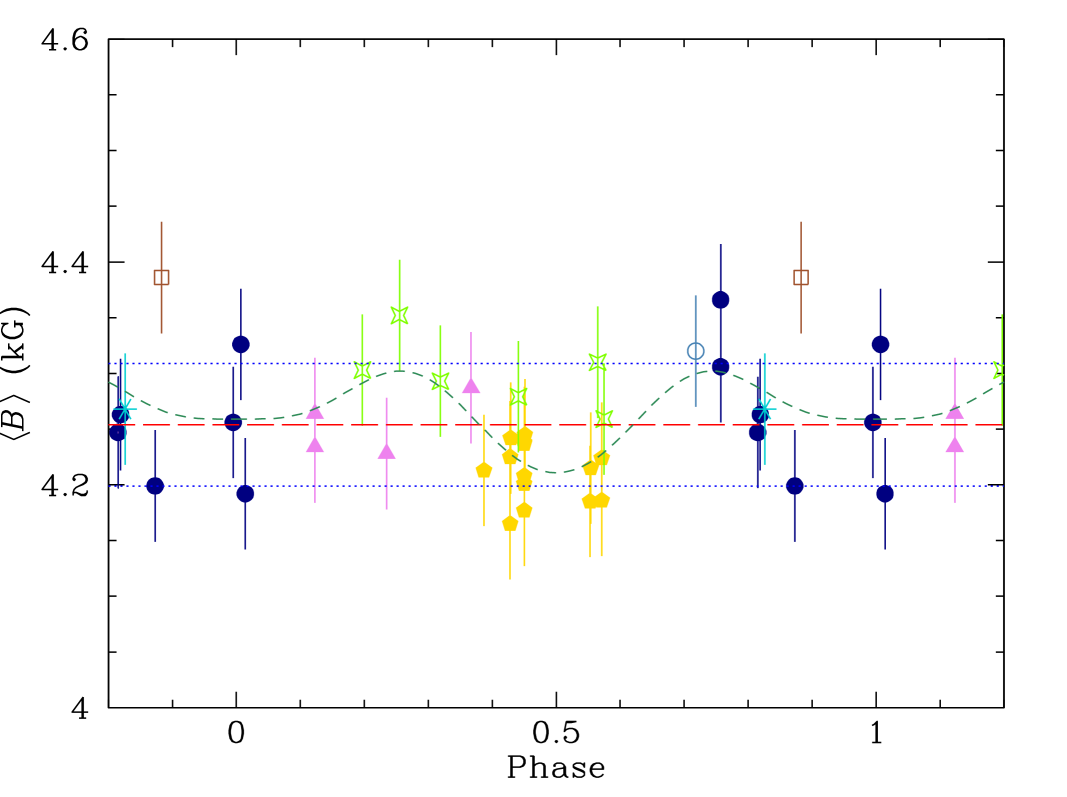
Figure 2: Mean magnetic field modulus of HD 965 against rotation phase. The different symbols identify the instrumental configuration from which the $\langle B\rangle$ value was obtained, as follows: filled circles (dark blue): CAT + CES LC; asterisk (turquoise): CAT + CES LC, lower resolution; open circle (steel blue): CAT + CES SC; open square (brown): OHP 1.52 m + AURELIE; filled triangles (violet): CFHT + Gecko (all previous symbols identical to Mathys 2017); four-pointed open stars (light greeen): UT2 + UVES; filled pentagons (yellow): 3.6 m + HARPS. The short-dashed line (green) corresponds to the superposition of low-order multipoles discussed in Sect. 4. The dotted lines (blue) correspond to $\pm 1$ standard deviation of the individual measurements about their average value (red dashed line).

The measurements of the mean magnetic field modulus $\langle B\rangle$ are also plotted against rotation phase, in Fig. 2. There is no apparent trend; the $\langle B\rangle$ values do not show any dependence on the observation phase. Furthermore, the scatter of these values is consistent with their estimated uncertainties: the average of our 34 measurements is $\langle B\rangle_{\rm av}=4254$ G, with a standard deviation of 55 G. This leads us to conclude that the mean field modulus of HD 965 is constant at the achieved precision level.

On the other hand, consideration of Fig. 2 suggests that the $\langle B\rangle$ measurements obtained from HARPS spectra may be slightly but systematically shifted downward, and those obtained from UVES spectra, shifted upward, with respect to the values obtained with the CES and Gecko. This may be indicative of some amount of systematic error of instrumental origin. However, the magnitude of the observed offset, a few tens of G, is small, at most of the same order as the random measurement uncertainties, so that one should be careful not to overinterpret it. It is also noteworthy that the highest $\langle B\rangle$ value was obtained from the only AURELIE observation. This again may arise from an instrumental effect, since AURELIE is known to be definitely subject to such effects (Mathys et al. 1997). However, no definitive conclusion can be drawn from consideration of a single measurement point.

In any event, whether the instrumental effects discussed above are actually present or not, their magnitude is small enough so that they do not question the conclusion that the mean magnetic field modulus of HD 965 does not show any significant variability.

One observable that shows prominent variability with the same period as $\langle B_{z}\rangle$ is the intensity of the Nd iii $\lambda\,6145$ line. While the high-resolution spectra from which we determined $\langle B\rangle$ cover a variety of spectral ranges, some of them very narrow, the Nd iii $\lambda\,6145$ line is present in all of them. The values of the equivalent width $W_{\lambda}$ of this line that we measured from these high-resolution spectra are plotted against the rotation phase in Fig. 4. They follow a very definite double-wave variation curve, with a primary maximum close to the phase of the negative extremum of the mean longitudinal magnetic field, and a secondary maximum near the phase of the positive extremum of $\langle B_{z}\rangle$. The observed variation of the equivalent width of the Nd iii $\lambda\,6145$ line in HD 965 represents an independent confirmation of the rotation period of this star.

As noted by Mathys (2017), the equivalent widths of the Fe lines do not show any variability, so that there is no indication of departures from uniformity in the distribution of this element over the stellar surface. The equivalent width and magnetic resolution of several of the Fe lines are of the same order as for the Nd iii $\lambda\,6145$ line: this represents a strong indication that the observed variations of the equivalent width of the latter reflect the inhomogeneous distribution of Nd over the stellar surface, not the occurrence of non-uniform magnetic desaturation.

Figure 3: Periodogram of the variations of the mean longitudinal magnetic field of HD 965. The ordinate is the reduced $\chi^{2}$ of a fit of the $\langle B_{z}\rangle$ measurements by a cosine wave, with the frequency given in abscissa.

4 Magnetic field characterisation

The observed variations of the mean longitudinal magnetic field of HD 965 can be well represented by a cosine wave. The best least-squares fit solution for $P_{\rm rot}=6030$ d is:

$$\langle B_{z}\rangle(\phi) = (-306\pm 14)$$ (4)

$$+ (911\pm 21)\,\cos\{2\pi\,[\phi-(0.501\pm 0.003)]\}$$

$$(\nu=62,\ \chi^{2}/\nu=7.9),$$

where the field strength is expressed in gauss, $\phi=({\rm HJD}-{\rm HJD}_{0})/P_{\rm rot}$ (mod 1) and the adopted value of ${\rm HJD}_{0}=2451000.0$ corresponds within the uncertainty of the phase to a negative extremum of the mean longitudinal magnetic field; $\nu$ is the number of degrees of freedom, and $\chi^{2}/\nu$, the reduced $\chi^{2}$ of the fit. The fitted curve is shown in Fig. 1; the $\mathrm{O}-\mathrm{C}$ differences between the individual measurements and this curve are also illustrated. The rather high value of $\chi^{2}/\nu$ may indicate that the uncertainty of some of the measurements is slightly underestimated, that there are some (small) systematic differences between the measurements of the different groups, or that the actual shape of the $\langle B_{z}\rangle$ variation curve departs somewhat from a cosine wave – or some combination of these effects. However, no mathematically significant contribution of the first harmonic was found. In particular, the $\langle B_{z}\rangle$ variation curve appears to be very nearly mirror-symmetric about the phases of its extrema.

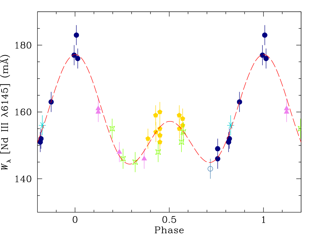
Figure 4: Equivalent width of the Nd iii $\lambda\,6145$ line against rotation phase. The symbols have the same meaning as in Fig. 2. The long-dashed line (red) is the best fit of the measurements by a cosine wave and its first harmonic. It has been included to guide the eye despite its lack of physical meaning.

The reversal of the sign of the mean longitudinal field over the rotation cycle indicates that both magnetic poles of the star come alternatively into sight. The constancy of the mean magnetic field modulus in a star of which both magnetic poles come alternatively into sight is unique (see Fig. 9 of Mathys 2017). Combined with the large amplitude and the sign reversal of the mean longtiudinal field, it sets a strong constraint on the geometrical structure of the magnetic field of HD 965.

In contrast with other extremely slowly rotating Ap stars that were recently studied, such as HD 18078 (Mathys et al. 2016) or HD 50169 (Mathys et al. 2019), neither the mean longitudinal magnetic field nor the mean magnetic field modulus of HD 965 show any hint of significant deviations of the geometrical structure of the large-scale magnetic field from axisymmetry. Accordingly, a simple axisymmetric model such as the superposition of collinear dipole, quadrupole, and octupole (Landstreet & Mathys 2000) may in principle be adequate to represent this structure. We computed such a model using a Python programme that is based on J. D. Landstreet’s Fldcurv code (e.g., Wade et al. 2006) and solves a non-linear least-squares minimisation problem, fitting both the $\langle B_{z}\rangle$ and $\langle B\rangle$ variation curves simultaneously. The best parameter values are $i=75.4^{\circ}\pm 0.8^{\circ}$, $\beta=37.2^{\circ}\pm 1.1^{\circ}$, $B_{\rm dipole}=(-5653\pm 119)$ G. $B_{\rm quadrupole}=(-281\pm 171)$ G. and $B_{\rm octupole}=(2872\pm 377)$ G. As usual, the angles $i$ (inclination of the rotation axis on the line of sight) and $\beta$ (angle between the rotation and magnetic axes) can be interchanged with no changes in the predicted variation curves. These curves are shown as dark green, short-dashed lines in Figs. 1 and 2. One should note the similarity of the model curve to the cosine best fit curve for the mean longitudinal magnetic field, and the fact that the amplitude of the model curve for the mean magnetic field modulus is lower than the standard deviation of the individual meaurements of this field moment about their mean. The quadrupolar component of the model is almost negligible. The two main components, a dipole and an octupole with opposite orientations, give a good approximation of a field that, in $\langle B_{z}\rangle$, appears essentially dipolar, but for which $\langle B\rangle$ indicates that the modulus of the field vector is nearly constant over the entire visible part of the stellar surface. However, while the adopted model provides a satisfactory representation of the observed variations, one cannot be sure that it is physically meaningful, and accordingly, the uncertainties given for the model parameters are only formal.

5 Discussion

With a rotation period of 6030 d, or 16.5 yr, HD 965 is only the third Ap star with a rotation period longer than 10 yr for which the value of this period has been determined exactly, and well sampled magnetic variation curves have been obtained.

Despite the extreme character of HD 965 in several respects (see Sect. 1), its magnetic field does not appear extraordinary in any way. Its most remarkable property is the lack of significant variability of $\langle B\rangle$ within the excellent precision of the measurements of this field moment (within 50 G). While large values of the ratio $q$ between the extrema of the mean magnetic field modulus are more frequently observed in slowly rotating Ap stars than in those that rotate faster (see Fig. 5 of Mathys 2017), this ratio is small in some of the long-period stars. HD 965 is becoming the longest-period star known to have $q\sim 1$. This does not make it exceptional in that respect, but rather results from the fact that among the slowly rotating Ap stars whose periods have been determined exactly, only two have longer periods. Once longer periods are determined for more stars, some of them will likely show low amplitude variability of $\langle B\rangle$.

The combination of $q\approx 1.0$ with a value $r=-0.50$ of the ratio of the smaller (in absolute value) to the larger (in absolute value) extremum of $\langle B_{z}\rangle$ is somewhat more remarkable, since large relative amplitudes of the mean magnetic field modulus tend to be found in stars for which both poles come alternately into view (see Fig. 9 of Mathys 2017). But it should not be regarded as a major anomaly; other stars in which both magnetic poles are seen show $\langle B\rangle$ variations of low relative amplitude.

The nearly constant value of the mean magnetic field modulus of HD 965, which averages at $\langle B\rangle_{\rm av}=4254$ G, is well below the value of 7.5 kG that seems to represent an upper limit to the field strength for those Ap stars with rotation periods longer than 150 d (Mathys et al. 1997; Mathys 2017). With a value of 0.18, the ratio of the rms longitudinal magnetic field (Bohlender et al. 1993), $\langle B_{z}\rangle_{\rm rms}=776$ G, to $\langle B\rangle_{\rm av}$, is also well within the typical range (see Fig. 8 of Mathys 2017).

Even though the modulus of the magnetic field vector must be mostly constant over the surface of HD 965, the distribution of the abundances of at least some elements (in particular, Nd) is markedly inhomogeneous. This suggests, perhaps not surprisingly, that the local orientation of the magnetic field must be more of a determining factor than its strength in the formation of chemical spots on the surfaces of Ap stars.

Elkin et al. (2005) suggested that the null results of the two attempts that were made to detect pulsations in HD 965 could possibly be attributed to the mostly equator-on aspect of the star at the epochs when the observations were performed. The phases of these observations can now be determined: 0.249 for the photometric study of Kurtz et al. (2003), and 0.319 for the high-resolution spectroscopic recordings of Elkin et al. (2005). Consideration of Fig. 1 confirms that both observations sampled primarily the part of the stellar surface close to the magnetic equator. Accordingly, it may be worth making a new attempt at detecting non-radial pulsations in HD 965 close to a magnetic extremum, when one of the magnetic poles, around which the pulsation amplitude is expected to be highest, is at maximum visibility. The next opportunity to do so will arise close to the forthcoming positive extremum of the mean longitudinal magnetic field, in the second half of 2022.