Chemo-dynamical properties of the Anticenter Stream: a surviving disc fossil from a past satellite interaction.

Abstract

Using Gaia DR2, we trace the Anticenter Stream (ACS) in various stellar populations across the sky and find that it is kinematically and spatially decoupled from the Monoceros Ring. Using stars from lamost and segue, we show that the ACS is systematically more metal-poor than Monoceros by $0.1$ dex with indications of a narrower metallicity spread. Furthermore, the ACS is predominantly populated of old stars ($\sim 10\,\rm{Gyr}$), whereas Monoceros has a pronounced tail of younger stars ($6-10\,\rm{Gyr}$) as revealed by their cumulative age distributions. Put togehter, all of this evidence support predictions from simulations of the interaction of the Sagittarius dwarf with the Milky Way, which argue that the Anticenter Stream (ACS) is the remains of a tidal tail of the Galaxy excited during Sgr’s first pericentric passage after it crossed the virial radius, whereas Monoceros consists of the composite stellar populations excited during the more extended phases of the interaction. We suggest that the ACS can be used to constrain the Galactic potential, particularly its flattening, setting strong limits on the existence of a dark disc. Importantly, the ACS can be viewed as a stand-alone fossil of the chemical enrichment history of the Galactic disc.

1 Introduction

Signs of vertical disc perturbations to the disc have been known from the distribution of the neutral hydrogen gas since the 1950s (Burke, 1957). In recent years, interest in disc quakes - particularly in the stellar component - has been reinvigorated with the discovery of spatial and kinematic North/South asymmetries around the solar neighbourhood (Widrow et al., 2012; Williams et al., 2013; Carlin et al., 2013; Carrillo et al., 2018; Schönrich & Dehnen, 2018). As revealed by star count studies, these asymmetries take their most dramatic form in the outer edge of the Galaxy where the self-gravity of the disc is at its weakest. Amongst the various tributaries of the Galactic Anticenter, we count the Monoceros Ring (Newberg et al., 2002; Slater et al., 2014) and its substructured content, namely the Anticenter Stream (ACS) and Eastern Banded Structure (Grillmair, 2006) that most visibly stand out in main-sequence (MS) and main-sequence turn-off (MSTO) star counts. Although initially thought to be part of the remains of a torn-apart accreted dwarf galaxy (Peñarrubia et al., 2005), recent theoretical (Gómez et al., 2016; Laporte et al., 2018, 2019a) and observational studies favour an excited disc origin for these structures as supported by the kinematics (de Boer et al., 2018; Deason et al., 2018) and stellar populations (e.g. see Price-Whelan et al., 2015; Sheffield et al., 2018) with manifestly disc-like properties.

Recently, Laporte et al. (2019a) suggested a re-interpretation of the Anticenter Stream as the remnant of a tidal tail (“feather”) excited by the Sgr dwarf galaxy shortly after virial radius crossing. A falsifiable predictions of this scenario is that the stellar populations of Monoceros and the ACS should show differences in metallicity and age distributions. In particular, because the ACS got excited through resonant processes with the reaction of the Milky Way’s dark matter halo with Sgr, it must have decoupled itself from the rest of the disc and should hold predominantly old stars and very few young ones. With the current synergy between legacy spectroscopic surveys (segue, lamost, apogee) and the second data release from Gaia, it is now possible to dissect the Anticenter to much greater detail and test the tidal tail remnant hypothesis with chemistry and dynamics. This is the aim of the following contribution. In Section 2, we discuss our target selection and masks in the Monoceros Complex and cross-matches to the aforementioned spectroscopic surveys. In Section 3, we dissect the Monoceros Ring and ACS in metallicity, age and abundance. We discuss our main findings and conclude in Sections 4 and 5.

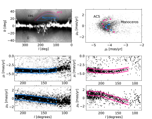
Figure 1: Top left: MS/MSTO map of the Anticenter in Galactic coordinates $(l,b)$ with selected spatial footprints for the ACS and Monoceros Ring. ACS sits above the Monoceros Ring as a long collimated thin structure. Top right: Latitudinal against longitudinal proper motions for RC stars. The median proper motion tracks for the ACS and Monoceros are shown by the magenta and blue dots. Middle left: Normalised histogram for longitudinal proper motions $\mu_{l}$ as a function of $l$ for “ACS field” stars. Proper motion masks and median $\mu_{l}$ within them are shown in magenta. Middle right: Normalised histogram for longitudinal proper motions $\mu_{l}$ as a function $l$ for “Monoceros field” stars. Proper motion masks and median $\mu_{l}$ within them are shown in blue. Bottom left: Normalised histogram for latitudinal proper motions $\mu_{b}$ as a function of $l$ for “ACS field” stars. Note that this mask avoids the contamination from Monoceros situated below $\mu_{b}\sim 1\rm{mas/yr}$ for $l>200$ as the ACS and Monoceros overlaps spatially in those zones due to its reconnection with the midplane, yet show remarkably different kinematics. Proper motion masks and median $\mu_{b}$ within them are shown in magenta. Bottom right: Normalised histogram for latitudinal proper motions $\mu_{b}$ as a function of $l$ for “Monoceros field” stars. Proper motion masks and median $\mu_{b}$ within them are shown in blue.

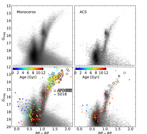
Figure 2: Top panels: CMDs for Monoceros and ACS fields (left and right panels respectively). The kinematic and spatial selection picks up a well defined RGB, RC all the way down to a MSTO/MS. The excess of blue stars may be a population of blue stragglers (BS). Bottom panels: Stars identified in the Sanders & Das (2018) catalog are shown as points colour-coded as a function of age. apogee cross-matched stars are shown as open white-filled black circles.

2 Target selection

For our study, we make use of the GDR2 proper motions and parallaxes to identify the likely ACS and Monoceros members. We correct magnitudes and colours for extinction by using the Schlegel et al. (1998) dustmap and assuming $A_{X}=A_{0}k_{X}$, where $X$ designates the passband and $k_{X}$ the first extinction coefficient of the relation used by Danielski et al. (2018) adapated to the Gaia passabands assuming that $A_{0}=3.1E(B-V)$ (Gaia Collaboration et al., 2018). To guide our initial spatial search, we begin by selecting the main-sequence/main-sequence turn-off (MS/MSTO) by requiring $0.5<BP-RP<0.8$ and $18<G_{0}<20$ and $\varpi<0.1$. We then convert the coordinates to a new system approximately aligned with the Anticenter by rotating the celestial equator to the great circle with a pole at (l,b) = (325.00, 67.4722). The ACS and Monoceros stars are drawn from the spatial masks shown in Galactic coordinates in the top left panel of Figure 1. Moreover, in the top right panel of the Figure, using the Red Clump (RC) stars (selected with the cuts $15.5<G_{0}<15.9$, $1.0<BP-RP<1.1$ and $\varpi<0.1$), we demonstrate that the Monoceros Ring and the Anticenter stream not only have distinct spatial distributions but also differ kinematically. This is evidenced by the bifurcating pattern in $(\mu_{l},\mu_{b})$ space for which we also present median proper motion tracks in magenta (blue) for the ACS (Monoceros) respectively. This two-horned structure confirms some of the earlier suggestions of de Boer et al. (2018) based on the Gaia DR1-SDSS astrometric analysis.

We proceed by using Gaia DR2 to identify high-fidelity candidate stars belonging to the ACS and the Monoceros regions. We make use of the parallax cut $\varpi<0.1$ as well as the proper motion masks shown in Figure 1. The two bottom rows of the Figure give column-nornalized RC density in the space of $\mu_{b}$ and $\mu_{l}$ proper motions as a function of Galactic longitude $l$ for Monoceros (ACS) in the left (right). The proper motion masks - highlighted by the magenta and blue boxes respectively - are chosen to include the highest-density signal at each $l$. Figure 2 presents CMDs for both fields and only displays stars that have passed the proper motion and parallax cuts described above. Readily identifiable in the Figure are several familiar stellar populations: MS/MSTO, RC and red giant branch (RGB), thus confirming that our selection picks up bona-fide stars associated with the two individual well-defined structures. Moreover, note that the Hess diagram of the Monoceros Ring is much broader compared to the ACS, which signals a larger mix of metallicities and ages and possibly line-of-sight distances.

3 Chemical and age decomposition of Monoceros and the ACS

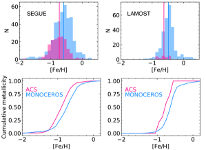
Figure 3: Left: Metallicity distribution for stars cross-matched with segue for the ACS and Monoceros Ring in magenta and blue respectively. The median and spreads in metallicity $([\rm{Fe/H}],\sigma[\rm{Fe/H}])$ are $(-0.73,0.26)$ and $(-0.59,0.32)$ for the ACS and Monoceros Ring respectively. Right: Metallicity distribution for stars cross-matched with sc lamost for the ACS and Monoceros Ring in magenta and blue respectively. The median and spreads in metallicity $([\rm{Fe/H}],\sigma[\rm{Fe/H}])$ are $(-0.62,0.14)$ and $(-0.48,0.22)$ for the ACS and Monoceros Ring respectively.

3.1 Metallicity distributions

The lamost DR4 survey (Luo et al., 2015) provides a good coverage of the Anticenter region, with a large number of spectra measured across both structures without a strong metallicity bias (see e.g. Yanny et al., 2009). segue fares similarly well and has also the advantage of reaching down to the main-sequence and the turn-off at larger distances. This is particularly advantageous to analyse differences in age distributions between Monoceros and the ACS for which the MSTO is sensitive to. Note however that segue includes a sub-dominant target category (F sub-dwarfs) biased against metal-richer stars. Furthermore, in order to avoid any source of confusion we only analyse stars in the range $115<l<175$ as these regions separate most clearly between the ACS and Monoceros fields both spatially and kinematically (see Figure 1). We select spectra with signal-to-noise ratios of SNR$\geq 10$ for lamost a SNR$\geq 20$ for segue. Figure 3 shows metallicity distributions for the likely Monoceros and the ACS members from our cross-matches with lamost and segue. Although the numbers differ from one survey to another, both spectroscopic samples reveal similar systematic trends. The median metallicity of the ACS is consistently lower than that of Monoceros by some $\Delta[Fe/H]\sim 0.1\,\rm{dex}$.

3.2 Age distributions

To study the star-formation histories of the two structures, we cross-match the candidate stars identified above with the catalog of stellar ages computed by Sanders & Das (2018). Figure 4 shows the cumulative age distributions for the ACS and Monoceros regions . The difference between the two structures are remarkable, with the ACS being predominantly composed of older stars $\tau_{{\rm ACS}}>10\,\rm{Gyr}$ whereas Monoceros possessing a more steady, gradual star-formation history. We checked that there was no correlation between age and metallicity in our subset of Sanders & Das (2018) cross-matched stars and that the distances are consistent with the structures ($d\sim 10\,\rm{kpc}$). In the encounter scenario (see Laporte et al., 2019a), the ACS is a group of stars located in a tidal tail of the Galactic disc which gets decoupled from the rest of the disc and propelled to larger heights from midplane after first pericentric passage of a massive satellite (e.g. Sgr), whereas Monoceros consists of stellar populations in the flared and corrugated outer disc which was gradually built up through a succession of encounters, allowing it to replenish itself with younger stars as the star formation proceeded.

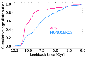
Figure 4: Cumulative age distribution of stars cross-matched with the Sanders & Das (2018) catalog. The ACS shows a rapid increase in its cumulative distribution with about 80% of the stars being older than 10 Gyr, whereas the Monoceros Ring shows a much more steady formation of stars.

Figure 5 presents a spatial median age map of the Anticenter region. We find that the ACS is systematically older than the Monoceros Ring which hosts plenty of intermediate age stars (5-9 Gyr). Note a sharp age boundary between the two structures matching the location of the density transition (c.f. Figure 1).

Figure 5: Spatial map of star median ages. Footprints of Monoceros and the ACS are shown in blue and magenta respectively. weave high-resolution footprint (Jin et al. in prep) is overlaid in black open circles.

3.3 apogee chemical abundances for the ACS and Monoceros

Despite its pencil-beam nature, the apogee survey (Majewski et al., 2017) covers parts of both the ACS and the Monoceros Ring. This allows us to acquire alpha-element abundances for our candidate stars through cross-matching catalogs. This gives us a few candidate stars which fall within the RGB/RC as shown in Figure 2. In Figure 6, we show the locations of our apogee cross-matched stars in the the space of $([Mg/Fe],[Fe/H])$. Not surprisingly, these stars belong to the low-$\alpha$ sequence with $0<[Mg/Fe]<0.15$ and low metallicity $-0.8<[Fe/H]<0.3$, commonly known as the chemical “thin disc”, which confirms that the ACS and Monoceros Ring are not tidal debris from accretion events but truly extensions of the outer disc. This is not surprising as other/similar structures of the Anticenter have also recently been confirmed to be chemical thin-disc material through abundance measurements (e.g. see Bergemann et al., 2018) and stellar populations content (Price-Whelan et al., 2015; Sheffield et al., 2018).

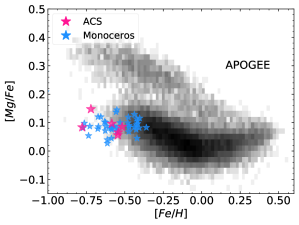
Figure 6: Magnesium abundance versus metallicity of stars in ACS and Monoceros within the proper motion masks defined in Section 1 (magenta and blue star symbols respectively). Despite the pencil beam nature of the apogee survey, a few stars associated with Monoceros and the ACS are picked up and show a clear low-alpha abundance sequence consistent with the chemical “thin disc”. The full apogee disc $[Mg/Fe]$ vs $[Fe/H]$ map is displayed in grey-scale for comparison.

4 Discussion

By using a combination of astrometric, photometric and spectroscopic information, we were able to dissect the Monoceros Ring and the ACS in the space of kinematics, metallicities, $\alpha$-abundances and ages. This allowed us to explore and confirm a falsifiable prediction for their respective formation mechanisms as presented in (Laporte et al., 2019a), namely that the ACS is the remnant tidal tail of the MW disc which formed through a resonant interaction with the Sgr dwarf galaxy. The ACS was kicked up shortly after the dwarf’s crossing of the Galaxy’s virial radius during one of the first pericentric passages. The ACS excitation resulted in a strong decoupling from the Galactic midplane, leading to a sudden shutdown of star formation as compared to the rest of the disc. This yielded the observed striking difference in the cumulative age distributions between the Monoceros and the ACS.

We note that several structures in the outer disc have also been identified. These include the EBS (Grillmair, 2006) and the more distant TriAnd clouds (Rocha-Pinto et al., 2004). A similar analysis could in principle be pursued, in particular for the TriAnd, which lies at a larger distance. This is particularly interesting as these structures may represent a fossil record of the formation history of the outer disc. Via modelling of such structures one can hope to time the impact events, putting strong constraints on the orbital mass-loss history of the Sgr dwarf galaxy. Our analysis argues that it may be possible to use chemistry and age dating important events in the lifetime of the Galactic disc. The decoupled nature of the structures analysised here - the ACS and the Monoceros - is of particular interest for chemo-dynamical models of the Galaxy (e.g. Chiappini et al., 1997; Schönrich & Binney, 2009).

Given the disc nature of the ACS, and the relatively simple dynamics of “feathers” (Laporte et al., 2019a), this structure may also be used for constraining the flattening of the Galactic potential at large radii, thus setting strong limits on alternative dark matter models or the existence of a dark disc Read et al. (2008), however this is beyond the scope of this contribution and will be presented elsewhere.

5 Conclusion

In this work, we took full advantage of the synergy between Gaia DR2, segue, lamost and apogee to show that:

1. The ACS and Monoceros Ring are spatially and kinematically separate structures.

2. The ACS is on average more metal-poor than the Monoceros Ring, by $\geq 0.1\,\rm{dex}$, with hints of a smaller spread in metallicity (though this could perhaps be accounted by distance spreads too).

3. The ACS and Monoceros Ring are both part of the chemically thin-disc due to their low magnesium abundances, with $0.0<[Mg/Fe]<0.15$.

4. The ACS has predominantly old stellar populations with 80% of the having an age $>10\,\rm{Gyr}$. This taken with its physical and kinematic decoupling from the rest of the disc, supports the hypothesis that this group of stars is a “feather”, i.e. the remnant of a tidal tail excited by a satellite encounter such as that with the Sgr dwarf described in Laporte et al. (2019a). In this model, the ACS is extracted from the disc during the dwarf’s first passage after virial radius crossing, and no longer forms stars.

5. The Monoceros Ring shows a steady cumulative age distribution suggesting that it belongs to main body of the disc which has been gradually flared and corrugated as a result of the multiple passages of Sgr and populated by stars of different ages as star formation continued.

As an outlook into the future, surveys such as weave, sdss v, 4most and psf will pave the road to a full coverage of the Anticenter. These surveys will not only provide radial velocities for a full characterisation of the the phase-plane spiral in the outer disc as predicted by numerical models of the interaction of Sgr with the Milky Way (Laporte et al., 2018, 2019b) but will also allow for a more detailed chemical dissection of the Anticenter. In particular, the latter will provide a window into the fossil record of the Galactic disc’s formation.

References

- Bergemann et al. (2018) Bergemann M., Sesar B., Cohen J. G., Serenelli A. M., Sheffield A., Li T. S., 2018, Nature, 555, 334
- Burke (1957) Burke B. F., 1957, AJ, 62, 90
- Carlin et al. (2013) Carlin J. L., DeLaunay J., Newberg H. J., Deng L., Gole D., Grabowski K., 2013, ApJL, 777, L5
- Carrillo et al. (2018) Carrillo I., Minchev I., Kordopatis G., Steinmetz M., Binney J., Anders F., Bienaymé O., Bland-Hawthorn J., Famaey 2018, MNRAS, 475, 2679
- Chiappini et al. (1997) Chiappini C., Matteucci F., Gratton R., 1997, ApJ, 477, 765
- Danielski et al. (2018) Danielski C., Babusiaux C., Ruiz-Dern L., Sartoretti P., Arenou F., 2018, AAP, 614, A19
- de Boer et al. (2018) de Boer T. J. L., Belokurov V., Koposov S. E., 2018, MNRAS, 473, 647
- Deason et al. (2018) Deason A. J., Belokurov V., Koposov S. E., 2018, MNRAS, 473, 2428
- Gaia Collaboration et al. (2018) Gaia Collaboration Babusiaux C., van Leeuwen F., Barstow M. A., Jordi C., Vallenari A., Bossini D., Bressan A., Cantat-Gaudin T., van Leeuwen M., 2018, AAP, 616, A10
- Gómez et al. (2016) Gómez F. A., White S. D. M., Marinacci F., Slater C. T., Grand R. J. J., 2016, MNRAS, 456, 2779
- Grillmair (2006) Grillmair C. J., 2006, ApJL, 651, L29
- Hunter (2007) Hunter J. D., 2007, Computing In Science & Engineering, 9, 90
- Jones et al. (01 ) Jones E., Oliphant T., Peterson P., et al.,, 2001–, SciPy: Open source scientific tools for Python
- Laporte et al. (2018) Laporte C. F. P., Johnston K. V., Gómez F. A., Garavito-Camargo N., Besla G., 2018, MNRAS, 481, 286
- Laporte et al. (2019a) Laporte C. F. P., Johnston K. V., Tzanidakis A., 2019, MNRAS, 483, 1427
- Laporte et al. (2019b) Laporte C. F. P., Minchev I., Johnston K. V., Gómez F. A., 2019, MNRAS, 485, 3134
- Luo et al. (2015) Luo A. L., Zhao Y.-H., Zhao G., Deng L.-C., Liu X.-W., Jing Y.-P., Wang G., Zhang H.-T., Shi J.-R., Cui X.-Q., 2015, Research in Astronomy and Astrophysics, 15, 1095
- Majewski et al. (2017) Majewski S. R., Schiavon R. P., Frinchaboy P. M., Allende Prieto C., Barkhouser R., 2017, AJ, 154, 94
- Newberg et al. (2002) Newberg H. J., Yanny B., Rockosi C., Grebel E. K., Rix H.-W., Brinkmann J., 2002, ApJ, 569, 245
- Peñarrubia et al. (2005) Peñarrubia J., Martínez-Delgado D., Rix H. W., Gómez-Flechoso M. A., 2005, ApJ, 626, 128
- Price-Whelan et al. (2015) Price-Whelan A. M., Johnston K. V., Sheffield A. A., Laporte C. F. P., Sesar B., 2015, MNRAS, 452, 676
- Read et al. (2008) Read J. I., Lake G., Agertz O., Debattista V. P., 2008, MNRAS, 389, 1041
- Rocha-Pinto et al. (2004) Rocha-Pinto H. J., Majewski S. R., Skrutskie M. F., Crane J. D., Patterson R. J., 2004, ApJ, 615, 732
- Sanders & Das (2018) Sanders J. L., Das P., 2018, MNRAS, 481, 4093
- Schlegel et al. (1998) Schlegel D. J., Finkbeiner D. P., Davis M., 1998, ApJ, 500, 525
- Schönrich & Binney (2009) Schönrich R., Binney J., 2009, MNRAS, 396, 203
- Schönrich & Dehnen (2018) Schönrich R., Dehnen W., 2018, MNRAS, 478, 3809
- Sheffield et al. (2018) Sheffield A. A., Price-Whelan A. M., Tzanidakis A., Johnston K. V., Laporte C. F. P., Sesar B., 2018, ApJ, 854, 47
- Slater et al. (2014) Slater C. T., Bell E. F., Schlafly E. F., Morganson E., Martin N. F., Rix H.-W., Peñarrubia J., 2014, ApJ, 791, 9
- Van Der Walt et al. (2011) Van Der Walt S., Colbert S. C., Varoquaux G., 2011, Computing in Science & Engineering, 13, 22
- Widrow et al. (2012) Widrow L. M., Gardner S., Yanny B., Dodelson S., Chen H.-Y., 2012, ApJL, 750, L41
- Williams et al. (2013) Williams M. E. K., Steinmetz M., Binney J., Siebert A., Enke H., Famaey B., 2013, MNRAS, 436, 101
- Yanny et al. (2009) Yanny B., Rockosi C., Newberg H. J., Knapp G. R., Adelman-McCarthy J. K., Alcorn B., 2009, AJ, 137, 4377