Diagrams for nonabelian Hodge spaces on the affine line

Abstract.

In this announcement a diagram will be defined for each nonabelian Hodge space on the affine line.

1. Introduction

In a previous paper ([3] Apx. C), a diagram was defined for each algebraic connection on a vector bundle on the affine line, under the condition that the connection was untwisted at infinity (i.e. had unramified irregular type). In that case the diagram was a graph (or a “doubled quiver”). It is known that such a connection determines a triple of complex algebraic moduli spaces $\mathcal{M}_{\text{\rm DR}},\mathcal{M}_{\text{\rm Dol}},\mathcal{M}_{\text{\rm B}}$, which are algebraically distinct yet naturally diffeomorphic. In other words the connection determines a single nonabelian Hodge space $\mathfrak{M},$ with a triple of distinct algebraic structures. Hence this gives a way to attach a diagram to a class of nonabelian Hodge spaces. The simplest examples of such graphs match up with the affine Dynkin diagrams corresponding to the Okamoto Weyl group symmetries of the Painlevé equations (corresponding to some of the H3 surfaces, i.e. the spaces $\mathfrak{M}$ of real dimension four). More background and motivation related to integrable systems and isomonodromy is recounted in [6].

The purpose of this note is to extend this story by defining a diagram for any algebraic connection on a vector bundle on the affine line, i.e. for any nonabelian Hodge space attached to the affine line. One can show using the Fourier–Laplace transform that any moduli space $\mathcal{M}_{\text{\rm DR}}$ of meromorphic connections on a smooth affine curve of genus zero is isomorphic to one on the affine line (i.e. with just one puncture), and this is expected to hold for the full nonabelian Hodge triple. It is thus hoped that these diagrams serve a useful purpose in the classification of nonabelian Hodge spaces (and this is certainly the case in the examples considered in [3, 4, 5]).

2. The construction

Let $\Sigma=\mathbb{P}^{1}(\mathbb{C})$ and fix a point $p=\infty\in\Sigma$ so that $\Sigma^{\circ}=\Sigma\setminus p$ is the affine line. The diagram of an algebraic connection $(E,\nabla)\to\Sigma^{\circ}$ is determined by its formal isomorphism class at $\infty$. This formal class is equivalent to the irregular class plus the formal monodromy conjugacy classes, as follows.

Let $\partial$ be the circle of real oriented directions at $p$. Recall that the exponential local system $\mathcal{I}$ is a covering space $\pi:\mathcal{I}\to\partial$, consisting of a disjoint union of circles $\langle q\rangle$ each of which is a finite cover of $\partial$. (This notation is from [8, 7] where further discussion and references may be found). Deligne’s way of stating the Hukuhara–Turritin–Levelt formal classification of connections is as follows:

Theorem 1 ([15] Thm 2.3).

The category of connections on vector bundles on the formal punctured disk at $p$ is equivalent to the category of $\mathcal{I}$-graded local systems $V^{0}\to\partial$ of finite dimensional complex vector spaces.

Such a graded local system $V^{0}$ is the same thing as a local system (of finite dimensional complex vector spaces) on the topological space $\mathcal{I}$, having compact support (in the sense that it has rank zero on all but a finite number of component circles of $\mathcal{I}$).

By definition the irregular class of a connection is the map $\Theta:\pi_{0}(\mathcal{I})\to\mathbb{N}$ taking the rank of $V^{0}$ on each circle ([8] §3.5). In down to earth terms the circles $\langle q\rangle$ correspond to the exponential factors $e^{q}$ of the corresponding connection, so fixing the irregular class amounts to fixing the exponential factors plus their integer multiplicities. Thus an irregular class can be written as a formal sum

$$\Theta=n_{1}\langle q_{1}\rangle+\cdots+n_{m}\langle q_{m}\rangle$$

of a finite number of distinct circles $\langle q_{i}\rangle$, with integer multiplicities $n_{i}=\Theta(q_{i})\geq 1$.

Now a local system of rank $n$ on a circle $\langle q\rangle$ is a very simple object, and is classified by the conjugacy class in ${\mathop{\rm GL}}_{n}(\mathbb{C})$ of its monodromy (in a positive sense once around the circle). Thus the graded/formal local system $V^{0}$ determines conjugacy classes

$$\mathcal{C}=(\mathcal{C}_{1},\ldots,\mathcal{C}_{m}),\qquad\mathcal{C}_{i}\subset{\mathop{\rm GL}}_{n_{i}}(\mathbb{C})$$

where $\mathcal{C}_{i}$ is the class of the monodromy of the local system on the circle $\langle q_{i}\rangle$.

Now there is a well-known method due to Kraft–Procesi and others of attaching a graph $L$ (a type $A$ Dynkin graph) to a marked conjugacy class in ${\mathop{\rm GL}}_{n}(\mathbb{C})$. It is reviewed in [5] Defn 9.2. Moreover the graph is independent of the marking if the marking is chosen to be minimal, in the sense of [5] Defn 9.2. The number of nodes of $L$ is the degree of a minimal polynomial of any element of the class. Thus $V^{0}$ determines legs $L_{1},\ldots,L_{m}$, where $L_{i}$ is the type $A$ Dynkin graph determined by a minimal marking of the class $\mathcal{C}_{i}$.

The next step is to define the core diagram $\Gamma$. For this first recall (e.g. from [7]) that:

1) For any circle $\langle q\rangle\subset\mathcal{I}$ the ramification degree $\mathop{\rm ram}(q)$ is the degree of the covering map $\pi:\langle q\rangle\to\partial$,

2) The set of points of maximal decay is a discrete subset ${\includegraphics[height=8.61108pt]{apple3}}{}\subset\mathcal{I}$. It consists of a finite subset ${\includegraphics[height=8.61108pt]{apple3}}(q)\subset\langle q\rangle$ in each circle, where the function $e^{q}$ has maximal decay,

3) The size of the set ${\includegraphics[height=8.61108pt]{apple3}}(q)$ is called the irregularity $\text{\rm Irr}(q)$ of the irregular class $\langle q\rangle$ (and is zero if and only if $q=0$). For an arbitrary class $\Theta=\sum n_{i}\langle q_{i}\rangle$ the irregularity is $\text{\rm Irr}(\Theta)=\sum n_{i}\text{\rm Irr}(q_{i})$,

4) For any pair of circles $\langle q_{1}\rangle,\langle q_{2}\rangle$ the irregular class $\operatorname{Hom}(\langle q_{1}\rangle,\langle q_{2}\rangle)$ is well-defined (the definition is straightforward if one thinks in terms of corresponding graded local systems).

Now the core diagram $\Gamma$ is defined as follows:

$\bullet$ $\Gamma$ has $m$ nodes, labelled by the circles $\langle q_{1}\rangle,\ldots,\langle q_{m}\rangle$,

$\bullet$ If $i\neq j$ then the number of arrows from $\langle q_{i}\rangle$ to $\langle q_{j}\rangle$ is given by

(1) $$B_{ij}=A_{ij}-\beta_{i}\beta_{j}$$

where $\beta_{i}=\mathop{\rm ram}(q_{i}),A_{ij}=\text{\rm Irr}(\operatorname{Hom}(\langle q_{i}\rangle,\langle q_{j}\rangle))$,

$\bullet$ If $i=j$ the number of arrows from $\langle q_{i}\rangle$ to $\langle q_{i}\rangle$ (oriented loops) is

(2) $$B_{ii}=A_{ii}-\beta_{i}^{2}+1.$$

Definition 2.

The diagram $\mathchoice{\accentset{\displaystyle\text{\smash{\raisebox{-5.59721pt}{$\widehatsym$}}}}{\Gamma}}{\accentset{\textstyle\text{\smash{\raisebox{-5.59721pt}{$\widehatsym$}}}}{\Gamma}}{\accentset{\scriptstyle\text{\smash{\raisebox{-3.91806pt}{$\widehatsym$}}}}{\Gamma}}{\accentset{\scriptscriptstyle\text{\smash{\raisebox{-2.7986pt}{$\widehatsym$}}}}{\Gamma}}$ of $(\Theta,\mathcal{C})$ is obtained by gluing the end node of the leg $L_{i}$ to the node $\langle q_{i}\rangle$ of the core diagram $\Gamma$, for $i=1,\ldots,m$.

As usual (when drawing diagrams) a pair of oppositely oriented arrows is identified with a single unoriented edge. In particular a pair of oriented loops is the same thing as a single (unoriented) edge loop. One can show (e.g. using the symplectic results of [8]) that the integer $A_{ii}-\beta_{i}^{2}+1$ is always even, and so all the diagrams here only involve unoriented edges (it is clear that $B_{ij}=B_{ji}$). It should be noted that we call this a diagram, and not a graph, since some of the edges may have negative multiplicity. (The negative edges will be indicated by dashed lines in figures.) The meaning of a negative edge is that one has more relations than linear maps—the diagram arises since there are explicit matrix presentations of the wild character varieties, many of which date back to Birkhoff (cf. the history discussed in [7]). It is something of a surprise that there are (lots of) perfectly good moduli spaces whose diagrams have negative edges.

The untwisted case considered in [3] is the case where each $\beta_{i}=1$, so that $\langle q_{i}\rangle\to\partial$ is a trivial (degree one) cover. In this case each $q_{i}$ can be identified with a polynomial in $x$ with zero constant term (where $x$ is a coordinate on $\mathbb{A}^{1}=\mathbb{P}^{1}\setminus\infty$). In this case $\operatorname{End}(\langle q_{i}\rangle)=\langle 0\rangle$ so that $A_{ii}=0$ and so there are no edge loops. Further $\operatorname{Hom}(\langle q_{i}\rangle,\langle q_{j}\rangle)=\langle q_{j}-q_{i}\rangle$ is again unramified, and its irregularity is just the degree of the polynomial $q_{j}-q_{i}$, so that

(3) $$A_{ij}-\beta_{i}\beta_{j}=\deg(q_{i}-q_{j})-1.$$

It follows that the core diagram coincides with the graph $\Gamma$ defined in [3] Apx C. The irregular type $\sum A_{i}dz/z^{k-i}$ considered there is $dQ$ where $Q$ is the diagonal matrix with entries given by the $q_{i}$, written in the coordinate $z=1/x$. The simple expression $\deg(q_{i}-q_{j})-1$ for the edge multiplicities of this graph appears in [12] §3.3.

2.1. Adding some tame singularities

Here is how to extend this construction to the case where a finite number of tame singularities on $\mathbb{A}^{1}$ are included as well. (This is similar to the procedure for adding tame singularities at finite distance in [3, 4, 5]). As mentioned in the introduction, this case (and any other case on $\mathbb{P}^{1}$) can be reduced to the case already considered above via Fourier–Laplace.

Let $n=\operatorname{\mathop{\rm rk}}(E)=\operatorname{\mathop{\rm rk}}(V^{0})=\sum_{1}^{m}n_{i}\beta_{i}$ be the rank of the irregular class $\Theta$ considered above. Choose points $a_{1},\ldots,a_{k}\in\mathbb{A}^{1}(\mathbb{C})$, and fix a tame formal class at each point. This is the same as fixing conjugacy classes $\mathchoice{\accentset{\displaystyle\text{\smash{\raisebox{-5.59721pt}{$\widehatsym$}}}}{\mathcal{C}}}{\accentset{\textstyle\text{\smash{\raisebox{-5.59721pt}{$\widehatsym$}}}}{\mathcal{C}}}{\accentset{\scriptstyle\text{\smash{\raisebox{-3.91806pt}{$\widehatsym$}}}}{\mathcal{C}}}{\accentset{\scriptscriptstyle\text{\smash{\raisebox{-2.7986pt}{$\widehatsym$}}}}{\mathcal{C}}}_{1},\ldots,\mathchoice{\accentset{\displaystyle\text{\smash{\raisebox{-5.59721pt}{$\widehatsym$}}}}{\mathcal{C}}}{\accentset{\textstyle\text{\smash{\raisebox{-5.59721pt}{$\widehatsym$}}}}{\mathcal{C}}}{\accentset{\scriptstyle\text{\smash{\raisebox{-3.91806pt}{$\widehatsym$}}}}{\mathcal{C}}}{\accentset{\scriptscriptstyle\text{\smash{\raisebox{-2.7986pt}{$\widehatsym$}}}}{\mathcal{C}}}_{k}\subset{\mathop{\rm GL}}_{n}(\mathbb{C})$, i.e. the local monodromy conjugacy classes. (This is the same as fixing the isomorphism class of a graded local system at each point, but graded entirely by the corresponding tame circle $\langle 0\rangle$ with multiplicity $n$).

Let $\mathchoice{\accentset{\displaystyle\text{\smash{\raisebox{-5.59721pt}{$\widehatsym$}}}}{L}}{\accentset{\textstyle\text{\smash{\raisebox{-5.59721pt}{$\widehatsym$}}}}{L}}{\accentset{\scriptstyle\text{\smash{\raisebox{-3.91806pt}{$\widehatsym$}}}}{L}}{\accentset{\scriptscriptstyle\text{\smash{\raisebox{-2.7986pt}{$\widehatsym$}}}}{L}}_{i}$ be the leg determined by a minimal marking of $\mathchoice{\accentset{\displaystyle\text{\smash{\raisebox{-5.59721pt}{$\widehatsym$}}}}{\mathcal{C}}}{\accentset{\textstyle\text{\smash{\raisebox{-5.59721pt}{$\widehatsym$}}}}{\mathcal{C}}}{\accentset{\scriptstyle\text{\smash{\raisebox{-3.91806pt}{$\widehatsym$}}}}{\mathcal{C}}}{\accentset{\scriptscriptstyle\text{\smash{\raisebox{-2.7986pt}{$\widehatsym$}}}}{\mathcal{C}}}_{i}$ (in the sense of [5] Defn 9.2). Assuming each conjugacy class is non-central, each $\mathchoice{\accentset{\displaystyle\text{\smash{\raisebox{-5.59721pt}{$\widehatsym$}}}}{L}}{\accentset{\textstyle\text{\smash{\raisebox{-5.59721pt}{$\widehatsym$}}}}{L}}{\accentset{\scriptstyle\text{\smash{\raisebox{-3.91806pt}{$\widehatsym$}}}}{L}}{\accentset{\scriptscriptstyle\text{\smash{\raisebox{-2.7986pt}{$\widehatsym$}}}}{L}}_{i}$ has at least two nodes.

Let $\beta=\sum\beta_{i}=\mathop{\rm ram}(\Theta)$ so that $\beta\leq n$. Now splay the end node of $\mathchoice{\accentset{\displaystyle\text{\smash{\raisebox{-5.59721pt}{$\widehatsym$}}}}{L}}{\accentset{\textstyle\text{\smash{\raisebox{-5.59721pt}{$\widehatsym$}}}}{L}}{\accentset{\scriptstyle\text{\smash{\raisebox{-3.91806pt}{$\widehatsym$}}}}{L}}{\accentset{\scriptscriptstyle\text{\smash{\raisebox{-2.7986pt}{$\widehatsym$}}}}{L}}_{i}$ into $\beta$ nodes, thus replacing the end node by $\beta$ nodes (cf. [3] Figure 6 §A.5). Glue the first $\beta_{1}$ such nodes to the core node $\langle q_{1}\rangle$. Then glue the next $\beta_{2}$ such nodes to the core node $\langle q_{2}\rangle$, etc, thus gluing each of the $\beta$ nodes to one of the core nodes. In effect the second node of $\mathchoice{\accentset{\displaystyle\text{\smash{\raisebox{-5.59721pt}{$\widehatsym$}}}}{L}}{\accentset{\textstyle\text{\smash{\raisebox{-5.59721pt}{$\widehatsym$}}}}{L}}{\accentset{\scriptstyle\text{\smash{\raisebox{-3.91806pt}{$\widehatsym$}}}}{L}}{\accentset{\scriptscriptstyle\text{\smash{\raisebox{-2.7986pt}{$\widehatsym$}}}}{L}}_{i}$ is now linked to $\langle q_{j}\rangle$ by $\beta_{j}$ (unoriented) edges for $j=1,\ldots,m$. Repeat this process for each $i=1,\ldots,k$.

This defines directly the diagram $\mathchoice{\accentset{\displaystyle\text{\smash{\raisebox{-5.59721pt}{$\widehatsym$}}}}{\Gamma}}{\accentset{\textstyle\text{\smash{\raisebox{-5.59721pt}{$\widehatsym$}}}}{\Gamma}}{\accentset{\scriptstyle\text{\smash{\raisebox{-3.91806pt}{$\widehatsym$}}}}{\Gamma}}{\accentset{\scriptscriptstyle\text{\smash{\raisebox{-2.7986pt}{$\widehatsym$}}}}{\Gamma}}$ of any meromorphic connection $(E,\nabla)$ on $\mathbb{P}^{1}$ that is tame at all but one point (i.e. associated to the choice of the formal class at $\infty$ plus tame classes at each $a_{i}$).

3. Cartan matrix and dimensions

Given a diagram $\mathchoice{\accentset{\displaystyle\text{\smash{\raisebox{-5.59721pt}{$\widehatsym$}}}}{\Gamma}}{\accentset{\textstyle\text{\smash{\raisebox{-5.59721pt}{$\widehatsym$}}}}{\Gamma}}{\accentset{\scriptstyle\text{\smash{\raisebox{-3.91806pt}{$\widehatsym$}}}}{\Gamma}}{\accentset{\scriptscriptstyle\text{\smash{\raisebox{-2.7986pt}{$\widehatsym$}}}}{\Gamma}}$ with nodes $N$ and “adjacency matrix” $B$ (so $B_{ij}\in\mathbb{Z}$ is the possibly negative number of arrows from node $i$ to $j$), define the Cartan matrix of $\mathchoice{\accentset{\displaystyle\text{\smash{\raisebox{-5.59721pt}{$\widehatsym$}}}}{\Gamma}}{\accentset{\textstyle\text{\smash{\raisebox{-5.59721pt}{$\widehatsym$}}}}{\Gamma}}{\accentset{\scriptstyle\text{\smash{\raisebox{-3.91806pt}{$\widehatsym$}}}}{\Gamma}}{\accentset{\scriptscriptstyle\text{\smash{\raisebox{-2.7986pt}{$\widehatsym$}}}}{\Gamma}}$ to be $C=2.\text{\rm Id}-B$. Let $(\cdot,\cdot):\mathbb{Z}^{N}\times\mathbb{Z}^{N}\to\mathbb{Z}$ be the resulting symmetric bilinear form defined by $(\varepsilon_{i},\varepsilon_{j})=C_{ij}$, where the $\varepsilon_{i}$ are the basis vectors of $\mathbb{Z}^{N}$. A dimension vector for $\mathchoice{\accentset{\displaystyle\text{\smash{\raisebox{-5.59721pt}{$\widehatsym$}}}}{\Gamma}}{\accentset{\textstyle\text{\smash{\raisebox{-5.59721pt}{$\widehatsym$}}}}{\Gamma}}{\accentset{\scriptstyle\text{\smash{\raisebox{-3.91806pt}{$\widehatsym$}}}}{\Gamma}}{\accentset{\scriptscriptstyle\text{\smash{\raisebox{-2.7986pt}{$\widehatsym$}}}}{\Gamma}}$ is a vector ${\bf d}\in\mathbb{N}^{N}$, i.e. a map $N\to\mathbb{N}$ assigning a nonnegative integer to each node.

Now suppose $\mathchoice{\accentset{\displaystyle\text{\smash{\raisebox{-5.59721pt}{$\widehatsym$}}}}{\Gamma}}{\accentset{\textstyle\text{\smash{\raisebox{-5.59721pt}{$\widehatsym$}}}}{\Gamma}}{\accentset{\scriptstyle\text{\smash{\raisebox{-3.91806pt}{$\widehatsym$}}}}{\Gamma}}{\accentset{\scriptscriptstyle\text{\smash{\raisebox{-2.7986pt}{$\widehatsym$}}}}{\Gamma}}$ is the diagram determined by a wild Riemann surface ${\bf\Sigma}=(\mathbb{P}^{1},\infty,\Theta)$ with marked formal monodromy classes $\mathcal{C}=(\mathcal{C}_{1},\ldots,\mathcal{C}_{m})$ as above. Then $\mathchoice{\accentset{\displaystyle\text{\smash{\raisebox{-5.59721pt}{$\widehatsym$}}}}{\Gamma}}{\accentset{\textstyle\text{\smash{\raisebox{-5.59721pt}{$\widehatsym$}}}}{\Gamma}}{\accentset{\scriptstyle\text{\smash{\raisebox{-3.91806pt}{$\widehatsym$}}}}{\Gamma}}{\accentset{\scriptscriptstyle\text{\smash{\raisebox{-2.7986pt}{$\widehatsym$}}}}{\Gamma}}$ comes equipped with a dimension vector ${\bf d}$ (the dimension of a core node $\langle q_{i}\rangle$ is just $n_{i}=\Theta(q_{i})$ and the procedure described in [5] Defn 9.2 gives the dimensions down the legs). On the other hand one can consider the (symplectic) wild character variety

$$\mathcal{M}_{\text{\rm B}}({\bf\Sigma},\mathcal{C})\subset\operatorname{Hom}_{\mathbb{S}}(\Pi,G)/H$$

determined by this data, as in [8] (except here we only consider the stable points). It is the symplectic leaf of the Poisson wild character variety $\operatorname{Hom}_{\mathbb{S}}(\Pi,G)/H$ determined by the classes $\mathcal{C}$ (see also [7] which focuses on the general linear case). Here $\Pi=\pi_{1}(\widetilde{\Sigma},b)$ is the wild surface group (the fundamental group of the auxiliary surface $\widetilde{\Sigma}$), $G={\mathop{\rm GL}}_{n}(\mathbb{C})$ and $H=\prod_{1}^{m}{\mathop{\rm GL}}_{n_{i}}(\mathbb{C})^{\beta_{i}}\subset G$. The classes $\mathcal{C}$ determine a twisted conjugacy class of $H$ (by saying the monodromy around the circle $\langle q_{i}\rangle$ is in $\mathcal{C}_{i}$), and thus a symplectic leaf of $\operatorname{Hom}_{\mathbb{S}}(\Pi,G)/H$. (Fixing a symplectic leaf is the same as fixing the isomorphism class of the corresponding formal/$\mathcal{I}$-graded local system $V^{0}$.) The explicit presentations of the wild character varieties then leads to the statement:

Proposition 3.

If $\mathcal{M}_{\text{\rm B}}({\bf\Sigma},\mathcal{C})$ is nonempty then $\dim_{\mathbb{C}}(\mathcal{M}_{\text{\rm B}}({\bf\Sigma},\mathcal{C}))=2-({\bf d},{\bf d})$.

The idea is that $\mathcal{M}_{\text{\rm B}}({\bf\Sigma},\mathcal{C})$ is thus a type of multiplicative quiver variety for the “doubled quiver $\mathchoice{\accentset{\displaystyle\text{\smash{\raisebox{-5.59721pt}{$\widehatsym$}}}}{\Gamma}}{\accentset{\textstyle\text{\smash{\raisebox{-5.59721pt}{$\widehatsym$}}}}{\Gamma}}{\accentset{\scriptstyle\text{\smash{\raisebox{-3.91806pt}{$\widehatsym$}}}}{\Gamma}}{\accentset{\scriptscriptstyle\text{\smash{\raisebox{-2.7986pt}{$\widehatsym$}}}}{\Gamma}}$”. This proposition can be proved directly, as sketched in the appendix.

4. Examples

It is easy to compute many examples. Here are some of the simplest. Note that if the multiplicities $n_{i}=1$ (so the formal monodromies are scalars) and there are no tame singularities, then we just need compute the core diagram. Note also that everything is invariant under admissible deformations so we won’t worry about constant factors—for example the (modern) Airy equation has $\Theta=\langle(2/3)x^{3/2}\rangle$, and the version $y^{\prime\prime}=9xy$ used by Stokes in 1857 has $\Theta=\langle 2x^{3/2}\rangle$, both of which are admissible deformations of $\langle x^{3/2}\rangle$. In the Painlevé cases below, unless explicitly stated otherwise, we use the linear equation in the standard Lax pair, due to Garnier/Jimbo–Miwa [10, 13]. (Recall the Painlevé equations arise as the isomonodromy equations of linear connections—the diagram of the Painlevé equation is that of the corresponding linear connection.)

$\bullet$ Airy: $\Theta=\langle x^{3/2}\rangle$. $\operatorname{End}(\Theta)=\langle 2x^{3/2}\rangle+2\langle 0\rangle$ so $A_{11}=3$ and in turn $B_{11}=3-4+1=0$ so the Cartan matrix $C=(2)$ is the same as that for $\mathfrak{sl}_{2}$, i.e. $A_{1}$. The diagram has one node with zero loops (the $A_{1}$ Dynkin diagram). $\dim(\mathcal{M}_{\text{\rm B}})=0$.

$\bullet$ Painlevé one: $\Theta=\langle x^{5/2}\rangle$. $\operatorname{End}(\Theta)=\langle 2x^{5/2}\rangle+2\langle 0\rangle$ so $A_{11}=5$ and in turn $B_{11}=5-4+1=2$ so the Cartan matrix $C=(0)$ is the zero $1\times 1$ matrix. The diagram has one node with one loop (the affine $A_{0}$ Dynkin diagram $\mathchoice{\accentset{\displaystyle\text{\smash{\raisebox{-5.59721pt}{$\widehatsym$}}}}{A}}{\accentset{\textstyle\text{\smash{\raisebox{-5.59721pt}{$\widehatsym$}}}}{A}}{\accentset{\scriptstyle\text{\smash{\raisebox{-3.91806pt}{$\widehatsym$}}}}{A}}{\accentset{\scriptscriptstyle\text{\smash{\raisebox{-2.7986pt}{$\widehatsym$}}}}{A}}_{0}$). $\dim(\mathcal{M}_{\text{\rm B}})=2$. This diagram appears also on the additive side—the corresponding additive moduli space $\mathcal{M}^{*}$ is isomorphic to the affine plane $\mathbb{A}^{2}$ (the $\mathchoice{\accentset{\displaystyle\text{\smash{\raisebox{-5.59721pt}{$\widehatsym$}}}}{A}}{\accentset{\textstyle\text{\smash{\raisebox{-5.59721pt}{$\widehatsym$}}}}{A}}{\accentset{\scriptstyle\text{\smash{\raisebox{-3.91806pt}{$\widehatsym$}}}}{A}}{\accentset{\scriptscriptstyle\text{\smash{\raisebox{-2.7986pt}{$\widehatsym$}}}}{A}}_{0}$ ALE space, familiar from the ADHM construction).

$\bullet$ Weber: $\Theta=\langle x^{2}\rangle+\langle-x^{2}\rangle$. This is untwisted so fits in to the set-up of [3]. $A=\left(\begin{smallmatrix}0&2\\ 2&0\end{smallmatrix}\right)$ so that $B=\left(\begin{smallmatrix}0&1\\ 1&0\end{smallmatrix}\right)$ and $C=\left(\begin{smallmatrix}2&-1\\ -1&2\end{smallmatrix}\right)$. This is the Cartan matrix of $\mathfrak{sl}_{3}$, i.e. $A_{2}$. The diagram has two nodes connected by one edge (the $A_{2}$ Dynkin diagram). $\dim(\mathcal{M}_{\text{\rm B}})=0$.

$\bullet$ Painlevé two: $\Theta=\langle x^{3}\rangle+\langle-x^{3}\rangle$. This is untwisted so fits in to the set-up of [3]. $A=\left(\begin{smallmatrix}0&3\\ 3&0\end{smallmatrix}\right)$ so that $B=\left(\begin{smallmatrix}0&2\\ 2&0\end{smallmatrix}\right)$ and $C=\left(\begin{smallmatrix}2&-2\\ -2&2\end{smallmatrix}\right)$. The diagram has two nodes connected by two edges (the $\mathchoice{\accentset{\displaystyle\text{\smash{\raisebox{-5.59721pt}{$\widehatsym$}}}}{A}}{\accentset{\textstyle\text{\smash{\raisebox{-5.59721pt}{$\widehatsym$}}}}{A}}{\accentset{\scriptstyle\text{\smash{\raisebox{-3.91806pt}{$\widehatsym$}}}}{A}}{\accentset{\scriptscriptstyle\text{\smash{\raisebox{-2.7986pt}{$\widehatsym$}}}}{A}}_{1}$ Dynkin diagram). This diagram appears also on the additive side ([2] Ex. 3)—the corresponding additive moduli space $\mathcal{M}^{*}$ is diffeomorphic to the Eguchi–Hanson space (the $\mathchoice{\accentset{\displaystyle\text{\smash{\raisebox{-5.59721pt}{$\widehatsym$}}}}{A}}{\accentset{\textstyle\text{\smash{\raisebox{-5.59721pt}{$\widehatsym$}}}}{A}}{\accentset{\scriptstyle\text{\smash{\raisebox{-3.91806pt}{$\widehatsym$}}}}{A}}{\accentset{\scriptscriptstyle\text{\smash{\raisebox{-2.7986pt}{$\widehatsym$}}}}{A}}_{1}$ ALE space). $\dim(\mathcal{M}_{\text{\rm B}})=2$.

$\bullet$ Painlevé two revisited: $\Theta=\langle x^{3/2}\rangle$ plus a tame pole at $x=0$ (this is the Flaschka–Newell Lax pair, from the modified KdV equation). The procedure of §2.1 again gives the $\mathchoice{\accentset{\displaystyle\text{\smash{\raisebox{-5.59721pt}{$\widehatsym$}}}}{A}}{\accentset{\textstyle\text{\smash{\raisebox{-5.59721pt}{$\widehatsym$}}}}{A}}{\accentset{\scriptstyle\text{\smash{\raisebox{-3.91806pt}{$\widehatsym$}}}}{A}}{\accentset{\scriptscriptstyle\text{\smash{\raisebox{-2.7986pt}{$\widehatsym$}}}}{A}}_{1}$ diagram: as in the Airy equation we get one node with no loops at $\infty$ (but with ramification $\beta=2$). At the simple pole we get a leg of length $2$. We splay its end node into two nodes, and glue both of them to the node from $\infty$ yielding $\mathchoice{\accentset{\displaystyle\text{\smash{\raisebox{-5.59721pt}{$\widehatsym$}}}}{A}}{\accentset{\textstyle\text{\smash{\raisebox{-5.59721pt}{$\widehatsym$}}}}{A}}{\accentset{\scriptstyle\text{\smash{\raisebox{-3.91806pt}{$\widehatsym$}}}}{A}}{\accentset{\scriptscriptstyle\text{\smash{\raisebox{-2.7986pt}{$\widehatsym$}}}}{A}}_{1}$.

$\bullet$ Bessel–Clifford equation (​​$\ {}_{0}F_{1}$-equation/confluent hypergeometric limit equation/Kummer’s second equation, $xy^{\prime\prime}+ay^{\prime}=y$): $\Theta=\langle x^{1/2}\rangle$ plus a tame pole at $x=0$. The procedure of §2.1 gives a diagram with two nodes attached by two edges. One node has no loops and the other has a single negative loop. $C=\left(\begin{smallmatrix}2&-2\\ -2&4\end{smallmatrix}\right)$. $\dim(\mathcal{M}_{\text{\rm B}})=0$.

$\bullet$ Painlevé three: $\Theta=\langle x^{1/2}\rangle$ plus two tame poles at $x=0,1$. (This is the Lax pair for $P_{3}$ known as “degenerate Painlevé five”, [14] (6.17)). The procedure of §2.1 gives a diagram with three nodes: two nodes each attached with two edges to a central node, and the central node has a single negative loop:

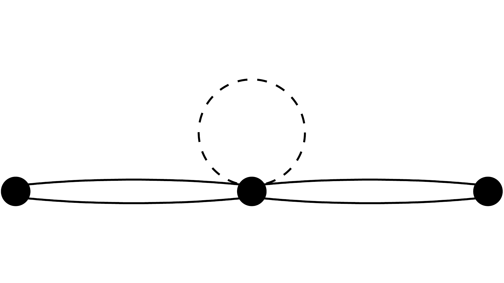
Figure 1. The diagram of the Painlevé three equation.

The dashed line indicates that the loop has negative multiplicity. The corresponding Cartan matrix is

(4) $$C=\left(\begin{matrix}2&-2&0\\ -2&4&-2\\ 0&-2&2\end{matrix}\right).$$

The corresponding additive moduli space $\mathcal{M}^{*}$ for Painlevé three (from the standard Lax pair) is known to be the affine $D_{2}$ ALF space, and so it is natural to view this graph as the Dynkin diagram of type $\mathchoice{\accentset{\displaystyle\text{\smash{\raisebox{-5.59721pt}{$\widehatsym$}}}}{D}}{\accentset{\textstyle\text{\smash{\raisebox{-5.59721pt}{$\widehatsym$}}}}{D}}{\accentset{\scriptstyle\text{\smash{\raisebox{-3.91806pt}{$\widehatsym$}}}}{D}}{\accentset{\scriptscriptstyle\text{\smash{\raisebox{-2.7986pt}{$\widehatsym$}}}}{D}}_{2}$. As a further consistency check one can consider the intersection form from the corresponding De Rham moduli space (the Okamato space of initial conditions). It is known ([17] p.182) that the intersection form is the negative of $\mathchoice{\accentset{\displaystyle\text{\smash{\raisebox{-5.59721pt}{$\widehatsym$}}}}{A}}{\accentset{\textstyle\text{\smash{\raisebox{-5.59721pt}{$\widehatsym$}}}}{A}}{\accentset{\scriptstyle\text{\smash{\raisebox{-3.91806pt}{$\widehatsym$}}}}{A}}{\accentset{\scriptscriptstyle\text{\smash{\raisebox{-2.7986pt}{$\widehatsym$}}}}{A}}_{1}\oplus A_{1}$, i.e. $-\left(\begin{smallmatrix}2&-2&0\\ -2&2&0\\ 0&0&2\\ \end{smallmatrix}\right)$. This fits since one can choose another $\mathbb{Z}$-basis in which the intersection form is given by the negative of our $\mathchoice{\accentset{\displaystyle\text{\smash{\raisebox{-5.59721pt}{$\widehatsym$}}}}{D}}{\accentset{\textstyle\text{\smash{\raisebox{-5.59721pt}{$\widehatsym$}}}}{D}}{\accentset{\scriptstyle\text{\smash{\raisebox{-3.91806pt}{$\widehatsym$}}}}{D}}{\accentset{\scriptscriptstyle\text{\smash{\raisebox{-2.7986pt}{$\widehatsym$}}}}{D}}_{2}$ Cartan matrix (4):

Lemma 4.

The bilinear forms with matrices $\mathchoice{\accentset{\displaystyle\text{\smash{\raisebox{-5.59721pt}{$\widehatsym$}}}}{D}}{\accentset{\textstyle\text{\smash{\raisebox{-5.59721pt}{$\widehatsym$}}}}{D}}{\accentset{\scriptstyle\text{\smash{\raisebox{-3.91806pt}{$\widehatsym$}}}}{D}}{\accentset{\scriptscriptstyle\text{\smash{\raisebox{-2.7986pt}{$\widehatsym$}}}}{D}}_{2}$ and $\mathchoice{\accentset{\displaystyle\text{\smash{\raisebox{-5.59721pt}{$\widehatsym$}}}}{A}}{\accentset{\textstyle\text{\smash{\raisebox{-5.59721pt}{$\widehatsym$}}}}{A}}{\accentset{\scriptstyle\text{\smash{\raisebox{-3.91806pt}{$\widehatsym$}}}}{A}}{\accentset{\scriptscriptstyle\text{\smash{\raisebox{-2.7986pt}{$\widehatsym$}}}}{A}}_{1}\oplus A_{1}$ are equivalent over $\mathbb{Z}$.

Proof. $g^{T}\left(\begin{smallmatrix}2&-2&0\\ -2&2&0\\ 0&0&2\\ \end{smallmatrix}\right)g=\left(\begin{smallmatrix}2&-2&0\\ -2&4&-2\\ 0&-2&2\end{smallmatrix}\right)\qquad\text{where}\qquad g=\left(\begin{smallmatrix}0&1&0\\ 0&0&1\\ -1&1&0\\ \end{smallmatrix}\right).$ $\square$

This diagram should also be compared/contrasted with the “shape” for Painlevé 3 suggested in [11] Example 6.17 (and last shape in figure on p.928), and with that in the approach of [18].

The diagrams for Painlevé 4,5,6 have already been discussed in detail in [2, 3, 4, 5]. The diagrams for the six Painlevé equations are thus as follows:

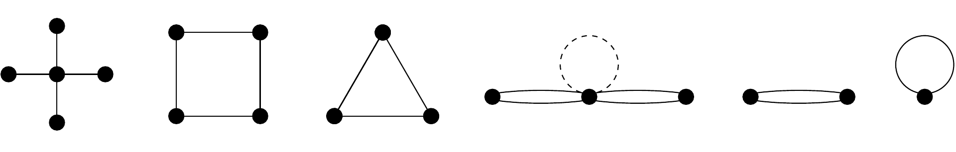
Figure 2. The diagrams of the six Painlevé equations.

Note that the number of nodes minus one is always the number of parameters in the corresponding Painlevé equation. Each node has dimension one, except for the central node in the Painlevé VI case, which has dimension $2$.

Remark 5.

Each of the Painlevé equations 2-6 has a special class of solutions coming from solutions of a linear differential equation ([16] p.310). We now understand the key statement: In each case the diagram of the linear equation is obtained by removing one node of the diagram for the corresponding Painlevé equation:

Painlevé equation	$P_{6}$ $\Bigl{|}$	$P_{5}$	$P_{4}$	$P_{3}$	$P_{2}$
Special solutions	Gauss ​​$\ {}_{2}F_{1}$$\Bigl{|}$	Kummer ​​$\ {}_{1}F_{1}$	Weber	Bessel–Clifford ​​$\ {}_{0}F_{1}$	Airy

Note that the discussion in [3, 4] implies the Kummer equation has diagram $A_{3}$ and the Gauss equation has diagram $D_{4}$. Also [16] just writes “Bessel” for the special solutions of $P_{3}$, but the Bessel equation $x^{2}y^{\prime\prime}+xy^{\prime}=(\nu^{2}-x^{2})y$ is really just a special one parameter subfamily of the Kummer (​​$\ {}_{1}F_{1}$) equations (up to a twist)—it is the subfamily that are pullbacks of a ​​$\ {}_{0}F_{1}$ equation (studied by Clifford): If $f$ satisfies $xf^{\prime\prime}+af^{\prime}=f$ then $x^{a-1}\cdot f(-x^{2}/4)$ satisfies the Bessel equation with parameter $\nu=a-1$, for example:

$$J_{\nu}(x)=\frac{(\frac{1}{2}x)^{\nu}}{\Gamma(\nu+1)}.\ _{0}F_{1}(\nu+1;-x^{2}/4).$$

Appendix A Sketch of proof of Prop. 3

Recall from [8] that the space $\mathcal{B}:=\operatorname{Hom}_{\mathbb{S}}(\Pi,G)$ is isomorphic to $\mathcal{A}/\!\!/G$, where $\mathcal{A}\cong G\times H(\partial)\times\operatorname{{\mathbb{S}}to}$ is the fission space, $H(\partial)$ is a twist of $H$ and $\operatorname{{\mathbb{S}}to}$ is the product of the Stokes groups (which has dimension $\text{\rm Irr}\operatorname{End}(\Theta)$). [8] shows that $\mathcal{A}$ is a twisted quasi-Hamiltonian $G\times H$ space, with a moment map $\mu=(\mu_{G},\mu_{H})$ to $G\times H(\partial)$. The $G$ action is free which implies $\dim\mathcal{B}=\dim\mathcal{A}-2\dim G$. In turn $\mathcal{M}_{\text{\rm B}}({\bf\Sigma},\mathcal{C})=\mathcal{B}/\!\!/_{\widetilde{\mathcal{C}}}H=\mu_{H}^{-1}(\widetilde{\mathcal{C}})/H$ is the tq-Hamiltonian reduction (of the stable points) by $H$ at the twisted conjugacy class $\widetilde{\mathcal{C}}\subset H(\partial)$ determined by $\mathcal{C}$. This has dimension $\dim(\mathcal{B}\times\widetilde{\mathcal{C}})-2\dim(H)+2$, since $H/Z(G)$ acts effectively on stable points, and the result follows.

A better approach is to frame the corresponding Stokes local systems slightly differently, as follows (this won’t work for arbitrary reductive groups): Just choose one basepoint on each circle $\langle q_{i}\rangle$, and frame there. The resulting space of framed Stokes local systems has the form $\mathcal{E}:=\mathcal{B}/H^{\perp}$ where $H^{\perp}\cong\prod_{1}^{m}{\mathop{\rm GL}}_{n_{i}}(\mathbb{C})^{\beta_{i}-1}\subset H$ (forgetting most of the old framings). This has a residual action of $\check{H}:=\prod_{1}^{m}{\mathop{\rm GL}}_{n_{i}}(\mathbb{C})$ (changing the remaining framings), and one can deduce from [8] that $\mathcal{E}$ is a quasi-Hamiltonian $\check{H}$-space, with moment map given by the formal monodromy, all the way around each circle $\langle q_{i}\rangle$ (cf. [7] p.1—there is only one outer boundary circle). Then $\mathcal{M}_{\text{\rm B}}({\bf\Sigma},\mathcal{C})=\mathcal{E}/\!\!/_{\mathcal{C}}\check{H}$ is just the q-Hamiltonian reduction at the class $\mathcal{C}\subset\check{H}$. The space $\mathcal{E}$ behaves as if it were the space of invertible representations of the “doubled quiver” given by the core $\Gamma$—one can identify directly the positive terms in (1),(2) with generators (Stokes arrows [7], plus formal monodromies) and the negative terms with relations (from $\mu_{G}=1$). The dimension count is then standard, as in [5] §9.1.

Acknowledgments. The second named author was supported by JSPS KAKENHI Grant Number 18K03256.

Laboratoire de Mathématiques d’Orsay,
Univ. Paris-Sud, CNRS,
Université Paris-Saclay,
91405 Orsay, France

philip.boalch@math.u-psud.fr

Department of Mathematics,
Faculty of Science Division I,
Tokyo University of Science
1-3 Kagurazaka, Shinjuku-ku,
Tokyo 162-8601, Japan

yamakawa@rs.tus.ac.jp

References

• [1] P. P. Boalch, Symplectic manifolds and isomonodromic deformations, Adv. in Math. 163 (2001), 137–205.
• [2] by same author, Quivers and difference Painlevé equations, Groups and symmetries: From the Neolithic Scots to John McKay, CRM Proc. Lect. Notes, 47, 2009, arXiv:0706.2634, 2007.
• [3] by same author, Irregular connections and Kac–Moody root systems, $\mathrm{arXiv\!:\!0806.1050}$, 2008.
• [4] by same author, Simply-laced isomonodromy systems, Publ. Math. I.H.E.S. 116 (2012), no. 1, 1–68.
• [5] by same author, Global Weyl groups and a new theory of multiplicative quiver varieties, Geometry and Topology 19 (2015), 3467–3536.
• [6] by same author, Wild character varieties, meromorphic Hitchin systems and Dynkin diagrams, (2018), Geometry and Physics II: A Festschrift in honour of Nigel Hitchin, pp.425-446, arXiv:1703.10376.
• [7] by same author, Topology of the Stokes phenomenon $\mathrm{arXiv\!:\!1903.12612}$, 2019.
• [8] P. P. Boalch and D. Yamakawa, Twisted wild character varieties, arXiv:1512.08091.
• [9] A. S. Dancer, Dihedral singularities and gravitational instantons, J. Geom. Phys. 12 (1993), no. 2, 77–91.
• [10] R. Garnier, Sur des équations … et sur une classe d’équations nouvelles d’ordre supérieur dont l’intégrale générale a ses points critiques fixes, Ann. Sci. ÉNS (3) 29 (1912), 1–126.
• [11] K. Hiroe, Linear differential equations on the Riemann sphere and representations of quivers, Duke Math. J. 166 (2017), no. 5, 855–935.
• [12] K. Hiroe and D. Yamakawa, Moduli spaces of meromorphic connections and quiver varieties, Adv. Math. 266 (2014), 120–151, arXiv:1305.4092.
• [13] M. Jimbo and T. Miwa, Monodromy preserving deformations of linear differential equations with rational coefficients II, Physica 2D (1981), 407–448.
• [14] N. Joshi, A. V. Kitaev, and P. A. Treharne, On the linearization of the Painlevé III-VI equations and reductions of the three-wave resonant system, J. of Math. Phys. 48 (2007), 42.
• [15] B. Malgrange, Équations différentielles à coefficients polynomiaux, Progr. in Math., vol. 96, 1991.
• [16] K. Okamoto, The Painlevé equations and the Dynkin diagrams, Painlevé transcendents (Sainte-Adèle, PQ, 1990), NATO ASI Ser. B, vol. 278, Plenum, New York, 1992, pp. 299–313.
• [17] H. Sakai, Rational surfaces associated with affine root systems and geometry of the Painlevé equations, Comm. Math. Phys. 220 (2001), no. 1, 165–229.
• [18] D. Yamakawa, Quiver varieties with multiplicities, Weyl groups of non-symmetric Kac-Moody algebras, and Painlevé equations, SIGMA 6 (2010), Paper 087, 43.