remresetThe remreset package
Quivers for tilting modules
Abstract.
Using diagrammatic methods, we define a quiver with relations depending on a prime and show that the associated path algebra describes the category of tilting modules for in characteristic . Along the way we obtain a presentation for morphisms between -Jones–Wenzl projectors.
1. Introduction
Let denote an algebraically closed field and the additive, -linear category of (left-)tilting modules for the algebraic group . This category can be described as the full subcategory of -modules which is monoidally generated by the vector representation , and which is closed under taking finite direct sums and direct summands.
The purpose of this paper is to give a generators and relations presentation of by identifying it with the category of projective modules for the path algebra of an explicitly described quiver with relations. This quiver can be interpreted as the semi-infinite Ringel dual of in the sense of [BS18]. For of characteristic zero this is trivial as is semisimple, and the indecomposable tilting modules are indeed the simple modules. The quantum analog at a complex root of unity is related to the zigzag algebra with vertex set and a starting condition, see e.g. [AT17].
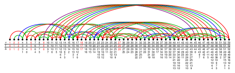
The focus of this paper is on the case of positive characteristic , for which we represent as a quotient of the path algebra of an infinite, fractal-like quiver, a truncation of which is illustrated for in Figure 1.
The main result
From now on let be an algebraically closed field of characteristic , and let be the corresponding special linear group. Recall that the indecomposable tilting modules for are classified (up to isomorphism) by their highest weight , and we pick a collection of representatives denoted by .
Theorem A
There is an algebra isomorphism
which sends the constant path on the vertex to the idempotent for the summand .
Let denote the category of finitely-generated, projective (right-)modules for . By semi-infinite Ringel duality [BS18, Section 4], we have the following consequence of A.
Corollary A
There is an equivalence of additive, -linear categories
sending indecomposable tilting modules to indecomposable projectives.
Several classical facts about -modules are reflected in the presentation of the algebra . For example, a path from to can only be non-zero in if and share a common Weyl factor. More specifically, if the -adic expansion has exactly non-zero digits, then has exactly Weyl factors where is obtained by negating some of the non-zero digits for . In this case, contains arrows from to those that are obtained by negating a single digit.
Our assignment of morphisms to arrows uses the Temperley–Lieb category. In contrast to other descriptions of morphisms between indecomposable tilting modules for , this presentation of is well-adapted to study as a monoidal category.
The Weyl factors in indecomposable tilting modules are illustrated in the lines , , in Figure 1, where the colors distinguish arrows in different blocks, the connected components of the quiver, and each reddish number corresponds to the unique simple tilting module in its block.
The algebra in a nutshell
We define the algebra as a quotient of the path algebra of an infinite, fractal-like quiver over the prime field . (In particular, we can always extend the algebra to an algebra over .) We will use this introduction to sketch the main features of and relegate the precise statement to Theorem 3.1.
-
The underlying quiver. We identify the vertex set with and the constant path at the vertex will be denoted (it corresponds to ). If , then for every digit with there is a pair of arrows
where .
-
Some relations. Up to some additional rules in special cases (which we ignore for the sake of this introduction), there are five types of relations among paths, which hold whenever both sides are defined and satisfy certain admissibility conditions.
-
(1)
Idempotents. , and , where is a word in the generators starting at and ending at . (Throughout, we use such relations to absorb all but one idempotent in each string of generators.)
-
(2)
Nilpotency. .
-
(3)
Far-commutativity. , , as well as whenever .
-
(4)
Adjacency relations. and , and scaled versions and .
-
(5)
Zigzag. .
Here , , and are scalars that depend on and the digit .
-
(1)
-
Hom spaces. For the -vector space is spanned by paths of the form with , i.e. paths that descend before ascending again. In particular, we have whenever for , which reflects the fact that the corresponding tilting module is simple.
-
Endomorphism algebras. Let have non-zero digits with indices . Then we have the following identifications of -algebras
This leads to a description of the endomorphism algebra of which could have been expected from Donkin’s tensor product theorem [Don93, Proposition 2.1].
We would like to highlight that we will meet a law of small primes (losp) repeatedly. By this we mean the appearance of exceptional relations in cases of -adic expansions with digits , , , or . These relations are exceptional in the sense that they contrast with the relations shown above, which describe the behavior of generic -adic expansions for large primes . Nevertheless, exceptional relations are relevant for all primes, and for only exceptional relations apply.
A word about the proof of A
The basis for our work is the classical fact that the Temperley–Lieb algebra controls the finite-dimensional representation theory of . The second main ingredient is an explicit description of -Jones–Wenzl projectors [BLS19], which are characteristic analogs of the classical Jones–Wenzl projectors, that diagrammatically encode the projections
The bulk of this paper is devoted to a careful study of morphisms between -Jones–Wenzl projectors over and the linear relations between them. This work was supported by extensive computer experimentation using Mathematica and SageMATH.
Relations to other work
To the best of our knowledge, the quiver underlying the tilting category is new: We study as a finitely presented category. So our main concern are the relations among composites of generating morphisms, rather than just the combinatorics of objects or the dimensions of morphism spaces, which appear in the classical literature.
We would like to acknowledge and reinforce that the representation theory is, of course, well-understood on the level of the modules, see e.g. [CC76], [AJL83], [Don93], [EH02a], [EH02b] and [DH05]. Further, various other quivers associated to are known, describing e.g. rational modules [MT11] or the extension algebra for simple [MT15] or Weyl modules [MT13].
A graded extension and translation functors
It is possible to give a similar quiver description of as a positively graded module category of the diagrammatic Soergel category for the Weyl group of type , acting by translation functors. The first step in such an extension uses the quantum Satake equivalence (at ) [Eli17] to connect the Temperley–Lieb diagrammatic calculus to . In fact, faithfully describes the degree zero part of the antispherical module category for . The second step uses ideas from [RW18] to relate and the principal block as long as . Along this route, also inherits a grading from .
In this case, the algebra essentially describes the degree zero part of the principal block , while the positive degree part is generated by additional degree arrows and , which interact non-trivially with other paths. Note another fractal-like structure: describes , but also the degree zero part of . We will not pursue this extension in the present paper.
Characteristic zero and higher rank cases
Throughout we could allow the case of characteristic zero, for which is semisimple. In a more interesting variant, one replaces by its quantum group analog at a complex root of unity, using the Jones–Wenzl projectors from [GW93]. The role of is then played by the zigzag algebra with vertex set and a starting condition, and we would recover a result of [AT17]. In this sense we think of as a positive characteristic version of the zigzag algebra.
We also like to highlight that, to the best of our knowledge, a quiver underlying tilting modules for higher rank groups is still unknown, even for the quantum group analog in characteristic zero, cf. [MMMT20, Section 5C] for some first steps in this direction.
We expect the diagrammatic methods used in this paper to generalize to and . This would involve developing characteristic analogs of so-called clasps, living in the corresponding web calculus, see e.g. [CKM14] or [TVW17], defined over .
Acknowledgments. D.T. likes to thank Henning Haahr Andersen, Ben Elias, Hankyung Ko, Catharina Stroppel and Geordie Williamson for teaching him everything he knows about tilting modules (which is basically nothing, but that is his fault alone). P.W. would like to thank James Borger, Ben Elias, Alexandra Grant, Anthony Licata and Scott Morrison for useful discussions. Special thanks to Henning Haahr Andersen, Jieru Zhu and an anonymous referee for valuable comments on a draft of this paper, to Nicolas Libedinsky for sharing a draft of the lovely paper [BLS19], which started this project, and Noah Snyder for pointing out a missing argument in the proof of Proposition 2.8.
Parts of this research were conducted while D.T. visited the Australian National University, supported by the Mathematical Sciences Research Visitor Program (MSRVP), and while P.W. visited Universität Zürich. Their hospitality and support are gratefully acknowledged. P.W. was supported by Australian Research Council grants ‘Braid groups and higher representation theory’ DP140103821 and ‘Low dimensional categories’ DP160103479
2. The Temperley–Lieb calculus
Let be a pivotal category with (strict) monoidal composition , unit , and duality . We usually write for the composition of morphisms. We read string diagrams for morphisms in from bottom to top and left to right, e.g.
The duality maps are pictured as cup and cap string diagrams, subject to the expected string-straightening relations. The pivotal structure additionally allows the rotation of string diagrams and guarantees that planar-isotopic diagrams represent the same morphism.
Let be any commutative and unital ring. (For us will usually be or , the prime field of . However, it also makes sense to formulate everything for and .)
The category (see e.g. [KL94]) can be described as the pivotal -linear category with objects indexed by , and with morphisms from to being -linear combinations of unoriented string diagrams drawn in a horizontal strip between marked points on the lower boundary and marked points on the upper boundary , considered up to planar isotopy relative to the boundary and the relation that a circle evaluates to . The composition and tensor product operations are as described above.
Particular cases of the isotopy and circle relations are
In the following we will use labeled strands as shorthand notation for bundles of parallel strands:
We even omit these numbers or the lines altogether if no confusion can arise.
The category furthermore admits a contravariant, -linear involution which reflects string diagrams in a horizontal line. Several arguments in the following will use this up-down symmetry. However, we will usually not have a left-right symmetry.
Recall that is a free -module with a basis given by crossingless matchings. The through-degree of is the number of strands connecting the bottom to the top. More generally, the through-degree of a general morphism is defined via . Note that , and thus, form a sequence of nested (-)ideals in .
Instead of , the number of strands, let us now use , which will be crucial number for everything that follows.
Definition 2.0
For the JW projectors are the morphisms, which are recursively defined by
| (2-1) |
where we use a box with bottom and top strands to indicate .
Lemma 2.1
(See e.g. [KL94, Section
3].) We have
and . Furthermore, the following
properties hold, which are best expressed diagrammatically.
(2-2)
(2-3)
(2-4)
2A. Characteristic notions
As already suggested by the recursion (2-1), the JW projectors have rational coefficients with respect to and typically cannot be defined in . To formalize this, consider the -adic valuation , defined for as (including ) and for as .
Definition 2.1
For a non-zero we let . We call such a morphism -admissible if .
To highlight morphisms that might not be -admissible, we use as e.g. in (2-1). Note that is -admissible if and only if every coefficient can be presented as a reduced fraction with . In this case, represents an element of , which is zero if and only if . If we write with and , then .
Example 2.1
We have for , which corresponds to the fact that the characteristic zero Weyl module stays simple when reduced modulo . However, for , one typically has , and in such cases the projectors cannot be defined in .
However, there are alternative idempotents satisfying and we will consider their specializations . To this end, recall that we write for the -adic expansion of with digits and . (More generally, we also write for any .)
Definition 2.1
If has only a single non-zero digit, then is called an eve. The set of eves is denoted by . If , then the mother of is obtained by setting the rightmost non-zero digit of to zero. We will also consider the set of (matrilineal) ancestors of , whose size is called the generation of .
Note that if and only if , and for we write for its eve.
Definition 2.1
For , the support is the set of the integers of the form . The integers for form the fundamental support of .
Example 2.1
Let . Then has , and and . Hence, the ancestry chart of is
Moreover, and . In pictures,
| (2-5) |
where we have highlighted in yellow the support of . The solid green arcs indicate successive inclusions in fundamental supports, and dashed orange arcs indicate successive inclusions in non-fundamental supports, all starting from .
To account for losp we need the following admissibility conditions.
Definition 2.1
Let be a finite set. We consider partitions of into subsets of consecutive integers, which we call stretches (in the -adic expansion of ). For the purpose of this definition, we fix the coarsest such partition.
The set is called down-admissible for if:
-
(d1)
for every , and
-
(d2)
if and , then .
If is down-admissible for , then we define
Conversely, is up-admissible for if the following conditions are satisfied:
-
(u1)
for every , and
-
(u2)
if and , then .
If is up-admissible for , then we define
where we extend the digits of by for if necessary.
If is up-admissible, then we denote by the down-admissible hull of , the smallest down-admissible set containing , if it exists.
Example 2.1
Let . The set (here and in the following, we use vertical bars to highlight the coarsest partition into stretches) is down-admissible but not up-admissible for . On the other hand, is up-admissible, but not down-admissible for , and we get
Here we have underlined the stretches of digits in and . Furthermore, .
Example 2.1
We think of the operations and as reflecting down and up along , respectively. The admissibility restrictions ensure that the down-admissible sets are in bijection with the elements and that reflecting down and up are inverse operations as we will see in Lemma 2.3. Explicitly, for and one gets
See also (2-5).
Definition 2.1
For two non-empty sets we define
We say and are distant if , adjacent if , or overlapping if .
If and are down- or up-admissible for and , then will also be down- or up-admissible, respectively. Conversely, if is down- or up-admissible for and , then need not be down- or up-admissible for .
For down- or up-admissible sets , a central object in the following will be the finest partition into down- or up-admissible subsets (the number is the size of this partition), which we order by size of their elements . Note that the elements of are necessarily consecutive integers, and that this partition is typically finer than the partition considered in Section 2A. We call the minimal down- or up-admissible stretches of , respectively. It is easy to check that
for down- or up-admissible , respectively.
Example 2.1
For the set (partitioned into stretches by the bar) and as in Section 2A the finest down-admissible partition is where . More generally, the down-admissible sets with are exactly the minimal down-admissible stretches for .
If is also down- or up-admissible and distant from , i.e. , then we have:
| (2-6) |
If and are subsets of , we write to indicate the requirement that every element in be strictly greater than every element in . We have the following equivalences of admissibilities.
Lemma 2.2
Consider stretches with .
-
(a)
is down-admissible for and is down-admissible for if and only if is down-admissible for and is up-admissible for . In this case we have .
-
(b)
is up-admissible for and is up-admissible for if and only if is down-admissible for and is up-admissible for . In this case we have .
Proof.
We prove (a). For this we write , and .
is down-admissible for if and only if and , and we get
Now is down-admissible for if and only if and , and we get
Conversely, is down-admissible for if and only if and , and we get
Now is up-admissible for if and only if and . This shows the equivalence of admissibilities. Furthermore, by reflecting up along , it is easy to see . The case of (b) is analogous. ∎
Lemma 2.3
Let and finite.
-
(a)
If is up-admissible for , then is down-admissible for and .
-
(b)
If is down-admissible for , then is up-admissible for and .
2B. Bookkeeping for caps and cups
For this section, we fix .
Definition 2.3
For we consider and to define (down and up) diagrams in via
This includes the case of , for which we have . Note that we use symbols such as to indicate the source or target of these morphisms.
Now, suppose that and are down-, respectively, up-admissible for . Then we set
| (2-9) |
In (2-9) and in the following we use the usual notation of idempotented algebras to drop some of the involved idempotents. Further, the different orderings of the factors in and ensure that stretches of consecutive integers in and give rise to nested caps and cups, respectively.
Lemma 2.4
For with the following hold.
-
(a)
is down-admissible for and is down-admissible for if and only if and are down-admissible for . In this case we have .
-
(b)
is up-admissible for and is up-admissible for if and only if and are up-admissible for . In this case we have .
-
(c)
If is up-admissible for and is down-admissible for , then is up-admissible for . In this case we have .
-
(d)
If is up-admissible for and is down-admissible for , then is down-admissible for . In this case we have .
Proof.
The claims about admissibility are not hard to prove and follow, mutatis mutandis, as in the proof of Lemma 2.2 given above. Finally, the equalities as e.g. are isotopies. ∎
Definition 2.4
Using the same notation as in Section 2B, we define diagrams in
The boxes represent JW projectors of the size implicit in the diagram, namely .
Definition 2.4
Suppose that is down-admissible for and is up-admissible for . Then we define trapezes and standard loops
Note that the diagrams defined in Section 2B are not left-right symmetric.
Example 2.4
For we have:
We record that , , and .
2C. The -Jones–Wenzl projectors
For and let denote the youngest ancestor of whose th digit is zero. (By convention, .) For each down-admissible for we let
| (2-10) |
Note that .
Example 2.4
Let and . Then we have , so the overall sign is positive. The relevant reflected ancestors in the telescoping product (2-10) are , , , and . So we get
The following is immediate from (2-10).
Lemma 2.5
If are down-admissible for , then .
As we will see below, the following definition is a reformulation of [BLS19, Section 2.3].
Definition 2.5
For the rational JW projector is defined to be
| (2-11) |
Example 2.5
For we have
Lemma 2.6
The elements agree with the ones defined in [BLS19, Section 2.3]. (Note however that we have mirrored their definition.)
Proof.
Careful inspection of the recursive definition in [BLS19, Section 2.3]. More precisely, in our notation their recursion works as follows. If , then . Otherwise,
| (2-12) |
where is the first non-zero digit of . ∎
Proposition 2.7
([BLS19, Theorem 2.6].) For any we have .
Definition 2.7
We define the JW projectors .
In illustrations we distinguish the three types of JW projectors via
called JW, rational JW and JW projectors, respectively.
Example 2.7
Note that these projectors behave quite differently, e.g. for the projectors as in Section 2C we have
Proposition 2.8
We have a pivotal, -linear functor
which sends the idempotent to the projection . This functor induces an equivalence of pivotal -linear categories upon additive Karoubi completion.
Proof.
By 2.7 and the construction of , the only non-trivial statement is the fully-faithfulness of . This is known; however, for completeness, let us give a short (but not new, cf. [Eli15, Theorem 2.58] or [AST17, Proposition 2.3]) argument for this. First, the same statement over is a classical result and dates back to work of Rumer–Teller–Weyl. This implies that hom spaces on both sides have the same dimension over . The point is now the flatness of both sides. Precisely, the standard basis works for , showing that the dimensions of hom spaces in are independent of the characteristic. The same is true in the image of : The module is a tilting module regardless of the characteristic, and the same thus holds for . This implies that the hom spaces in are also independent of the characteristic. Finally, one can check that remains linear independent, and the claim follows since all involved dimensions are finite and the same on both sides. ∎
3. The quiver algebra
3A. Generators and relations
In order to prove A we have to give a presentation of the algebra
| (3-1) |
by generators and relations. To this end, we first introduce notation for certain elements.
Definition 3.0
Let and be down- and up-admissible for , respectively. Then we define
| (3-2) |
We call the latter the loop on down through .
We will consider the morphisms and as generators for , but restrict to the cases when and are minimal admissible stretches of consecutive integers. Then these morphisms can be pictured as
We define two functions (where we again see losp) via
Note that and for . Then for each finite we define scaling operators on as
These are not considered as generators of , but as mere bookkeeping devices for the appearing scalars.
Theorem 3.1
(Generators and relations.) The algebra is generated by for , and elements and , where and denote minimal down- and up-admissible stretches for , respectively. These generators are subject to the following complete set of relations.
-
(1)
Idempotents.
-
(2)
Containment. If , then we have
-
(3)
Far-commutativity. If , then
-
(4)
Adjacency relations. If and , then
-
(5)
Overlap relations. If with and , then we have
-
(6)
Zigzag.
Here, if the down-admissible hull , or the smallest minimal down-admissible stretch with does not exist, then the involved symbols are zero by definition.
(Basis) The elements of the form
with , and , form a basis for .
(Complete) Any word in the generators of can be rewritten as a linear combination of basis elements from (Basis) using only the relations (1)–(6).
Remark 3.1
The algebra is a path algebra of an underlying quiver as follows. The idempotents correspond to vertices of a quiver, call these . The elements and correspond to arrows starting at the vertex , and either pointing to downwards or upwards (which is leftwards respectively rightwards in Figure 1) to or .
Remark 3.1
In the special case of , Theorem 3.1.(Basis) says that loops form a basis of the endomorphism spaces. Furthermore, we will see in Lemma 3.18 that all loops are products of loops for minimal down-admissible.
Remark 3.1
In Theorem 3.1.(4) and (6), the right-hand sides of the shown relations feature morphisms indexed by admissible subsets that are not necessarily minimal. We shall see in 3.10 that such morphisms decompose into products of generators
| (3-3) |
where the products are taken over the minimal down- respectively up-admissible stretches and , such that and , with and .
In Theorem 3.1 we use (3-3) as a shorthand notation, but one could also take and for (not necessarily minimal) admissible and as generators for . This requires listing the additional relations
| (3-4) |
for down-admissible with and up-admissible with , in addition to the relations Theorem 3.1.(1-6) among minimal generators. One advantage of such a presentation is that it exhibits as a quadratic algebra, since relations Theorem 3.1.(4-6) now turn into quadratic relations with respect to the enlarged generating set.
The proof of Theorem 3.1 will occupy the remainder of this paper. However, we already note that Theorem 3.1.(1) holds by the definition of as the endomorphism algebra of a direct sum. Moreover, assuming the relations Theorem 3.1.(1-6), we get:
Lemma 3.2
(Completeness—Theorem 3.1.(Complete).) Let . Then there is a finite sequence of relations Theorem 3.1.(1-6) rewriting it as a linear combination of elements of the form Theorem 3.1.(Basis).
Proof.
We can immediately restrict to the case where is a product of generators of (rather than a linear combination of such). In order to prove the claim, we will show that, if is not of the desired form, then we can measure its complexity by counting out-of-order pairs of the following forms, all other pairs are called in-order.
-
(i)
or for .
-
(ii)
.
A case-by-case check will verify that we can use our relations to reduce these to in-order pairs, which then inductively shows the claim. For the case-by-case check we write down the list of all combinations how stretches and can meet. A priori, there are such cases illustrated by
where the solid line represents and the dashed line , with smaller entries appearing further to the right. Some of the illustrated cases never arise when considering minimal admissible stretches and the remaining cases are precisely covered by our relations. Let us do this in detail for the out-of-order pair . First, the cases 2a)–2e) as well as 1e) and 3c) are ruled out by the assumption . The case 1a) is far-commutativity, the case 1b) adjacency, while 1d) and 3b) are covered by containment. The relation 3a) does not occur as would not be minimal. The remaining case 1c) is only possible if , in which case we can apply the overlap relation. ∎
3B. Basic properties of JW projectors
We invite the reader to illustrate the statements and proofs of the next lemmas using the explicit diagrammatic examples of trapezes from Section 2B and of JW projectors from Section 2C.
Lemma 3.3
Lemma 3.4
Suppose is down-admissible for , and is a minimal down-admissible stretch for . Then we have
We will also use the non-zero cases in the form:
| (3-5) |
Proof.
Lemma 3.5
Suppose that is the smallest minimal down-admissible stretch for and let be down-admissible for . Then we have:
| (3-6) |
Proof.
Similar, but easier than the proof of Lemma 3.4. ∎
Lemma 3.6
Let and . Then we have
Proof.
The first pair of equalities is clear since contains with coefficient and otherwise only cap and cup diagrams, which are killed by (2-3). For a down-admissible set , let . For the second pair of equalities we express as
It follows from 3.3 that the summands are orthogonal idempotents. Note that we can write for some morphism . In particular absorbs or smaller, and it annihilates all for . In particular, it absorbs . ∎
Proposition 3.7
(Classical absorbtion.) Let . Then we have
Proof.
We distinguish two cases. If , then we have
and the other equation follows by reflection.
On the other hand, if , then . Let denote the youngest common ancestor of and . It follows that is the oldest ancestor of with . Now, we have and for any , as well as
The latter is a consequence of 3.3. Moreover, for each , there exists exactly one , such that . Thus, we have
The computation for is analogous. ∎
Example 3.7
For we have
We also have the following relations with no classical analog.
Proposition 3.8
(Non-classical absorbtion and shortening.) Let be a down-admissible stretch for . Then we have
Here denotes the youngest ancestor of for which the th digit is zero.
Proof.
If suffices to prove these relations in the case of minimal down-admissible stretches. To be consistent with the above notation, let us write instead of .
In order to verify the first relation we compute, using (3-5), that
| (3-7) |
For with , we define . For with , we define . It is easy to verify that the sets and are down-admissible for .
Then 3.3 implies that each summand in (3-7) is invariant under left multiplication by a unique summand in , while it is killed under left multiplication by any other summand. This proves the first equation; the second absorption equation follows by reflection symmetry.
For later use, note that the relevant summands of are the for which or .
Now we are ready to prove the projector shortening relations. We start by expanding
Note that the down-admissible sets for are exactly the down-admissible sets of which are contained in and that . Recall that, by (3-6), we have
| (3-8) |
In the resulting elements we either see , with or with .
Now, if is down-admissible for , we compute
where the scalars and are computed as follows.
Thus, by (3-8), we have
This establishes the third relation. The analogous relation for cups follow by reflection. ∎
The characteristic analog of (2-4) is:
Proposition 3.9
(Partial trace.)
-
(a)
For , being the first non-zero digit of , we have
(3-9) On the other hand, if and , then the (partial) trace of is zero.
-
(b)
Let be down-admissible for and the smallest minimal down-admissible stretch for . Then the partial trace on the bundle of strands specified by evaluates as:
Proof.
The second claim in Proposition 3.9.(a), concerning the case of , follows from and (2-4), which produces a scalar with . The case follows immediately by applying (2-4) to the two expressions in the bracket in (2-12).
In Proposition 3.9.(a) we have already seen the case , so we assume that . We then apply the projector shortening relations from Proposition 3.8, and get the following two cases for , depending on whether or .
Here we have used Proposition 3.9 for the second equation in the bottom row. ∎
3C. Morphisms between JW projectors—the linear structure
First, we state direct consequences of classical absorption, see Proposition 3.7, and non-classical absorption, see Proposition 3.8.
Lemma 3.10
-
(a)
If with , each down-admissible for , and with , each up-admissible for , then
-
(b)
Let and be down- and up-admissible for , respectively. Then we have
Here denotes the youngest ancestor of for which all digits with indices in are zero.
Let be a cap (or cup) configuration, i.e. a Temperley–Lieb diagram consisting only of caps (or cups), with source (target) . We say that is ancestor-centered for , and write , if each cap or cup has its center immediately to the right of an ancestor strand of .
Example 3.10
A way to illustrate ancestor-centering is imagine a line with a marker to the right of each ancestor strand of . (There are strands in total and many .) For example, for and we have
Moreover, we have , with mid point right to . More generally, the morphisms and are ancestor-centered if is down- or up-admissible, respectively.
The following is the analog of (2-3).
Lemma 3.11
For a cap configuration we have unless . Analogously for cup configurations.
Proof.
Lemma 3.12
-
(a)
Suppose that and are down-admissible for and , respectively, with . Then we have
(3-10) for some coefficients , where and are down-admissible for and , respectively, and . (In other words .)
-
(b)
We have isomorphisms of -vector spaces
(3-11) where ranges over pairs of sets that are down-admissible for and , respectively, such that . In particular, .
Note that the second isomorphism in (3-11) is unitriangular by (3-10). We will refer to morphisms of the form as standard morphisms and to morphisms of the form as -morphisms.
Proof.
The proof of (a) proceeds by iterating Lemma 3.4. Let and be the partitions into minimal admissible stretches of consecutive integers with the usual ordering. Then we expand
since by (3-5), we have if , and otherwise and thus . Here we write for the ideal of morphisms of smaller through-degree than the leading term. We now iterate this argument to find
which together imply (3-10).
Lemma 3.13
(Theorem 3.1.(Basis).)
-
(a)
Suppose that a -admissible morphism is expressed as
(3-12) where and the sum ranges over pairwise distinct pairs of sets that are down-admissible for and , respectively, such that . Then every coefficient is -admissible.
-
(b)
We have the -vector space isomorphisms
where ranges over the same set as above. In particular
Proof.
For the first claim, we proceed by induction on the through-degree. Note that the through-degree of is . Let be the pair labeling the summand with maximal through-degree. Then is -admissible since it is the coefficient of the (maximal through-degree) basis element in (3-12). Thus, we can subtract to obtain another -admissible sum, which now has strictly lower through-degree since was the only summand with this maximal through-degree. If the resulting sum is non-zero, then the remaining coefficients are now -admissible by the induction hypothesis. The basis step for the induction concerns the morphism of minimal possible through-degree, which is -admissible (and thus also its coefficient) since there are no correction terms in (3-10).
To see (b), for any given , we choose a lift . By (3-11), the -admissible morphism can be expanded in the -morphism basis over . By (a), all appearing coefficients are -admissible and can be specialized to . This results in an expansion of in terms of the -morphisms over . Note that all such morphisms are still linearly independent, since they have distinct through-degrees. ∎
3D. Morphisms between JW projectors—the algebra structure
Lemma 3.14
-
(a)
The algebra is commutative.
-
(b)
Every is nilpotent. As a consequence, every element of non-maximal through-degree in is nilpotent.
Proof.
By Lemma 3.13.(b), has a basis that is invariant under reflection. Thus, for all we have and , and then . This implies that is commutative.
To see (b), we shall use induction on . We work over and start by expanding into a sum of orthogonal quasi-idempotents and noting that has eigenvalue divisible by . If was maximal, then we have in . Otherwise, if , we conclude . By Lemma 3.13.(b), is a linear combination of loops with . Then the induction hypothesis implies that , and thus also , is nilpotent. ∎
Lemma 3.15
(Containment—Theorem 3.1.(2).) Let be a stretch that is down- or up-admissible for and down-admissible for or up-admissible for respectively. Then we have
Proof.
Note that by projector absorption, we have . This is a cap configuration consisting of a pair of collections of concentric caps. The right one is not ancestor-centered and, thus, kills by Lemma 3.11. ∎
Lemma 3.16
(Far-commutativity—Theorem 3.1.(3).) Suppose that and are down-admissible, and up-admissible and , , and . The following hold.
Proof.
These relations follow from projector absorption. For example, for the first relation we compute
Here we have used an isotopy of caps in the third equality. ∎
Lemma 3.17
(Adjacency relations —Theorem 3.1.(4).) If and , then the following equations hold whenever one side, and thus also the other one, is admissible
Proof.
The first relation follows from projector shortening and absorption, as can be best verified graphically, i.e.
Here we have used projector shortening twice, then projector absorption and an isotopy. The second relation is analogous. ∎
The following four statements will be proved jointly by induction in . The proofs depend on each other in a non-trivial way.
Lemma 3.18
(The endomorphisms.) Let with minimal down-admissible stretches . Then we have the algebra isomorphism
and if is down-admissible for , then . Furthermore, if is down-admissible for , then we have
| (3-13) |
Lemma 3.19
(Adjacency relations —Theorem 3.1.(4).) Let be down-admissible stretches of consecutive integers for with . Then we have
Lemma 3.20
(Overlap relations—Theorem 3.1.(5).) Suppose that is a minimal down-admissible stretch for and a minimal down-admissible stretch for with and , then we have
Lemma 3.21
(Zigzag—Theorem 3.1.(6).) Suppose that is an up-admissible stretch for . If is also down-admissible for , then we have
Here denotes the smallest minimal down-admissible stretch with , provided it exists. If not, then the equation holds without the second term on the right-hand side.
Furthermore, if is not down-admissible for , then we have
Here denotes the down-admissible hull of , if it exists. If not, then the right-hand side is defined to be zero.
4. Inductive proof of the relations
In this section we will use the far-commutativity relations from Lemma 3.16, the containment relations from Lemma 3.15, and the adjacency relations from Lemma 3.17, sometimes without explicitly mentioning them. Further, we only prove Lemma 3.19 and 3.20, and (3-13) for the first shown relations as the other ones are equivalent by reflection.
Convention 4.0
Throughout this section, unless stated otherwise, we use the convention that denotes either a minimal down- or up-admissible stretch for , and are the following minimal down-admissible stretches for . To declutter the notation, we will suppress symbols in many expressions, for example . Further, we introduce shorthand notation for the states where we have already proven the above Lemmas for certain .
-
means Lemma 3.21 holds for all zigzags of the form where and is down-admissible for , except possibly for the case and , the smallest minimal down-admissible stretch for .
-
means Lemma 3.19 on adjacent generators holds for all .
-
means Lemma 3.20 on overlapping generators holds for all .
-
means Lemma 3.21, holds for all zigzags of the form where .
-
means Lemma 3.18, which describes , holds for all .
Here we would like to draw the readers attention to the fact that the relevant quantity for zigzags is not where they start, but how high they reach.
The inductive proof of these conditions will proceed in the order shown. As base cases we observe that , , and are all vacuously satisfied for . Then, assuming that these conditions all hold for , we will first deduce , then and , followed by , and finally .
Lemma 4.1
follows if we have .
Proof.
We need to show that we can resolve all zigzags of the form where denotes a down-admissible stretch for such that , the smallest minimal down-admissible stretch for . If , then this is possible using projector absorption and . In the remaining cases we write and employ the same trick, but for . If is down-admissible for , we get
Here denotes the smallest minimal down-admissible stretch for , if it exists. We have also underlined the locations where relations are applied. If is not down-admissible for , then we instead get
or zero, if (and thus ) does not exist. ∎
4A. Adjacency relations
Next we focus on establishing . These relations are irrelevant for , so we will assume in this subsection. For this we need an approximate result first.
Lemma 4.2
Suppose that are adjacent minimal down-admissible stretches for . Then we have
Here is the span of morphisms with exceeding .
Similarly, if the stretches are up-admissible for , then we have
where .
In either case, if is a largest down-admissible stretch for , or if no down-admissible stretch exists above , then the relations from Lemma 3.19 hold on the nose.
Proof.
Let us write for the scalar appearing in . (The functions , , and were defined in Section 3A.) We would like to identify
By projector absorption it suffices to do this in the case when is the smallest minimal down-admissible stretch of . We will start by computing the characteristic zero analogs of both sides.
Suppose that is down-admissible for , then by Lemma 3.4 we have
After another application of Lemma 3.4 we get
| (4-2) |
These possibilities for index the -morphism basis for from Lemma 3.13. The term of maximal through-degree arises for . Now, by the unitriangularity of the basis change between -morphisms and standard morphisms, we can read off the coefficient of in the -morphism expansion of as the coefficient of in (4-2). Writing and , we compute this coefficient as
| (4-3) |
From this, we immediately get , as desired.
To finish the proof, we also need to show that (the basis morphism of second highest through-degree in ) does not occur in the -morphism expansion of . Thanks to triangularity of the basis change, this can be verified by computing the coefficient of in the difference , and showing that it reduces to zero modulo .
To this end, we again use Lemma 3.4 to expand
| (4-5) |
Focusing on the case , we compute the crucial coefficient as
| (4-6) |
where we have used , and in the first line, and in the second line
Now we note that
and together with (4-3) we can continue
This is divisible by and, thus, is zero modulo . This completes the proof of the first claim of the lemma. The second one is analogous. ∎
Lemma 4.3
follows if we have , and .
The proof will be split into two parts. First we give a proof that works under a technical assumption, which is generically satisfied. In the second part, we treat the remaining cases.
Proof, with caveat..
By and projector absorption we may assume that is a smallest down-admissible stretch. At first, we will also assume that are minimal down-admissible stretches for and that is also down-admissible for . By Lemma 2.4, this implies that is up-admissible for and is down-admissible for .
We already know that the desired equation holds up to certain potential error terms, i.e.
| (4-7) |
where the summation runs over down-admissible subsets , and where we write for . We now multiply this equation with on the left and with on the right and rewrite it using and Lemma 3.17 into
| (4-8) |
This equation can be simplified using . In this proof attempt, we only consider the generic case where (and thus also ) is down-admissible for . So, using for the pair we get:
where and are computed from . Further, using for and as well as we compute
where and are as above, while . We also have
(Note that is invertible since .) Using these two computations and , the equation (4-8) transforms into
Since the -loops form a basis of and the scalars and are non-zero by admissibility and , we conclude and then . Thus all error terms in (4-7) vanish. This completes the proof in the case where and are minimal.
In the general case, we partition and into minimal down-admissible stretches and , respectively. Then we have
Here we have first used far-commutativity, then on the adjacent minimal stretches , and finally Lemma 3.17. Note also that far-commutes with . ∎
Proof of the remaining cases.
In the previous proof we made the assumption that , and thus also , is down-admissible for . Now suppose this is not the case. At first we can proceed in a very similar way as in the previous proof. Whenever we use zigzag relations, we have to replace by and set the -term to zero. Hence, we get
and the equation (4-8) transforms into
This implies that the coefficients and are unit multiples of each other for every . Next we will use a different strategy to show that , which thus implies and finishes the proof. The strategy is to multiply both sides of (4-7) by on the right, to equate the first two terms, to kill all terms with coefficients , and to preserve all terms with coefficients .
The first two terms are rewritten as
which are equal by virtue of since . We also note that the scalar that appears is exactly . After subtracting these terms from the multiple of (4-7), we are left with
| (4-9) |
We first claim that . To verify this, we distinguish between the two cases in which is distant or adjacent to . In the first case, we get
since thanks to as . In the second case, we get
since . This proves the claim.
Our second claim is that for every and that these morphisms are linearly independent. Again it matters whether is distant or adjacent to . In the first case we get
Here we have used for to proceed to the second line. (We use to indicate unit proportionality.) In the second case we compute
This time we have used , namely on the ancestor using projector absorption, to get to the second and the fourth line, and in the form of a zigzag relation for , noting that is down-admissible for , to get to the third line. The proportionality constants that appear in these steps are units and are linearly independent as varies.
Finally, the two claims and equation (4-9) imply that for every , and thus also , which finishes the proof of . ∎
4B. Overlap relations
Next, we focus on establishing . We again start with an approximate version.
Lemma 4.4
Suppose that are adjacent minimal down-admissible stretches for and is a minimal down-admissible stretch for with and , then we have
Here we use the notations and . In either case, if is a largest down-admissible stretch for then the relations from Lemma 3.20 hold on the nose.
Proof.
We will use the notation and , , and note . We will also consider the minimal down-admissible stretch for , if it exists. For the purpose of this proof it is useful to explicitly write down the relevant parts of the continued fraction expansions of , and other entities
Here we have highlighted the digit in position in red.
From this description, it is straightforward to see that is spanned by morphisms of the following four different types
where denotes a down-admissible subset for with , which may be empty. The basis elements of highest and second highest through-degree among the above are and , and all other basis elements are in the subspace .
Our task is to show that appears with coefficient and appears with coefficient if we expand in this basis. We again start with a computation in characteristic zero.
The coefficient of the maximal through-degree basis element in is equal to the coefficient shown for in (4-12). This is
This shows that appears with coefficient in . The term , however, does not seem to appear at all in (4-12). Since it is of second highest through-degree in , its coefficient is congruent to the coefficient of in the -morphism expansion of .
Using Lemma 3.4, it is straightforward to compute that equals up to terms of lower through-degree. Thus, we compute the coefficient of interest as
and this finishes the proof. ∎
Lemma 4.5
follows if we have , , , and .
Proof, with caveat..
As usual, and projector absorption allows us to restrict to the case when is the smallest minimal down-admissible stretch for . By Lemma 4.4 we then have
| (4-13) |
Here denotes another adjacent minimal down-admissible stretch for , if it exists, and ranges over down-admissible subsets for . Our task is to show that the scalars are all zero.
We start by multiplying both sides of (4-13) by on the right. After rearranging, we get
| (4-14) |
The next step is to apply the zigzag relations and for this we shall assume that we are in the generic case, where is down-admissible for (and thus ). This also implies that is down-admissible for , and using the zigzag relations provided by for we compute
Similarly we compute
| (4-15) |
where we write and , and we have used on the pair and smaller instances, as well as . Thus, we have equated the first two terms in (4-14). We also simplify the terms
where we have again used on the pair , then , and smaller instances of zigzag relations in the case when is adjacent to for the final step. To be explicit, the sequence of transformations is
The simplification of the term proceeds in complete analogy to (4-15) and we get
having again used only and .
Finally, after all these simplifications, (4-14) gives the following linear system
which, since , implies that all unwanted scalars are zero. ∎
Proof of the remaining cases.
Now suppose that is not down-admissible for , which happens exactly if in the notation from above. In this case we have for and for .
We proceed exactly as above, with the only differences being that no terms arise and . The linear system resulting from (4-14) is
(Note that if , we immediately see .) To see that all coefficients are zero, we multiply (4-13) by , expecting that this should allow us to equate the first two terms, kill the and terms, and not hurt the and terms. Let us check these assertions in turn.
For the first term we get
For the second term we compute
where the second step works as in (4-15) and requires and . This equates the first two terms.
Now we claim that the and terms are killed by the loop along
If is adjacent to , then both assertions follow from
If is distant from or empty, then we use far-commutativity to see substrings of the form by .
Now we claim that the and terms survive the multiplication by the loop along :
To see this, let us first observe . This is clear if is distant from , and it follows from and , otherwise. Using this observation, we compute
where the last step works as in (4-15) and requires and .
After these simplifications, we see that (4-13) multiplied by shows , which (for ) in turn implies . This completes the proof of . ∎
Let us also note the following consequence.
Lemma 4.6
Suppose that a minimal stretch is down-admissible for but not for , and suppose the down-admissible hull exists. Then implies
| (4-16) |
Proof.
Let and and . Then is down-admissible for and we use to compute
The other relation follows by reflection. ∎
4C. Zigzag relations
Lemma 4.7
The zigzag relations from Lemma 3.21 hold in generation .
Proof.
Suppose that is a down-admissible stretch for such that is of generation . Then, using the projector shortening property from Proposition 3.8, we get
This partial trace is not covered by Proposition 3.9, but since is of generation at most , it can be straightforwardly computed: One first expands into a linear combination of standard loops and computes their partial traces using (2-4). The result follows by changing back into the loop basis of and reducing the coefficients to .
The basis change from loops to standard loops for of generation with minimal down-admissible stretches is
The inverse basis change can be readily computed from this. The basis change in generation is easier and left as an exercise for the reader. ∎
Lemma 4.8
follows if we have , , and .
The proof again splits into two parts. First we give a proof that works under a technical assumption, which is generically satisfied. In the second part, we refine this proof to work in all cases.
Proof, with caveat..
We need to consider the zigzag where is the smallest minimal down-admissible stretch of . Let us also assume that we are in the generic case, where is also down-admissible for (and thus ), and we denote by the minimal down-admissible stretch for that is adjacent and .
By the unitriangularity of the basis change between the loops basis and the standard loops basis for and by the generation case in Lemma 4.7, we may assume that
| (4-17) |
with error terms with . Our job is to show that we have for all such . If we multiply (4-17) by , then implies and thus , where runs over all as above, for which . On the other hand, if we multiply (4-17) by , then we get
where now runs over all remaining such that . Then, by , we also get
This implies for such . The only coefficients that are left to be considered are the ones for which . Now we apply the partial trace to both sides of (4-17). For this we will use the notation and , and we get
This is because where , which differs from by increasing its first non-zero digit by one. The coefficient of on the right-hand side is computed as follows
After subtracting the multiples of from both sides, we conclude . ∎
Proof of the remaining cases.
Now suppose that is smallest minimal down-admissible stretch for , but not down-admissible for . Then (4-17) takes the form
We first multiply this by and deduce
from . Since by , we get unless . Then a partial trace argument as above shows that all remaining are also zero. ∎
Lemma 4.9
follows if we have , , , and .
Proof.
We first prove (3-13). By and projector absorption, we may assume that is a smallest minimal down-admissible stretch. Suppose first that is down-admissible for . Then we have
where we have used , and finally to deduce . Now, suppose that is not down-admissible for . Then we instead get
Here we have used and Lemma 3.15.
Next we need to prove that and . The first relation simply follows from (3-13), i.e.
Next, suppose we already know that for subsets that decompose into minimal stretches, and let us now consider where . The result is clear if and are distant, so we will assume that is adjacent to . By projector absorption and (3-13), we may further assume that is the smallest minimal down-admissible stretch for . Then we compute
The equation and Proposition 3.9 imply where . Equivalently, we can write . Suppose that , then would be a unit in , so we can write
However, the left-hand side has through-degree , while the right-hand side has through-degree at most , a contradiction. Thus, we have and , and consequently . ∎
This completes the proof of Theorem 3.1, which by Proposition 2.8, completes the proof of A.
Remark 4.9
In addition to the eve base cases for the induction we have explicitly seen certain relations in cases of low generation. For example, for of generation , the description of the endomorphism algebra can be deduced from the proof of Lemma 3.14 while the adjacency and overlap relations hold vacuously. For of generation , we have seen the adjacency relations in Lemma 4.2 and the overlap relations in Lemma 4.4. Finally, zigzag relations for loops based at of generation were treated in Lemma 4.7.
5. Some conclusions
5A. The fractal nature of
The quiver underlying is a graph with countably infinitely many connected components. In each connected component there is a unique vertex with , and we denote the vertex set of this component by .
Example 5.0
We have , cf. (2-5).
The decomposition of the quiver implies that the algebra decomposes as
Let denote the free monoid on the set . We represent the elements of by words for and the multiplication is given by
(Note that the empty word is the neutral element.) Elements of with differing numbers of leading zeros are considered as distinct, and so they should not be interpreted as -adic expansions of natural numbers. However, carries an action of defined by
The fractal nature, i.e. the self-similarity, of is now captured by the following proposition.
Proposition 5.1
The monoid acts on by algebra endomorphisms: For each , there is an algebra endomorphism acting on idempotents by
and on arrows by reindexation. Moreover, we have
Finally, if , then maps any isomorphically to . In this sense, is generated under the action of by the summands for .
Proof.
This is a direct consequence of Theorem 3.1. ∎
We also note that, since is the direct sum of many copies of for , the underlying quiver of is a fractal graph in the sense of Ille–Woodrow [IW19], albeit in the trivial sense that any countable graph without edges and more than one vertex can be considered as a fractal factor.
5B. A few words about tilting modules
Let us work over the ground field . First, recall the category of finite-dimensional modules for has simple , Weyl , dual Weyl and indecomposable tilting modules for , the latter being the indecomposable objects of , see e.g. [Wil17, Section 1] for a concise summary of the main definitions and properties regarding .
Let us now elaborate a bit further on the representation-theoretic implications of A. Almost all of these are, of course, well-understood. However, the reader might find it helpful to see how they can be derived from our results in the previous sections.
It is well-known that
whose direct summands are called blocks, which are equivalent as additive, -linear categories. From our discussion we immediately get the following.
Proposition 5.2
There is an equivalence of additive, -linear categories
sending indecomposable tilting modules to indecomposable projectives. Moreover, if and for . Finally, there is an isomorphism of algebras for all with equal non-zero digits.
Proof.
Directly from A and A, combined with Theorem 3.1 and the above. ∎
In fact for all , but such isomorphisms involve non-trivial rescalings in our presentation.
Another consequence we get are the tilting–dual Weyl multiplicities.
Proposition 5.3
We have
Proof.
Note that the basis Theorem 3.1.(Basis) is part of the family of bases constructed in [AST18], and the proposition follows from the construction of these bases in loc. cit., and our main statements A and A. ∎
Hence, we get the tilting characters , where the characters are the characteristic zero characters well-known e.g. by Weyl’s character formula. By reciprocity, cf. [RW18, Proposition 1.14], we also get the Weyl–simple multiplicities. To state these explicitly, let us recursively define a set as follows. For let . For let
where we again meet losp. Then we get
Thus, we get , which determines the simple characters by inverting the change of basis matrix.
Example 5.3
For we have , cf. [JW17, Figure 1]. Moreover, we also get .
The final consequence we would like to derive in this paper is the following.
Proposition 5.4
Let . For any thick -ideal in there exists such that
with the latter equality holding in case .
Proof.
We will use that is a -generator of and Weyl and dual Weyl modules have classical characters.
Assume that for minimal. Then it is clear by Proposition 5.3 that . Thus, it remains to determine the possible minimal . To this end, note that the decomposition of into its indecomposable summands is completely determined by Proposition 5.3 and the classical tensor product combinatorics. Analyzing now how tensoring with affects the support, Proposition 5.3 then also implies that needs to be a prime power, and conversely, that a prime power works as a minimal .
Finally, the last statement follows from Proposition 3.9 since for . ∎
Thus, the thick -ideals in are .
Example 5.4
The elements of are the so-called negligible modules.
Note that the above implies that has no projective modules since these would form the minimal thick -ideal.
Table of notation and central concepts
In general we use a tilde, e.g. , to indicate that we work over , an overline, e.g. , to indicate that we have something that reduces mod but we want to consider it over , and no extra decoration if we work in .
| Name | Symbol | Description |
|---|---|---|
| Ringel dual of | the path algebra of a quiver with relations presented in Theorem 3.1. | |
| — | , , | functions used in the presentation of , Section 3A. |
| JW projector | the Jones–Wenzl projectors, corresponding to projections to in ; defined over , Section 2. | |
| JW projector | the Jones–Wenzl projectors, corresponding to projections to in ; defined over , Section 2C. | |
| rational JW proj. | the Jones–Wenzl projectors, corresponding to projections to in , but considered over , Section 2C. | |
| — | scalars in the definition of projectors (2-10). | |
| integral morphisms | down or up morphisms given by cups or caps; these work integrally, Section 2B. | |
| standard morphisms | down or up morphisms given by cups or caps together with JW projectors; these over , Section 2B. | |
| morphisms | down or up morphisms given by cups or caps together with JW projectors; these over , Section 3A. | |
| standard loops | compositions of down and up morphisms; form a basis of endomorphism spaces over , Section 2B. | |
| loops | compositions of down and up morphisms; form a basis of endomorphism spaces over , Section 3A. | |
| eve | a number with a single non-zero -adic digit, Section 2A. | |
| mother of | defined (unless is an eve) by setting the last non-zero -adic digit of to zero, Section 2A. | |
| ancestors of | positive numbers obtained by setting last -adic digits of to zero, Section 2A. | |
| generation of | the number of ancestors of , Section 2A. | |
| stretches | — | sets of consecutive digits in the -adic expansion of a number, Section 2A. |
| admissibility | — | whether a set of digits of a -adic expansion is suitable for reflecting up or down, Section 2A. |
| admissible hull | an admissible set containing , Section 2A. |
References
- [AJL83] H.H. Andersen, J. Jørgensen, and P. Landrock. The projective indecomposable modules of . Proc. Lond. Math. Soc. (3), 46(1):38–52, 1983. 10.1112/plms/s3-46.1.38.
- [AST18] H.H. Andersen, C. Stroppel, and D. Tubbenhauer. Cellular structures using -tilting modules. Pacific J. Math., 292(1):21–59, 2018. URL: https://arxiv.org/abs/1503.00224, doi:10.2140/pjm.2018.292.21.
- [AST17] H.H. Andersen, C. Stroppel, and D. Tubbenhauer. Semisimplicity of Hecke and (walled) Brauer algebras. J. Aust. Math. Soc., 103(1):1–44, 2017. URL: https://arxiv.org/abs/1507.07676, doi:10.1017/S1446788716000392.
- [AT17] H.H. Andersen and D. Tubbenhauer. Diagram categories for -tilting modules at roots of unity. Transform. Groups, 22(1):29–89, 2017. URL: https://arxiv.org/abs/1808.08022, doi:10.1007/s00031-016-9363-z.
- [BS18] J. Brundan and C. Stroppel. Semi-infinite highest weight categories. 2018. URL: https://arxiv.org/abs/1808.08022.
- [BLS19] G. Burrull, N. Libedinsky, and P. Sentinelli. p-Jones–Wenzl idempotents. Adv. Math., 352:246–264, 2019. URL: https://arxiv.org/abs/1902.00305, 10.1016/j.aim.2019.06.005.
- [CC76] R. Carter and E. Cline. The submodule structure of Weyl modules for groups of type . Proceedings of the Conference on Finite Groups (Univ. Utah, Park City, Utah, 1975). Pages 303–311, 1976.
- [CKM14] S. Cautis, J. Kamnitzer, and S. Morrison. Webs and quantum skew Howe duality. Math. Ann., 360(1-2):351–390, 2014. URL: https://arxiv.org/abs/1210.6437, doi:10.1007/s00208-013-0984-4.
- [Don93] S. Donkin. On tilting modules for algebraic groups. Math. Z., 212(1):39–60, 1993. doi:10.1007/BF02571640.
- [DH05] S. Doty and A. Henke. Decomposition of tensor products of modular irreducibles for . Q. J. Math., 56(2):189–207, 2005. URL: https://arxiv.org/abs/math/0205186, doi:10.1093/qmath/hah027.
- [Eli15] B. Elias. Light ladders and clasp conjectures. 2015. URL: https://arxiv.org/abs/1510.06840.
- [Eli17] B. Elias. Quantum Satake in type . Part I. J. Comb. Algebra, 1(1):63–125, 2017. URL: https://arxiv.org/abs/1403.5570, doi:10.4171/JCA/1-1-4.
- [EH02a] K. Erdmann and A. Henke. On Ringel duality for Schur algebras. Math. Proc. Cambridge Philos. Soc., 132(1):97–116, 2002. doi:10.1017/S0305004101005485.
- [EH02b] K. Erdmann and A. Henke. On Schur algebras, Ringel duality and symmetric groups. J. Pure Appl. Algebra, 169(2-3):175–199, 2002. doi:10.1016/S0022-4049(01)00071-8.
- [GW93] F.M. Goodman and H. Wenzl. The Temperley–Lieb algebra at roots of unity. Pacific J. Math., 161(2):307–334, 1993.
- [IW19] P. Ille and R. Woodrow. Fractal graphs. J. Graph Theory, 91(1):53–72, 2019. doi.org/10.1002/jgt.22420.
- [JW17] L.T. Jensen and G. Williamson. The -canonical basis for Hecke algebras. In Categorification and higher representation theory, volume 683 of Contemp. Math., pages 333–361. Amer. Math. Soc., Providence, RI, 2017. URL: https://arxiv.org/abs/1510.01556, doi:10.1090/conm/683.
- [KL94] L.H. Kauffman and S.L. Lins. Temperley–Lieb recoupling theory and invariants of -manifolds, volume 134 of Annals of Mathematics Studies. Princeton University Press, Princeton, NJ, 1994. doi:10.1515/9781400882533.
- [MMMT20] M. Mackaay, V. Mazorchuk, V. Miemietz, and D. Tubbenhauer. Trihedral Soergel bimodules. Fund. Math. 248 (2020), no. 3, 219–300. URL: https://arxiv.org/abs/1804.08920, doi:10.4064/fm566-3-2019.
- [MT15] V. Miemietz and W. Turner. Koszul dual -functors and extension algebras of simple modules for . Selecta Math. (N.S.), 21(2):605–648, 2015. URL: https://arxiv.org/abs/1106.5411, doi:10.1007/s00029-014-0164-8.
- [MT11] V. Miemietz and W. Turner. Rational representations of . Glasg. Math. J., 53(2):257–275, 2011. URL: https://arxiv.org/abs/0809.0982, doi:10.1017/S0017089510000686.
- [MT13] V. Miemietz and W. Turner. The Weyl extension algebra of . Adv. Math., 246:144–197, 2013. URL: https://arxiv.org/abs/1106.5665?context=math, doi:10.1016/j.aim.2013.07.003.
- [RW18] S. Riche and G. Williamson. Tilting modules and the -canonical basis. Astérisque, (397):ix+184, 2018. URL: https://arxiv.org/abs/1512.08296.
- [TVW17] D. Tubbenhauer, P. Vaz, and P. Wedrich. Super -Howe duality and web categories. Algebr. Geom. Topol., 17(6):3703–3749, 2017. URL: https://arxiv.org/abs/1504.05069, doi:10.2140/agt.2017.17.3703.
- [Wil17] G. Williamson. Algebraic representations and constructible sheaves. Jpn. J. Math., 12(2):211–259, 2017. URL: https://arxiv.org/abs/1610.06261, doi:10.1007/s11537-017-1646-1.