Sequential Learning of Active Subspaces

Abstract

In recent years, active subspace methods (ASMs) have become a popular means of performing subspace sensitivity analysis on black-box functions. Naively applied, however, ASMs require gradient evaluations of the target function. In the event of noisy, expensive, or stochastic simulators, evaluating gradients via finite differencing may be infeasible. In such cases, often a surrogate model is employed, on which finite differencing is performed. When the surrogate model is a Gaussian process, we show that the ASM estimator is available in closed form, rendering the finite-difference approximation unnecessary. We use our closed-form solution to develop acquisition functions focused on sequential learning tailored to sensitivity analysis on top of ASMs. We also show that the traditional ASM estimator may be viewed as a method of moments estimator for a certain class of Gaussian processes. We demonstrate how uncertainty on Gaussian process hyperparameters may be propagated to uncertainty on the sensitivity analysis, allowing model-based confidence intervals on the active subspace. Our methodological developments are illustrated on several examples.

Keywords: Active learning, Gaussian processes, linear embedding, dimension reduction, uncertainty quantification

1 Introduction

Simulation-based computer experiments are pervasive in diverse fields ranging from engineering to social science. Some of these simulations are time–and resource–consuming to such an extent that carefully selecting the experiments to be run is a keystone concern. A standard technique in this context is to replace the expensive simulator by an inexpensive surrogate (e.g., a quadratic response surface, a radial basis function, or a Gaussian process (GP)). Such approaches have been shown to be efficient, with the downside that performance drops sharply when the number of variables determining the experiment becomes more than a few dozen.

Many efforts deal with this “curse of dimensionality” (as coined by (Bellman,, 2003)) from different points of view. Global sensitivity analysis is concerned with determining the relative importance of each variable with respect to a quantity of interest, using methods such as screening or measures of influence; we refer to the work of Iooss and Lemaître, (2015) for a review. Another option is to assume additional structure about the problem at hand, such as additivity. The idea is to decompose the multivariate function $f$ into a sum of functions each of fewer variables, decreasing the amount of data needed for reliable inference. For GPs, purely additive examples include those of Durrande et al., (2012) and Duvenaud et al., (2011), while combinations of variables are considered, for instance, by Durrande et al., (2013) and Sung et al., (2019). Learning a latent space has also been attempted, for example with a generative topographic mapping (Viswanath et al.,, 2011) or internally in the GP model (Titsias and Lawrence,, 2010). Related to this latter method is detecting the presence of an active subspace (Constantine,, 2015), the framework in which this article operates (see Section 2.1 for a formal definition). The principle is to find the directions accounting for most of the variation in the quantity of interest and then to conduct a study with a surrogate on those main directions only. This approach has been shown to perform well on a variety of problems, is easy to interpret because it corresponds to learning important linear combinations of the inputs, and has a theoretical foundation. It additionally allows for some visualization when the number of directions appears (or is selected) to be small.

The methodology typically consists of a random sampling of the high-dimensional design space to identify the active subspace, followed by a parameter study therein. While some guidelines for the primary stage exist, the methodology remains unsatisfying for several reasons. First, it requires gradient observations, which are not always available for legacy simulators or noisy problems (Larson et al.,, 2019). Relying on finite-difference approximations is an option–even for noisy simulators (Moré and Wild,, 2012)–but it has been shown to be less desirable (Palar and Shimoyama,, 2018). Directional derivatives may be used as well, from a low-rank matrix recovery perspective (Djolonga et al.,, 2013; Constantine2015b), but still demanding more costly observations if not directly available. As a result, replacing these derivative observations with those from a surrogate (e.g., a GP) is a standard approach (Fukumizu and Leng,, 2014; Othmer et al.,, 2016; Palar and Shimoyama,, 2018). One must, however, still quantify the additional amount of uncertainty introduced. Second, unless a surrogate is used, the learned subspace cannot benefit from experiments run during the second stage because of the assumption of independent and identically distributed (iid) gradient sampling (because, for instance, optimization will typically involve function evaluations clustered in specific locations).

In the GP literature, several authors have bypassed the two-stage approach by directly estimating the directions of influence, treating those as additional hyperparameters; see, for example, the work of Garnett et al., (2014) and Tripathy et al., (2016). As a byproduct, this approach does not require gradient observations (although such observations can be accommodated) and does not require iid samples. Also, Marcy, (2017) proposed a sophisticated fully Bayesian estimation framework of the dimension reduction matrix (including its dimension), which entails a challenging optimization over the Grasmannian or Stiefold manifold. Nevertheless, the proposed estimation procedures become much more complicated, requiring a variety of approximations. A major benefit of not requiring iid samples for active subspace estimation is to enable sequential learning procedures, that is, adding optimally informative points with respect to a quantity of interest.

In this article, we bridge the gap between two-stage and direct estimation procedures for GPs, alleviating some of the limitations of recent active subspace methods. Our contributions can be summarized as follows:

• We prove that the classical active subspace estimator is a method of moments estimator for a certain class of GP models, formally establishing a link where similarities have previously been noted.

• We provide a closed-form expression for the matrix defining the active subspace for a GP for popular covariance kernels, rendering the Monte Carlo (MC) finite differencing on top of a surrogate unnecessary;

• Our closed-form solution allows sequential design to be carried out efficiently, allowing us to gain better estimates of the active subspace with fewer black-box evaluations, a feature especially important when these evaluations are computationally expensive;

• We show how interval estimates may be calculated quickly via MC on the active subspace by propagating uncertainty from the GP hyperparameters.

This paper is organized as follows. Section 2 presents the active subspace approach as well as background on GPs. Section 3 contains our methodological contributions, before illustrating them empirically in Section 4. We present our conclusions in Section 5.

2 Background

We first review the active subspace and GP paradigms.

2.1 Active Subspaces

The concept of active subspaces (Constantine et al.,, 2014) is appealing for fields from uncertainty quantification (UQ) to inverse problems. Informally, active subspace methods (ASMs) involve determining along which directions a scalar function of many variables changes a lot on average, and along which directions it is almost constant on average. The ideal family functions with which to describe the ASMs is that of ridge functions, (not to be confused with ridge regression, an unrelated $\ell_{2}$ regularization technique), which are defined as functions that vary uniquely in certain directions. To be precise, fix $\mathbf{x}\in\mathcal{X}\subseteq\mathbb{R}^{m}$ and $\mathbf{A}\in\mathbb{R}^{r\times m}$. Then a ridge function $f:\mathbb{R}^{m}\rightarrow\mathbb{R}$ is a function of the form

$$f(\mathbf{x})=g(\mathbf{A}\mathbf{x})$$ (1)

for some function $g:\mathbb{R}^{r}\rightarrow\mathbb{R}$. Typically, $r<m$, so $g$ acts on a lower dimension than $m$. By discovering $\mathbf{A}$, one exposes the low-dimensional structure in $f$. These functions underlie projection pursuit methods; see, for instance, the work of Friedman and Stuetzle, (1981).

Ridge functions are constant along $\mathbf{A}$’s kernel. ASMs provide a framework for operating under looser assumptions: instead of the function being constant along $\mathbf{A}$’s kernel, ASMs stipulate that the directional derivatives in directions belonging to this subspace are significantly smaller than those belonging to $\mathbf{A}$’s range and make this assumption in expectation rather than absolutely.

Rigorous definition of the active subspace requires us to consider the matrix $\mathbf{C}$, defined as the expected outer product of the gradient:

$$\mathbf{C}=\int_{\mathcal{X}}(\nabla f)(\nabla f)^{\top}d\mu.$$ (2)

Here, $\mathcal{X}\subseteq\mathbb{R}^{m}$ is the domain (of interest) of $f$, and $\mu$ is an arbitrary measure. Little attention has been paid to specifying $\mu$ beyond the heuristic that the Lebesgue measure is in some sense the natural starting point for bounded $\mathcal{X}$, whereas the Gaussian is used for unbounded $\mathcal{X}$.

In practice, $\mathbf{C}$ is estimated by using a simple Monte Carlo procedure: sample $\mathbf{x}_{i}\sim\mu$ for $i\in\{1,\ldots,M\}$, then calculate the gradient at each point $\mathbf{x}_{i}$ to obtain the estimator

$$\hat{\mathbf{C}}=\frac{1}{M}\sum_{i=1}^{M}(\nabla f(\mathbf{x}_{i}))(\nabla f(\mathbf{x}_{i}))^{\top}.$$ (3)

The properties of this estimator, which we call the classical or MC estimator, have been analyzed by Constantine, (2015) and Holodnak et al., (2018), along with guidelines for choosing $M$, the MC sample size.

The matrix $\mathbf{C}$ contains information about the gradient’s direction on average through its eigendecomposition. In certain cases, one observes a jump in the eigenvectors: a “spectral gap.” This is indicative of an active subspace, defined as the principal eigenspace corresponding to the eigenvalues prior to the jump.

Related to the ASM is the concept of Sufficient Dimension Reduction (SDR), which aims to find a subspace capturing the stochastic dependence between the independent variables and the response. However, SDR is applied in the context of observational data analysis, whereas methods bearing the name active subspaces tend to have a UQ application in mind, where the experimenter chooses the inputs. Hence SDR has its roots in the multivariate statistics community. We briefly outline some of the most popular SDR methods and refer the reader to the work of Ma and Zhu, (2013) for a more complete review.

Sliced inverse regression (Li,, 1991), among the earliest methods, involves breaking the response into bins, taking the mean of each feature within each bin, and then performing principal component analysis on the bins to give important directions. Glaws et al., (2020) relate this technique to the ridge functions with which the ASM is concerned, and Li et al., (2016) discuss algorithms suitable to both situations when the function of interest is exactly low dimensional as well as when it is only approximately so.

Arguing that eigenvectors corresponding to large eigenvalues represent important directions, Li, (1992) presents a method for subspace dimension reduction achieved by estimating the expected Hessian $\nabla^{2}f$. Computation involves solving the generalized eigenproblem on matrices with size equal to the dimension of the input space.

Also typical have been methods based on estimating these or related quantities by using kernel smoothers. An important early article in this regard is that of Samarov, (1993), who considered estimation of several functions defined in terms of integrals, including the expected outer product of the gradient, defined exactly as $\mathbf{C}$, as well as the expected Hessian. In the same article, sample estimators are constructed for such quantities by using kernel-regression-based estimators of the gradient at each sample location. Practical use of these techniques is complicated by the need to choose a kernel bandwidth; and although methods exist to this end, none may be considered “best,” and the methods may lead to different results (Ghosh,, 2018). Fukumizu and Leng, (2014) alleviate some of those shortcomings but still rely on a MC estimator of $\mathbf{C}$. Among kernel methods, GPs offer additional benefits by taking a more probabilistic point of view.

2.2 Gaussian Processes and Linear Embeddings

Gaussian Processes are a common Bayesian nonparametric technique; see, for example, Rasmussen and Williams, (2006) for an introduction. Given any set of pairs $(\mathbf{x}_{1},y_{1}),\ldots,(\mathbf{x}_{n},y_{n})$ with $\mathbf{x}_{i}$ belonging to a set $\mathcal{X}$ representing inputs and $y_{i}\in\mathbb{R}$ representing outputs of some real-valued function defined on $\mathcal{X}\subseteq\mathbb{R}^{m}$, the GP models the output vector $\mathbf{y}_{n}=\left(y_{i}\right)_{1\leq i\leq n}$ as coming from a Gaussian distribution with a mean vector and covariance matrix dependent on $\mathbf{X}_{n}=(\mathbf{x}_{i})_{1\leq i\leq n}$. Typically, the mean is set to be a constant or a linear function of $\mathbf{X}_{n}$, and the covariance matrix is determined via a kernel function, a positive definite function defined on $\mathcal{X}\times\mathcal{X}$, such that the covariance satisfies $\mathbb{C}ov_{\omega}\left[y_{i},y_{j}\right]=k(\mathbf{x}_{i},\mathbf{x}_{j})$ (here $\omega$ is an element of the sample space $\Omega$). GP regression (also known as kriging) may be interpreted as a Bayesian linear regression on an infinite-dimensional space determined by the chosen kernel function (Scholkopf and Smola,, 2001).

For the purposes of this article, suppose we are given $n$ observations of a (possibly noisy) black-box function mapping the input space $\mathcal{X}$ and the stochastic outcome space $\Omega$ to the reals $f:\mathcal{X}\times\Omega\rightarrow\mathbb{R}$, possibly depending on an active subspace of dimension $r$. Based on this data $\mathcal{A}_{n}=\left(\mathbf{x}_{i},y_{i}=f(\mathbf{x}_{i},\omega_{i})\right)_{1\leq i\leq n}$, and considering a prior (zero-mean) Gaussian process $Y\sim GP(0,k(\cdot,\cdot))$, classical multivariate normal properties result in the GP predictive equations; that is, $Y|\mathcal{A}_{n}\sim\mathcal{N}(m_{n}(\cdot),k_{n}(\cdot,\cdot))$ with

$$m_{n}(\mathbf{x}) =\mathbf{k}(\mathbf{x})\mathbf{K}_{n}^{-1}\mathbf{y}_{n}$$ (4)

$$k_{n}(\mathbf{x},\mathbf{x}^{\prime}) =k(\mathbf{x},\mathbf{x}^{\prime})-\mathbf{k}(\mathbf{x})\mathbf{K}_{n}^{-1}\mathbf{k}(\mathbf{x}^{\prime})^{\top},$$ (5)

where $\mathbf{k}(\mathbf{x})=\left(k(\mathbf{x},\mathbf{x}_{i})\right)_{1\leq i\leq n}$ and $\mathbf{K}_{n}=\left(k(\mathbf{x}_{i},\mathbf{x}_{j})\right)_{1\leq i,j\leq n}.$

Unfortunately, without modification, GPs are not generally suited for problems of more than a few tens of variables. A common remedy is to conduct some manner of dimension reduction and perform the kriging on this smaller space. Popular among these methods are linear embeddings, which involve projecting the input data onto a lower-dimensional subspace. This may be done randomly as by Wang et al., (2016) or may be treated as kernel hyperparameters. A rank-deficient matrix in GP kernels to reduce dimensionality is presented, e.g., by Vivarelli and Williams, (1999). That the matrix is rank-deficient means that its range has smaller dimension than the underlying space, resulting in dimension reduction. Tripathy et al., (2016) explicitly model the GP as existing in the low-dimensional space defined by $\mathbf{A}\mathbf{x}$ for some $\mathbf{A}$ (though this is easily seen to be equivalent to putting $\mathbf{A}$ in the kernel) and propose a two-step approach by alternating between optimizing with respect to the matrix $\mathbf{A}$ and the GP kernel hyperparameters. Since $\mathbf{A}$ is constrained to be orthogonal for identifiability purposes, this involves a nontrivial optimization over Grassmann manifolds (see also (Marcy,, 2017)). Hokanson and Constantine, (2018) describe a similar approach using a polynomial model on the active subspace for which the two-step algorithm simplifies. Also taking the hyperparameter route are Garnett et al., (2014), who define an acquisition function for sequential design that minimizes uncertainty on the subspace. This work bears similarity to ours but differs substantially in that it fits a GP on a low-dimensional subspace to be estimated, whereas we fit a GP on the entire space and use properties of GPs to estimate the important subspace.

2.3 Linking GPs and ASMs

GPs via linear embeddings (GPLEs) and ASMs have much in common. Although links between GPs and ASMs have been observed previously, here we establish the prior properties of the classical ASM estimator $\hat{\mathbf{C}}$ as a method of moments (MoM) estimator for the linear embedding matrix in GPLEs in Theorem 1 and its corollary.

Theorem 1.

Assume we are given a mean-zero Gaussian process with the stationary kernel $k(\mathbf{x}_{i},\mathbf{x}_{j})=\sigma^{2}\exp\{-0.5(\mathbf{x}_{i}-\mathbf{x}_{j})^{\top}\mathbf{A}^{\top}\mathbf{A}(\mathbf{x}_{i}-\mathbf{x}_{j})\}$, that is, an anisotropic Gaussian kernel with variance parameter $\sigma^{2}$ and Mahalanobis distance given by the matrix $\mathbf{A}^{\top}\mathbf{A}$, with $\mathbf{A}\in\mathbb{R}^{r\times m}$. Let $f\sim\textrm{GP}(0,k(\cdot,\cdot))$. Then, $\mathbb{E}_{\omega}\left[(\nabla f(\mathbf{x}_{i},\omega))(\nabla f(\mathbf{x}_{i},\omega))^{\top}\right]=\sigma^{2}\mathbf{A}^{\top}\mathbf{A}$ for any $\mathbf{x}_{i}$, where $\omega$ denotes the source of stochasticity in $f$.

Proof.

Since the active subspace is defined on the gradients of the function of interest, it is useful to derive the GP implied by the above model on the gradient.

That the stochastic process implied by a GP on a function’s partial derivatives is also a GP is well known. In particular, the prior covariance implied on partial derivatives of the GP is given by second-order derivatives of the kernel function (Rasmussen and Williams,, 2006, Chapter 9.4):

$$\mathbb{C}ov_{\omega}\left[\frac{\partial f(\mathbf{x},\omega)}{\partial x_{i,d}},\frac{\partial f(\mathbf{x},\omega)}{\partial x_{j,e}}\right]=\frac{\partial^{2}k(\mathbf{x}_{i},\mathbf{x}_{j})}{\partial x_{i,d}\partial x_{j,e}}.$$

where $e,d\in\{1,\ldots,m\}$ give input variables. It is therefore useful to derive the Hessian of our kernel function. Given that the derivative is

$$\frac{\partial k(\mathbf{x}_{1},\mathbf{x}_{2})}{\partial\mathbf{x}_{1}}=-\sigma^{2}\mathbf{A}^{\top}\mathbf{A}(\mathbf{x}_{1}-\mathbf{x}_{2})\exp\left\{-0.5(\mathbf{x}_{1}-\mathbf{x}_{2})^{\top}\mathbf{A}^{\top}\mathbf{A}(\mathbf{x}_{1}-\mathbf{x}_{2})\right\},$$

the Hessian can be expressed as

$$\frac{\partial^{2}k(\mathbf{x}_{1},\mathbf{x}_{2})}{\partial\mathbf{x}_{1}\partial\mathbf{x}_{2}^{\top}}=\sigma^{2}\left(\mathbf{I}-\mathbf{A}^{\top}\mathbf{A}(\mathbf{x}_{1}-\mathbf{x}_{2})(\mathbf{x}_{1}-\mathbf{x}_{2})^{\top}\right)\mathbf{A}^{\top}\mathbf{A}\exp\left\{-0.5(\mathbf{x}_{1}-\mathbf{x}_{2})^{\top}\mathbf{A}^{\top}\mathbf{A}(\mathbf{x}_{1}-\mathbf{x}_{2})\right\}.$$

Now turn to the quantity of interest,

$$\mathbb{E}_{\omega}\left[\nabla f(\mathbf{x},\omega)\nabla f(\mathbf{x},,\omega)^{\top}\right]=\mathbb{V}ar_{\omega}\left[\nabla f(\mathbf{x},\omega)\right]+\mathbb{E}_{\omega}\left[\nabla f(\mathbf{x},\omega)\right]\mathbb{E}_{\omega}\left[\nabla f(\mathbf{x},\omega)\right]^{\top}.$$

Using our zero-mean assumption for our GP, our gradient’s mean is then determined to be zero as well . This deletes the second term, leaving

$$\mathbb{E}_{\omega}\left[\nabla f(\mathbf{x},\omega)\nabla f(\mathbf{x},\omega)^{\top}\right]=\mathbb{V}ar_{\omega}\left[\nabla f(\mathbf{x},\omega)\right].$$

which we can evaluate using the Hessian derived above:

$$\mathbb{V}ar_{\omega}\left[\nabla f(\mathbf{x},\omega)\right] =\mathbb{C}ov_{\omega}\left[\nabla f(\mathbf{x},\omega),\nabla f(\mathbf{x},\omega)\right]$$

$$=\sigma^{2}(\mathbf{I}-\mathbf{A}^{\top}\mathbf{A}(\mathbf{x}-\mathbf{x})(\mathbf{x}-\mathbf{x})^{\top})\mathbf{A}^{\top}\mathbf{A}\exp\{-0.5(\mathbf{x}-\mathbf{x})^{\top}\mathbf{A}^{\top}\mathbf{A}(\mathbf{x}-\mathbf{x})\}$$

$$=\sigma^{2}\mathbf{A}^{\top}\mathbf{A}.$$

∎

Corollary 1.

For any sample $\{\mathbf{x}_{i}\}$, $\mathbb{E}_{\omega}\left[\frac{1}{n}\sum_{i=1}^{n}\nabla f(\mathbf{x}_{i},\omega)\nabla f(\mathbf{x}_{i},\omega)^{\top}\right]=\sigma^{2}\mathbf{A}^{\top}\mathbf{A}$.

Note that no assumption was made on the measure with respect to which the inputs $\mathbf{x}$ were sampled. This is a consequence of our stationary assumption: we are effectively assuming that the directions of global importance are important at each input point. To do otherwise would require a nonstationary kernel. This section has covered estimation of GP hyperparameters via the active subspace estimator $\hat{\mathbf{C}}$. There have also been efforts to, somewhat conversely, estimate $\mathbf{C}$ from a standard Gaussian process without linear embeddings. We will review this in the next section and further develop it in the remainder of the article.

2.4 Surrogate-Assisted Active Subspace Estimation

Estimating the matrix $\mathbf{C}$ is not straightforward if gradients for the function $f$ are not available, as is often the case in practice. Along with finite-difference gradient estimation, several gradient-free methods have been proposed to deal with this issue given $n$ observations of design points stored in a matrix $\mathbf{X}_{n}$ and the function $f$ evaluated at those points stored in a vector $\mathbf{y}_{n}$.

Perhaps the simplest of these ideas is proposed by Constantine, (2015): simply perform linear regression of $\mathbf{y}_{n}$ upon $\mathbf{X}_{n}$ and look at the subspace generated by the estimated regression coefficient vector. This method, applicable only when a one-dimensional subspace is desired, was found to be adequate experimentally on several problems. Also proposed by Constantine, (2015) is the use of local linear models, together with methods for aggregating their coefficient vectors. Further, Constantine et al., (2015) show how to estimate the active subspace when the full gradient is unavailable but certain directional derivatives are known.

Another approach is to retain the MC estimator but to use surrogate modeling to estimate the gradient at that point. Palar and Shimoyama, (2017), Othmer et al., (2016) and Namura et al., (2017) use finite differencing on a GP or polynomial chaos expansion in order to estimate gradients at random points throughout the input space, using the MC estimate of $\mathbf{C}$.

We now show that the GP assumptions make such a process unnecessary, since a closed-form estimate is available.

3 Methodology

We now derive a closed-form estimator and a novel methodology for its use in sequential procedures. Our analytic estimator eases the computational burden and gives room for other procedures to be built on it.

3.1 Closed-Form Estimator of $\mathbf{C}$ from GPs

Recall our fundamental inference task of estimating $\mathbf{C}=\mathbb{E}_{\mathbf{x}}\left[(\nabla f)(\nabla f)^{\top}\right]$ given a set of observations $(\mathbf{X}_{n},\mathbf{y}_{n})$. Although $\mu$ will be the Lebesgue measure in our experiments (Section 4), we will neither make nor need the assumption that $\mathbf{X}_{n}\sim\mu$. Given our Gaussian assumptions on the stochastic process, the expectation is available analytically in terms of standard functions for popular kernels.

Let us now express the matrix $\mathbf{C}^{(n)}$ for a GP, starting with design points $\mathcal{A}_{n}=\left(\mathbf{x}_{i},y_{i}=f(\mathbf{x})\right)_{1\leq i\leq n}$ before providing sequential expressions. Recall that $\mathbf{K}_{n}$ is the kernel matrix given $n$ observations: given a positive definite kernel function $k$, the components of $\mathbf{K}_{n}$ are given by $(\mathbf{K}_{n})_{i,j}=k(\mathbf{x}_{i},\mathbf{x}_{j})+\tau^{2}\delta_{i=j}$, where, in order to also account for noisy observations, $\delta$ is the Kronecker delta and $\tau^{2}$ is the error variance.

Differentiation being a linear operator, it is well known that $\nabla Y=\partial Y/\partial x_{1},\dots,\partial Y/\partial x_{m}$ is also a Gaussian process. Assuming that k is twice differentiable, the joint distribution of $\left(Y(\mathbf{X}_{n}),\partial Y(\mathbf{x})/\partial\mathbf{x}_{1},\dots,\partial Y(\mathbf{x})/\partial\mathbf{x}_{m}\right)$ is

$$\begin{pmatrix}\mathbf{y}_{n}\\ \partial Y(\mathbf{x})/\partial\mathbf{x}_{1}\\ \vdots\\ \partial Y(\mathbf{x})/\partial\mathbf{x}_{m}\end{pmatrix}\sim\mathcal{N}\left(\begin{pmatrix}\mathbf{0_{n}}\\ 0\\ \vdots\\ 0\end{pmatrix},\begin{pmatrix}\mathbf{K}_{n}&\partial\mathbf{k}(\mathbf{x})^{\top}/\partial x_{1}&\ldots&\partial\mathbf{k}(\mathbf{x})^{\top}/\partial x_{m}\\ \partial\mathbf{k}(\mathbf{x})/\partial x_{1}&\partial^{2}k(\mathbf{x},\mathbf{x})/\partial x_{1}^{2}&\ldots&\partial^{2}k(\mathbf{x},\mathbf{x})/\partial x_{1}\partial x_{m}\\ \vdots&\vdots&\ddots&\vdots\\ \partial\mathbf{k}(\mathbf{x})\partial/x_{m}&\partial^{2}k(\mathbf{x},\mathbf{x})/\partial x_{m}\partial x_{1}&\ldots&\partial^{2}k(\mathbf{x},\mathbf{x})/\partial x_{m}^{2}\\ \end{pmatrix}\right),$$

or, in shorthand,

$$\begin{pmatrix}\mathbf{y}_{n}\\ \nabla Y(\mathbf{x})\end{pmatrix}\sim\mathcal{N}\left(\begin{pmatrix}\mathbf{0_{n}}\\ \mathbf{0_{m}}\end{pmatrix},\begin{pmatrix}\mathbf{K}_{n}&\bm{\kappa}(\mathbf{x})^{\top}\\ \bm{\kappa}(\mathbf{x})&\mathbf{K}_{m}(\mathbf{x},\mathbf{x})\end{pmatrix}\right),$$

wherein $\bm{\kappa}_{i}(\mathbf{x})=\frac{\partial\mathbf{k}(\mathbf{x})}{\partial x_{i}}\in\mathbb{R}^{n}$, for $i=1,\ldots,m$.

As a result, $\nabla Y(\mathbf{x})|\mathcal{A}_{n}\sim\mathcal{N}(\bm{\mu}_{n}(\mathbf{x}),\tilde{\mathbf{K}}_{n}(\mathbf{x},\mathbf{x}))$ with

$$\bm{\mu}_{n}(\mathbf{x}) =\bm{\kappa}(\mathbf{x})\mathbf{K}_{n}^{-1}\mathbf{y}_{n}$$

$$\tilde{\mathbf{K}}_{n}(\mathbf{x},\mathbf{x}) =\mathbf{K}_{m}(\mathbf{x},\mathbf{x})-\bm{\kappa}(\mathbf{x})\mathbf{K}_{n}^{-1}\bm{\kappa}(\mathbf{x})^{\top},$$

which leads to a closed-form expression for $\mathbf{C}$, as given in Theorem 2.

Theorem 2.

Let $k$ be a twice differentiable kernel, $\mathbf{W}_{i,j}:=\int_{\mathcal{X}}\bm{\kappa}_{i}(X)^{\top}\bm{\kappa}_{j}(X)d\mu$, and $E_{i,j}:=\int_{\mathcal{X}}\frac{\partial^{2}k(X,X)}{\partial x_{i}\partial x_{j}}d\mu$. Then, $C^{(n)}_{i,j}=E_{i,j}-tr\left(\mathbf{K}_{n}^{-1}\mathbf{W}_{i,j}\right)+\mathbf{y}_{n}^{\top}\mathbf{K}_{n}^{-1}\mathbf{W}_{i,j}\mathbf{K}_{n}^{-1}\mathbf{y}_{n}$.

Proof.

Based on Petersen et al., (2008, Equation (321)), $\mathbf{C}^{(n)}=\mathbb{E}_{\mathbf{x},\omega}\left[\nabla Y(X)(\nabla Y(X))^{\top}|\mathcal{A}_{n}\right]=\mathbf{M}+\mathbf{m}\mathbf{m}^{\top}$ with $X$ a random vector (e.g., same distribution as used for sampling the gradient), $\mathbf{m}=\mathbb{E}_{\mathbf{x},\omega}\left[\nabla Y(X)|\mathcal{A}_{n}\right]$, $\mathbf{M}=\mathbb{V}ar_{\mathbf{x},\omega}\left[\nabla Y(X)|\mathcal{A}_{n}\right]$. We use integration and expectations interchangeably.

The first term is $\mathbf{m}=\mathbb{E}_{\mathbf{x}}\left[\bm{\mu}_{n}(X)\right]=\mathbb{E}_{\mathbf{x}}\left[\bm{\kappa}(X)\right]\mathbf{K}_{n}^{-1}\mathbf{y}_{n}=\left[\int_{\mathcal{X}}\bm{\kappa}(\mathbf{x})d\mu\right]\mathbf{K}_{n}^{-1}\mathbf{y}_{n}$. For the second one, $\mathbf{M}$, we use the law of total covariance:

$$M_{i,j}= \mathbb{C}ov_{\mathbf{x},\omega}\left[\frac{\partial Y(X)}{\partial x_{i}},\frac{\partial Y(X)}{\partial x_{j}}|\mathcal{A}_{n}\right]$$

$$= \mathbb{E}_{\mathbf{x}}\left[\mathbb{C}ov_{\omega}\left[\frac{\partial Y(X)}{\partial x_{i}},\frac{\partial Y(X)}{\partial x_{j}}|\mathcal{A}_{n},X\right]\right]+\mathbb{C}ov_{\mathbf{x}}\left[\mathbb{E}_{\omega}\left[\frac{\partial Y(X)}{\partial x_{i}}|\mathcal{A}_{n},X\right],\mathbb{E}_{\omega}\left[\frac{\partial Y(X)}{\partial x_{j}}|\mathcal{A}_{n},X\right]\right]$$

$$= \mathbb{E}_{\mathbf{x}}\left[\tilde{K}_{i,j}^{(n)}(X,X)\right]+\mathbb{C}ov_{\mathbf{x}}\left[\mu_{i}^{(n)}(X),\mu_{j}^{(n)}(X)\right]$$

$$= \mathbb{E}_{\mathbf{x}}\left[\frac{\partial^{2}k(X,X)}{\partial x_{i}\partial x_{j}}-\bm{\kappa}_{i}(X)\mathbf{K}_{n}^{-1}\bm{\kappa}_{j}(X)^{\top}\right]+\mathbb{C}ov_{\mathbf{x}}\left[\bm{\kappa}_{i}(X)\mathbf{K}_{n}^{-1}\mathbf{y}_{n},\bm{\kappa}_{j}(X)\mathbf{K}_{n}^{-1}\mathbf{y}_{n}\right]$$

$$= E_{i,j}-\mathbb{E}_{\mathbf{x}}\left[\bm{\kappa}_{i}(X)\mathbf{K}_{n}^{-1}\bm{\kappa}_{j}(X)^{\top}\right]+\mathbf{y}_{n}^{\top}\mathbf{K}_{n}^{-1}\mathbb{C}ov_{\mathbf{x}}\left[\bm{\kappa}_{i}(X),\bm{\kappa}_{j}(X)\right]\mathbf{K}_{n}^{-1}\mathbf{y}_{n}$$

$$= E_{i,j}-tr\left(\mathbf{K}_{n}^{-1}\left[\mathbb{C}ov_{\mathbf{x}}\left[\bm{\kappa}_{i}(X),\bm{\kappa}_{j}(X)\right]+\mathbb{E}_{\mathbf{x}}\left[\bm{\kappa}_{i}(X)\right]^{\top}\mathbb{E}_{\mathbf{x}}\left[\bm{\kappa}_{j}(X)\right]\right]\right)+$$

$$\mathbf{y}_{n}^{\top}\mathbf{K}_{n}^{-1}\mathbb{C}ov_{\mathbf{x}}\left[\bm{\kappa}_{i}(X),\bm{\kappa}_{j}(X)\right]\mathbf{K}_{n}^{-1}\mathbf{y}_{n},$$

where $\bm{\kappa}_{i}(\mathbf{x})=\mathbb{C}ov_{\mathbf{x}}\left[Y(\mathbf{X}_{n}),\frac{\partial Y(\mathbf{x})}{\partial x_{i}}\right]$.

The result follows by writing $C^{(n)}_{i,j}=M_{i,j}+m_{i}m_{j}$ and denoting $\mathbf{W}_{i,j}=\mathbb{C}ov_{\mathbf{x}}\left[\bm{\kappa}_{i}(X),\bm{\kappa}_{j}(X)\right]+\mathbb{E}_{\mathbf{x}}\left[\bm{\kappa}_{i}(X)\right]^{\top}\mathbb{E}_{\mathbf{x}}\left[\bm{\kappa}_{j}(X)\right]=\int_{\mathcal{X}}\bm{\kappa}_{i}(X)\bm{\kappa}_{j}(X)^{\top}d\mu$. ∎

Hence, once a form for the kernel is chosen and the data have been observed, the active subspace of the GP depends only on the kernel hyperparameters (e.g., the $m$ length scales), in contrast with the matrix parameterizations of Garnett et al., (2014) and Tripathy et al., (2016) that involve $m\times r$ hyperparameters. For classically used kernels such as tensor product versions of the Gaussian and Matérn (with smoothness parameter $\nu\in\{3/2,5/2\}$) kernels, $E_{i,j}$ and $\mathbf{W}_{i,j}$ are available even in closed form (see Appendix A and supplementary materials). $C^{(n)}_{i,j}$ can be decomposed into two parts: the first two terms correspond to an integrated mean square prediction error (especially apparent when $i=j$), while the second is related to the product of predictive means. The matrix $\mathbf{C}^{(n)}$ is thus estimated via the (nonstationary, in contrast to Theorem 1) posterior Gaussian process conditioned on the observed input-output pairs $\mathcal{A}_{n}$.

The diagonal terms of the matrix can also be connected to derivative-based global sensitivity measures, for which the expressions have also been derived by De Lozzo and Marrel, (2016).

Given our focus here on sequential design, also of interest is an update formula for calculating $\mathbf{C}^{(n+1)}$ (i.e., our estimate for $\mathbf{C}$ given $\mathcal{A}_{n+1}$) accounting for the fact that we have already calculated $\mathbf{C}^{(n)}$ using $\mathbf{K}_{n}$ and $\mathbf{W}_{i,j}^{(n)}$. Specifically, $\mathbf{K}_{n+1}$ and $\mathbf{W}_{i,j}^{(n+1)}$ can be decomposed as

$$\mathbf{K}_{n+1}=\begin{bmatrix}\mathbf{K}_{n}&\mathbf{k}_{n}(\tilde{\mathbf{x}})\\ \mathbf{k}_{n}(\tilde{\mathbf{x}})^{\top}&k(\tilde{\mathbf{x}},\tilde{\mathbf{x}})+\tau^{2}\end{bmatrix},\quad\mathbf{W}_{i,j}^{(n+1)}=\begin{bmatrix}\mathbf{W}_{i,j}^{(n)}&\mathbf{w}_{a}(\tilde{\mathbf{x}})\\ \mathbf{w}_{b}(\tilde{\mathbf{x}})^{\top}&w(\tilde{\mathbf{x}},\tilde{\mathbf{x}})\end{bmatrix}.$$

The resulting update formula is given in Theorem 3.

Theorem 3.

Denote $\mathbf{g}(\tilde{\mathbf{x}})=-\sigma_{n}^{2}(\tilde{\mathbf{x}})^{-1}\mathbf{K}_{n}^{-1}\mathbf{k}_{n}(\tilde{\mathbf{x}})$ and $\sigma^{2}_{n}(\tilde{\mathbf{x}})=k_{n}(\tilde{\mathbf{x}},\tilde{\mathbf{x}})$. Given a new design point $\tilde{\mathbf{x}}$ but not the function value at this location (i.e., $y_{n+1}\sim\mathcal{N}(m_{n}(\tilde{\mathbf{x}}),k_{n}(\tilde{\mathbf{x}},\tilde{\mathbf{x}}))$), the random variable $C_{i,j}^{(n+1)}-C_{i,j}^{(n)}$ can be written as

$$C_{i,j}^{(n+1)}-C_{i,j}^{(n)}=\alpha_{i,j}(\tilde{\mathbf{x}})+Z\beta_{i,j}(\tilde{\mathbf{x}})+Z^{2}\gamma_{i,j}(\tilde{\mathbf{x}}),$$

with $Z\sim\mathcal{N}(0,1)$ and

$$\alpha_{i,j}(\tilde{\mathbf{x}})= -(\mathbf{w}_{a}(\tilde{\mathbf{x}})+\mathbf{w}_{b}(\tilde{\mathbf{x}}))^{\top}\mathbf{g}(\tilde{\mathbf{x}})-\frac{w(\tilde{\mathbf{x}},\tilde{\mathbf{x}})+\mathbf{k}_{n}(\tilde{\mathbf{x}})^{\top}\mathbf{K}_{n}^{-1}\mathbf{W}_{i,j}^{(n)}\mathbf{K}_{n}^{-1}\mathbf{k}_{n}(\tilde{\mathbf{x}})}{\sigma^{2}_{n}(\tilde{\mathbf{x}})}$$

$$\beta_{i,j}(\tilde{\mathbf{x}})= \frac{\mathbf{y}_{n}^{\top}\mathbf{K}_{n}^{-1}\mathbf{W}_{i,j}^{(n)}\mathbf{K}_{n}^{-1}\mathbf{k}_{n}(\tilde{\mathbf{x}})+\mathbf{k}_{n}(\tilde{\mathbf{x}})^{\top}\mathbf{K}_{n}^{-1}\mathbf{W}_{i,j}^{(n)}\mathbf{K}_{n}^{-1}\mathbf{y}_{n}-(\mathbf{w}_{a}(\tilde{\mathbf{x}})+\mathbf{w}_{b}(\tilde{\mathbf{x}}))^{\top}\mathbf{K}_{n}^{-1}\mathbf{y}_{n}}{\sigma_{n}(\tilde{\mathbf{x}})}$$

$$\gamma_{i,j}(\tilde{\mathbf{x}})= \frac{w(\tilde{\mathbf{x}},\tilde{\mathbf{x}})+\mathbf{k}_{n}(\tilde{\mathbf{x}})^{\top}\mathbf{K}_{n}^{-1}\mathbf{W}_{i,j}^{(n)}\mathbf{K}_{n}^{-1}\mathbf{k}_{n}(\tilde{\mathbf{x}})-(\mathbf{w}_{a}(\tilde{\mathbf{x}})+\mathbf{w}_{b}(\tilde{\mathbf{x}}))^{\top}\mathbf{K}_{n}^{-1}\mathbf{k}_{n}(\tilde{\mathbf{x}})}{\sigma_{n}^{2}(\tilde{\mathbf{x}})}.$$

Once the response $\mathbf{y}_{n+1}$ has been observed, the expression evaluates to

$$C_{i,j}^{(n+1)}-C_{i,j}^{(n)}=-(\mathbf{w}_{a}(\tilde{\mathbf{x}})+\mathbf{w}_{b}(\tilde{\mathbf{x}}))^{\top}\mathbf{g}(\tilde{\mathbf{x}})$$

$$-\left(\mathbf{y}_{n}^{\top}\mathbf{g}(\tilde{\mathbf{x}})+\frac{y_{n+1}}{\sigma_{n}^{2}(\tilde{\mathbf{x}})}\right)\left[\mathbf{y}_{n}^{\top}\mathbf{K}_{n}^{-1}\mathbf{W}_{i,j}^{(n)}\mathbf{K}_{n}^{-1}\mathbf{k}_{n}(\tilde{\mathbf{x}})+\mathbf{k}_{n}(\tilde{\mathbf{x}})^{\top}\mathbf{K}_{n}^{-1}\mathbf{W}_{i,j}^{(n)}\mathbf{K}_{n}^{-1}\mathbf{y}_{n}\right]$$

$$+\left(\mathbf{y}_{n}^{\top}\mathbf{g}(\tilde{\mathbf{x}})+\frac{y_{n+1}}{\sigma_{n}^{2}(\tilde{\mathbf{x}})}\right)(\mathbf{w}_{a}(\tilde{\mathbf{x}})+\mathbf{w}_{b}(\tilde{\mathbf{x}}))^{\top}(\mathbf{K}_{n}^{-1}\mathbf{y}_{n}+\mathbf{g}(\tilde{\mathbf{x}})y_{n+1}-\mathbf{g}(\tilde{\mathbf{x}})\mathbf{k}_{n}(\tilde{\mathbf{x}})^{\top}\mathbf{K}_{n}^{-1}\mathbf{y}_{n})$$

$$+\left[\left(\mathbf{y}_{n}^{\top}\mathbf{g}(\tilde{\mathbf{x}})+\frac{y_{n+1}}{\sigma_{n}^{2}(\tilde{\mathbf{x}})}\right)^{2}-\frac{1}{\sigma_{n}^{2}(\tilde{\mathbf{x}})}\right]\left[w(\tilde{\mathbf{x}},\tilde{\mathbf{x}})+\mathbf{k}_{n}(\tilde{\mathbf{x}})^{\top}\mathbf{K}_{n}^{-1}\mathbf{W}_{i,j}^{(n)}\mathbf{K}_{n}^{-1}\mathbf{k}_{n}(\tilde{\mathbf{x}})\right].$$

Proof.

The derivation is detailed in Appendix B. ∎

Note that in contrast to the classical MC estimator $\hat{\mathbf{C}}$, by using a GP to predict everywhere, one can follow an “off-policy” approach: design points $\mathbf{X}_{n}$ need not be sampled from $\mu$. Combined with the above update expression, this enables sequential design capabilities to learn active subspaces more efficiently.

3.2 Illustration: Comparison with ARD

At first glance, a disadvantage of kernel methods as compared with classical parametric models is the difficulty in interpreting model parameters. A popular heuristic for determining relative variable importance is that of automatic relevance determination (ARD) (Rasmussen and Williams,, 2006, Chapter 5.1), which asserts that input dimensions with large length scales are of little importance. This is due to the limiting behavior of many popular kernels that asymptotically ignore an input dimension as its length scale tends to infinity. This is taken advantage of, for example, for the purpose of axis-aligned dimension reduction for optimization (Salem et al.,, 2019). For two finite length scales $l_{1}>l_{2}$ belonging to input variables $x_{1},x_{2}$, however, there is no guarantee that $x_{2}$ is more important than $x_{1}$. As we illustrate here with a simple example, examining the loadings of variables in the active subspace eigenbasis may be more informative.

Consider the function

$$f(x_{1},x_{2})=a\sin(bx_{1})+cx_{2}^{2};\qquad a=0.1,\,b=20,\,c=-4;\qquad(x_{1},x_{2})\in[0,1]^{2}$$ (6)

illustrated in Figure 1. Along the $x_{1}$ dimension is a sinusoidal function with high frequency but low amplitude, and along the other is simply a quadratic function in $x_{2}$, which dominates in terms of determining the function value. Given 1,000 observations uniformly distributed from the 2D unit interval, a GP with a Gaussian kernel gives length-scale estimates (determined via maximum likelihood estimation) of 0.069 for $x_{1}$ and 0.37 for $x_{2}$, which, according to the ARD principle, mistakenly suggests $x_{1}$ is more important than $x_{2}$.

Turning now to the active subspace estimated by the GP for the same sample, we find the eigendecomposition of our estimated $\mathbf{C}$ to be

$$\hat{\mathbf{C}}=\begin{bmatrix}-0.00&-0.99\\ 0.99&-0.00\end{bmatrix}\quad\begin{bmatrix}13.63&0\\ 0&1.30\end{bmatrix}\quad\begin{bmatrix}-0.00&0.99\\ -0.99&-0.00\end{bmatrix}.$$

The first eigenvector represents $x_{2}$ while the second represents $x_{1}$, and the first eigenvalue is an order of magnitude greater than the first, suggesting, correctly, that the variable $x_{2}$ is of greater importance . The effect of projecting along the eigenvectors is further illustrated in Figure 1. The ASM is not the only global sensitivity metric that chooses the “right” coordinate: indeed, the Sobol indices (Sobol,, 2001) for our two variables are approximately $0.003$ and $0.997$, respectively. The power in the ASM lies in its ability to detect non-axis-aligned directions of importance.

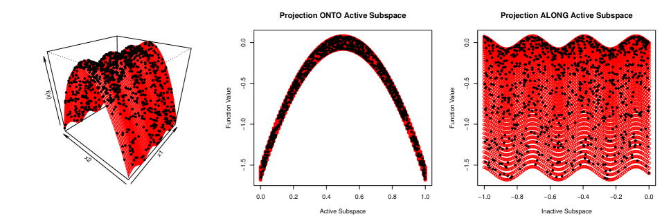
Figure 1: The 2-D function given by Equation (6) exhibits insignificant but high-frequency behavior in one dimension and significant but long-range behavior in the other. Filled black points are design points while red circles represent points evaluated on a regular grid for visualization. The ASM reveals a linear subspace along which most of the important changes occur (center), while the ARD principle would select the high-frequency dimension (right).

3.3 Quantifying the Uncertainty in C

Of perhaps equal importance as giving an estimate for $\mathbf{C}$ is quantifying uncertainty in that estimate. Given an estimate, Constantine, (2015) shows how the bootstrap method (Efron,, 1981) can be used to create intervals by applying parametric bootstrapping to simple methods used to estimate active subspaces (e.g., OLS, LL). However, application of the bootstrap to more sophisticated active subspace estimation methods such as the one presented in this article can lead to computational challenges. Instead, uncertainty of GP parameters can be propagated to uncertainty of $\mathbf{C}$ via a simple MC procedure. Myriad methods for quantifying GP hyperparameter uncertainty exist: a full posterior can be developed by using MCMC procedures, approximate posteriors can be determined (e.g., via variational methods), or the asymptotic normality of maximum likelihood estimators can be exploited. In light of its computational ease, the last method is explored here. This method involves computing the Hessian of the log likelihood at its maximum value, giving a covariance matrix for the parameters, and treating the maximizing parameter setting as the mean. This uncertainty on model parameters may be propagated to the active-subspace-defining singular values via MC: for each drawn parameter setting, estimate the singular values, then keep, for instance, the middle 95 percent of the draws. As an illustration, in Figure 2 we form intervals on the eigenvalues of the problem defined in (6). The downside of this approach is that, while it is speedy, it does not account for uncertainty as well as would a fully Bayesian approach leveraging MCMC.

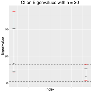
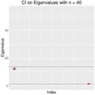
Figure 2: Eigenvalues from the problem in (6) are given interval estimates, expressing decreasing model uncertainty with samples of size 20 (left) and 40 (right). The Hessian expansion of the log-likelihood at its maximum gives a correlation of 0.16 between the two length-scale parameters. 95 and 99% confidence intervals are given in black and red, respectively, while the horizontal lines give the locations of the “true” eigenvalues estimated via classical MC techniques with 10,000 samples.

3.4 Acquisition Functions for Active Subspaces

Equipped with a closed-form GP estimate of $\mathbf{C}$ for a fixed design, we turn to the problem of choosing the next design to be evaluated given our observed responses so as to best learn about the active subspace. As do Labopin-Richard and Picheny, (2018), we take the approach of selecting the design that maximizes variance of our unknown quantity $\mathbf{C}$ at the next iteration. However, how to define this variance in our case is not clear. One could define subspace variance through ideas such as Fréchet variance (Fréchet,, 1948) and seek to minimize this, but the dimension of the active subspace is not known ahead of time, which would have to be determined by human observer or via a heuristic at each step of the sequential design process. Also possible is to consider measuring the variance of the spectral gap, which is problematic for the same reasons. We instead focus on the variance of the matrix $\mathbf{C}^{(n+1)}$, which we measure in three ways.

Since examination of $\mathbf{C}$’s spectrum is central to making decisions regarding the dimension of the active subspace, pinning down $\mathbf{C}$’s eigenvalues is of great interest. As such, we define the Trace acquisition function using the variance of the mean eigenvalue, which may be optimized by maximizing the variance of the trace of $\mathbf{C}^{(n+1)}$:

$$\texttt{Trace}=\mathbb{V}ar_{{\omega}}\left[\textrm{tr}(\mathbf{C}^{(n+1)})\right].$$

Of practical concern is that the Trace function may be calculated without computing the off-diagonal elements of the $\mathbf{C}$ matrix, which seems to some degree antithetical to the principle of ASMs seeking non-axis-aligned directions of importance.

We also consider two acquisition functions attempting to directly measure $\mathbf{C}$’s variance, which we term Var1,

$$\texttt{Var1}=\left\|\mathbb{E}_{{\omega}}\left[\left(\mathbf{C}^{(n+1)}-\mathbb{E}_{{\omega}}\left[\mathbf{C}^{(n+1)}\right]\right)\odot\left(\mathbf{C}^{(n+1)}-\mathbb{E}_{{\omega}}\left[\mathbf{C}^{(n+1)}\right]\right)\right]\right\|_{F}^{2},$$

and Var2,

$$\texttt{Var2}=\left\|\mathbb{E}_{{\omega}}\left[\left(\mathbf{C}^{(n+1)}-\mathbb{E}_{{\omega}}\left[\mathbf{C}^{(n+1)}\right]\right)\left(\mathbf{C}^{(n+1)}-\mathbb{E}_{{\omega}}\left[\mathbf{C}^{(n+1)}\right]\right)\right]\right\|_{F}^{2}.$$

Here, $\odot$ represents elementwise (Hadamard product) multiplication and $\|\mathbf{A}\|_{F}$ denotes the Frobenius norm of $\mathbf{A}$ (the root of the sum of its squared elements).

Of practical interest is that, again, closed-form expressions can be obtained for these three acquisition functions.

Theorem 4.

Given the coefficients $\beta_{i,j}(\tilde{\mathbf{x}})$ and $\gamma_{i,j}(\tilde{\mathbf{x}})$ from Theorem 3 stored in matrices $\mathbf{B}(\tilde{\mathbf{x}})$ and $\bm{\Gamma}(\tilde{\mathbf{x}})$, the acquisition functions and their gradients are available in the closed forms shown in Table 1.

Proof.

The derivation is detailed in Appendix C. ∎

We note further that $\mathbf{B}(\tilde{\mathbf{x}})$ and $\bm{\Gamma}(\tilde{\mathbf{x}})$ have closed-form expressions for popular kernels, including the Gaussian, Matérn 3/2, and Matérn 5/2; see Appendix A.

Table 1: Analytic expressions and gradients with respect to the new location $\tilde{\mathbf{x}}$ for each of our acquisition functions. For compactness, we employ $\mathbf{A}=\mathbf{C}^{(n+1)}-\mathbb{E}_{{\omega}}\left[\mathbf{C}^{(n+1)}\right]$. Dependence of $\mathbf{B}(\tilde{\mathbf{x}}),\partial\mathbf{B}(\tilde{\mathbf{x}}),\bm{\Gamma}(\tilde{\mathbf{x}})$, and $\partial\bm{\Gamma}(\tilde{\mathbf{x}})$ on $\tilde{\mathbf{x}}$ has been suppressed for brevity.

Name	Definition	Expression	d-Derivative
Trace	$\mathbb{V}ar_{{\omega}}\left[\textrm{tr}(\mathbf{C}^{(n+1)})\right]$	$\textrm{tr}(\mathbf{B}\odot\mathbf{B})+2\textrm{tr}(\bm{\Gamma}\odot\bm{\Gamma})$	$2\textrm{tr}(\partial\mathbf{B}_{d})\textrm{tr}(\mathbf{B})+4\textrm{tr}(\partial\bm{\Gamma}_{d}\textrm{tr}(\bm{\Gamma}))$
Var1	$\|\mathbb{E}_{{\omega}}\left[\mathbf{A}\odot\mathbf{A}\right]\|_{F}^{2}$	$\|\mathbf{B}\odot\mathbf{B}+2\bm{\Gamma}\odot\bm{\Gamma}\|_{F}^{2}$	$2(2\mathbf{B}\odot\partial\mathbf{B}_{d}+4\bm{\Gamma}\odot\partial\bm{\Gamma}_{d})\|\mathbf{B}\odot\mathbf{B}+2\bm{\Gamma}\odot\bm{\Gamma}|\|_{F}^{2}$
Var2	$\|\mathbb{E}_{{\omega}}\left[\mathbf{A}\mathbf{A}\right]\|_{F}^{2}$	$\|\mathbf{B}\mathbf{B}+2\bm{\Gamma}\bm{\Gamma}\|_{F}^{2}$	$2(\mathbf{B}\partial\mathbf{B}_{d}+\partial\mathbf{B}_{d}\mathbf{B}+2\bm{\Gamma}\partial\bm{\Gamma}_{d}+2\partial\bm{\Gamma}_{d}\bm{\Gamma})\|\mathbf{B}\mathbf{B}+2\bm{\Gamma}\bm{\Gamma}\|_{F}^{2}$

The details are given in the Appendix, where gradients are also discussed. A brief summary of the approach is given in Algorithm 1. The optimization with respect to $\tilde{\mathbf{x}}$ is non-convex; we pursue a multi-start approach by evaluating the acquisition function on a space filling design, then executing local searches via L-BFGS-B (Morales and Nocedal,, 2011) on the five points with the lowest acquisition function value.

Algorithm 1 Pseudocode for the sequential learning approach

1:$n_{0}$, criteria $J(\cdot)$ (e.g., Trace, Var1, Var2)

2:Construct and evaluate an initial design of experiments of size $n_{0}$ in $\mathcal{X}$

3:Build initial GP model

4:while time/evaluation budget not exhausted do

5:     Find $\tilde{\mathbf{x}}^{*}\in\arg\max_{\mathbf{x}\in\mathcal{X}}J(\mathbf{x})$

6:     Evaluate $f(\tilde{\mathbf{x}}^{*})$

7:     Update the GP model based on new data

8:end while

We now turn to application examples to demonstrate the benefits of sequential design for active subspace learning.

4 Numerical Experiments

We illustrate the advantage of judicious design-point selection by comparing sequential GP subspace estimation with random GP estimation and Monte Carlo estimation, as well as approaches using a global linear model (OLS) or local linear models (LL). The task at hand being estimation of a subspace, we measure error in a model’s prediction as the sine of the first principal angle between the true active subspace and the active subspace estimated at each potentially expensive function evaluation. The sine of the first principal angle between two subspaces $\mathcal{U}$ and $\hat{\mathcal{U}}$, denoted as $\angle_{1}{\mathcal{U}\hat{\mathcal{U}}}$, may be computed as the spectral norm of a simple expression of two unitary matrices, the first, $\mathbf{U}$, with range equal to $\mathcal{U}$ and the second, $\hat{\mathbf{U}}^{\perp}$, with kernel equal to $\hat{\mathcal{U}}$ (Ji-guang,, 1987, Lemma 3.1):

$$\sin\left(\angle_{1}{\mathcal{U}\hat{\mathcal{U}}}\right)=\left\|\mathbf{U}^{\top}\hat{\mathbf{U}}^{\perp}\right\|_{2}.$$ (7)

This “subspace distance” gives us some notion of the largest possible angle to be made between subspaces.

All of the tested methods begin with the same Latin hypercube sample and choose their next points either randomly or based on an acquisition function.

4.1 The Rank-1 Quadratic

We begin by learning a quadratic function defined by a rank-1 matrix $\mathbf{A}$; that is,

$$f(\mathbf{x})=\mathbf{x}^{\top}\mathbf{A}\mathbf{x}=\left(\mathbf{a}_{1}^{\top}\mathbf{x}\right)^{2},\mathbf{x}\in[0,1]^{m}$$ (8)

The gradient of this function is $\nabla f(\mathbf{x})=2\mathbf{A}\mathbf{x}=2\left(\mathbf{a}_{1}^{\top}\mathbf{x}\right)\mathbf{a}_{1}$, so gradients live entirely in the one-dimensional subspace given by the range of $\mathbf{A}$. During each trial, a vector $\mathbf{a}_{1}$ is generated with iid standard normal entries. The results of applying each algorithm to 50 randomly generated rank-1 $\mathbf{A}$ matrices in dimensions $m=$ 2, 5, and 8 are given in Figure 3. The initial design is 5 times the dimension of the space, and the number of points selected sequentially is 10 times the dimension, giving a total budget of 15 times the input dimension in terms of function evaluations. To simulate numerical error or a stochastic experiment, we rerun the experiments this time adding Gaussian noise to the objective with standard deviation $\tau=5e^{-5}$. In the noiseless case, as soon as we see one gradient, we have the active subspace, so finite differencing (simple forward differencing with a step size of $10^{-4}$) together with the Monte Carlo estimator gets the right answer after $m+1$ evaluations. With slight numerical noise, however, the accuracy obtained by finite differencing degrades, and the advantage of intelligent selection of evaluation points is clear.

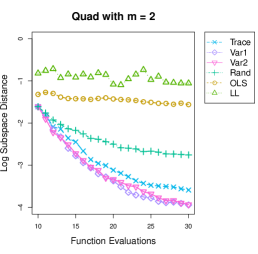
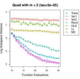
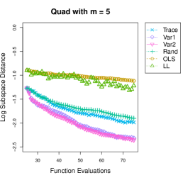
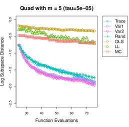
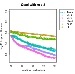
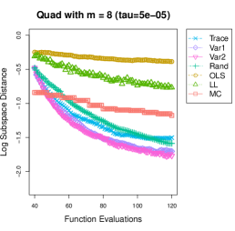
Figure 3: The quadratic problem (8) in dimensions 2, 5, and 8. The $x$-axis represents computational effort in function evaluations while the $y$-axis represents the log of the mean (based on 50 trials) of the subspace error. The standard Monte Carlo estimator has zero error after a single gradient evaluation modulo minimal numerical noise in the deterministic case, so is not pictured in column 1, but would be at $-\infty$ in theory and was found to be around $10^{-10}$ in practice.

The difference between the selected three definitions of variance of $\mathbf{C}^{(n+1)}$ can be observed in relation to the random infill, that is, randomly choosing the next point. Var1 and Var2 give similar results; Trace is in some cases barely better than random sampling. This indicates that to pinpoint the active subspace, it is insufficient to focus on the uncertainty associated with the mean (or sum) of the eigenvalues. Recall that each method begins with the exact same design, and thus that discrepancies in accuracy at the beginning of the simulation are due to how the methods differ in exploiting the same available data. Since the classical MC estimator cannot avail itself of random function evaluations, it is given that many additional function evaluations to conduct finite differencing prior to the trials that appear in the figures.

4.2 The Wing Weight Function

The wing weight function, introduced by Forrester et al., (2008), is a function of 10 inputs on a rectangular domain giving the weight of a light aircraft wing. Although it is a simple algebraic expression, it is of interest as a physically motivated test problem. Previously examined by the tutorial for the active_subspaces Python package, a prominent one-dimensional active subspace was discovered (see Figure 5). Here, we explore this function beginning with a design of 20 points and choose an additional 80 points via a sequential design policy or randomly. Since an analytic representation of the active subspace is unavailable, we measure the “true” active subspace by using finite differencing with the classical estimation technique with 10,000 function evaluations. Figure 4 illustrates the advantage of design-point selection via our acquisition criteria for smaller function evaluation budgets. The variances that account for non-axis-aligned terms of $\mathbf{C}^{(n+1)}$ (i.e., in contrast to the Trace acquisition function) perform best.

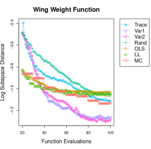
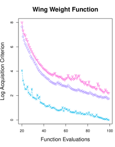
Figure 4: Results on a simulation on the wing weight function. Left: Function evaluations are represented with the $x$-axis, while subspace error at each iteration is shown on the $y$-axis. The advantage of sequential design for smaller function evaluation budgets is clear. Right: The value maximizing the acquisition function is given for sequential strategies at each iteration.

Figure 5: The log of the eigenvalues of $\mathbf{C}$ matrices estimated with many data. Gaps indicate potential cut-offs for the active subspace. The Wing Weight active subspace matrix was estimated via Finite Differencing on 10,000 random points. The Covid-19 active subspace matrix was estimated via our GP methodology with 2,000 points, as the simulator’s low accuracy precludes finite differencing. We chose active subspace dimensions of 1 and 3, respectively, as referenced in the experiments.

4.3 The Minnesota Covid-19 Simulator

The Minnesota Covid-19 Model (Enns et al.,, 2020) was developed to help guide public policy in response to the novel coronavirus, and calculates trajectories of various quantities of interest, such as cumulative death rates and ICU utilization over one year. However, the model depends on various epidemiological quantities, such as rate of asymptomatic infection, which are presently poorly understood. In this section, we treat this simulator as a black box and study the effect of varying certain parameters on the total covid-19 deaths. The cumulative number of deaths, though calculated as a continuous variable, is not sufficiently precise so as to allow finite differencing. Thus, in our simulations, accuracy is computed as compared to the active subspace given by a Gaussian process fit on 2,000 randomly sampled data (Figure 5 reveals that a three dimensional active subspace is reasonable). Figure 6 illustrates the performance of our three sequential design criteria as compared to a random baseline. Again the variance-based acquisition functions perform best, while the Trace function is in this case only marginally better than random.

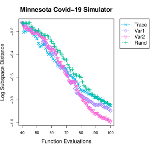
Figure 6: Comparison of GP based sequential design criteria on the Minnesota Covid-19 Simulator. Ground truth is taken to be the active subspace given by a GP with 2,000 randomly sampled input-output pairs. Left: Subspace error versus function evaluations, averaged over 40 runs. Right: Boxplots showing the final subspace error for each acquisition function over each of the 40 runs.

5 Discussion and Perspectives

In this article, we have shown that the surrogate-assisted estimation of active subspaces, a technique previously executed via Monte Carlo finite differencing, has a closed-form solution. This result was leveraged to create acquisition functions enabling evaluation-efficient estimation of such subspaces via sequential design, potentially saving (expensive) black-box evaluations. Although in this article we initialized our search with a standard Latin hypercube sample, choosing an initial design related to our acquisition criteria may be preferable, an issue we leave for future work. Active subspace methods being a field of active research, we leave the estimation via Gaussian processes of recent refinements, such as that proposed by Lee, (2019), for perspective. Future work could focus on problems specifically related to optimization, perhaps by considering a different measure to define the expected outer product of the gradient or by explicitly incorporating only those subspaces that play an important role in optimization, perhaps phrased in the framework of goal-oriented sensitivity analysis (Fort et al.,, 2016). Although not explored in this work, it is in principle straightforward to choose which points in the design space to explore in batches rather than one at a time. Such a problem, however, presents computational difficulty in optimization of the acquisition function. One may have to develop approximate methods in order for this to be carried out in practice.

SUPPLEMENTARY MATERIAL

Additional Kernel Expressions and Derivation:

Detailed update derivations and kernel expressions for Matérn 3/2 and 5/2 kernels as well as gradients for all kernel expressions. (PDF)

R-package for Sequential Active Subspace UQ:

R-package activegp containing code implementing methods described in this article (also available from CRAN). (GNU Tar file).

Appendix A Kernel Expressions

Here we provide specific formulae to evaluate $\int_{\mathcal{X}}\frac{\partial k(\mathbf{x},\mathbf{x}_{1})}{\partial x_{i}}\cdot\frac{\partial k(\mathbf{x}_{2},\mathbf{x})}{\partial x_{j}}d\mu(\mathbf{x})$, that is, the element $[\mathbf{W}_{i,j}]_{1,2}$ of the matrix $\mathbf{W}_{i,j}$ used in Theorem 2. Derivation of these formulae was aided by Wolfram Mathematica Wolfram Research, Inc, (2019). $[\mathbf{W}_{i,j}]_{1,2}$ may be written as a product of marginal functions as such if $i=j$:

$$[\mathbf{W}_{i,j}]_{1,2}=w_{i,i}([\mathbf{x}_{1}]_{i},[\mathbf{x}_{2}]_{i})\prod_{l=1,l\neq i}^{m}I_{l,l}([\mathbf{x}_{1}]_{l},[\mathbf{x}_{2}]_{l})$$

and, if $i\neq j$:

$$[\mathbf{W}_{i,j}]_{1,2}=w_{i,j}([\mathbf{x}_{1}]_{i},[\mathbf{x}_{2}]_{i})w_{i,j}([\mathbf{x}_{2}]_{j},[\mathbf{x}_{1}]_{j})\prod_{l=1,d\neq i,j}^{m}I_{l,l}([\mathbf{x}_{1}]_{l},[\mathbf{x}_{2}]_{l})$$

with

$$w_{i,i}(a,b)=\int_{0}^{1}\frac{\partial k(x,a)}{\partial x}\frac{\partial k(b,x)}{\partial x}dx$$

$$w_{i,j}(a,b)=\int_{0}^{1}\frac{\partial k(x,a)}{\partial x}k(b,x)dx$$

$$I_{d,d}(a,b)=\int_{0}^{1}k(x,a)k(b,x)dx.$$

Gradients of $\mathbf{W}_{i,j}$ with respect to designs (here, $\mathbf{x}_{1}$ or $\mathbf{x}_{2}$) are available by simply replacing the appropriate term in the product by its derivative.

Closed-form expressions and gradients are available for certain $k$. Expressions for the Gaussian, Matérn 3/2 and 5/2 kernels, and gradients may be found in the Supplementary Materials; and C++ code implementing all expressions is available in the R package activegp.

Appendix B Derivatives of the Updates

We want to express $\mathbf{C}^{(n+1)}$ as a function of $\mathbf{C}^{(n)}$, $\mathbf{x}_{n+1}$ and $y_{n+1}$. Ultimately we are also interested in its gradient. Reusing notations of Section 3.1, $C_{i,j}^{(n+1)}$ is composed of three parts, $E_{i,j}$, $tr(\mathbf{K}_{n+1}^{-1}\mathbf{W}_{i,j}^{(n+1)})$, and $\mathbf{y}_{n+1}^{\top}\mathbf{K}_{n+1}^{-1}\mathbf{W}_{i,j}^{(n+1)}\mathbf{K}_{n+1}^{-1}\mathbf{y}^{\top}_{n+1}$.

The first component is unchanged with the update. The second one can be derived by adapting results from Binois et al., (2019) since $\mathbf{W}_{i,j}^{(n+1)}$ may not be symmetric:

$$tr(\mathbf{K}_{n+1}^{-1}\mathbf{W}_{i,j}^{(n+1)})=tr(\mathbf{K}_{n}^{-1}\mathbf{W}_{i,j}^{(n)})-\sigma_{n}^{2}(\tilde{\mathbf{x}})\mathbf{g}(\tilde{\mathbf{x}})^{\top}\mathbf{W}_{i,j}^{(n)}\mathbf{g}(\tilde{\mathbf{x}})-(\mathbf{w}_{a}(\tilde{\mathbf{x}})+\mathbf{w}_{b}(\tilde{\mathbf{x}}))^{\top}\mathbf{g}(\tilde{\mathbf{x}})-\sigma_{n}^{2}(\tilde{\mathbf{x}})^{-1}w(\tilde{\mathbf{x}},\tilde{\mathbf{x}}).$$

For the remaining one, partition inverse equations (Barnett,, 1979) give

$$\mathbf{K}_{n+1}^{-1}=\begin{bmatrix}\mathbf{K}_{n}^{-1}+\mathbf{g}(\tilde{\mathbf{x}})\mathbf{g}(\tilde{\mathbf{x}})^{\top}\sigma_{n}^{2}(\tilde{\mathbf{x}})&\mathbf{g}(\tilde{\mathbf{x}})\\ \mathbf{g}(\tilde{\mathbf{x}})^{\top}&\sigma_{n}^{2}(\tilde{\mathbf{x}})^{-1}\end{bmatrix},$$

where $\mathbf{g}(\tilde{\mathbf{x}})=-\sigma_{n}^{2}(\tilde{\mathbf{x}})^{-1}\mathbf{K}_{n}^{-1}\mathbf{k}_{n}(\tilde{\mathbf{x}})$ and $\sigma^{2}_{n}(\tilde{\mathbf{x}})=k_{n}(\tilde{\mathbf{x}},\tilde{\mathbf{x}})$ as in (5). Denote $\mathbf{G}=\mathbf{g}(\tilde{\mathbf{x}})\mathbf{g}(\tilde{\mathbf{x}})^{\top}\sigma_{n}^{2}(\tilde{\mathbf{x}})$.

Decomposing and regrouping terms, we get the following.

$$\begin{bmatrix}\mathbf{y}_{n}^{\top}&y_{n+1}\end{bmatrix}\begin{bmatrix}\mathbf{K}_{n}^{-1}+\mathbf{G}&\mathbf{g}(\tilde{\mathbf{x}})\\ \mathbf{g}(\tilde{\mathbf{x}})^{\top}&\sigma_{n}^{2}(\tilde{\mathbf{x}})^{-1}\end{bmatrix}\begin{bmatrix}\mathbf{W}_{i,j}^{(n)}&\mathbf{w}_{a}(\tilde{\mathbf{x}})\\ \mathbf{w}_{b}(\tilde{\mathbf{x}})^{\top}&w(\tilde{\mathbf{x}},\tilde{\mathbf{x}})\end{bmatrix}\begin{bmatrix}\mathbf{K}_{n}^{-1}+\mathbf{G}&\mathbf{g}(\tilde{\mathbf{x}})\\ \mathbf{g}(\tilde{\mathbf{x}})^{\top}&\sigma_{n}^{2}(\tilde{\mathbf{x}})^{-1}\end{bmatrix}\begin{bmatrix}\mathbf{y}_{n}\\ y_{n+1}\end{bmatrix}$$

$$=\begin{bmatrix}\mathbf{y}_{n}^{\top}(\mathbf{K}_{n}^{-1}+\mathbf{G})+y_{n+1}\mathbf{g}(\tilde{\mathbf{x}})^{\top}&\mathbf{y}_{n}^{\top}\mathbf{g}(\tilde{\mathbf{x}})+y_{n+1}\sigma_{n}^{2}(\tilde{\mathbf{x}})^{-1}\end{bmatrix}\mathbf{W}_{i,j}^{(n+1)}\begin{bmatrix}(\mathbf{K}_{n}^{-1}+\mathbf{G})\mathbf{y}_{n}+y_{n+1}\mathbf{g}(\tilde{\mathbf{x}})\\ \mathbf{g}(\tilde{\mathbf{x}})^{\top}\mathbf{y}_{n}+y_{n+1}\sigma_{n}^{2}(\tilde{\mathbf{x}})^{-1}\end{bmatrix}$$

$$= \mathbf{y}_{n}^{\top}(\mathbf{K}_{n}^{-1}+\mathbf{G})\mathbf{W}_{i,j}^{(n)}(\mathbf{K}_{n}^{-1}+\mathbf{G})\mathbf{y}_{n}+y_{n+1}\mathbf{y}_{n}^{\top}(\mathbf{K}_{n}^{-1}+\mathbf{G})\mathbf{W}_{i,j}^{(n)}\mathbf{g}(\tilde{\mathbf{x}})+y_{n+1}\mathbf{g}(\tilde{\mathbf{x}})^{\top}\mathbf{W}_{i,j}^{(n)}(\mathbf{K}_{n}^{-1}+\mathbf{G})\mathbf{y}_{n}$$

$$+y_{n+1}^{2}\mathbf{g}(\tilde{\mathbf{x}})^{\top}\mathbf{W}_{i,j}^{(n)}\mathbf{g}(\tilde{\mathbf{x}})+\mathbf{y}_{n}^{\top}\mathbf{g}(\tilde{\mathbf{x}})\mathbf{w}_{b}(\tilde{\mathbf{x}})^{\top}(\mathbf{K}_{n}^{-1}+\mathbf{G})\mathbf{y}_{n}+\mathbf{y}_{n}^{\top}\mathbf{g}(\tilde{\mathbf{x}})\mathbf{w}_{b}(\tilde{\mathbf{x}})^{\top}\mathbf{g}(\tilde{\mathbf{x}})y_{n+1}$$

$$+y_{n+1}\sigma_{n}^{2}(\tilde{\mathbf{x}})^{-1}\mathbf{w}_{b}(\tilde{\mathbf{x}})^{\top}(\mathbf{K}_{n}^{-1}+\mathbf{G})\mathbf{y}_{n}+y_{n+1}^{2}\sigma_{n}^{2}(\tilde{\mathbf{x}})^{-1}\mathbf{w}_{b}(\tilde{\mathbf{x}})^{\top}\mathbf{g}(\tilde{\mathbf{x}})$$

$$+\mathbf{y}_{n}^{\top}(\mathbf{K}_{n}^{-1}+\mathbf{G})\mathbf{w}_{a}(\tilde{\mathbf{x}})\mathbf{g}(\tilde{\mathbf{x}})^{\top}\mathbf{y}_{n}+y_{n+1}\sigma_{n}^{2}(\tilde{\mathbf{x}})^{-1}\mathbf{y}_{n}^{\top}(\mathbf{K}_{n}^{-1}+\mathbf{G})\mathbf{w}_{a}(\tilde{\mathbf{x}})+y_{n+1}\mathbf{g}(\tilde{\mathbf{x}})^{\top}\mathbf{w}_{a}(\tilde{\mathbf{x}})\mathbf{g}(\tilde{\mathbf{x}})^{\top}\mathbf{y}_{n}$$

$$+y_{n+1}^{2}\sigma_{n}^{2}(\tilde{\mathbf{x}})^{-1}\mathbf{g}(\tilde{\mathbf{x}})^{\top}\mathbf{w}_{a}(\tilde{\mathbf{x}})+w(\tilde{\mathbf{x}},\tilde{\mathbf{x}})\mathbf{y}_{n}^{\top}\mathbf{g}(\tilde{\mathbf{x}})\mathbf{g}(\tilde{\mathbf{x}})^{\top}\mathbf{y}_{n}+w(\tilde{\mathbf{x}},\tilde{\mathbf{x}})y_{n+1}\sigma_{n}^{2}(\tilde{\mathbf{x}})^{-1}\mathbf{y}_{n}^{\top}\mathbf{g}(\tilde{\mathbf{x}})$$

$$+y_{n+1}\sigma_{n}^{2}(\tilde{\mathbf{x}})^{-1}w(\tilde{\mathbf{x}},\tilde{\mathbf{x}})\mathbf{g}(\tilde{\mathbf{x}})^{\top}\mathbf{y}_{n}+y_{n+1}^{2}\sigma_{n}^{2}(\tilde{\mathbf{x}})^{-2}w(\tilde{\mathbf{x}},\tilde{\mathbf{x}})$$

After replacing $\mathbf{G}$ and $\mathbf{g}$ by their expressions and factoring, we get the expression for $C_{i,j}^{(n+1)}-C_{i,j}^{(n)}=$

$$-(\mathbf{w}_{a}(\tilde{\mathbf{x}})+\mathbf{w}_{b}(\tilde{\mathbf{x}}))^{\top}\mathbf{g}(\tilde{\mathbf{x}})$$

$$-(\mathbf{y}_{n}^{\top}\mathbf{g}(\tilde{\mathbf{x}})+y_{n+1}\sigma_{n}^{2}(\tilde{\mathbf{x}})^{-1})\left[\mathbf{y}_{n}^{\top}\mathbf{K}_{n}^{-1}\mathbf{W}_{i,j}^{(n)}\mathbf{K}_{n}^{-1}\mathbf{k}_{n}(\tilde{\mathbf{x}})+\mathbf{k}_{n}(\tilde{\mathbf{x}})^{\top}\mathbf{K}_{n}^{-1}\mathbf{W}_{i,j}^{(n)}\mathbf{K}_{n}^{-1}\mathbf{y}_{n}\right]$$

$$+(\mathbf{y}_{n}^{\top}\mathbf{g}(\tilde{\mathbf{x}})+y_{n+1}\sigma_{n}^{2}(\tilde{\mathbf{x}})^{-1})(\mathbf{w}_{a}(\tilde{\mathbf{x}})+\mathbf{w}_{b}(\tilde{\mathbf{x}}))^{\top}(\mathbf{K}_{n}^{-1}\mathbf{y}_{n}+\mathbf{g}(\tilde{\mathbf{x}})y_{n+1}-\mathbf{g}(\tilde{\mathbf{x}})\mathbf{k}_{n}(\tilde{\mathbf{x}})^{\top}\mathbf{K}_{n}^{-1}\mathbf{y}_{n})$$

$$+\left[(\mathbf{y}_{n}^{\top}\mathbf{g}(\tilde{\mathbf{x}})+y_{n+1}\sigma_{n}^{2}(\tilde{\mathbf{x}})^{-1})^{2}-\sigma_{n}^{2}(\tilde{\mathbf{x}})^{-1}\right]\left[w(\tilde{\mathbf{x}},\tilde{\mathbf{x}})+\mathbf{k}_{n}(\tilde{\mathbf{x}})^{\top}\mathbf{K}_{n}^{-1}\mathbf{W}_{i,j}^{(n)}\mathbf{K}_{n}^{-1}\mathbf{k}_{n}(\tilde{\mathbf{x}})\right].$$

Appendix C Infill Criteria Derivation

At step $n$, $y_{n+1}\sim\mathcal{N}(m_{n}(\tilde{\mathbf{x}}),\sigma_{n}^{2}(\tilde{\mathbf{x}}))$. Taking the expectation with respect to $y_{n+1}$ considerably simplify the expressions:

$$\mathbb{E}_{\omega}\left[C_{i,j}^{(n+1)}|\mathcal{A}_{n}\right]=C_{i,j}^{(n)}$$

$$\mathbb{V}ar_{\omega}\left[C_{i,j}^{(n+1)}|\mathcal{A}_{n}\right]=\beta^{2}+2\gamma^{2},$$

where expressions for $\beta$ and $\gamma$ are given below. Indeed:
1) $\mathbb{E}_{\omega}\left[\mathbf{y}_{n}^{\top}\mathbf{g}(\tilde{\mathbf{x}})+y_{n+1}\sigma_{n}^{2}(\tilde{\mathbf{x}})^{-1}\right]=(\mathbf{y}_{n}^{\top}\mathbf{g}(\tilde{\mathbf{x}})+m_{n}(\tilde{\mathbf{x}})\sigma_{n}^{2}(\tilde{\mathbf{x}})^{-1})=0$ by definition of $\mathbf{g}(\tilde{\mathbf{x}})$
2) $\mathbb{E}_{\omega}\left[(\mathbf{y}_{n}^{\top}\mathbf{g}(\tilde{\mathbf{x}})+y_{n+1}\sigma_{n}^{2}(\tilde{\mathbf{x}})^{-1})^{2}\right]=\sigma_{n}^{2}(\tilde{\mathbf{x}})^{-2}m_{n}(\tilde{\mathbf{x}})-2\sigma_{n}^{2}(\tilde{\mathbf{x}})^{-2}m_{n}(\tilde{\mathbf{x}})^{2}+\sigma_{n}^{2}(\tilde{\mathbf{x}})^{-2}(m_{n}(\tilde{\mathbf{x}})^{2}+\sigma_{n}^{2}(\tilde{\mathbf{x}}))=\sigma_{n}^{2}(\tilde{\mathbf{x}})^{-1}$
3) $\mathbb{E}_{\omega}\left[y_{n+1}(\mathbf{y}_{n}^{\top}\mathbf{g}(\tilde{\mathbf{x}})+y_{n+1}\sigma_{n}^{2}(\tilde{\mathbf{x}})^{-1})\right]=-m_{n}(\tilde{\mathbf{x}})^{2}\sigma_{n}^{2}(\tilde{\mathbf{x}})^{-1}+\sigma_{n}^{2}(\tilde{\mathbf{x}})^{-1}(m_{n}(\tilde{\mathbf{x}})^{2}+\sigma_{n}^{2}(\tilde{\mathbf{x}}))=1$.

Notice that if we use the plugin estimator of $y_{n+1}$, namely, $m_{n}(\tilde{\mathbf{x}})$, then

$$\hat{C}_{i,j}^{(n+1)}=C_{i,j}^{(n)}-\left(\sigma_{n}^{2}(\tilde{\mathbf{x}})^{-1}\mathbf{k}_{n}(\tilde{\mathbf{x}})^{\top}\mathbf{K}_{n}^{-1}\mathbf{W}_{i,j}^{(n)}\mathbf{K}_{n}^{-1}\mathbf{k}_{n}(\tilde{\mathbf{x}})+(\mathbf{w}_{a}(\tilde{\mathbf{x}})+\mathbf{w}_{b}(\tilde{\mathbf{x}}))^{\top}\mathbf{g}(\tilde{\mathbf{x}})+\sigma_{n}^{2}(\tilde{\mathbf{x}})^{-1}w(\tilde{\mathbf{x}},\tilde{\mathbf{x}})\right),$$

which reduces to the integrated mean square prediction error of the corresponding derivatives.

For further simplifications, denote by $Z=\frac{y_{n+1}-m_{n}(\tilde{\mathbf{x}})}{\sigma_{n}(\tilde{\mathbf{x}})}$ a $\mathcal{N}(0,1)$ random variable.

Then $C_{i,j}^{(n+1)}-C_{i,j}^{(n)}$ can be rewritten as

$$-(\mathbf{w}_{a}(\tilde{\mathbf{x}})+\mathbf{w}_{b}(\tilde{\mathbf{x}}))^{\top}\mathbf{g}(\tilde{\mathbf{x}})-\sigma^{2}_{n}(\tilde{\mathbf{x}})^{-1}\left[w(\tilde{\mathbf{x}},\tilde{\mathbf{x}})+\mathbf{k}_{n}(\tilde{\mathbf{x}})^{\top}\mathbf{K}_{n}^{-1}\mathbf{W}_{i,j}^{(n)}\mathbf{K}_{n}^{-1}\mathbf{k}_{n}(\tilde{\mathbf{x}})\right]$$

$$+Z\sigma_{n}(\tilde{\mathbf{x}})^{-1}\left[\mathbf{y}_{n}^{\top}\mathbf{K}_{n}^{-1}\mathbf{W}_{i,j}^{(n)}\mathbf{K}_{n}^{-1}\mathbf{k}_{n}(\tilde{\mathbf{x}})+\mathbf{k}_{n}(\tilde{\mathbf{x}})^{\top}\mathbf{K}_{n}^{-1}\mathbf{W}_{i,j}^{(n)}\mathbf{K}_{n}^{-1}\mathbf{y}_{n}-(\mathbf{w}_{a}(\tilde{\mathbf{x}})+\mathbf{w}_{b}(\tilde{\mathbf{x}}))^{\top}\mathbf{K}_{n}^{-1}\mathbf{y}_{n}\right]$$

$$+Z^{2}\sigma_{n}^{2}(\tilde{\mathbf{x}})^{-1}\left[w(\tilde{\mathbf{x}},\tilde{\mathbf{x}})+\mathbf{k}_{n}(\tilde{\mathbf{x}})^{\top}\mathbf{K}_{n}^{-1}\mathbf{W}_{i,j}^{(n)}\mathbf{K}_{n}^{-1}\mathbf{k}_{n}(\tilde{\mathbf{x}})-(\mathbf{w}_{a}(\tilde{\mathbf{x}})+\mathbf{w}_{b}(\tilde{\mathbf{x}}))^{\top}\mathbf{K}_{n}^{-1}\mathbf{k}_{n}(\tilde{\mathbf{x}})\right].$$

Now denote the coefficient to the linear $Z$ term as $\beta_{i,j}$ and that to the quadratic $Z$ term as $\gamma_{i,j}$, and further denote the matrices containing these as entries given $\tilde{\mathbf{x}}$ as $\mathbf{B}(\tilde{\mathbf{x}})$ and $\bm{\Gamma}(\tilde{\mathbf{x}})$, respectively. We further define 3D arrays $\partial\mathbf{B}(\tilde{\mathbf{x}})$ and $\partial\bm{\Gamma}(\tilde{\mathbf{x}})$ such that $\partial\mathbf{B}(\tilde{\mathbf{x}})_{d}$ gives a matrix of derivatives of each element of $\mathbf{B}(\tilde{\mathbf{x}})$ with respect to the $d$th element of $\tilde{\mathbf{x}}$:

$$\partial\mathbf{B}(\tilde{\mathbf{x}})_{d}=\mathbf{y}_{n}^{\top}\mathbf{K}_{n}^{-1}(\mathbf{W}_{i,j}^{(n)}+(\mathbf{W}_{i,j}^{(n)})^{\top})\mathbf{K}_{n}^{-1}\bm{\kappa}_{d}(\tilde{\mathbf{x}})^{\top}-\mathbf{y}_{n}^{\top}\mathbf{K}_{n}^{-1}\left(\frac{\partial\mathbf{w}_{a}(\tilde{\mathbf{x}})}{\partial\tilde{\mathbf{x}}_{d}}+\frac{\partial\mathbf{w}_{b}(\tilde{\mathbf{x}})}{\partial\tilde{\mathbf{x}}_{d}}\right)-\mathbf{B}\frac{\partial\sigma_{n}(\tilde{\mathbf{x}})}{\partial\tilde{\mathbf{x}}_{d}}\sigma_{n}(\tilde{\mathbf{x}})^{-\frac{1}{2}}$$

and

$$\partial\bm{\Gamma}(\tilde{\mathbf{x}})_{d}=\sigma_{n}^{-1}(\tilde{\mathbf{x}})\Big{(}\frac{\partial w(\tilde{\mathbf{x}},\tilde{\mathbf{x}})}{\tilde{\mathbf{x}}_{d}}^{\top}+\mathbf{k}_{n}(\tilde{\mathbf{x}})^{\top}\mathbf{K}_{n}^{-1}(\mathbf{W}_{i,j}^{(n)}+(\mathbf{W}_{i,j}^{(n)})^{\top})\mathbf{K}_{n}^{-1}\bm{\kappa}_{d}(\tilde{\mathbf{x}})^{\top}-\\ \mathbf{k}_{n}(\tilde{\mathbf{x}})^{\top}\mathbf{K}_{n}^{-1}\left(\frac{\partial\mathbf{w}_{a}(\tilde{\mathbf{x}})}{\partial\tilde{\mathbf{x}}_{d}}+\frac{\partial\mathbf{w}_{b}(\tilde{\mathbf{x}})}{\partial\tilde{\mathbf{x}}_{d}}\right)-(\mathbf{w}_{a}(\tilde{\mathbf{x}})+\mathbf{w}_{b}(\tilde{\mathbf{x}}))^{\top}\mathbf{K}_{n}^{-1}\frac{\partial w(\tilde{\mathbf{x}},\tilde{\mathbf{x}})}{\tilde{\mathbf{x}}_{d}}-\frac{\partial\sigma_{n}(\tilde{\mathbf{x}})}{\partial\tilde{\mathbf{x}}_{d}}\bm{\Gamma}\Big{)}.$$

We are now equipped to derive closed-form expressions for our infill criteria, as well as gradients of those expressions with respect to design locations, the results of which are given in Table 1.

The submitted manuscript has been created by UChicago Argonne, LLC, Operator of Argonne National Laboratory (“Argonne”). Argonne, a U.S. Department of Energy Office of Science laboratory, is operated under Contract No. DE-AC02-06CH11357. The U.S. Government retains for itself, and others acting on its behalf, a paid-up nonexclusive, irrevocable worldwide license in said article to reproduce, prepare derivative works, distribute copies to the public, and perform publicly and display publicly, by or on behalf of the Government. The Department of Energy will provide public access to these results of federally sponsored research in accordance with the DOE Public Access Plan. http://energy.gov/downloads/doe-public-access-plan.

References

- Barnett, (1979) Barnett, S. (1979). Matrix Methods for Engineers and Scientists. McGraw-Hill.
- Bellman, (2003) Bellman, R. E. (2003). Dynamic Programming. New York, NY: Dover Publications.
- Binois et al., (2019) Binois, M., Huang, J., Gramacy, R. B., and Ludkovski, M. (2019). “Replication or Exploration? Sequential Design for Stochastic Simulation Experiments.” Technometrics, 61, 1, 7–23.
- Constantine, (2015) Constantine, P. G. (2015). Active Subspaces. Philadelphia, PA: SIAM.
- Constantine et al., (2014) Constantine, P. G., Dow, E., and Wang, Q. (2014). “Active Subspace Methods in Theory and Practice: Applications to Kriging Surfaces.” SIAM Journal on Scientific Computing, 36, 4, A1500–A1524.
- Constantine et al., (2017) Constantine, P. G., Eftekhari, A., Hokanson, J., and Ward, R. A. (2017). “A Near-Stationary Subspace for Ridge Approximation.” Computer Methods in Applied Mechanics and Engineering, 326, 402–421.
- Constantine et al., (2015) Constantine, P. G., Eftekhari, A., and Wakin, M. B. (2015). “Computing Active Subspaces Efficiently with Gradient Sketching.” In 2015 IEEE 6th International Workshop on Computational Advances in Multi-Sensor Adaptive Processing (CAMSAP), 353–356. IEEE.
- De Lozzo and Marrel, (2016) De Lozzo, M. and Marrel, A. (2016). “Estimation of the Derivative-Based Global Sensitivity Measures Using a Gaussian Process Metamodel.” SIAM/ASA Journal on Uncertainty Quantification, 4, 1, 708–738.
- Djolonga et al., (2013) Djolonga, J., Krause, A., and Cevher, V. (2013). “High-Dimensional Gaussian Process Bandits.” In Advances in Neural Information Processing Systems 26, 1025–1033.
- Durrande et al., (2012) Durrande, N., Ginsbourger, D., and Roustant, O. (2012). “Additive Kernels for Gaussian Process Modeling.” Annales de la Facultée de Sciences de Toulouse, 17.
- Durrande et al., (2013) Durrande, N., Ginsbourger, D., Roustant, O., and Carraro, L. (2013). “ANOVA Kernels and RKHS of Zero Mean Functions for Model-Based Sensitivity Analysis.” Journal of Multivariate Analysis, 115, 57–67.
- Duvenaud et al., (2011) Duvenaud, D. K., Nickisch, H., and Rasmussen, C. E. (2011). “Additive Gaussian Processes.” In Advances in Neural Information Processing Systems 24, eds. J. Shawe-Taylor, R. S. Zemel, P. L. Bartlett, F. Pereira, and K. Q. Weinberger, 226–234. Curran Associates, Inc.
- Efron, (1981) Efron, B. (1981). “Nonparametric Estimates of Standard Error: The Jackknife, the Bootstrap and Other Methods.” Biometrika, 68, 3, 589–599.
- Enns et al., (2020) Enns, E. A., Kirkeide, M., Mehta, A., MacLehose, R., Knowlton, G. S., Smith, M. K., Searle, K. M., Zhao, R., Gildemeister, S., Simon, A., Sanstead, E., and Kulasingam, S. (2020). “Modeling the Impact of Social Distancing Measures on the Spread of SARS-CoV-2 in Minnesota.” Tech. Rep. 1148-427724, University of Minnesota.
- Forrester et al., (2008) Forrester, A. I. J., Sobester, A., and Keane, A. J. (2008). Engineering Design via Surrogate Modelling - A Practical Guide. Wiley.
- Fort et al., (2016) Fort, J.-C., Klein, T., and Rachdi, N. (2016). “New Sensitivity Analysis Subordinated to a Contrast.” Communications in Statistics - Theory and Methods, 45, 15, 4349–4364.
- Fréchet, (1948) Fréchet, M. R. (1948). “Les Éléments Aléatoires de Nature Quelconque dans un Espace Distancié.” Annales de l’Institut Henri Poincaré, 10, 4, 215–310.
- Friedman and Stuetzle, (1981) Friedman, J. H. and Stuetzle, W. (1981). “Projection Pursuit Regression.” Journal of the American Statistical Association, 76, 376, 817–823.
- Fukumizu and Leng, (2014) Fukumizu, K. and Leng, C. (2014). “Gradient-Based Kernel Dimension Reduction for Regression.” Journal of the American Statistical Association, 109, 505, 359–370.
- Garnett et al., (2014) Garnett, R., Osborne, M. A., and Hennig, P. (2014). “Active Learning of Linear Embeddings for Gaussian Processes.” In Proceedings of the Thirtieth Conference on Uncertainty in Artificial Intelligence, UAI’14, 230–239. AUAI Press.
- Ghosh, (2018) Ghosh, S. (2018). Kernel Smoothing: Principles, Methods and Applications. John Wiley & Sons.
- Glaws et al., (2020) Glaws, A., Constantine, P. G., and Cook, R. D. (2020). “Inverse regression for ridge recovery: a data-driven approach for parameter reduction in computer experiments.” Statistics and Computing, 30, 2, 237–253.
- Hokanson and Constantine, (2018) Hokanson, J. and Constantine, P. G. (2018). “Data-Driven Polynomial Ridge Approximation Using Variable Projection.” SIAM Journal on Scientific Computing, 40, 3, A1566–A1589.
- Holodnak et al., (2018) Holodnak, J. T., Ipsen, I. C., and Smith, R. C. (2018). “A Probabilistic Subspace Bound with Application to Active Subspaces.” SIAM Journal on Matrix Analysis and Applications, 39, 3, 1208–1220.
- Iooss and Lemaître, (2015) Iooss, B. and Lemaître, P. (2015). “A Review on Global Sensitivity Analysis Methods.” In Uncertainty Management in Simulation-Optimization of Complex Systems: Algorithms and Applications, eds. C. Meloni and G. Dellino, 101–122. Springer.
- Ji-guang, (1987) Ji-guang, S. (1987). “Perturbation of Angles between Linear Subspaces.” Journal of Computational Mathematics, 5, 1, 58–61.
- Labopin-Richard and Picheny, (2018) Labopin-Richard, T. and Picheny, V. (2018). “Sequential Design of Experiments for Estimating Percentiles of Black-Box Functions.” Statistica Sinica, 28, 853–877.
- Larson et al., (2019) Larson, J., Menickelly, M., and Wild, S. M. (2019). “Derivative-Free Optimization Methods.” Acta Numerica, 28, 287–404.
- Lee, (2019) Lee, M. R. (2019). “Modified Active Subspaces Using the Average of Gradients.” SIAM/ASA Journal on Uncertainty Quantification, 7, 1, 53–66.
- Li, (1991) Li, K.-C. (1991). “Sliced Inverse Regression for Dimension Reduction.” Journal of the American Statistical Association, 86, 414, 316–327.
- Li, (1992) — (1992). “On Principal Hessian Directions for Data Visualization and Dimension Reduction: Another Application of Stein’s Lemma.” Journal of the American Statistical Association, 87, 420, 1025–1039.
- Li et al., (2016) Li, W., Lin, G., and Li, B. (2016). “Inverse regression-based uncertainty quantification algorithms for high-dimensional models: Theory and practice.” Journal of Computational Physics, 321, 259 – 278.
- Ma and Zhu, (2013) Ma, Y. and Zhu, L. (2013). “A Review on Dimension Reduction.” International Statistical Review, 81, 1, 134–150.
- Marcy, (2017) Marcy, P. W. (2017). “Bayesian Gaussian Process Models on Spaces of Sufficient Dimension Reduction.” Statistical Perspectives of Uncertainty Quantification Workshop.
- Morales and Nocedal, (2011) Morales, J. L. and Nocedal, J. (2011). “Remark on “Algorithm 778: L-BFGS-B: Fortran Subroutines for Large-Scale Bound Constrained Optimization”.” ACM Transactions on Mathematical Software, 38, 1, 1–4.
- Moré and Wild, (2012) Moré, J. J. and Wild, S. M. (2012). “Estimating Derivatives of Noisy Simulations.” ACM Transactions on Mathematical Software, 38, 3, 19:1–19:21.
- Namura et al., (2017) Namura, N., Shimoyama, K., and Obayashi, S. (2017). “Kriging Surrogate Model with Coordinate Transformation Based on Likelihood and Gradient.” Journal of Global Optimization, 68, 4, 827–849.
- Othmer et al., (2016) Othmer, C., Lukaczyk, T. W., Constantine, P., and Alonso, J. J. (2016). “On Active Subspaces in Car Aerodynamics.” In 17th AIAA/ISSMO Multidisciplinary Analysis and Optimization Conference. American Institute of Aeronautics and Astronautics.
- Palar and Shimoyama, (2017) Palar, P. S. and Shimoyama, K. (2017). “Exploiting Active Subspaces in Global Optimization: How Complex is Your Problem?” In Proceedings of the Genetic and Evolutionary Computation Conference Companion on - GECCO ’17, 1487–1494. ACM Press.
- Palar and Shimoyama, (2018) — (2018). “On The Accuracy of Kriging Model in Active Subspaces.” In 2018 AIAA/ASCE/AHS/ASC Structures, Structural Dynamics, and Materials Conference, 0913.
- Petersen et al., (2008) Petersen, K. B., Pedersen, M. S., et al. (2008). “The Matrix Cookbook.” Technical University of Denmark, 7, 15.
- Rasmussen and Williams, (2006) Rasmussen, C. E. and Williams, C. (2006). Gaussian Processes for Machine Learning. MIT Press.
- Salem et al., (2019) Salem, M. B., Bachoc, F., Roustant, O., Gamboa, F., and Tomaso, L. (2019). “Sequential Dimension Reduction for Learning Features of Expensive Black-Box Functions.” Preprint 01688329v2, HAL.
- Samarov, (1993) Samarov, A. M. (1993). “Exploring Regression Structure Using Nonparametric Functional Estimation.” Journal of the American Statistical Association, 88, 423, 836–847.
- Scholkopf and Smola, (2001) Scholkopf, B. and Smola, A. J. (2001). Learning with Kernels: Support Vector Machines, Regularization, Optimization, and Beyond. Cambridge, MA: MIT Press.
- Sobol, (2001) Sobol, I. (2001). “Global Sensitivity Indices for Nonlinear Mathematical Models and Their Monte Carlo Estimates.” Mathematics and Computers in Simulation, 55, 1, 271–280. The Second IMACS Seminar on Monte Carlo Methods.
- Sung et al., (2019) Sung, C.-L., Wang, W., Plumlee, M., and Haaland, B. (2019). “Multiresolution Functional ANOVA for Large-Scale, Many-Input Computer Experiments.” Journal of the American Statistical Association, 115, 530, 908–919.
- Titsias and Lawrence, (2010) Titsias, M. and Lawrence, N. D. (2010). “Bayesian Gaussian Process Latent Variable Model.” In Proceedings of the Thirteenth International Conference on Artificial Intelligence and Statistics, 844–851.
- Tripathy et al., (2016) Tripathy, R., Bilionis, I., and Gonzalez, M. (2016). “Gaussian Processes with Built-in Dimensionality Reduction: Applications to High-Dimensional Uncertainty Propagation.” Journal of Computational Physics, 321, 191–223.
- Viswanath et al., (2011) Viswanath, A., J. Forrester, A., and Keane, A. (2011). “Dimension Reduction for Aerodynamic Design Optimization.” AIAA Journal, 49, 6, 1256–1266.
- Vivarelli and Williams, (1999) Vivarelli, F. and Williams, C. K. I. (1999). “Discovering Hidden Features with Gaussian Processes Regression.” In Proceedings of the 1998 Conference on Advances in Neural Information Processing Systems II, 613–619. MIT Press.
- Wang et al., (2016) Wang, Z., Hutter, F., Zoghi, M., Matheson, D., and De Freitas, N. (2016). “Bayesian Optimization in a Billion Dimensions via Random Embeddings.” Journal of Artificial Intelligence Research, 55, 1, 361–387.
- Wolfram Research, Inc, (2019) Wolfram Research, Inc (2019). “Mathematica, Version 12.0.” Champaign, IL, 2019.