Radiative neutrino model with semi-annihilation dark matter

Abstract

We propose a Two-Loop induced radiative neutrino model with hidden gauged $U(1)$ symmetry, in which a dark matter of Dirac fermion arises. The relic density gets contribution from annihilation and semi-annihilation due to a residual $\mathbb{Z}_{3}$ parity. After imposing the requirement of neutrino oscillation data and lepton flavour violation bounds, we find out that the semi-annihilation plays a crucial role in order to satisfy the relic density constraint $0.117<\Omega h^{2}<0.123$, by proceeding near either one of two deconstructive scalar resonances. Our numerical analysis demonstrates the allowed region for the DM-Scalar coupling with the DM mass in $(80,400)$ GeV.

I Introduction

Radiative seesaw neutrino models are one of the attractive scenarios to connect neutrino sector with dark matter (DM) sector in a natural manner. These two sectors certainly involve mysterious puzzles that are frequently interpreted as physics beyond the Standard Model (SM). When the neutrino masses are radiatively induced, the magnitude of relevant couplings could reach $\mathcal{O}(1)$ compared with the case where the neutrino mass is generated at the tree-level, so that the mass hierarchy among the SM sector and heavy fermion/scalar sectors is largely alleviated. Furthermore, new particles that are accommodated in the theory are at $\mathcal{O}$(TeV) energy scale and accessible by the extensive search at Large Hadron Collider (LHC). For radiative seesaw, a discrete symmetry is essentially implemented in order to forbid the neutrino mass at the tree-level and such symmetry will in turn stabilize the lightest neutral particle as a DM candidate. As a consequence, this type of theory provides interesting phenomenologies with the requirement to satisfy the observed relic density of $\Omega h^{2}\approx 0.120\pm 0.001$ planck and other experimental constraints.

The simplest discrete symmetry can be $\mathbb{Z}_{2}$, as the remnant of a broken $U(1)$ symmetry, and a typical DM-generated neutrino mass model at the one-loop level is proposed in Ma:2006km . However other enlarged discrete symmetry is also possible to stablize the DM candidate such as the $\mathbb{Z}_{N}$, $N>2$ discrete parity, which brings in semi-annihilation in addition to annihilation for the Lee-Weinberg scenario Lee:1977ua , allowing for an odd number of DM particles appearing in a $2\to 2$ process Hambye:2008bq ; Hambye:2009fg ; DEramo:2010keq ; Belanger:2012vp . Under the control of $\mathbb{Z}_{N}$ discrete symmetry, any field transforming as $f_{i}\to\omega^{a}f_{i}$, with $\omega=\exp(i2\pi/N)$ and $a=1,\cdots,N-1$, could serve as the dark matter candidate depending on the spectrum and interactions. In this paper we consider a two-loop induced neutrino mass model 2-lp-zB ; Babu:2002uu ; Ma:2007gq ; Kajiyama:2013zla ; Kajiyama:2013rla ; Aoki:2013gzs with new particles charged under a hidden $U(1)$ symmetry Langacker:2008yv ; Ma:2013yga ; Ko:2014loa ; Ma:2015mjd ; Chun:2008by ; Ko:2016ala ; Nomura:2018jkd , in which a Dirac fermion type of $\mathbb{Z}_{3}$ DM candidate arises, whose relic density is dominantly explained by the s-channel of semi-annihilation modes. Note that in this model, a complex scalar is also possible to behave as DM in the inverse mass pattern. The discrete $\mathbb{Z}_{3}$ symmetry origins from the spontaneous breaking of $U(1)$ symmetry and plays an important role to ensure the DM $\chi$ does not decay while the reaction in the form of $\chi\chi\to\chi^{\dagger}v_{i}$ exits. We present how the DM and neutrino mass are correlated by formulating each sector. In particular, we perform an analysis to obtain the allowed region which satisfies a set of necessary bounds, including neutrino oscillation data, Lepton Flavour Violations (LFVs), muon anomalous magnetic moment ($\Delta a_{\mu}$, aka muon $g-2$), and the DM relic density.

This paper is organized as follows. In Sec. II, we show the valid Lagrangian with charge assignments, and formulate the scalar and neutrino sectors, along with the LFVs, muon $g-2$, $Z-Z^{\prime}$ mixing and bound of electroweak precision test. In Sec. III, we analyze the Dirac fermionic DM to explain the relic density with an emphasis on the semi-annihilation and a brief illustration of the analytic derivation. In Sec. IV, we conduct a numerical analysis, and show the allowed region to satisfy all the phenomenologies that we discuss above. Finally we conclude and discuss in Sec. V.

II The Model

	Fermion Fields					Scalar Fields				Inert Scalar Fields
	$L_{L}$	$e_{R}$	$L^{\prime}_{L/R}$	$\chi_{L/R}$	$N_{L/R}$	$H$	$H^{\prime}$	$\Delta$	$\varphi$	$s$	$\eta$	$s^{\prime}$	$\eta^{\prime}$
$SU(2)_{L}$	$\bm{2}$	$\bm{1}$	$\bm{2}$	$\bm{1}$	$\bm{1}$	$\bm{2}$	$\bm{2}$	$\bm{3}$	$\bm{1}$	$\bm{1}$	$\bm{2}$	$\bm{1}$	$\bm{2}$
$U(1)_{Y}$	$-\frac{1}{2}$	$-1$	$-\frac{1}{2}$	$0$	$0$	$\frac{1}{2}$	$\frac{1}{2}$	$1$	0	0	$\frac{1}{2}$	0	$\frac{1}{2}$
$U(1)_{H}$	$0$	$0$	$2x$	$x$	$y$	$0$	$-3x$	$-3x$	$-3x$	$-2x$	$x$	${x+y}$	$-2x+y$

Table 1: Contents of fermion and scalar fields and their charge assignments under $SU(2)_{L}\times U(1)_{Y}\times U(1)_{H}$, where all the new fields are singlets under $SU(3)_{C}$, and all the quark fields are neutral under $U(1)_{H}$. Note that the $H^{\prime}$ field can only present for the one-loop radiative seesaw.

The model is built by extending the SM with additional scalars and vector-like fermions, which are charged under a hidden $U(1)$ symmetry before some of the scalars obtain VEVs. The field contents and their charge assignments are reported in Table 1. For the fermion sector, an isospin doublet $L^{\prime}\equiv[E^{\prime},N^{\prime}]^{T}_{i}$ plus two isospin singlets $\chi_{i}$ and $N_{i}$ with $i=1,2,3$, are added. The vector-like nature of these extra fermions ensures our extension to be anomaly-free. The quantum number assignment for $L^{\prime}$, $\chi$, $N$ under the two gauge groups of $(U(1)_{Y},U(1)_{H})$ are $(-1/2,2x)$, $(0,x)$ and $(0,y)$ respectively. Here we use two arbitrary integers $(x,y)$ with $\{x,y\}\neq 0$ to keep track of the heavy fermions running in the outer and inner loops of neutrino mass diagram (see Figure 1). As for new scalar fields, we introduce four inert scalar fields $s$, $\eta$, $s^{\prime}$, $\eta^{\prime}$, where $(\eta,\eta^{\prime})$ are $SU(2)_{L}$ doublets and $(s,s^{\prime})$ are singlets. As we can see that since $(s,\eta)$ are charged under the $U(1)_{H}$ as $(-2x,x)$, these two fields will only interact with new fermions of $L^{\prime}$ and $\chi$. On the other hand, the two prime fields $(s^{\prime},\eta^{\prime})$ are charged with $(x+y,-2x+y)$ for the hidden symmetry, thus they are allowed to connect with the exotic fermion $N$ under the assumption of $y\neq-x$, $y\neq 2x$ . The two scalar fields $(H,\varphi)$ are needed in order to generate the neutrino mass at the two-loop level provided they will mix inert scalars $(\eta,s)$ and $(\eta^{\prime},s^{\prime})$ inside each set. The symmetry permits more scalar fields, like a doublet $H^{\prime}$ or a triplet $\Delta$, to induce the $Z$-$Z^{\prime}$ mixing for LHC collider signature. In case of adding $H^{\prime}$, the neutrino mass will be generated at the one-loop level, since the red dot in the Figure.1 can be substituted by an interaction of $\overline{L^{\prime c}}_{L/R}H^{\prime}\chi_{L/R}$. However in such case the VEV of $H^{\prime}$ should be very small (equivalent to loop generated), so that this one-loop radiative seesaw is possible to reconcile the tension between neutrino mass and relic density bound. Thus we will focus on exploring the impact of a triplet $\Delta$ interplaying with $(H,\varphi)$ via the scalar potential in the two-loop radiative seesaw. For that purpose, the scalars $H$, $\Delta$ and $\varphi$ are required to develop nonzero vacuum expectation values (VEVs), respectively symbolized by $\langle H\rangle\equiv v_{H}/\sqrt{2}$, $\langle\Delta\rangle\equiv v_{\Delta}/\sqrt{2}$, $\langle\varphi\rangle\equiv v_{\varphi}/\sqrt{2}$. The valid renormalizable Lagrangian for the fermion sector are given by,

$$-\mathcal{L}_{Y} =y_{\ell_{ii}}\bar{L}_{L_{i}}He_{R_{i}}+y_{\chi_{ab}}^{L}s\bar{\chi}^{c}_{L_{a}}\chi_{L_{b}}+y_{\chi_{ab}}^{R}s\bar{\chi}^{c}_{R_{a}}\chi_{R_{b}}+y_{\eta_{ia}}\bar{L}_{L_{i}}\tilde{\eta}\chi_{R_{a}}+y_{S_{ia}}s\bar{L}_{L_{i}}L^{\prime}_{R_{a}}$$

$$+y_{\eta^{\prime}_{ab}}\bar{L}^{\prime}_{R_{a}}\tilde{\eta}^{\prime}N_{L_{b}}+y^{\prime}_{\eta^{\prime}_{ab}}\bar{L}^{\prime}_{L_{a}}\tilde{\eta}^{\prime}N_{R_{b}}+y_{s^{\prime}_{ab}}\bar{N}_{R_{a}}\chi^{c}_{R_{b}}s^{\prime}+y^{\prime}_{s^{\prime}_{ab}}\bar{N}_{L_{a}}\chi^{c}_{L_{b}}s^{\prime}$$

$$+M_{\chi_{aa}}\bar{\chi}_{L_{a}}\chi_{R_{a}}+{M_{N_{aa}}\bar{N}_{L_{a}}N_{R_{a}}}+M_{N^{\prime}_{aa}}\bar{L}^{\prime}_{L_{a}}L^{\prime}_{R_{a}}+{\rm h.c.},$$ (II.1)

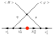
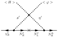
Figure 1: Neutrino mass in the gauge basis at the two-loop level, where the right plot represents the red dot in the left plot.

where $i,a,b=1,2,3$ are the flavor indices for the SM and exotic fermions, and $\tilde{\eta}\equiv i\sigma_{2}\eta^{*}$, with $\sigma_{2}$ being the second Pauli matrix. For simplicity, we assume that all coefficients are real and $M_{\chi},M_{N},M_{N^{\prime}}$ to be diagonal matrices. The first term of $\mathcal{L}_{Y}$ generates the SM charged-lepton masses $m_{\ell_{i}}\equiv y_{\ell_{i}}v_{H}/\sqrt{2}$, while the $2$nd to $4$th terms will be responsible for the (semi-)annihilations. The residual $\mathbb{Z}_{3}$ from the broken hidden symmetry makes the lightest neutral states with $U(1)_{H}$ charge of $x$ or $\pm 2x$, i.e. particles in the set of $(\chi_{i},N^{\prime}_{i},\eta,s)$, to be our DM candidate. While in this paper we are interested in the mass pattern where $\chi_{1}$ actually plays the role of DM. Referring to Table 1, we can see that the two scalar fields $(\Delta,\varphi)$ carrying a $U(1)_{H}$ charge $q_{H}=-3x$ with $x\in$ integer, so that they will transform under the Abelian $U(1)$ symmetry as $\Delta\to e^{-iq_{H}\alpha}\Delta$ and $\varphi\to e^{-iq_{H}\alpha}\varphi$, for an arbitrary value of $\alpha$ before the spontaneous symmetry breaking. However after these two scalars obtain VEVs, the phase is forced to be $\alpha=2\pi/3$ for any integer $x\geq 1$, thus the Lagrangian is still invariant under a discrete $\mathbb{Z}_{3}$ symmetry. And the particles with $x(2x)$ charge in $U(1)_{H}$ have $w=e^{i2\pi/3}(w^{2})$ parity assignment under this $\mathbb{Z}_{3}$.

II.1 The scalar potential

We explicitly write the nontrivial terms for the inert scalar potential which are invariant under the $SU(2)_{L}\times U(1)_{Y}\times U(1)_{H}$ gauge symmetry to be:

$$\mathcal{V}_{1} =\left(\lambda_{0}H^{\dagger}\eta s^{*}\varphi+{\lambda^{\prime}_{0}H^{\dagger}\eta^{\prime}s^{\prime*}\varphi^{*}}+{\rm h.c.}\right)+\sum_{\phi}^{\eta,\eta^{\prime},s,s^{\prime}}\left[\lambda_{H\phi}(H^{\dagger}H)(\phi^{\dagger}\phi)+\lambda_{\varphi\phi}(\varphi^{\dagger}\varphi)(\phi^{\dagger}\phi)\right]$$

$$+\sum_{\phi}^{\eta,\eta^{\prime}}\lambda^{\prime}_{H\phi}(H^{\dagger}\phi)(\phi^{\dagger}H)+\sum_{\phi}^{\eta,\eta^{\prime},s,s^{\prime}}\left[\mu^{2}_{\phi}\phi^{\dagger}\phi+\lambda_{\phi}|\phi^{\dagger}\phi|^{2}\right]\,.$$ (II.2)

where we assume that these terms like $s^{\prime 2}\varphi^{(*)}$, $s^{\prime 2}\varphi^{2}$, $\eta^{\prime{\dagger}}\eta\varphi^{2}$ vanish due to $U(1)_{H}$ charges (e.g. $x=y=1$). Thus no mass splitting occurs among the real and imaginary parts of any inert field. The general potential for the scalars $(H,\Delta)$ can be found in ref Bonilla:2015eha ; Primulando:2019evb , and we will modify it by adding interactions with a complex singlet $\varphi$.

$$\mathcal{V}_{2} = -\mu_{H}^{2}H^{\dagger}H+\lambda_{H}(H^{\dagger}H)^{2}+M^{2}Tr(\Delta^{\dagger}\Delta)+\lambda_{1}(Tr(\Delta^{\dagger}\Delta))^{2}$$ (II.3)

$$+ \lambda_{2}Tr((\Delta^{\dagger}\Delta)^{2})+\lambda_{3}(H^{\dagger}H)Tr(\Delta^{\dagger}\Delta)+\lambda_{4}H^{\dagger}\Delta\Delta^{\dagger}H$$

$$- \mu_{\varphi}^{2}\varphi^{*}\varphi+\lambda_{\varphi}(\varphi^{*}\varphi)^{2}+\lambda_{5}H^{\dagger}H\varphi^{*}\varphi+\lambda_{6}Tr(\Delta^{\dagger}\Delta)\varphi^{*}\varphi$$

$$+ \left[\lambda_{\Delta}H^{T}i\sigma_{2}\Delta^{+}H\varphi+{\rm h.c.}\right]$$

The scalar fields beside the inert ones are explicitly expressed as:

$$H=\left[\begin{array}[]{c}G^{+}\\ \frac{v_{H}+h+iG^{0}}{\sqrt{2}}\end{array}\right]\,,\quad\Delta=\left[\begin{array}[]{cc}\frac{\Delta^{+}}{\sqrt{2}}&\Delta^{++}\\ \frac{v_{\Delta}+\Delta_{R}+i\Delta_{I}}{\sqrt{2}}&-\frac{\Delta^{+}}{\sqrt{2}}\end{array}\right]\,,\quad\varphi=\frac{v_{\varphi}+\varphi_{R}+i\varphi_{I}}{\sqrt{2}}\,.$$ (II.8)

so that the mass of $W$ boson is fixed to be $m_{W}=\frac{g_{2}\sqrt{v_{H}^{2}+2v_{\Delta}^{2}}}{2}$. The minimum of the potential is determined by derivatives $\partial\mathcal{V}_{2}/\partial v_{H}=0$, $\partial\mathcal{V}_{2}/\partial v_{\Delta}=0$, $\partial\mathcal{V}_{2}/\partial v_{\varphi}=0$, which read as:

$$-\mu_{H}^{2}+\lambda_{H}v_{H}^{2}+\frac{\lambda_{3}+\lambda_{4}}{2}v_{\Delta}^{2}+\frac{\lambda_{5}}{2}v_{\varphi}^{2}=\lambda_{\Delta}v_{\Delta}v_{\varphi}$$

$$(M^{2}+\frac{\lambda_{3}+\lambda_{4}}{2}v_{H}^{2}+(\lambda_{1}+\lambda_{2})v_{\Delta}^{2}+\frac{\lambda_{6}}{2}v_{\varphi}^{2})v_{\Delta}=\lambda_{\Delta}v_{H}^{2}v_{\varphi}/2$$

$$(-\mu_{\varphi}^{2}+\lambda_{\varphi}v_{\varphi}^{2}+\frac{\lambda_{5}}{2}v_{H}^{2}++\frac{\lambda_{6}}{2}v_{\Delta}^{2})v_{\varphi}=\lambda_{\Delta}v_{H}^{2}v_{\Delta}/2$$ (II.9)

As we argue in the section [II.4] for $Z-Z^{\prime}$ mixing, $v_{\Delta}$ is very tiny due to the $\rho$ parameter, thus we will focus on the limit of $v_{\Delta}\ll v_{H}\lesssim v_{\varphi}$. Thus under the assumption of negligible mixing between $\varphi$ and $(H,\Delta)$, i.e. $\lambda_{5},\lambda_{6}\ll 1$, we obtain:

$$v_{H}\simeq\left(\frac{\lambda_{\Delta}v_{\Delta}v_{\varphi}+\mu_{H}^{2}}{\lambda_{H}}\right)^{1/2}\,,\quad v_{\Delta}\simeq\frac{\lambda_{\Delta}v_{H}^{2}v_{\varphi}}{2(M^{2}+(\lambda_{3}+\lambda_{4})v_{H}^{2}/2)}\,,\quad v_{\varphi}\simeq\frac{\mu_{\varphi}}{\lambda_{\varphi}^{1/2}}\,.$$ (II.10)

In addition the mass matrices in terms of $(h,\Delta_{R},\varphi_{R})$, $(G^{0},\Delta_{I},\varphi_{I})$ and $(G^{+},\Delta^{+})$ can be diagonalised into CP-even or odd spectrum by respective orthogonal matrices. Analogously the inert bosons $(s,\eta)_{R/I}$ and $(s^{\prime},\eta^{\prime})_{R/I}$ are written as:

$$\eta=\left[\begin{array}[]{c}\eta^{+}\\ \frac{\eta_{R}+i\eta_{I}}{\sqrt{2}}\end{array}\right]\,,\quad s=\frac{s_{R}+is_{I}}{\sqrt{2}}\,;\quad\eta^{\prime}=\left[\begin{array}[]{c}\eta^{\prime+}\\ \frac{\eta^{\prime}_{R}+i\eta^{\prime}_{I}}{\sqrt{2}}\end{array}\right]\,,\quad s^{\prime}=\frac{s^{\prime}_{R}+is^{\prime}_{I}}{\sqrt{2}}\,.$$ (II.15)

They are rotated into the mass basis as follows:

$$V_{\alpha}^{T}\left[\begin{array}[]{cc}m_{s_{R}}^{2}&\frac{\lambda_{0}}{2}v_{H}v_{\varphi}\\ \frac{\lambda_{0}}{2}v_{H}v_{\varphi}&m_{\eta_{R}}^{2}\\ \end{array}\right]V_{\alpha}=\left[\begin{array}[]{cc}m^{2}_{H_{1}}&0\\ 0&m^{2}_{H_{2}}\end{array}\right],~{}~{}V_{\alpha^{\prime}}^{T}\left[\begin{array}[]{cc}m_{s^{\prime}_{R}}^{2}&\frac{\lambda^{\prime}_{0}}{2}v_{H}v_{\varphi}\\ \frac{\lambda^{\prime}_{0}}{2}v_{H}v_{\varphi}&m_{\eta^{\prime}_{R}}^{2}\\ \end{array}\right]V_{\alpha^{\prime}}=\left[\begin{array}[]{cc}m^{2}_{H^{\prime}_{1}}&0\\ 0&m^{2}_{H^{\prime}_{2}}\end{array}\right]$$ (II.24)

$$\left[\begin{array}[]{c}s_{R}+is_{I}\\ \eta_{R}+i\eta_{I}\end{array}\right]=\left[\begin{array}[]{cc}c_{\alpha}&-s_{\alpha}\\ s_{\alpha}&c_{\alpha}\end{array}\right]\left[\begin{array}[]{c}H_{1}+iA_{1}\\ H_{2}+iA_{2}\end{array}\right],\quad\left[\begin{array}[]{c}s^{\prime}_{R}+is^{\prime}_{I}\\ \eta^{\prime}_{R}+i\eta^{\prime}_{I}\end{array}\right]=\left[\begin{array}[]{cc}c_{\alpha^{\prime}}&-s_{\alpha^{\prime}}\\ s_{\alpha^{\prime}}&c_{\alpha^{\prime}}\end{array}\right]\left[\begin{array}[]{c}H^{\prime}_{1}+iA^{\prime}_{1}\\ H^{\prime}_{2}+iA^{\prime}_{2}\end{array}\right]$$ (II.37)

where we use shorthands of $s_{\alpha^{(^{\prime})}}=\sin\alpha^{(^{\prime})}$, $c_{\alpha^{(^{\prime})}}=\cos\alpha^{(^{\prime})}$ and the complex fields $H_{i}+iA_{i}$, $H^{\prime}_{i}+iA^{\prime}_{i}$, $i=1,2$ are mass eigenstates. Note that the semi-annihilation exists for the theory with a $\mathbb{Z}_{3}$ parity, indicating that we need to keep the degeneracy between $H_{1,(2)}$ and $A_{1,(2)}$. The reason is that a $\mathbb{Z}_{3}$ parity assignment $w=e^{i2\pi/3}$ is valid for a Dirac fermion or a complex scalar field, like $\tilde{H}_{i}=H_{i}+iA_{i}$ with $i=1,2$. Under this specific potential we obtain that: $m^{2}_{H_{1,2}}=m^{2}_{A_{1,2}}$, $m^{2}_{H^{\prime}_{1,2}}=m^{2}_{A^{\prime}_{1,2}}$. Without loss of generality, we can assume $m_{H_{1}}<m_{H_{2}}$ and $m_{H^{\prime}_{1}}<m_{H^{\prime}_{2}}$ by ordering the mass eigenstates.

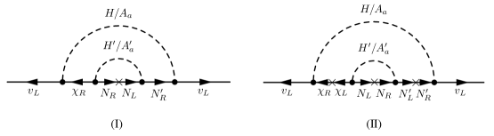
Figure 2: The Feynman diagrams for neutrino masses generated at the two-loop level in the mass eigenstate basis of inert scalars.

II.2 Neutrino mass matrix

In this model, the neutrino mass arises at the 2-loop level. To facilitate the calculation, the Lagrangian should be transformed into the mass basis:

$$-\mathcal{L}_{Y} \sim\frac{y_{\eta_{ia}}}{\sqrt{2}}\bar{\nu}_{L_{i}}\chi_{R_{a}}(s_{\alpha}H_{1}+c_{\alpha}H_{2})-i\frac{y_{\eta_{ia}}}{\sqrt{2}}\bar{\nu}_{L_{i}}\chi_{R_{a}}(s_{\alpha}A_{1}+c_{\alpha}A_{2})$$

$$+\frac{y_{\chi_{ab}}^{L/R}}{\sqrt{2}}\bar{\chi}_{L_{a}/R_{a}}^{C}\chi_{L_{a}/R_{b}}(c_{\alpha}H_{1}-s_{\alpha}H_{2})+i\frac{y_{\chi_{ab}}^{L/R}}{\sqrt{2}}\bar{\chi}_{L_{a}/R_{a}}^{C}\chi_{L_{a}/R_{b}}(c_{\alpha}A_{1}-s_{\alpha}A_{2})$$

$$+\frac{y_{S_{ia}}}{\sqrt{2}}\bar{\nu}_{L_{i}}N^{\prime}_{R_{a}}(c_{\alpha}H_{1}-s_{\alpha}H_{2})+i\frac{y_{S_{ia}}}{\sqrt{2}}\bar{\nu}_{L_{i}}N^{\prime}_{R_{a}}(c_{\alpha}A_{1}-s_{\alpha}A_{2})$$

$$+\frac{y_{s^{\prime}_{ab}}}{\sqrt{2}}\bar{N}_{R_{a}}\chi^{C}_{R_{b}}(c_{\alpha^{\prime}}H^{\prime}_{1}-s_{\alpha^{\prime}}H^{\prime}_{2})+i\frac{y_{s^{\prime}_{ab}}}{\sqrt{2}}\bar{N}_{R_{a}}\chi^{C}_{R_{b}}(c_{\alpha^{\prime}}A^{\prime}_{1}-s_{\alpha^{\prime}}A^{\prime}_{2})$$

$$+\frac{y^{\prime}_{s^{\prime}_{ab}}}{\sqrt{2}}\bar{N}_{L_{a}}\chi^{C}_{L_{b}}(c_{\alpha^{\prime}}H^{\prime}_{1}-s_{\alpha^{\prime}}H^{\prime}_{2})+i\frac{y^{\prime}_{s^{\prime}_{ab}}}{\sqrt{2}}\bar{N}_{L_{a}}\chi^{C}_{L_{b}}(c_{\alpha^{\prime}}A^{\prime}_{1}-s_{\alpha^{\prime}}A^{\prime}_{2})$$

$$+\frac{y_{\eta^{\prime}_{ab}}}{\sqrt{2}}\bar{N}^{\prime}_{R_{a}}N_{L_{b}}(s_{\alpha^{\prime}}H^{\prime}_{1}+c_{\alpha^{\prime}}H^{\prime}_{2})-i\frac{y_{\eta^{\prime}_{ab}}}{\sqrt{2}}\bar{N}^{\prime}_{R_{a}}N_{L_{b}}(s_{\alpha^{\prime}}A^{\prime}_{1}+c_{\alpha^{\prime}}A^{\prime}_{2})$$

$$+\frac{y^{\prime}_{\eta^{\prime}_{ab}}}{\sqrt{2}}\bar{N}^{\prime}_{L_{a}}N_{R_{b}}(s_{\alpha^{\prime}}H^{\prime}_{1}+c_{\alpha^{\prime}}H^{\prime}_{2})-i\frac{y^{\prime}_{\eta^{\prime}_{ab}}}{\sqrt{2}}\bar{N}^{\prime}_{L_{a}}N_{R_{b}}(s_{\alpha^{\prime}}A^{\prime}_{1}+c_{\alpha^{\prime}}A^{\prime}_{2})+{\rm h.c.}.$$ (II.38)

Here we assume that all the Yukawa couplings are real for simplicity. The active neutrino mass matrix $m_{\nu_{ij}}$ are generated at two-loop level as shown in Figure 2, with their formulas given by

$$(m_{\nu})_{ij}=m_{\nu_{ij}}^{(I)}+m_{\nu_{ij}}^{(II)}+[m_{\nu_{ij}}^{(I)}]^{T}+[m_{\nu_{ij}}^{(II)}]^{T},$$ (II.39)

where $m_{\nu_{ab}}^{(I)}$ and $m_{\nu_{ab}}^{(II)}$ respectively correspond to the left and right plots in Figure 2. The constraint on the neutrino matrix is from the neutrino oscillation data, since $({m}_{\nu})_{ab}$ have to be diagonalized by the Pontecorvo-Maki-Nakagawa-Sakata mixing matrix $V_{\rm MNS}$ (PMNS) Maki:1962mu as $({m}_{\nu})_{ij}=(V_{\rm MNS}^{*}D_{\nu}V_{\rm MNS}^{\dagger})_{ij}$ with $D_{\nu}=\rm{diag}(m_{\nu_{1}},m_{\nu_{2}},m_{\nu_{3}})$. The PMNS matrix is parametrised as:

$$V_{\rm MNS} =\left[\begin{array}[]{ccc}{c_{13}}c_{12}&c_{13}s_{12}&s_{13}e^{-i\delta}\\ -c_{23}s_{12}-s_{23}s_{13}c_{12}e^{i\delta}&c_{23}c_{12}-s_{23}s_{13}s_{12}e^{i\delta}&s_{23}c_{13}\\ s_{23}s_{12}-c_{23}s_{13}c_{12}e^{i\delta}&-s_{23}c_{12}-c_{23}s_{13}s_{12}e^{i\delta}&c_{23}c_{13}\\ \end{array}\right]$$ (II.43)

$$\times\rm{diag}(1,e^{i\frac{\alpha_{21}}{2}},e^{i\frac{\alpha_{31}}{2}})$$ (II.44)

with $s_{ij}=\sin\theta_{ij}$ being three mixing angles. In the following analysis, we will also neglect the Majorana CP violation phase $\alpha_{21}$ and $\alpha_{31}$ as well as Dirac CP violation phase $\delta$. By assuming the normal mass order $m_{\nu 1}\ll m_{\nu 2}<m_{\nu 3}$, the global fit of the current experiments at $3\sigma$ is given by pdg2018 :

$$0.250\leq s_{12}^{2}\leq 0.354,\;0.381\leq s_{23}^{2}\leq 0.615,\;0.019\leq s_{13}^{2}\leq 0.024,$$

$$m_{\nu_{3}}^{2}-m_{\nu_{1}}^{2}=(2.45-2.69)\times 10^{-3}\ {\rm eV}^{2},$$

$$\ m_{\nu_{2}}^{2}-m_{\nu_{1}}^{2}=(6.93-7.96)\times 10^{-5}\ {\rm eV}^{2},$$ (II.45)

Now we rewrite the neutrino mass matrix in terms of Yukawa couplings and the form factors:

$$(m_{\nu})_{ij}\equiv\frac{1}{(4\pi)^{4}}\left(y_{\eta_{ia}}[F_{I}+F_{II}]_{ab}y^{T}_{S_{bj}}+y_{S_{ja}}[F_{I}^{T}+F_{II}^{T}]_{ab}y^{T}_{\eta_{bj}}\right)$$

$$\equiv\frac{1}{(4\pi)^{4}}\left(y_{\eta_{ia}}G_{ab}y^{T}_{S_{bj}}+y_{S_{ja}}G^{T}_{ab}y^{T}_{\eta_{bj}}\right),$$ (II.46)

where the factor $\frac{1}{(4\pi)^{4}}$ comes from the loop integration and the exact expressions for these form factors $F_{I}$, $F_{II}$ are put in Appendix A. The form factors exhibit an interesting property, proportional to the product of mass differences $(m_{H_{2}}^{2}-m_{H_{1}}^{2})(m_{H^{\prime}_{2}}^{2}-m_{H^{\prime}_{1}}^{2})$. Thus the neutrino mass can be easily accommodated into the sub-eV order, if either one set of inert scalars is quasi-degenerate without tuning the Yukawa couplings. In particular, if we set $m_{H^{\prime}_{1}}\simeq m_{H^{\prime}_{2}}$, the LFV bound will not be influenced as $H^{\prime}_{1,2}$ do not mediate these processes.

Due to the symmetric property, the Eq. (II.46) can be conveniently recasted into a suitable form for the numerical analysis:

$$y_{\eta}=\frac{1}{2}[(V_{\rm MNS}^{*}D_{\nu}V_{\rm MNS}^{\dagger}+A](y^{T}_{S})^{-1}G^{-1},$$ (II.47)

where the $A$ is an arbitrary anti-symmetric matrix in the order $\lesssim 10^{-9}$ and of complex values if there is CP violation Okada:2015vwh . Therefore after we impose Eq.(II.47), the $y_{\eta}$ coupling is no longer a free parameter but as a function of $y_{S}$ and the neutrino mass form factors. This parameter will be determined by the neutrino oscillation data up to an uncertainty. Notice that $y_{\eta}\lesssim\sqrt{4\pi}$ should be satisfied in the perturbative limit.

II.3 LFV and Muon $g-2$

In this radiative neutrino mass model, the existence of charged scalars and vector-like fermions contribute to lepton flavor violation processes (see Figure. 3), which in turn will severely constrain the Yukawa couplings and masses of heavy scalars and fermions. The relevant Lagrangian for LFV can be expressed as:

$${\cal L}={-}y_{\eta_{ia}}\bar{\ell}_{L_{i}}\eta^{-}\chi_{R_{a}}+\frac{1}{\sqrt{2}}y_{S_{ia}}\bar{\ell}_{L_{i}}E^{\prime}_{R_{a}}[(c_{\alpha_{R}}H_{1}-s_{\alpha_{R}}H_{2})+i(c_{\alpha_{I}}A_{1}-s_{\alpha_{I}}A_{2})]+{\rm h.c.},$$ (II.48)

We can calculate the branching ratio for LFV decay process $\ell_{i}\to\ell_{j}\gamma$ in terms of amplitude $a_{L/R}$, which encodes the loop integration of the Feynman diagrams:

$$Br(\ell_{i}\to\ell_{j}\gamma)\approx\frac{48\pi^{3}\alpha_{\rm em}}{{G_{\rm F}^{2}m_{\ell_{i}}^{2}}}C_{ij}\left(|a_{L_{ij}}|^{2}+|a_{R_{ij}}|^{2}\right),$$ (II.49)

where $G_{\rm F}\approx 1.166\times 10^{-5}$ GeV^-2 is the Fermi constant, $\alpha_{\rm em}(m_{Z})\approx{1/128.9}$ is the fine-structure constant pdg2018 , $C_{21}\approx 1$, $C_{31}\approx 0.1784$, and $C_{32}\approx 0.1736$. In this specific model $a_{R}$ is formulated as:

$$a_{R_{ij}}\approx\frac{m_{\ell_{i}}}{(4\pi)^{2}}\left[y_{\eta_{ja}}y^{\dagger}_{\eta_{ai}}H(\chi_{a},\eta^{-})\right.$$

$$\left.-\frac{y_{S_{ja}}y^{\dagger}_{S_{ai}}}{2}[c^{2}_{\alpha_{R}}H(H_{1},E^{\prime}_{a})+s^{2}_{\alpha_{R}}H(H_{2},E^{\prime}_{a})+c^{2}_{\alpha_{I}}H(A_{1},E^{\prime}_{a})+s^{2}_{\alpha_{I}}H(A_{2},E^{\prime}_{a})]\right],$$ (II.50)

$$H(a,b)=\int_{0}^{1}dx\int_{0}^{1-x}dy\frac{xy}{x~{}m^{2}_{a}+(1-x)~{}m^{2}_{b}}$$

$$\quad\quad\overset{m_{a}\neq m_{b}}{=}\frac{2m_{a}^{6}+3m_{a}^{4}m_{b}^{2}-6m_{a}^{2}m_{b}^{4}+m_{b}^{6}+6m_{a}^{4}m_{b}^{2}\log\left(\frac{m_{b}^{2}}{m_{a}^{2}}\right)}{12\left(m_{a}^{2}-m_{b}^{2}\right)^{4}}$$ (II.51)

where we can see that the loop contributions from two resources (Figure 2.a and Figure 2.b) are in opposite signs. And for the left-handed amplitude, $a_{L}$ is obtained by a mass substitution: $a_{L}=a_{R}(m_{\ell_{i}}\to m_{\ell_{j}})$.

The couplings involved in those LFV processes are $y_{\eta}$ and $y_{S}$, strongly correlated to the neutrino mass matrix. In particular the magnitude of $y_{\eta}$ along with masses $m_{\chi_{1}}$ and $m_{H_{1,2}}$, constrained by the LFV bound, will influence the DM relic density as well. To find out the allowed parameter space for this model, the following upper bounds are imposed TheMEG:2016wtm ; Aubert:2009ag

$$\quad\quad\quad Br(\mu\rightarrow e\gamma)\leq 4.2\times 10^{-13}~{}(6\times 10^{-14})$$

$$Br(\tau\rightarrow\mu\gamma)\leq 4.4\times 10^{-8},\quad Br(\tau\rightarrow e\gamma)\leq 3.3\times 10^{-8}$$ (II.52)

where the upper bound from $\mu\to e\gamma$ is the most stringent one with the value in parentheses indicating a future reach of MEG experiment Renga:2018fpd .

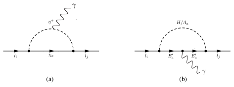
Figure 3: Lepton flavor violation processes induced by heavy fermions and scalars.

The muon anomalous magnetic moment: The muon $g-2$ is a well-measured property and a large $3.6\sigma$ discrepancy of $\Delta a_{\mu}$ between the SM theory and experiment measurement was observed for a long time. For this model, one can estimate the muon $g-2$ through the amplitudes formulated above:

$$\Delta a_{\mu}\approx-m_{\mu}(a_{L}+a_{R})_{22}.$$ (II.53)

The deviation from the SM prediction is $\Delta a_{\mu}=a_{\mu}^{\rm exp}-a_{\mu}^{\rm SM}=(2.74\pm 0.73)\times 10^{-9}$ pdg2018 with a positive value. However because our analysis shows the muon $g-2$ is too tiny after imposing other bounds, we just employ the muon $g-2$ as a model quality for reference.

II.4 $Z-Z^{\prime}$ mixing

The effect of the hidden $Z^{\prime}$ at TeV scale will actually decouple from the dark matter physics and we would like to qualify this argument in the section. After the three scalar fields developing VEVs, $U(1)_{H}$ and electroweak symmetries are spontaneously broken so that the mass terms of neutral gauge boson are obtained,

$$\frac{1}{2}\begin{pmatrix}Z_{0}\\ \tilde{Z}\end{pmatrix}^{T}\left[\begin{array}[]{cc}\frac{(g_{1}^{2}+g_{2}^{2})}{4}(v_{H}^{2}+4v_{\Delta}^{2})&3x\sqrt{g_{1}^{2}+g_{2}^{2}}g_{H}v_{\Delta}^{2}\\ 3x\sqrt{g_{1}^{2}+g_{2}^{2}}g_{H}v_{\Delta}^{2}&9x^{2}g_{H}^{2}(v_{\Delta}^{2}+v_{\varphi}^{2})\\ \end{array}\right]\begin{pmatrix}Z_{0}\\ \tilde{Z}\end{pmatrix},$$ (II.56)

where $g_{2}$, $g_{1}$ and $g_{H}$ are gauge couplings of $SU(2)_{L}$, $U(1)_{Y}$, and $U(1)_{H}$, respectively. The $Z_{0}$ and $\tilde{Z}$ are the gauge fields for $U(1)_{Y}$ and $U(1)_{H}$ with the $Z_{0}$ mostly composed of the SM Z boson. Here we assume the kinetic mixing between the two Abelian gauge bosons to be negligibly small for simplicity. In case of $x=1$, we parameterise the mass matrix to be:

$$\left[\begin{array}[]{cc}\frac{(g_{1}^{2}+g_{2}^{2})}{4}(v_{H}^{2}+4v_{\Delta}^{2})&3~{}\sqrt{g_{1}^{2}+g_{2}^{2}}g_{H}v_{\Delta}^{2}\\ 3~{}\sqrt{g_{1}^{2}+g_{2}^{2}}g_{H}v_{\Delta}^{2}&9~{}g_{H}^{2}(v_{\Delta}^{2}+v_{\varphi}^{2})\\ \end{array}\right]=m_{\tilde{Z}}^{2}\left[\begin{array}[]{cc}\epsilon_{1}^{2}&2\epsilon_{1}\epsilon_{2}\epsilon_{3}\\ 2\epsilon_{1}\epsilon_{2}\epsilon_{3}&1+\epsilon_{2}^{2}\\ \end{array}\right],$$ (II.57)

where we use the definition of $m_{Z_{0}}=\frac{\sqrt{(g_{1}^{2}+g_{2}^{2})\left(v_{H}^{2}+4v_{\Delta}^{2}\right)}}{2}$, $m_{\tilde{Z}}=3g_{H}v_{\varphi}$, $\epsilon_{1}=\frac{m_{Z_{0}}}{m_{\tilde{Z}}}$ and $\epsilon_{2}=\frac{v_{\Delta}}{v_{\varphi}}$, $\epsilon_{3}=\frac{v_{\Delta}}{\sqrt{v_{H}^{2}+4v_{\Delta}^{2}}}$. The mass matrix can be diagonalized by an orthogonal transformation to be ${\rm Diag}(m^{2}_{Z},m^{2}_{Z^{\prime}})$, and in an approximation of $v_{\Delta}\ll v_{H}\lesssim v_{\varphi}$ and $g_{H}=\mathcal{O}(1)$, this gives:

$$m^{2}_{Z} \approx m_{Z_{0}}^{2}\left(1-4\epsilon_{2}^{2}\epsilon_{3}^{2}\right),\,\quad m^{2}_{Z^{\prime}}\approx m_{\tilde{Z}}^{2}\left(1+\epsilon_{2}^{2}\right),$$ (II.58)

$$\begin{pmatrix}Z\\ Z^{\prime}\end{pmatrix} =\left[\begin{array}[]{cc}c_{Z}&s_{Z}\\ -s_{Z}&c_{Z}\\ \end{array}\right]\begin{pmatrix}Z_{0}\\ \tilde{Z}\end{pmatrix},\quad\tan\theta_{Z}=\frac{-2\epsilon_{1}\epsilon_{2}\epsilon_{3}}{1+\epsilon_{2}^{2}-\epsilon_{1}^{2}}.$$ (II.61)

If we fix $c_{W}^{2}=g_{2}^{2}/(g_{1}^{2}+g_{2}^{2})$ as the SM value, the $\rho$ parameter can be expressed to be:

$$\rho_{0}\simeq\frac{\left(1+\frac{2v_{\Delta}^{2}}{v_{H}^{2}}\right)}{\left(1+\frac{4v_{\Delta}^{2}}{v_{H}^{2}}\right)\left(1-4\epsilon_{2}^{2}\epsilon_{3}^{2}\right)}$$ (II.62)

The experimental constraint from the PDG is $\rho_{0,\,\rm{exp}}=1.00039\pm 0.00019$ pdg2018 , which will translate into a requirement of $v_{\Delta}\lesssim 3.5$ GeV. In this paper, we assume the $Z^{\prime}$ boson mass to be above the TeV scale for $v_{\varphi}\gtrsim 350$ GeV. According to Eq. (II.61), this results in a extremely small $|\tan\theta_{Z}|<10^{-5}$ compared with the Yukawa coupling with DM and neutrino. Thus as long as we prefer the DM mass in $\mathcal{O}(100)$ GeV, it will be safe to neglect the the impact of $Z^{\prime}$ on either DM annihilation or DM-nucleon scattering,

II.5 Bound of Electroweak Precision Test

The Electroweak Precision Test (EWPT) on low energy observables can set limits for deviations from the SM. The new physics effects are mainly encoded the oblique parameters $S$, $T$ and $U$, expressed in terms of the transverse part of gauge boson’s self-energy amplitudes. For this model, since the $U$ parameter is suppressed by an additional factor of $v^{2}/M_{\mbox{new}}^{2}$, its effect is neglected. Due to the vector-like nature and degeneracy, the exotic particles of $L^{\prime}_{i}$ have no impact on oblique parameters, i.e. $\Delta S_{f}=\frac{2}{3\pi}(t_{3L}-t_{3R})^{2}=0$ and $\Delta T_{f}=0$ pdg2018 . However the inert scalars $(\eta,s)$ are possible to cause notable deviation to $S=-16\pi\Pi^{\prime}(0)_{W_{3}B}$ and $T=\frac{4\pi}{m_{Z}^{2}s^{2}_{W}c^{2}_{W}}\left[2\Pi_{W_{1}W_{1}}(0)-\Pi_{W_{3}W_{3}}(0)\right]$ Peskin:1991sw , we will discuss their constraints on the mass splitting among $(m_{\eta^{+}},m_{H_{i}})$ and the mixing angle $\sin(\alpha)$. After evaluating the relevant self-energy correlations, we find out the effects from the inert scalars are described by:

$$\Delta S = \frac{1}{12\pi}\left[s_{\alpha}^{4}G(m_{H_{1}},m_{H_{1}},m_{\eta^{+}})+c_{\alpha}^{4}G(m_{H_{2}}m_{H_{2}},m_{\eta^{+}})+2c_{\alpha}^{2}s_{\alpha}^{2}G(m_{H_{1}},m_{H_{2}},m_{\eta^{+}})\right]$$ (II.63)

$$= \frac{1}{12\pi}\left[s_{\alpha}^{2}\ln\left(\frac{m_{H_{1}}^{2}}{m_{\eta^{+}}^{2}}\right)+c_{\alpha}^{2}\ln\left(\frac{m_{H_{2}}^{2}}{m_{\eta^{+}}^{2}}\right)-3c_{\alpha}^{2}s_{\alpha}^{2}\chi(m_{H_{1}},m_{H_{2}})\right]$$

$$\Delta T = \frac{1}{16\pi m_{W}^{2}s_{W}^{2}}[s_{\alpha}^{2}F(m_{H_{1}},m_{\eta^{+}})+c_{\alpha}^{2}F(m_{H_{2}}m_{\eta^{+}})-c_{\alpha}^{2}s_{\alpha}^{2}F(m_{H_{1}},m_{H_{2}})]$$ (II.64)

where the loop functions $G(m_{1},m_{2},m_{3})$, $\chi(m_{1},m_{2})$ and $F(m_{1},m_{2})$ are defined as:

$$G(m_{1},m_{2},m_{3})=\frac{1}{2}\left[\ln\left(\frac{m_{1}^{2}m_{2}^{2}}{m_{3}^{4}}\right)-3\chi(m_{1},m_{2})\right]$$ (II.65)

$$\chi(m_{1},m_{2})=\frac{5\left(m_{1}^{4}+m_{2}^{4}\right)-22m_{1}^{2}m_{2}^{2}}{9\left(m_{1}^{2}-m_{2}^{2}\right)^{2}}+\frac{3m_{1}^{2}m_{2}^{2}\left(m_{1}^{2}+m_{2}^{2}\right)-m_{1}^{6}-m_{2}^{6}}{3\left(m_{1}^{2}-m_{2}^{2}\right)^{3}}\ln\left(\frac{m_{1}^{2}}{m_{2}^{2}}\right)$$ (II.66)

$$F(m_{1},m_{2})=m_{1}^{2}+m_{2}^{2}-\frac{2m_{1}^{2}m_{2}^{2}}{m_{1}^{2}-m_{2}^{2}}\ln\left(\frac{m_{1}^{2}}{m_{2}^{2}}\right).$$ (II.67)

with $\chi(m_{1},m_{2})$ and $F(m_{1},m_{2})$ being symmetric for $m_{1}\leftrightarrow m_{2}$ and vanishing for equal masses, i.e. $\chi(m,m)=F(m,m)=0$. During the calculation, the divergences inherent in the two-point functions are properly cancelled . In case of the SM Higgs $h$ barely mixing with $(\Delta,\varphi)$, the $\Delta T$ is exactly the wave-function renormalisation of the goldstone bosons $G^{+},G^{0}$ with $(\eta^{\pm},((\eta_{R}+i\eta_{I})/\sqrt{2}),s)$ running inside the loops(referring to Appendix B for detail)  Barbieri:2006dq . While for the $\Delta S$, the function $G(m_{1},m_{2},m_{3})$ is related to $\frac{d}{dp^{2}}\left[B_{22}(p^{2},m_{1}^{2},m_{2}^{2})-B_{22}(p^{2},m_{3}^{2},m_{3}^{2})\right]|_{p^{2}=0}=\frac{1}{2}\int_{0}^{1}dx~{}x(1-x)\ln[\frac{xm_{1}^{2}+(1-x)m_{2}^{2}}{m_{3}^{2}}]$, using the Passarino-Veltman function $B_{22}$ defined in Passarino:1978jh .

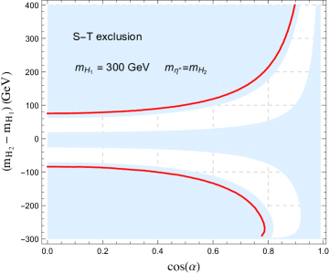
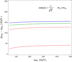
Figure 4: In the left plot, the two white bands present the region allowed by the $S-T$ bound at the $1\sigma$ C.L.; While the red line is the $3\sigma$ bound for $m_{H_{2}}=300$ GeV. The right plot shows the bound for $(m_{H_{2}}-m_{H_{1}})$ and $m_{H_{1}}$ in case of $s_{\alpha}=c_{\alpha}=\frac{1}{\sqrt{2}}$ (assuming $m_{H_{2}}>m_{H_{1}}$ and $m_{\eta^{+}}=m_{H_{2}}$), where the regions outside the contours of red, green and blue lines are excluded at $68\%(1\sigma)$, $95\%(2\sigma)$ and $99\%(3\sigma)$ C.L.s.

The bound for the $S$ and $T$ parameters is obtained from the precision electroweak data, such as $M_{Z}$ and $\Gamma_{Z}$, at the $1\sigma$ deviation by fixing $U=0$ pdg2018 :

$$S=0.02\pm 0.07\qquad T=0.06\pm 0.06$$ (II.68)

with an off-diagonal correlation of $92\%$. In Figure 4, combining all the discussed parts, we translate the $S$-$T$ $\chi^{2}$ fit into the bounds of inert scalar masses and the mixing angle. Since both $\Delta S$ and $\Delta T$ are symmetric functions of $(m_{H_{1}},m_{H_{2}})$, we focus on the case of $m_{\eta^{+}}=m_{H_{2}}$ for simplicity. The operation of switching $H_{1}\leftrightarrow H_{2}$ is to shift the mixing angle by $\alpha\to(\alpha-\frac{\pi}{4})$. the $1\sigma$ EWPT fit prefers the mass splitting $(m_{H_{2}}-m_{H_{1}})>0$ in a small range of $0.92<\cos\alpha<1.0$ , i.e. $H_{2}(A_{2})$ dominantly composed of $\eta_{R}(\eta_{I})$ should be heavier. However at $3\sigma$ fit, $(m_{H_{2}}-m_{H_{1}})$ is permitted in either sign $(+/-)$ for $0<\alpha<\frac{\pi}{2}$, with its magnitude decreasing with $\cos\alpha$. In the right plot, we show that assuming $m_{H_{2}}>m_{H_{1}}$, the $S$-$T$ bound requires $(m_{H_{2}}-m_{H_{1}})\subset(30,120)$ GeV at $1\sigma$ and $(m_{H_{2}}-m_{H_{1}})<150$ GeV at $3\sigma$ for $100<m_{H_{1}}<500$ GeV under the condition specified in the caption.

III Dark matter

The relic density for a DM specie $X$ is determined by its energy density, $\propto m_{X}n_{X}(T_{0})$ in the present universe, where the number density $n_{X}$ is governed by the Boltzmann equation during the decoupling phase plus the afterwards expansion effect. For a Dirac fermion DM stabilised by a $\mathbb{Z}_{3}$ symmetry, semi-annihilation modes in addition to annihilation are expected to contribute. The Boltzmann equation can be recasted into an evolution in terms of a yield by defining $Y_{X}=n_{X}/s$ with $s$ to be entropy density and $x=M_{X}/T$ where the temperature is scaled by the DM mass. The redefined equation reads:

$$\frac{dY_{X}}{dx}=-\frac{\lambda_{\rm A}}{x^{2}}[Y_{X}^{2}-Y_{X}^{\rm{eq}2}]-\frac{1}{2}\frac{\lambda_{\rm S}}{x^{2}}[Y_{X}^{2}-Y_{X}Y_{X}^{\rm{eq}}]\,,$$ (III.1)

$$\lambda_{i}=\frac{s(x=1)}{H(x=1)}\langle\sigma v_{\rm rel}\rangle_{i},\quad i=A,S$$

$$s(x=1)=\frac{2\pi^{2}}{45}g_{*}M_{X}^{3}\,,\quad H(x=1)=\sqrt{\frac{\pi^{2}}{90}g_{*}}\frac{M_{X}^{2}}{M_{\rm pl}}$$ (III.2)

where $A,S$ stand for annihilation and semi-annihilation, $H(x=1)$ is the Hubble constant at $T=M_{X}$, $g_{*}$ is the effective total number of relativistic degrees of freedom and $M_{\rm pl}=1.22\times 10^{19}[{\rm GeV}]$ is the Planck mass. The $\frac{1}{2}$ factor in the second term of Eq. (III.1) is due to the identical initial particles  and $\langle\sigma v_{\rm rel}\rangle$ is the thermal average of velocity weighted cross section which represents the DM interaction rate. This equation can be analytically solved in a proper approximation by matching the results from two regions at the freeze-out point. A brief review for this approach will be presented here in order to clarify the missing $1/2$ in some literature. We will start by defining a quality $\Delta=Y_{X}-Y_{X}^{\rm eq}$, so that the original equation is transformed into:

$$\frac{d\Delta}{dx}=-\frac{dY_{X}^{\rm eq}}{x}-\frac{\lambda_{\rm A}}{x^{2}}[\Delta^{2}+2\Delta Y_{X}^{\rm{eq}}]-\frac{1}{2}\frac{\lambda_{\rm S}}{x^{2}}[\Delta^{2}+\Delta Y_{X}^{\rm{eq}}]$$ (III.3)

where the Maxwell-Boltzmann distribution will be used for the yield in equilibrium so that $Y_{X}^{\rm eq}(x)\propto x^{3/2}e^{-x}$. For $x\ll x_{f}$, we can obtain:

$$\Delta=\frac{Y_{X}^{\rm eq}}{\frac{\lambda_{A}}{x^{2}}(2Y_{X}^{\rm eq}+\Delta)+\frac{\lambda_{S}}{2x^{2}}(Y_{X}^{\rm eq}+\Delta)}$$ (III.4)

and for $x\gg x_{f}$, the integration of Boltzmann equation gives:

$$Y_{X}(\infty)\simeq-\int_{x_{f}}^{\infty}dx\frac{\lambda_{A}+\frac{1}{2}\lambda_{S}}{x^{2}}$$ (III.5)

Thus the relic density at the present universe is found as:

$$\Omega h^{2}=m_{X}s_{0}Y_{X}(\infty)/\rho_{c}\approx 2\frac{1.07\times 10^{9}{\rm GeV}^{-1}}{\sqrt{g_{*}(x_{f})}M_{pl}J(x_{f})},$$ (III.6)

$$J(x_{f})=\int_{x_{f}}^{\infty}dx\frac{\langle\sigma v_{\rm rel}\rangle_{\rm A}+\frac{1}{2}\langle\sigma v_{\rm rel}\rangle_{\rm S}}{x^{2}},$$ (III.7)

where $\Omega h^{2}$ is rescaled by the critical density $\rho_{c}=3H^{2}/8\pi G$. We times a factor $2$ for the relic density in order to count the contribution from the antiparticle $\bar{X}$ and set $g_{*}(x_{f})\approx 100$ at the point of freeze-out. Here $\langle\sigma v\rangle_{\rm A}$ is the thermal average for annihilation, while $\langle\sigma v\rangle_{\rm S}$ is for semi-annihilation. Then the freeze-out temperature $x_{f}$ is determined by the boundary condition $\Delta(x_{f})=c~{}Y_{X}^{\rm eq}(x_{f})$ with $c=\sqrt{2}-1$ to be:

$$x_{f}\simeq\ln\left[0.038c(c+2)\langle\sigma v\rangle_{\rm A}\frac{gM_{X}M_{pl}}{\sqrt{g_{*}x_{f}}}\right]+\ln\left[1+\frac{c+1}{c+2}~{}\frac{\langle\sigma v\rangle_{\rm S}}{2~{}\langle\sigma v\rangle_{\rm A}}\right],$$ (III.8)

which is up to a $1/2$ factor for the semi-annihilation part as given by DEramo:2010keq and we set $g=2$ for a fermion DM of two degrees of freedom without counting its antiparticle Kolb .

As we can see that in order to estimate the relic density, one has to calculate the thermal average of cross section times the relative velocity $\langle\sigma v_{rel}\rangle$. Generally the thermal average is approximated by an expansion in order of $x^{-n}$ ($\langle v^{2}\rangle\sim\frac{6}{x}$ in the non-relativistic limit). However in our case, the dominant DM cross section proceeds through an $S$-channel with one very narrow resonance $\Gamma_{M}/M_{X}\ll v_{\rm rel}$ and one wider resonance $\Gamma_{M}/M_{X}\sim v_{\rm rel}$. Also for a $S$-channel interaction mediated by a scalar, the s-wave is vanishing for the velocity averaged cross section, thus the expansion in terms of $v_{\rm rel}^{2}$ is complicated to handle for two resonances interfering with each other. We prefer to use the integration approach to evaluate $\langle\sigma v_{\rm rel}\rangle$ which is given by Gondolo:1990dk ; Edsjo:1997bg

$$\langle\sigma v_{\rm rel}\rangle_{A}=\sum_{i=1}^{2}\frac{\int_{4M^{2}_{X}}^{\infty}~{}ds~{}\sigma_{XX}^{i}(s-4M_{X}^{2})\sqrt{s}K_{1}\left(\frac{\sqrt{s}}{M_{X}}x\right)}{8M_{X}^{5}x^{-1}K_{2}(x)^{2}}$$ (III.9)

$$\langle\sigma v_{\rm rel}\rangle_{S}=\frac{\int_{4M^{2}_{X}}^{\infty}~{}ds~{}\sigma_{XX}^{3}(s-4M_{X}^{2})\sqrt{s}K_{1}\left(\frac{\sqrt{s}}{M_{X}}x\right)}{8M_{X}^{5}x^{-1}K_{2}(x)^{2}}$$ (III.10)

where $s=(k_{1}+k_{2})^{2}$ is a Mandelstam variable and $K_{1,2}$ are the modified Bessel functions of order 1 and 2 respectively.

$$\sigma_{XX}^{i}=\frac{|\bf{k}_{1}|}{32\pi^{2}s\sqrt{s-4M_{X}^{2}}}\int d\Omega|\bar{\cal M}_{i}|^{2},i=1,2,3;$$ (III.11)

$$\mbox{\rm with}~{}~{}|{\bf{k}}_{1}|=\sqrt{\frac{s}{4}-m_{l/\nu}^{2}}~{}~{}i=1,2;\quad|{\bf{k}}_{1}|=\frac{s-M_{X}^{2}}{2\sqrt{s}}~{}~{}i=3.$$

Here $\sigma_{XX}^{i}$ is the cross section of the $2\to 2$ process (denoting $\bf{k}_{1}$ as 3-momentum of the first out-going particle) and with the amplitude squared $|{\cal\bar{M}}_{1,2}|^{2}$ corresponding to $X\bar{X}\to\nu_{i}\bar{\nu}_{j}$ and $X\bar{X}\to\ell_{i}\bar{\ell}_{j}$ in Fig. 5(a-b) and the third $|{\cal\bar{M}}_{3}|^{2}$ standing for $XX\to\bar{X}\nu_{i}$, i.e. the semi-annihilation as depicted in Fig. 5(c)-(e).

Figure 5: Feynman diagrams for the annihilation (a)-(b) and semi-annihilation processes (c)-(e), where the mediating scalar fields are $H_{a}$ or $A_{a}$, with $a=1,2$.

We derive the analytic expression for each amplitude squared present in Eq.(III.11). Let us consider the case that only the lightest flavor of $\chi_{i}$ is the DM candidate. By defining $X=\chi_{1}$ and assuming $y^{L}_{\chi}=y^{R}_{\chi}$, the DM-scalar interaction in this model is written as:

$$-{\cal L} =\frac{y_{\eta_{i1}}}{\sqrt{2}}\bar{\nu}_{i}P_{R}X(s_{\alpha}H_{1}+c_{\alpha}H_{2})-i\frac{y_{\eta_{i1}}}{\sqrt{2}}\bar{\nu}_{i}P_{R}X(s_{\alpha}A_{1}+c_{\alpha}A_{2}){-}y_{\eta_{i1}}\bar{\ell}_{i}P_{R}X\eta^{-}$$

$$+\frac{y_{\chi_{11}}}{\sqrt{2}}\bar{X}^{C}X(c_{\alpha}H_{1}-s_{\alpha}H_{2}){+i}\frac{y_{\chi_{11}}}{\sqrt{2}}\bar{X}^{C}X(c_{\alpha}A_{1}-s_{\alpha}A_{2})+{\rm h.c.}\,,$$ (III.12)

For the annihilation processes, $|{\cal\bar{M}}_{1,2}|$ are the usual amplitude squared with the spin averaged for the initial states and summed for the final states. However a special treatment is needed for $|{\cal\bar{M}}_{3}|$ because of the identical incoming particles. As illustrated in Fig. 5(c)-(e), the semi-annihilation proceeds in $S$, $T$ and $U$ channels after counting the momentum exchanging for the identical initial particles. In particular, there is a symmetry factor $2$ for the $S$-channel amplitude . Combining all channels, we can arrive the following analytic expressions:

$$|{\cal\bar{M}}_{1}|^{2} =\sum_{i,j=1}^{3}{|y_{\eta_{i1}}y_{\eta_{1j}}^{\dagger}|^{2}}\left|\frac{s_{\alpha}^{2}}{M_{X}^{2}-m_{H_{1}}^{2}-2p_{1}\cdot k_{1}}+\frac{c_{\alpha}^{2}}{M_{X}^{2}-m_{H_{2}}^{2}-2p_{1}\cdot k_{1}}\right|^{2}(p_{1}\cdot k_{1})(p_{2}\cdot k_{2})\,,$$ (III.13)

$$|{\cal\bar{M}}_{2}|^{2} =\sum_{i,j=1}^{3}\left|\frac{y_{\eta_{i1}}y^{\dagger}_{\eta_{1j}}}{M_{X}^{2}-m_{\eta^{\pm}}^{2}-2p_{1}\cdot k_{1}}\right|^{2}(p_{1}\cdot k_{1})(p_{2}\cdot k_{2})\,,$$ (III.14)

$$|{\cal\bar{M}}_{3}|^{2} ={(s_{\alpha}c_{\alpha})^{2}}\sum_{i=1}^{3}{|y_{\chi_{11}}y_{\eta_{i1}}|^{2}}\left[8~{}|\sum_{a=1}^{2}(-1)^{a+1}S_{inv}^{a}|^{2}(p_{1}\cdot p_{2}-M_{X}^{2})(k_{1}\cdot k_{2})\right.$$

$$\left.+2~{}|\sum_{a=1}^{2}(-1)^{a+1}T_{inv}^{a}|^{2}(p_{1}\cdot k_{1}+M_{X}^{2})(p_{2}\cdot k_{2})+2~{}|\sum_{a=1}^{2}(-1)^{a+1}U_{inv}^{a}|^{2}(p_{2}\cdot k_{1}+M_{X}^{2})p_{1}\cdot k_{2}\right.$$

$$\left.+2\sum_{a=1}^{2}(-1)^{a+1}S^{Re,a}_{inv}\sum_{a=1}^{2}(-1)^{a+1}T_{inv}^{a}[(p_{1}\cdot p_{2})(k_{1}\cdot k_{2})-(p_{1}\cdot k_{2})(p_{2}\cdot k_{1})+(p_{1}\cdot k_{1})(p_{2}\cdot k_{2})\right.$$

$$\left.+M_{X}^{2}(-p_{1}\cdot k_{2}+p_{2}\cdot k_{2}-k_{1}\cdot k_{2})]+2\sum_{a=1}^{2}(-1)^{a+1}S^{Re,a}_{inv}\sum_{a=1}^{2}(-1)^{a+1}U_{inv}^{a}[(p_{1}\cdot p_{2})(k_{1}\cdot k_{2})\right.$$

$$\left.-(p_{1}\cdot k_{1})(p_{2}\cdot k_{2})+(p_{1}\cdot k_{2})(p_{2}\cdot k_{1})+M_{X}^{2}(-p_{2}\cdot k_{2}+p_{1}\cdot k_{2}-k_{1}\cdot k_{2})]\right.$$

$$\left.-\sum_{a=1}^{2}(-1)^{a+1}T_{inv}^{a}\sum_{a=1}^{2}(-1)^{a+1}U_{inv}^{a}[(p_{1}\cdot k_{1})(p_{2}\cdot k_{2})-(p_{1}\cdot p_{2})(k_{1}\cdot k_{2})+(p_{1}\cdot k_{2})(p_{2}\cdot k_{1})\right.$$

$$\left.+M_{X}^{2}(k_{1}\cdot k_{2}+p_{1}\cdot k_{2}+p_{2}\cdot k_{2})]\right]\,.$$ (III.15)

In the ${\cal M}_{3}$ amplitude of semi-annihilation, we define $S_{inv}^{a}=1/(s-m_{a}^{2}+im_{a}\Gamma_{a})$, $T_{inv}^{a}=1/(2M_{X}^{2}-m_{a}^{2}-2p_{1}\cdot k_{1})$, $U_{inv}^{a}=1/(M_{X}^{2}-m_{a}^{2}-2p_{1}\cdot k_{2})$ and the index $a=1,2$ corresponds to $H_{1}(A_{1})$, $H_{2}(A_{2})$ respectively. The inner products are given in Appendix C.

For the $S$-channel amplitude, the widths of inert scalars $H_{1,2}(A_{1,2})$ enter into the Breit-Wigner propagator $S_{inv}^{a}$, whose magnitude near two on-shell poles $m_{H_{1}}=2M_{X}$ or $m_{H_{2}}=2M_{X}$ is determined by the $\Gamma_{H_{1}}$ or $\Gamma_{H_{2}}$. Under this consideration we will only be interested in the parameter region $m_{H_{1}}<m_{H_{2}}<{\rm min}(m_{E^{\prime}_{i}},m_{\chi_{2}},m_{\chi_{3}})$ to ensure a narrow resonance. Therefore the decay widths of $\Gamma_{H_{1}}$ ($=\Gamma_{A_{1}}$) and $\Gamma_{H_{2}}$ ($=\Gamma_{A_{2}}$) are formulated as:

$$\Gamma_{H_{1}}=\theta(m_{H_{1}}-2M_{X})\Gamma(H_{1}\to XX+\bar{X}\bar{X})+\theta(m_{H_{1}}-M_{X})\Gamma(H_{1}\to X\bar{v_{i}}+\bar{X}v_{i})$$

$$\Gamma(H_{1}\to XX+\bar{X}\bar{X})=|y_{\chi_{11}}|^{2}c_{\alpha}^{2}\frac{(m_{H_{1}}^{2}-4M_{X}^{2})^{3/2}}{4\pi~{}m_{H_{1}}^{2}}$$

$$\Gamma(H_{1}\to X\bar{v_{i}}+\bar{X}v_{i})=\sum_{i}^{3}|y_{\eta_{i1}}y^{\dagger}_{\eta_{1i}}|s_{\alpha}^{2}\frac{(m_{H_{1}}^{2}-M_{X}^{2})^{2}}{16\pi~{}m_{H_{1}}^{3}}$$ (III.16)

and for $H_{2}$, one more decay channel $H_{2}\to H_{1}h_{0}$, with a coupling vertex of $\frac{1}{2}\lambda_{0}v_{\varphi}(c_{\alpha}^{2}-s_{\alpha}^{2})=s_{\alpha}c_{\alpha}(c_{\alpha}^{2}-s_{\alpha}^{2})(m_{H_{1}}^{2}-m_{H_{2}}^{2})/v_{H}$ and $h_{0}$ being the SM Higgs boson, will be open if it is permitted by kinematics.

$$\Gamma_{H_{2}}=\theta(m_{H_{2}}-2M_{X})\Gamma(H_{2}\to XX+\bar{X}\bar{X})+\theta(m_{H_{2}}-M_{X})\Gamma(H_{2}\to X\bar{v_{i}}+\bar{X}v_{i})$$

$$\quad\quad+~{}\theta(m_{H_{2}}-M_{H_{1}}-m_{h_{0}})\Gamma(H_{2}\to H_{1}h_{0})$$

$$\Gamma(H_{2}\to XX+\bar{X}\bar{X})=|y_{\chi_{11}}|^{2}s_{\alpha}^{2}\frac{(m_{H_{2}}^{2}-4M_{X}^{2})^{3/2}}{4\pi~{}m_{H_{2}}^{2}}$$

$$\Gamma(H_{2}\to X\bar{v_{i}}+\bar{X}v_{i})=\sum_{i}^{3}|y_{\eta_{i1}}y^{\dagger}_{\eta_{1i}}|c_{\alpha}^{2}\frac{(m_{H_{2}}^{2}-M_{X}^{2})^{2}}{16\pi~{}m_{H_{2}}^{3}}$$

$$\Gamma(H_{2}\to H_{1}h_{0})=s_{\alpha}^{2}c_{\alpha}^{2}(c_{\alpha}^{2}-s_{\alpha}^{2})^{2}\frac{(m_{H_{2}}^{2}-m_{H_{1}}^{2})^{2}}{16\pi~{}v_{H}^{2}m_{H_{2}}^{3}}[(m_{H_{2}}^{2}-(m_{H_{1}}+m_{h_{0}})^{2})$$

$$\qquad\qquad\qquad\qquad(m_{H_{2}}^{2}-(m_{H_{1}}-m_{h_{0}})^{2})]^{1/2}$$ (III.17)

where the step function is defined as $\theta(x)=1$ only for $x>0$ otherwise being zero.

III.1 Relic density analysis

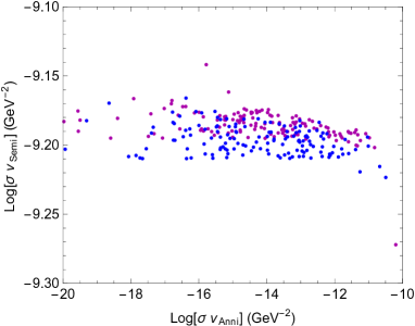
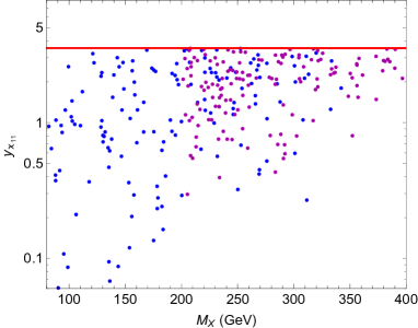
Figure 6: The left plot shows the thermal average $\langle\sigma v_{\rm Anni}\rangle$ for annihilation versus the thermal average $\langle\sigma v_{\rm Semi}\rangle$ for semi-annihilation at the freeze out temperature; The right plot illustrates the allowed region in the plane of $(M_{X},y_{\chi_{11}})$ with the red line signalling the perturbation limit $y_{\chi_{11}}<\sqrt{4\pi}$. The blue points represent the scenario of $m_{H_{1}}=2M_{X}$ (lighter resonance) and the magenta points stand for the scenario of $m_{H_{2}}=2M_{X}$ (heavier resonance). All points satisfy the LFV bounds, neutrino data and Planck satellite measurement $0.117<\Omega h^{2}<0.123$ at 3 $\sigma$ confidential level.

In this section, we will show the numerical analysis to satisfy all the constraints discussed in Section II. We find out that after imposing the LFV bounds and neutrino oscillation data, one DM-neutrino-scalar coupling $y_{\eta_{i1}}$ populates in the range of $(10^{-3},1.0)$, so that the annihilation process in this model can not account for a correct relic density. However a large enhancement for $\langle\sigma v\rangle$ could be achieved if the semi-annihilation proceeds through a $S$-channel and in the vicinity of one narrow-width resonance. Since Eq. (III.15) indicates two resonances of complex scalars are deconstructive, one condition $100<(m_{H_{2}}-m_{H_{1}})<150$ GeV is imposed in the analysis, with the upper limit from the $3\sigma$ EWPT fit at $\cos\alpha=\frac{1}{\sqrt{2}}$. Thus for a given DM mass, only one resonance can effectively be on-shell. On the other hand, we will require $m_{H^{\prime}_{1}}\simeq m_{H^{\prime}_{2}}$, i.e. quasi-degenerate, in order to satisfy the neutrino oscillation data. This condition can be easily fulfilled if we set the mixing term $\lambda^{\prime}_{0}H^{\dagger}\eta^{\prime}s^{\prime*}\varphi^{*}$ to be tiny. In order to simplify the analysis, we adopt several assumptions as below:

$$m_{\eta^{\pm}}=m_{H_{2}},\quad y^{\prime}_{\eta^{\prime}}=y_{\eta^{\prime}},\quad y^{\prime}_{s^{\prime}}=y_{s^{\prime}}$$

$$s_{\alpha}=s_{\alpha^{\prime}}=c_{\alpha}=c_{\alpha^{\prime}}=\frac{1}{\sqrt{2}},$$ (III.18)

We set $m_{\eta^{\pm}}=m_{H_{2}}$ which is consistent with the EWPT bound as shown in Figure 4 and $\ y^{\prime}_{\eta^{\prime}},\ y^{\prime}_{s^{\prime}}$ are taken to be diagonal matrices. Under these assumptions, a numerical scan is conducted for the parameter space by imposing the relevant neutrino and LFV bounds and limiting the relic density to be $0.117<\Omega h^{2}<0.123$. We explore the two on-shell scenarios in two overlapping DM mass regions with $m_{H_{1}}=2M_{X}$ for $80<M_{X}<350$ GeV and $m_{H_{2}}=2M_{X}$ for $200<M_{X}<400$ GeV. Furthermore, in order to work well under the Breit-Wigner narrow width prescription, we remove the points with $\rm{max}(\frac{\Gamma_{H_{1}}}{m_{H_{1}}},\frac{\Gamma_{H_{2}}}{m_{H_{2}}})>0.2$. For the latter case of $m_{H_{2}}=2M_{X}$, we will impose a smaller splitting $(m_{H_{2}}-m_{H_{1}})\simeq(115,125)$ GeV, thus $m_{H_{1}}\gg m_{X}$. This condition will ensure $\Gamma_{H_{1}}\ll m_{H_{1}}$ and avoid co-annihilation from scalars. From the left plot in Fig: 6 we can see that the observed relic density dominantly comes from the semi-annihilation. At the time of freeze out $x_{f}\approx 21.0$ (calculated by Eq.(III.8)), the thermal average of cross section is within the range of $5.98\times 10^{-10}~{}{\rm GeV^{-2}}\lesssim\langle\sigma v_{Semi}\rangle\lesssim 8.83\times 10^{-10}~{}{\rm GeV^{-2}}$, where the larger value normally corresponds to a larger DM mass. In the right plot we show the allowed region in the $(M_{X},y_{\chi_{11}})$ plan with other parameters randomly scanned. The plot demonstrates that a small DM mass $M_{X}<200$ GeV is more sensitive to the lighter $H_{1}+iA_{1}$ resonance and permits a DM Yukawa coupling $y_{\chi_{11}}\gtrsim 0.1$. However for $M_{X}>200$ GeV, our fitting analysis indicates a larger DM coupling $y_{\chi_{11}}\gtrsim 0.5$, which is close to the perturbative limit $\sqrt{4\pi}$ regardless of the lighter or heavier resonance scenario.

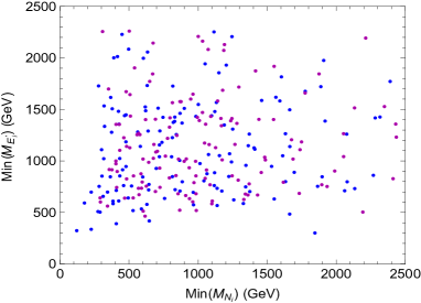
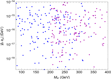
Figure 7: The left plot shows the lightest mass in $M_{E^{\prime}_{i}},i=1,2,3$ versus the lightest mass in $M_{N_{i}},i=1,2,3$; The right plot illustrates the correlation of $|\Delta a_{\mu}|$ to the DM mass $M_{X}$. The blue points represent the scenario of $m_{H_{1}}=2M_{X}$ and the magenta points stand for the scenario of $m_{H_{2}}=2M_{X}$. All points satisfy the LFV bounds, neutrino data and Planck satellite measurement $0.117<\Omega h^{2}<0.123$ at 3 $\sigma$ confidential level.

Fig. 7 presents the mass ranges for $M_{E^{\prime}}(=M_{N^{\prime}})$ and $M_{N}$ which enter into the numerator of neutrino mass form factors as well as values of $|\Delta a_{\mu}|$ versus $M_{X}$. The typical value for the lightest vector-like fermions $L^{\prime}_{i}$ lies in $0.5-2.5$ TeV, but the degeneracy results in no effect on EWPT. Also this mass range of $M_{E^{\prime}}$ is not sensitive to the LHC bound for charged lepton pairs plus missing transverse energy Cai:2018upp . While after enforcing all the bounds, the maximum value for $|\Delta a_{\mu}|$ is of order $\lesssim 10^{-14}$, even lower for most benchmark points, is negligible compared with the $3.6~{}\sigma$ deviation of order $10^{-9}$ as measured by the experiment. Thus this model can not simultaneously account for the large discrepancy in muon $g-2$.

Direct detection: In our case, there are no direction interactions between $H_{1,2}/A_{1,2}$ and quarks at the tree level, therefore the constraints of direct detection searches should be satisfied without difficulty.

IV Conclusions and discussions

We have constructed a neutrino mass model based on hidden local $U(1)_{H}$ symmetry which gives rise to a Dirac fermion type of Dark matter. The neutrino masses are generated at the two-loop level due to the symmetry and particle content. Furthermore because the form factor of the neutrino mass is proportional to the mass squared differences of inert scalars, we require one set of inert scalars to be quasi-degenerate so that a sub-eV scale neutrino mass can be achieved without large fine-tuning for the Yukawa couplings. As variation to this model, we illustrate that the heavy $Z^{\prime}$ associated with the $U(1)$ will not impact the DM annihilation because its mixing with SM $Z$ boson is induced by a complex triplet field $\Delta$, whose VEV is severely constrained by $\rho$-parameter. Particularly, the presence of inert scalars $(\eta,s)$ gives rise to notable $S$ and $T$ deviations. Note that the impact of singlet $s$ on oblique parameters is via the mixing with doublet $\eta$. The $3\sigma$ EWPT fit prefers the mass splitting of $|m_{H_{2}}-m_{H_{1}}|\lesssim 150$ GeV provided $\cos\alpha=\frac{1}{\sqrt{2}}$ and $m_{\eta}^{+}=m_{H_{2}}$.

Our DM is is the lightest neutral particle stabilised by a discrete $\mathbb{Z}_{3}$ parity which is a residual symmetry of $U(1)_{H}$ after spontaneous symmetry breaking. Therefore, in addition to the standard DM annihilation process, DM semi-annihilation is induced in this model. After imposing the LFV bounds and neutrino oscillation data and assuming no specific flavour structure in Yukawa couplings, we find out that the $S-$channel semi-annihilation plays an important role to determine the observed relic density with a DM mass of $\mathcal{O}(100)$ GeV. Our analysis demonstrates that the lighter and heavier resonances can contribute significantly when either one is actually put on-shell and the allowed DM-scalar Yukawa coupling is in the range of ($0.1$-$\sqrt{4\pi}$) depending on the DM mass region.

Appendix A Loop functions for neutrino mass

The neutrino mass in this radiative seesaw model is generated by the two-loop Feynman diagrams in Figure 2. It is convenient to decompose the mass matrix as $(m_{\nu})_{ij}=m_{\nu_{ij}}^{(I)}+m_{\nu_{ij}}^{(II)}+[m_{\nu_{ij}}^{(I)}]^{T}+[m_{\nu_{ij}}^{(II)}]^{T}$, with $m_{\nu_{ij}}^{(I)}$ and $m_{\nu_{ij}}^{(II)}$ calculated to be:

$$m_{\nu}^{(I)} =y_{\eta_{ia}}y_{s^{\prime}_{a\rho}}^{T}y_{\eta^{\prime}_{\rho b}}y_{S_{bj}}^{T}s_{\alpha}c_{\alpha}s^{\prime}_{\alpha}c^{\prime}_{\alpha}\int\frac{d^{4}k_{1}}{(2\pi)^{4}}\int\frac{d^{4}k_{2}}{(2\pi)^{4}}\frac{-M_{N_{\rho}}k_{2}^{2}}{(k_{1}^{2}-M_{N_{\rho}}^{2})(k_{2}^{2}-M_{X_{a}}^{2})(k_{2}^{2}-M_{N^{\prime}_{b}}^{2})}$$

$$\left(\frac{1}{k_{2}^{2}-m_{H_{1}}^{2}}-\frac{1}{k_{2}^{2}-m_{H_{2}}^{2}}\right)\left(\frac{1}{(k_{1}-k_{2})^{2}-m_{H^{\prime}_{1}}^{2}}-\frac{1}{k_{2}^{2}-m_{H^{\prime}_{2}}^{2}}\right)$$ (A.1)

$$m_{\nu}^{(II)} =y_{\eta_{ia}}y_{s^{\prime}_{a\rho}}^{\prime T}y^{\prime}_{\eta^{\prime}_{\rho b}}y_{S_{bj}}^{T}s_{\alpha}c_{\alpha}s^{\prime}_{\alpha}c^{\prime}_{\alpha}\int\frac{d^{4}k_{1}}{(2\pi)^{4}}\int\frac{d^{4}k_{2}}{(2\pi)^{4}}\frac{M_{\chi_{a}}M_{N_{\rho}}M_{N^{\prime}_{b}}}{(k_{1}^{2}-M_{N_{\rho}}^{2})(k_{2}^{2}-M_{X_{a}}^{2})(k_{2}^{2}-M_{N^{\prime}_{b}}^{2})}$$

$$\left(\frac{1}{k_{2}^{2}-m_{H_{1}}^{2}}-\frac{1}{k_{2}^{2}-m_{H_{2}}^{2}}\right)\left(\frac{1}{(k_{1}-k_{2})^{2}-m_{H^{\prime}_{1}}^{2}}-\frac{1}{k_{2}^{2}-m_{H^{\prime}_{2}}^{2}}\right)$$ (A.2)

For clarity, we can redefine $m_{\nu_{ij}}^{(I/II)}=\frac{1}{(4\pi)^{4}}~{}y_{\eta_{ia}}F_{I/II}(H_{1,2},H^{\prime}_{1,2})_{ab}~{}y_{bj}^{T}$ by extracting out a loop factor and Yukawa couplings in the outer loop of Feynman diagrams. After imposing the Feynman parametrisation, the two loop functions $F_{I/II}(H_{1,2},H^{\prime}_{1,2})$ are given by:

$$F_{I}(H_{1,2},H^{\prime}_{1,2})_{ab}=2~{}y^{T}_{s^{\prime}_{a\rho}}M_{N_{\rho}}y_{\eta^{\prime}_{\rho b}}(m^{2}_{H_{1}}-m^{2}_{H_{2}})(m^{\prime 2}_{H_{1}}-m^{\prime 2}_{H_{2}})s_{\alpha}c_{\alpha}s_{\alpha^{\prime}}c_{\alpha^{\prime}}\times$$

$$\int\frac{[da]_{3}[d\alpha]_{5}~{}a(b+c)}{[\alpha(a~{}M^{2}_{N_{\rho}}+b~{}m^{2}_{H^{\prime}_{1}}+c~{}m^{2}_{H^{\prime}_{2}})+a(b+c)(\beta~{}M^{2}_{\chi_{a}}+\gamma~{}M^{2}_{N^{\prime}_{b}}+\rho~{}m^{2}_{H_{1}}+\sigma~{}m_{H_{2}}^{2})]^{2}},$$ (A.3)

$$F_{II}(H_{1,2},H^{\prime}_{1,2})_{ab}=2~{}M_{\chi_{a}}y^{\prime T}_{s^{\prime}_{a\rho}}M_{N_{\rho}}y^{\prime}_{\eta^{\prime}_{\rho b}}M_{N^{\prime}_{b}}(m^{2}_{H_{1}}-m^{2}_{H_{2}})(m^{\prime 2}_{H_{1}}-m^{\prime 2}_{H_{2}})s_{\alpha}c_{\alpha}s_{\alpha^{\prime}}c_{\alpha^{\prime}}\times$$

$$\int\frac{[da]_{3}[d\alpha]_{5}~{}a^{2}(b+c)^{2}}{[\alpha(a~{}M^{2}_{N_{\rho}}+b~{}m^{2}_{H^{\prime}_{1}}+c~{}m^{2}_{H^{\prime}_{2}})+a(b+c)(\beta~{}M^{2}_{\chi_{a}}+\gamma~{}M^{2}_{N^{\prime}_{b}}+\rho~{}m^{2}_{H_{1}}+\sigma~{}m_{H_{2}}^{2})]^{3}},$$ (A.4)

where we use the definitions: $[da]_{3}\equiv\int_{0}^{1}db\int_{0}^{1-b}dc$ with $a=1-b-c$, and $[d\alpha]_{5}\equiv\int_{0}^{1}d\alpha\int_{0}^{1-\alpha}d\beta\int_{0}^{1-\alpha-\beta}d\gamma\int_{0}^{1-\alpha-\beta-\gamma}d\rho$ with $\sigma=1-\alpha-\beta-\gamma-\rho$. Note that these form factors are finite and will be numerically evaluated.

Appendix B T parameter from mixing inert scalars

Since the longitude modes of $W,Z$ gauge bosons are $\partial_{\mu}G^{\pm,0}$, the $T$ parameter is easily calculated from the wave-function renormalisation of Goldstone bosons. We are going to show that two approaches are matching with each other. The relevant terms from the scalar potential are:

$$\mathcal{V} \supset-\mu_{H}^{2}H^{\dagger}H+\lambda_{H}(H^{\dagger}H)^{2}+\lambda_{H\eta}(H^{\dagger}H)(\eta^{\dagger}\eta)+\lambda^{\prime}_{H\eta}(H^{\dagger}\eta)(\eta^{\dagger}H)+\lambda_{\varphi\eta}(\varphi^{\dagger}H)(\eta^{\dagger}\eta)$$

$$+\lambda_{Hs}(H^{\dagger}H)(s^{*}s)+\lambda_{\varphi s}(\varphi^{\dagger}\varphi)(s^{*}s)+(\lambda_{0}H^{\dagger}\eta s^{*}\varphi+h.c.)+\mu_{\eta}^{2}\eta^{\dagger}\eta+\mu_{s}^{2}s^{*}s$$ (B.1)

Due to the $\mathbb{Z}^{3}$ parity, there is no mass splitting among the imaginary and real parts of inert neutral scalars. The masses can be read off from Eq.(B.1):

$$m_{\eta^{+}}^{2}=\mu_{\eta}^{2}+\frac{1}{2}\left(\lambda_{H\eta}v_{H}^{2}+\lambda_{\varphi\eta}v_{\varphi}^{2}\right)$$ (B.2)

$$\frac{1}{2}\begin{pmatrix}s_{R/I}\\ \eta_{R/I}\end{pmatrix}^{T}\left[\begin{array}[]{cc}m_{s_{R}}^{2}&\frac{1}{2}\lambda_{0}v_{H}v_{\varphi}\\ \frac{1}{2}\lambda_{0}v_{H}v_{\varphi}&m_{\eta_{R}}^{2}\\ \end{array}\right]\begin{pmatrix}s_{R/I}\\ \eta_{R/I}\end{pmatrix}$$ (B.5)

with the diagonal parts to be

$$m_{s_{R}}^{2}=\mu_{s}^{2}+\frac{1}{2}\left(\lambda_{Hs}v_{H}^{2}+\lambda_{\varphi s}v_{\varphi}^{2}\right)$$

$$m_{\eta_{R}}^{2}=\mu_{\eta}^{2}+\frac{1}{2}\left(\lambda_{H\eta}v_{H}^{2}+\lambda_{\varphi\eta}v_{\varphi}^{2}+\lambda_{H\eta}^{\prime}v_{H}^{2}\right)$$ (B.6)

The following identities will hold for the mass eigenstates and rotating angle:

$$m_{s_{R}}^{2} = m_{H_{1}}^{2}\cos^{2}\alpha+m_{H_{2}}^{2}\sin^{2}\alpha$$

$$m_{\eta_{R}}^{2} = m_{H_{1}}^{2}\sin^{2}\alpha+m_{H_{2}}^{2}\cos^{2}\alpha$$

$$\sin 2\alpha = \frac{\lambda_{0}v_{H}v_{\varphi}}{m_{H_{1}}^{2}-m_{H_{2}}^{2}}$$ (B.7)

since $\delta\rho=\delta Z_{G^{+}}-\delta Z_{G^{0}}$, the two-point self-energy diagrams in Fig. 8 give us:

$$\hat{\alpha}\Delta T = 2(\lambda_{H\eta}^{\prime}\frac{v_{H}}{2}\sin\alpha+\lambda_{0}\frac{v_{\varphi}}{2}\cos\alpha)^{2}f(m_{H_{1}},m_{\eta^{+}})$$ (B.8)

$$+ 2(\lambda_{H\eta}^{\prime}\frac{v_{H}}{2}\cos\alpha-\lambda_{0}\frac{v_{\varphi}}{2}\sin\alpha)^{2}f(m_{H_{2}},m_{\eta^{+}})$$

$$- \frac{1}{2}\lambda_{0}^{2}v_{\varphi}^{2}f(m_{H_{1}},m_{H_{2}})$$

with the function $f(m_{1},m_{2})=-i\frac{d\Pi(p^{2})}{dp^{2}}|_{p^{2}=0}$, and $\hat{\alpha}=\frac{e^{2}}{4\pi}$. The $\Pi(p^{2})$ is defined as:

$$\Pi(p^{2}) = \int\frac{d^{4}k}{(2\pi)^{4}}\frac{1}{(k^{2}-m_{1}^{2})((k+p)^{2}-m_{2}^{2})}$$ (B.9)

$$= \int\frac{d^{4}k}{(2\pi)^{4}}\int_{0}^{1}dx\frac{1}{(k^{2}-\Delta)^{2}}$$

with $\Delta=-p^{2}(1-x)x+xm_{1}^{2}+(1-x)m_{2}^{2}$. Thus we can obtain the analytic formula:

$$f(m_{1},m_{2}) = \frac{1}{16\pi^{2}}\frac{m_{1}^{4}-m_{2}^{4}+2m_{1}^{2}m_{2}^{2}\log\left(\frac{m_{2}^{2}}{m_{1}^{2}}\right)}{2(m_{1}^{2}-m_{2}^{2})^{3}}$$ (B.10)

Using Eqs.(B.2), (B.6), (B.7), the coefficients in Eq.(B.8) are related to be:

$$(\lambda_{H\eta}^{\prime}\frac{v_{H}}{2}\sin\alpha+\lambda_{0}\frac{v_{\varphi}}{2}\cos\alpha)^{2}=\frac{(m_{H_{1}}^{2}-m_{\eta^{+}}^{2})^{2}}{v_{H}^{2}}\sin^{2}\alpha$$

$$(\lambda_{H\eta}^{\prime}\frac{v_{H}}{2}\cos\alpha-\lambda_{0}\frac{v_{\varphi}}{2}\sin\alpha)^{2}=\frac{(m_{H_{2}}^{2}-m_{\eta^{+}}^{2})^{2}}{v_{H}^{2}}\cos^{2}\alpha$$

$$\lambda_{0}^{2}v_{\varphi}^{2}=\frac{4(m_{H_{1}}^{2}-m_{H_{2}}^{2})^{2}}{v_{H}^{2}}\sin\alpha^{2}\cos^{2}\alpha$$ (B.11)

Then after substituting those identities back to Eq.(B.8), we obtain the $\Delta T$ expression in Eq.(II.64).

Figure 8: Self-energy diagrams for wave-function renormalisation.

Appendix C Inner products for the amplitudes

$$pk=\sqrt{((s-m_{1}^{2}-m_{2}^{2})^{2}-4m_{1}^{2}m_{2}^{2})((s-n_{1}^{2}-n_{2}^{2})^{2}-4n_{1}^{2}n_{2}^{2})},$$

$$p_{1}\cdot k_{1}=\frac{1}{4s}\left(|(s+m_{1}^{2}-m_{2}^{2})(s+n_{1}^{2}-n_{2}^{2})|-pk\cos\theta\right),$$

$$p_{1}\cdot k_{2}=\frac{1}{4s}\left(|(s+m_{1}^{2}-m_{2}^{2})(s+n_{2}^{2}-n_{1}^{2})|+pk\cos\theta\right),$$

$$p_{2}\cdot k_{1}=\frac{1}{4s}\left(|(s+m_{2}^{2}-m_{1}^{2})(s+n_{1}^{2}-n_{2}^{2})|+pk\cos\theta\right),$$

$$p_{2}\cdot k_{2}=\frac{1}{4s}\left(|(s+m_{2}^{2}-m_{1}^{2})(s+n_{2}^{2}-n_{1}^{2})|-pk\cos\theta\right).$$ (C.1)

where $s\equiv(p_{1}+p_{2})^{2}$ is a Mandelstam valuable, $m_{1,2}(p_{1,2})$ are initial state masses(momenta), while $n_{1,2}(k_{1,2})$ are final state masses(momenta).

References

- (1) N. Aghanim et al. [Planck Collaboration], arXiv:1807.06209 [astro-ph.CO].
- (2) E. Ma, Phys. Rev. D 73, 077301 (2006) [hep-ph/0601225].
- (3) B. W. Lee and S. Weinberg, Phys. Rev. Lett. 39, 165 (1977). doi:10.1103/PhysRevLett.39.165
- (4) T. Hambye, JHEP 0901, 028 (2009) doi:10.1088/1126-6708/2009/01/028 [arXiv:0811.0172 [hep-ph]].
- (5) T. Hambye and M. H. G. Tytgat, Phys. Lett. B 683, 39 (2010) doi:10.1016/j.physletb.2009.11.050 [arXiv:0907.1007 [hep-ph]].
- (6) F. D’Eramo and J. Thaler, JHEP 1006, 109 (2010) doi:10.1007/JHEP06(2010)109 [arXiv:1003.5912 [hep-ph]].
- (7) G. Belanger, K. Kannike, A. Pukhov and M. Raidal, JCAP 1204, 010 (2012) doi:10.1088/1475-7516/2012/04/010 [arXiv:1202.2962 [hep-ph]].
- (8) A. Zee, Nucl. Phys. B 264, 99 (1986); K. S. Babu, Phys. Lett. B 203, 132 (1988).
- (9) K. S. Babu and C. Macesanu, Phys. Rev. D 67, 073010 (2003) [hep-ph/0212058].
- (10) E. Ma, Phys. Lett. B 662, 49 (2008) doi:10.1016/j.physletb.2008.02.053 [arXiv:0708.3371 [hep-ph]].
- (11) Y. Kajiyama, H. Okada and K. Yagyu, Nucl. Phys. B 874, 198 (2013) [arXiv:1303.3463 [hep-ph]].
- (12) Y. Kajiyama, H. Okada and T. Toma, Phys. Rev. D 88, 015029 (2013) [arXiv:1303.7356].
- (13) M. Aoki, J. Kubo and H. Takano, Phys. Rev. D 87, no. 11, 116001 (2013) [arXiv:1302.3936 [hep-ph]].
- (14) P. Langacker, Rev. Mod. Phys. 81, 1199 (2009) doi:10.1103/RevModPhys.81.1199 [arXiv:0801.1345 [hep-ph]].
- (15) E. J. Chun and J. C. Park, JCAP 0902, 026 (2009) doi:10.1088/1475-7516/2009/02/026 [arXiv:0812.0308 [hep-ph]].
- (16) P. Ko and T. Nomura, Phys. Rev. D 94, no. 11, 115015 (2016) doi:10.1103/PhysRevD.94.115015 [arXiv:1607.06218 [hep-ph]].
- (17) T. Nomura, H. Okada and P. Wu, JCAP 1805, no. 05, 053 (2018) doi:10.1088/1475-7516/2018/05/053 [arXiv:1801.04729 [hep-ph]].
- (18) E. Ma, I. Picek and B. Radovcic, Phys. Lett. B 726, 744 (2013) doi:10.1016/j.physletb.2013.09.049 [arXiv:1308.5313 [hep-ph]].
- (19) E. Ma, N. Pollard, R. Srivastava and M. Zakeri, Phys. Lett. B 750, 135 (2015) doi:10.1016/j.physletb.2015.09.010 [arXiv:1507.03943 [hep-ph]].
- (20) P. Ko and Y. Tang, JCAP 1501, 023 (2015) doi:10.1088/1475-7516/2015/01/023 [arXiv:1407.5492 [hep-ph]].
- (21) C. Bonilla, R. M. Fonseca and J. W. F. Valle, Phys. Rev. D 92 (2015) no.7, 075028 doi:10.1103/PhysRevD.92.075028 [arXiv:1508.02323 [hep-ph]].
- (22) R. Primulando, J. Julio and P. Uttayarat, arXiv:1903.02493 [hep-ph].
- (23) Z. Maki, M. Nakagawa and S. Sakata, Prog. Theor. Phys. 28, 870 (1962). doi:10.1143/PTP.28.870
- (24) H. Okada and Y. Orikasa, Phys. Rev. D 94, no. 5, 055002 (2016) doi:10.1103/PhysRevD.94.055002 [arXiv:1512.06687 [hep-ph]].
- (25) A. M. Baldini et al. [MEG Collaboration], Eur. Phys. J. C 76, no. 8, 434 (2016) doi:10.1140/epjc/s10052-016-4271-x [arXiv:1605.05081 [hep-ex]].
- (26) B. Aubert et al. [BaBar Collaboration], Phys. Rev. Lett. 104, 021802 (2010) doi:10.1103/PhysRevLett.104.021802 [arXiv:0908.2381 [hep-ex]].
- (27) F. Renga [MEG Collaboration], Hyperfine Interact. 239, no. 1, 58 (2018) doi:10.1007/s10751-018-1534-y [arXiv:1811.05921 [hep-ex]].
- (28) M. Tanabashi et al. [Particle Data Group], Phys. Rev. D 98, no. 3, 030001 (2018). doi:10.1103/PhysRevD.98.030001
- (29) M. E. Peskin and T. Takeuchi, Phys. Rev. D 46, 381 (1992). doi:10.1103/PhysRevD.46.381
- (30) R. Barbieri, L. J. Hall and V. S. Rychkov, Phys. Rev. D 74, 015007 (2006) doi:10.1103/PhysRevD.74.015007 [hep-ph/0603188].
- (31) H. E. Haber and D. O’Neil, Phys. Rev. D 83, 055017 (2011) doi:10.1103/PhysRevD.83.055017 [arXiv:1011.6188 [hep-ph]].
- (32) G. Passarino and M. J. G. Veltman, Nucl. Phys. B 160, 151 (1979). doi:10.1016/0550-3213(79)90234-7
- (33) K. Hagiwara, R. Liao, A. D. Martin, D. Nomura and T. Teubner, J. Phys. G 38, 085003 (2011) doi:10.1088/0954-3899/38/8/085003 [arXiv:1105.3149 [hep-ph]].
- (34) P. Gondolo and G. Gelmini, Nucl. Phys. B 360, 145 (1991). doi:10.1016/0550-3213(91)90438-4
- (35) J. Edsjo and P. Gondolo, Phys. Rev. D 56, 1879 (1997) doi:10.1103/PhysRevD.56.1879 [hep-ph/9704361].
- (36) E. W. Kolb and M. S. Turner, The Early universe, Front. Phys. 69 (1990) 1-547.
- (37) H. Cai, T. Nomura and H. Okada, Nucl. Phys. B 949, 114802 (2019) doi:10.1016/j.nuclphysb.2019.114802 [arXiv:1812.01240 [hep-ph]].