Evolution of scalar and vector cosmological perturbations through a bounce in metric $f(R)$ gravity in flat FLRW spacetime

Abstract

In the present work we present the full treatment of scalar and vector cosmological perturbations in a non-singular bouncing universe in the context of metric $f(R)$ cosmology. Scalar metric perturbations in $f(R)$ cosmology were previously calculated in the Jordan frame, in the present paper we successfully use the Einstein frame to calculate the scalar metric perturbations where the cosmological bounce takes place in the Jordan frame. The Einstein frame picture presented corrects and completes a previous calculation of scalar perturbations and adds new information. Behavior of fluid velocity potential and the pure vector fluid velocity terms are elaborately calculated for the first time in $f(R)$ cosmology for a bouncing universe in presence of exponential gravity. It is shown that the vector perturbations can remain bounded and almost constant during the non-singular bounce in $f(R)$ gravity unlike general relativistic models where we expect the vector perturbations to be growing during the contracting phase and decaying during the expanding phase. The paper shows that the Einstein frame can be used for calculation of scalar and vector metric perturbations in a bouncing universe for most of the cases except the case of asymmetric non-singular bounces.

1 Introduction

Though inflation[1, 2] has been tremendously successful in solving most of the problems of the standard big bang cosmology, the issue of singularity and trans-Planckian problem still remains [3, 4, 5]. A possible solution to the above mentioned problems is to consider the existence of non-singular bouncing cosmologies [6, 7, 8, 9, 10], in which the universe goes from a contracting phase to an expanding one through bounce without any singularity. Non-singular bounce also addresses the horizon and flatness problem[8]. If one does not want to introduce some exotic matter components in a 3-dimensionally flat Friedmann-Lemaitre-Robertson-Walker (FLRW) spacetime then a way of realizing bounce is modifying general relativity (GR) [11, 12, 13, 14, 15, 16]. It is conjectured that GR may not be the unique, correct theory of gravity to describe geometry of space-time when the curvature scale is high. Modifications of the Einstein-Hilbert gravitational action by higher order curvature invariants is done in very strong gravity regimes, such as in very early universe. At high curvature limits, when bounce happens, modifications to GR is expected. In this paper we study perturbations in a bouncing cosmology where the theory of gravity is given by metric $f(R)$ theory. The $f(R)$ paradigm is important as various models of inflation and late time acceleration of the universe can be modelled on $f(R)$ gravity theories. Current observation has detected a cosmic acceleration starting after the matter domination. Modified gravity theories [17, 18, 19, 20] have been used to explain this late time acceleration of the universe. Although $f(R)$ gravity [21] [22] is only one amongst the many modified gravity models, but it is one of the simplest modifications of GR which can tackle various cosmological problems.

It is known that $f(R)$ theory of gravity can be analyzed [13, 23, 24, 25] in two conformal frames; the Jordan frame and the Einstein frame. In Jordan frame the theory is a higher derivative theory, because higher than two order of time derivatives appear in the field equation. The Jordan frame field equation is obtained by varying the $f(R)$ action with respect to the metric tensor [24]. In $f(R)$ cosmology is is assumed that the problem of cosmological dynamics is fundamentally posed in the Jordan frame although one can work the cosmological dynamics also in the Einstein frame using the conformal transformation connecting the frames. An advantage of working in the Einstein frame is that the theory of gravity becomes GR and known techniques of GR evolution can be applied in the Einstein frame. One can always transform back to the Jordan frame after calculating cosmological dynamics in the Einstein frame. In previous studies this was the method followed [13]. Einstein frame description of $f(R)$ is GR with an added scalar field that is minimally coupled to gravity and non-minimally coupled to matter. Einstein frame description of $f(R)$ gravity provides easier ways to tackle many problems in $f(R)$ gravity.

There have been many attempts to realize bounce in various $f(R)$ gravity models [15] [12]. It was pointed out in [16] that exponential $f(R)$ theory might be a good candidate theory which supports a bounce in flat FLRW metric. We will, hence, deal with exponential $f(R)$ gravity in this paper. The present work deals with scalar and vector perturbations in a bouncing universe guided by exponential gravity, the bounce takes place in the Jordan frame. The perturbations have been calculated in both the Jordan and Einstein frames and then the results are matched to gain insight into the nature of the conformal correspondence of the two frames. It has been shown that the Einstein frame can be used for the calculation of scalar cosmological perturbations for symmetric bounce in the Jordan frame. The conformal correspondence fails for asymmetrical bounces in the Jordan frame. No such difficulties arise for vector perturbations where the Einstein frame can be safely used for all the calculations in a much easier way. A part of scalar metric perturbation calculation in the Einstein frame was incompletely presented in an earlier work Ref. [13] where the authors did not take into account the role of fluid velocity potential. In the present work we specify the complete and correct way of calculation of the scalar metric perturbations in a bouncing universe using the Einstein frame. We present the full nature of the scalar perturbations and the dynamics of the fluid velocity potential during a cosmological bounce. The next part of the paper shows the nature of vector metric perturbations during a non-singular bounce. In $f(R)$ cosmology the vector perturbations remains almost constant during the bounce which differs from GR results where the vector perturbations generally increases during the contraction phase [26]. Throughout the paper the role of the Einstein frame as an important frame for calculations has been emphasized. The issue about tensor perturbations in a bouncing universe will be addressed in a future work.

The material in the paper is presented in the following manner. The next section presents the background cosmological evolution in both the Jordan frame and Einstein frame. It also specifies the conformal transformation relating these frames. Section 3 introduces the scalar metric perturbations in both the frames. The Jordan frame result is first calculated and next the Einstein frame results are presented. The results of scalar perturbations are calculated for both a symmetric and asymmetric bounce in the Jordan frame. The topic of vector perturbations is taken up in section 4. The next and the last section concludes the present work with a brief summary of the results obtained.

2 Field equations of $f(R)$ gravity

In the following we work with the spatially flat maximally symmetric FLRW metric given by

$$ds^{2}=-dt^{2}+a^{2}(t)d{\bf x}^{2}$$ (1)

where $t$ is the cosmological time, ${\bf x}$ is the Co-moving spatial coordinates and $a(t)$ is the scale-factor of the universe. In the domain of general relativity it is well known that a bouncing solution is possible only for spatially positively curved FLRW universe, if we do not want to include any exotic matter component in the scenario. But in metric $f(R)$ gravity and as shown in some previous works[13, 14], it is possible to have bouncing solution in spatially flat FLRW universe without invoking any exotic matter component for certain $f(R)$ theories, simplest of which being the $R+\alpha R^{2}$ gravity with a negative $\alpha$. The reason is that the extra curvature induced energy density and pressure terms can indeed produce the bouncing conditions. In this section we present the field equations in Jordan and Einstein frame respectively. We will later apply the formalism to study classical cosmological bounce phenomena [9].

2.1 The relevant cosmological equations in Jordan and Einstein frames

The modified Friedmann equations for $f(R)$ theory in the Jordan frame are given as [24]:

$$3H^{2} = \frac{\kappa}{F(R)}\rho_{\rm eff}\,,$$ (2)

$$3H^{2}+2\dot{H} = -\frac{\kappa}{F(R)}P_{\rm eff}\,,$$ (3)

where $H$ is the conventional Hubble parameter defined as $H\equiv\dot{a}/a$ and the constant $\kappa=8\pi G$ where $G$ is the universal gravitational constant. In the above equations

$$F(R)\equiv\frac{df(R)}{dR}\,.$$ (4)

The dot specifies a derivative with respect to cosmological time $t$. The effective energy density, $\rho_{\rm eff}$, and pressure, $P_{\rm eff}$, are defined as:

$$\rho_{\rm eff}\equiv\rho+\rho_{\rm curv}\,,\,\,\,\,\,P_{\rm eff}\equiv P+P_{\rm curv}\,,$$ (5)

where $\rho_{\rm curv}$ and $P_{\rm curv}$ are given by

$$\rho_{\rm curv} \equiv \frac{RF-f}{2\kappa}-\frac{3H\dot{R}F_{R}(R)}{\kappa}\,,$$ (6)

$$P_{\rm curv} \equiv \frac{\dot{R}^{2}F_{RR}+2H\dot{R}F_{R}+\ddot{R}F_{R}}{\kappa}-\frac{RF-f}{2\kappa}\,,$$ (7)

which are curvature induced energy-density and pressure. In the above equations the subscript $R$ specifies derivatives with respect to the Ricci scalar $R$. The curvature induced thermodynamic variables exists in absence of any hydrodynamic matter. The conventional $\rho$ and $P$ are defined through

$$T_{\mu\nu}=(\rho+P)u_{\mu}u_{\nu}+Pg_{\mu\nu}\,,$$ (8)

which has the information of hydrodynamic matter. In this article we assume the fluid to be barotropic so that its equation of state is

$$P=\omega\rho\,,$$ (9)

where $\omega$ is a constant and its value is zero for dust and one-third for radiation. It must be noted that $u_{\mu}$ in Eq. (8) is the 4-velocity of a fluid element and $u_{\mu}u^{\mu}=-1\,.$

One can make a conformal transformation on the system of equations in the Jordan frame to recast the problem in the Einstein frame. The Einstein frame version of the cosmological dynamics sometimes becomes relatively easy to manage as in this version one deals with the known Einstein equations. The Einstein frame description of $f(R)$ gravity is obtained by the following conformal transformation,

$$\tilde{g}_{\mu\nu}=F(R)g_{\mu\nu}\,,$$ (10)

and simultaneously defining a new scalar field $\phi$ as

$$\phi=\sqrt{\frac{3}{2\kappa}}\ln F(R)\,.$$ (11)

This scalar field plays an important role in the Einstein frame. The conformally transformed line element in the Einstein frame is

$$d\tilde{s}^{2}=-d\tilde{t}^{2}+\tilde{a}^{2}d{\bf x}^{2}\,,$$ (12)

where the time coordinate, $\tilde{t}$, and the scale factor, $\tilde{a}$, in the Einstein frame are related to their corresponding Jordan frame terms via the relations

$$d\tilde{t}=\sqrt{F(R)}\,dt\,\,\,\,\,{\rm and}\,\,\,\,\,\tilde{a}(t)=\sqrt{F(R)}\,a(t)\,.$$ (13)

Using these transformations one can formulate the gravitational dynamics of $f(R)$ gravity in the Einstein frame in presence of matter and the scalar field $\phi$ acting as sources. The energy-momentum tensor in the Einstein frame, which is related to $T^{\mu\nu}$ in the Jordan frame, turns out to be

$$\tilde{T}_{\mu\nu}=(\tilde{\rho}+\tilde{P})\tilde{u}_{\mu}\tilde{u}_{\nu}+\tilde{P}\tilde{g}_{\mu\nu}\,,$$ (14)

where $\tilde{\rho}=\rho/F^{2}(R)$, $\tilde{P}=P/F^{2}(R)$ and $\tilde{u}_{\mu}=\sqrt{F(R)}u_{\mu}$. In the Einstein frame $\tilde{g}^{\mu\nu}\tilde{u}_{\mu}\tilde{u}_{\nu}=-1$. Except $\tilde{T}^{\mu\nu}$, the energy-momentum tensor for the scalar field also acts as source of curvature in the Einstein frame and it is given as

$$S^{\mu}_{\nu}=\partial_{\alpha}\phi\partial_{\nu}\phi\tilde{g}^{\alpha\mu}-\delta^{\mu}_{\nu}{\mathcal{L}}(\phi)\,,$$ (15)

where the scalar field Lagrangian is

$${\mathcal{L}}(\phi)=\frac{1}{2}\partial_{\alpha}\phi\partial_{\beta}\phi\tilde{g}^{\alpha\beta}+V(\phi)\,.$$ (16)

The scalar field potential in the Einstein frame turns out to be

$$V(\phi)=\frac{RF-f}{2\kappa F^{2}}\,,$$ (17)

where one has to express $R=R(\phi)$, from Eq. (11) by inverting it, and then express $V(\phi)$ as an explicit function of $\phi$. From the form of $S^{\mu}_{\nu}$ one can write

$$S^{0}_{0}\equiv\rho_{\phi}=\frac{1}{2}\left(\frac{d\phi}{d\tilde{t}}\right)^{2}+V(\phi)\,,\,\,\,\,S^{i}_{i}\equiv P_{\phi}=\frac{1}{2}\left(\frac{d\phi}{d\tilde{t}}\right)^{2}-V(\phi)\,,$$ (18)

where the scalar field $\phi$ is assumed to be a function of time only. The total energy-momentum tensor responsible for gravitational effects in the Einstein frame is $\tilde{T}^{\mu}_{\,\,\,\,\nu}+S^{\mu}_{\,\,\,\,\nu}$ which is a mixed tensor with only diagonal components.

The time coordinate, $t$, and the Hubble parameter, $H$, in the the Jordan frame are related to the time coordinate, $\tilde{t}$, and Hubble parameter $\tilde{H}(\equiv\frac{1}{\tilde{a}}\frac{d\tilde{a}}{d\tilde{t}})$, in the Einstein frame via the relations:

$$\tilde{t}=\int_{t_{0}}^{t}\sqrt{F(R)}dt^{\prime}\,,\,\,\,\,\,\,\,H=\sqrt{F}\left(\tilde{H}-\sqrt{\frac{\kappa}{6}}\,\frac{d\phi}{d\tilde{t}}\right)\,.$$ (19)

As we will be interested mainly in bouncing cosmologies $t_{0}$ will be set to zero. The instant $t_{0}=0$ is the bouncing time in the Jordan frame. The Einstein frame description of cosmology can be tackled like FLRW spacetime in presence of a fluid and a scalar field. The presence of the Scalar field potential $V(\phi)$ gives one a pictorial understanding of the physical system which is lacking in the Jordan frame. Seeing the nature of the potential and the initial conditions of the problem one gets a hint about the possible time development of the system. The time evolution of the scalar field in the Einstein frame is dictated by the equation

$$\frac{d^{2}\phi}{d\tilde{t}^{2}}+3\tilde{H}\frac{d\phi}{d\tilde{t}}+\frac{dV}{d\phi}=\sqrt{\frac{\kappa}{6}}(1-3\omega)\tilde{\rho}\,,$$ (20)

where the equation of state of the fluid in the Jordan frame is $P=\omega\rho$. It is interesting to note that the equation of state of the fluid remains the same in the Einstein frame. The evolution of the energy density in the Einstein frame is given by

$$\frac{d\tilde{\rho}}{d\tilde{t}}+\sqrt{\frac{\kappa}{6}}(1-3\omega)\tilde{\rho}\frac{d\phi}{d\tilde{t}}+3\tilde{H}\tilde{\rho}(1+\omega)=0\,.$$ (21)

The above two equations dictate the time evolution of $\tilde{\rho}$ and $\phi$ in the Einstein frame. To generate proper bouncing solution from the above two equations one requires the values of only two quantities at the bouncing time, they are $\phi(\tilde{t}_{0})$, $\left(\frac{d\phi}{d\tilde{t}}\right)_{\tilde{t}_{0}}$, the other parameters are determined from these two at the bouncing time[13]. In general for a flat FLRW spacetime these two values of the respective quantities are enough to solve the whole system in the Einstein frame. The expression of the Hubble parameter and its rate of change in the Einstein frame are given as

$$\tilde{H}^{2} = \frac{\kappa}{3}(\rho_{\phi}+\tilde{\rho})\,,$$ (22)

$$\frac{d\tilde{H}}{d\tilde{t}} = -\frac{\kappa}{2}\left[\left(\frac{d\phi}{d\tilde{t}}\right)^{2}+(1+\omega)\tilde{\rho}\right]\,.$$ (23)

3 Scalar cosmological perturbations in $f(R)$ gravity

Scalar perturbation in the cosmological framework, mainly related to inflation, has been widely studied [27, 28, 29, 30]. In this section we discuss the evolution of scalar cosmological perturbation through a bounce in $f(R)$ gravity both in Jordan frame and Einstein frame. For the sake of comparison, it is better to use the conformal time $\eta$, since by definition it is invariant under a conformal transformation, $d\eta={dt}/{a(t)}={d\tilde{t}}/{\tilde{a}(\tilde{t})}$. The most general form of the line element in the Jordan frame is:

$$ds^{2}=a(\eta)^{2}[-(1+2\chi)d\eta^{2}+2B_{,i}dx^{i}d\eta+((1-2\psi)\delta_{ij}+2E_{,ij})dx^{i}dx^{j}]\,.$$ (24)

Here $\chi$, $B$, $\psi$ and $E$ are functions of space and time. The subscript(s) preceded by a comma specifies partial derivatives. The corresponding expression in Einstein frame for the perturbed spacetimes is:

$$d\tilde{s}^{2}=(F+\delta F)ds^{2}=\tilde{a}(\eta)^{2}[-(1+2\tilde{\chi})d\eta^{2}+2\tilde{B}_{,i}dx^{i}d\eta+((1-2\tilde{\psi})\delta_{ij}+2\tilde{E}_{,ij})dx^{i}dx^{j}],$$ (25)

where henceforth $F$ stands for the unperturbed value of $df/dR$. The scale-factors are still related via the relation specified in Eq. (13). The scalar metric perturbation functions in the two frames are related via [25],

$$\tilde{\chi}=\chi+\frac{\delta F}{2F}\,, {\rm and} \tilde{\psi}=\psi-\frac{\delta F}{2F}\,,$$ (26)

$$\tilde{B}=B\,, {\rm and} \tilde{E}=E\,.$$ (27)

In Jordan frame the gauge-invariant variables are:

$$\Phi=\chi+\frac{1}{a}[(B-E^{\prime})a)]^{\prime}\,,\,\,\,\,\Psi=\psi-\frac{a^{\prime}}{a}(B-E^{\prime})\,.$$ (28)

The corresponding gauge-invariant variables, in the Einstein frame, are:

$$\tilde{\Phi}=\tilde{\chi}+\frac{1}{\tilde{a}}[(\tilde{B}-\tilde{E}^{\prime})\tilde{a})]^{\prime}=\Phi+\frac{\delta F^{(gi)}}{2F}\,,\,\,\,\,\,\tilde{\Psi}=\tilde{\psi}-\frac{\tilde{a}^{\prime}}{\tilde{a}}(\tilde{B}-\tilde{E}^{\prime})=\Psi-\frac{\delta F^{(gi)}}{2F}\,,$$ (29)

where $\delta F^{(gi)}=(\partial F/\partial R)\delta R^{(gi)}$. The gauge invariant perturbation of a scalar quantity $q$ is [29], $\delta q^{(gi)}\equiv\delta q+q^{\prime}(B-E^{\prime})\,.$ Here the primes stand for derivatives with respect to conformal time. Assuming the perturbation in the matter sector in Jordan frame to be such that

$$\delta P^{(gi)}-c_{s}^{2}\delta\rho^{(gi)}=0\,,$$ (30)

where $c_{s}^{2}={\delta P}/{\delta\rho}$ one can derive the relation between $\tilde{P}^{(gi)}$ and $\tilde{\rho}^{(gi)}$ in the Einstein frame as

$$\delta\tilde{P}^{(gi)}-c_{s}^{2}\delta\tilde{\rho}^{(gi)} = \delta\tilde{P}-c_{s}^{2}\delta\tilde{\rho}$$ (31)

$$= \delta(Pe^{-2\sqrt{\frac{2\kappa}{3}}\phi})-c_{s}^{2}\delta(\rho e^{-2\sqrt{\frac{2\kappa}{3}}\phi})$$

$$= e^{-2\sqrt{\frac{2\kappa}{3}}\phi}(\delta P-c_{s}^{2}\delta\rho)+2\sqrt{\frac{2\kappa}{3}}e^{-2\sqrt{\frac{2\kappa}{3}}\phi}(c_{s}^{2}\rho-P)\delta\phi$$

$$= e^{-2\sqrt{\frac{2\kappa}{3}}\phi}(\delta P^{(gi)}-c_{s}^{2}\delta\rho^{(gi)})+2\sqrt{\frac{2\kappa}{3}}e^{-2\sqrt{\frac{2\kappa}{3}}\phi}(c_{s}^{2}\rho-P)\delta\phi$$

$$= 2\sqrt{\frac{2\kappa}{3}}\tilde{\rho}(c_{s}^{2}-\omega)\delta\phi\,,$$

showing that for a single barotropic fluid (where $\omega=c_{s}^{2}$) whose equation of state is given by Eq. (9) in the Jordan frame one must have $\delta\tilde{P}^{(gi)}-c_{s}^{2}\delta\tilde{\rho}^{(gi)}=0$ in the Einstein frame.

Before we proceed to formulate the scalar cosmological perturbation in the Jordan and Einstein frames it is pertinent to elucidate the nature of gauge choices and their relationship with conformal transformations. If we apply synchronous gauge in Jordan frame, one should impose $\chi=B=0$. It can be noted that although $\tilde{B}=B=0$ in Einstein frame, $\tilde{\chi}$ does not vanish. So the definition of synchronous gauge is not the same in both frames.

In the spatially-flat gauge, in Jordan frame, one has to impose $\chi=E=0$. From Eq. (26) it is seen that $\tilde{\chi}$ does not vanish in Einstein frame. Consequently the spatially-flat gauge is also not conformally invariant.

Only in the longitudinal gauge, where one imposes $B=E=0$ in the Jordan frame, one obtains $\tilde{B}=\tilde{E}=0$ in Einstein frame. The longitudinal gauge remains invariant under the conformal transformation connecting the Jordan frame and the Einstein frame. Hence we will use longitudinal gauge in the present article from here on.

3.1 Scalar perturbations in the Jordan frame

In the domain of linear perturbations, the scalar perturbed FLRW metric has two gauge invariant degrees of freedom. In the longitudinal gauge this can be expressed as,

$$ds^{2}=a^{2}(\eta)\left[-(1+2\Phi)d\eta^{2}+(1-2\Psi)\delta_{ij}dx^{i}dx^{j}\right]$$ (32)

Here $\Phi$ and $\Psi$ are the two gauge invariant perturbation degrees of freedom, also called the Bardeen potentials. The, $00$, $ii$, $ij-th(i\neq j)$ elements of the linearized perturbed Einstein equation in the Fourier space are [31]:

$$F[-k^{2}(\Phi+\Psi)-3\mathcal{H}(\Phi^{\prime}+\Psi^{\prime})+(3\mathcal{H}^{\prime}-6\mathcal{H}^{2})\Phi-3\mathcal{H}^{\prime}\Psi]$$

$$+F^{\prime}(-9\mathcal{H}\Phi+3\mathcal{H}\Psi-3\Psi^{\prime})=\kappa a^{2}\delta\rho\,,$$ (33)

$$F[\Phi^{\prime\prime}+3\mathcal{H}(\Phi^{\prime}+\psi^{\prime})+3\mathcal{H}^{\prime}+(\mathcal{H}^{\prime}+2\mathcal{H}^{2})\Psi]+F^{\prime}(3\mathcal{H}\Phi-\mathcal{H}\Psi+3\Phi^{\prime})$$

$$+F^{\prime\prime}(3\Phi-\Psi)=c_{s}^{2}\kappa a^{2}\delta P\,,$$ (34)

$$\Phi-\Psi-\frac{2F_{R}}{a^{2}F}[3\Psi^{\prime\prime}+6(\mathcal{H}^{\prime}+\mathcal{H}^{2})\Phi+3\mathcal{H}(\Phi^{\prime}+3\Psi^{\prime})-k^{2}(\Phi-2\Psi)]=0\,,$$ (35)

where $F_{R}=dF/dR$. If there is only a single matter component present, the perturbation in the matter sector can be assumed to be adiabatic, so that the sound velocity can be defined as done in the beginning of this section. Using Eq. (33) and (34), we can write

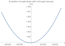
Figure 1: Evolution of scale factor with $\eta$ through asymmetric bounce

$$(1+F)\left[\Phi^{\prime\prime}+\Psi^{\prime\prime}+3\mathcal{H}(1+c_{s}^{2})(\Phi^{\prime}+\Psi^{\prime})+c_{s}^{2}(k^{2}+6\mathcal{H}^{2})\Phi+3\mathcal{H}^{\prime}(1-c_{s}^{2})\Phi+\mathcal{H}^{\prime}(1+c_{s}^{2})\Psi\right.$$

$$+\left.(2\mathcal{H}^{2}+c_{s}^{2}k^{2})\Psi\right]+F^{\prime}[\mathcal{H}(1+3c_{s}^{2})(\Phi-3\Psi)+3\Phi^{\prime}+3c_{s}^{2}\Psi^{\prime}]+F^{\prime\prime}(3\Phi-\Psi)=0\,.$$ (36)

A form of the above perturbation equations of $f(R)$ gravity in the Jordan frame was also calculated in [32] where the authors studied the problem of structure formation in late times. In this paper we will follow the equations as written above and obtained from [31] which seem more appropriate for our analysis. Eq. (35) and (36) can be solved numerically to get the solutions $\Phi$ and $\Psi$. In the present article we will exclusively work with exponential gravity [16] where the form of $f(R)$ is given as

$$f(R)=\frac{1}{\alpha}\exp{(\alpha R)}\,,$$ (37)

where $\alpha=10^{12}$ for phenomenological reasons, it sets the energy scale of bounce. In the present work all the values of dimensional constants (as $\alpha$) or variables (as ${\cal H}$, $\eta$, and others) will be represented in Planck units. To go back to mass units one has to multiply the appropriate variables by suitable power of Planck mass expressed in GeV units. We choose exponential gravity as in this case the gravitational theory does not have any instabilities, as because with $\alpha>0$ we have

$$F>0\,,\,\,\,\,\,F_{R}>0\,.$$

The issues about instability in this kind of theory is discussed in [16].

Figure 2: Evolution of $\Phi$ with $\eta$ through asymmetric bounce, calculated directly in Jordan frame

Figure 3: Evolution of $\Psi$ with $\eta$ through asymmetric bounce, calculated directly in Jordan frame

The blue curves in Fig. 7 and Fig. 7 shows the evolution of $\Phi(k,\eta)$ and $\Psi(k,\eta)$ for $k=10^{-10}$ for a particular background evolution. We have used $\Phi(0)=0.0001$, $\Phi^{\prime}(0)=0,\Psi(0)=0.0002,\Psi^{\prime}(0)=0$ to produce the plots. The bouncing time is $\eta=0$. For the background we have chosen radiation where $\omega=1/3$. The bounce in the background is shown in Fig. 1 where the scale-factor is plotted with respect to $\eta$. To obtain the the background solutions we have initially solved the system of equations as specified in the initial part of section 2 in Jordan frame. The analysis is done in coordinate time. Later the result is transformed to conformal time. The conditions used to produce the bouncing background solution are, ${\cal H}(0)=0$, ${\cal H}^{\prime}(0)=6.8\times 10^{-14}$ and ${\cal H}^{\prime\prime}=0$. The background evolution in Fig. 1 specifies a symmetric bounce. In all the calculations of bounce we have normalized the scale-factor in the Jordan frame in such a way that $a(0)=1$. One can also choose the bounce in the background to be asymmetric. In this case the conditions at $\eta=0$ remains the same as before (as in the symmetric case) except that ${\cal H}^{\prime\prime}(0)\neq 0$. The asymmetry in the background evolution can be generated from an infinitesimal value of the second time derivative of the Hubble parameter as ${\cal H}^{\prime\prime}(0)=8.2\times 10^{-21}$. The perturbation evolution in an asymmetric background in the Jordan frame are plotted in Fig. 3 and Fig. 3. To evaluate the dynamics of the perturbations the values of the perturbations are now not specified at $\eta=0$ but at $\eta=-10^{6}$. The reason for choosing a separate time instant for plotting the asymmetric bounce results will become clear when we analyze the case of asymmetric bounces in the Einstein frame. In the present case $\Phi(-10^{6})=0.7$, $\Psi(-10^{6})=0.9$ and $\Phi^{\prime}(-10^{6})=\Psi^{\prime}(-10^{6})=0$ and the plots show perturbation evolution for $k=10^{-10}$. The plots of the perturbation evolution in the Jordan frame are visibly continuous and smooth. We will see later that if we try to get these results from the Einstein frame calculation we will hit localized singularities.

In the next section we will try to recast the problem in the Einstein frame. A part of this calculation was incompletely done in an earlier publication [13] where the authors disregarded the velocity potential of the fluid in the Einstein frame. In the present work we complete and rectify the previous calculation.

3.2 Einstein frame

In Einstein frame the scalar perturbation in the longitudinal gauge is given as

$$d\tilde{s}^{2}=\tilde{a}^{2}(\eta)\left[-(1+2\tilde{\Phi})d\eta^{2}+(1-2\tilde{\Psi})\delta_{ij}dx^{i}dx^{j}\right]\,.$$ (38)

In Einstein frame the gravitational theory is essentially GR and the energy-momentum tensor of the hydrodynamic matter and the scalar field are both diagonal, it is easy to check from the $ij-{\rm th}(i\neq j)$ component of the perturbed field equation that

$$\tilde{\Phi}=\tilde{\Psi}\,.$$ (39)

This is different from the behavior of the above quantities in the Jordan frame, because the energy-momentum tensor of the existing matter component being diagonal does not necessarily implies the equality of the two Bardeen potentials in a higher derivative gravity theory. This is a good instance where switching to the Einstein frame makes things easier. The Jordan frame Bardeen potentials can be recovered from the Einstein frame Bardeen potential as follows [29],

$$\Phi=-\frac{2}{3}\left(\frac{F^{2}}{F^{\prime}a}\right)\left[\left(\frac{a}{F}\right)\tilde{\Phi}\right]^{\prime}\,,\,\,\,\,\Psi=\frac{2}{3}\left(\frac{1}{FF^{\prime}a}\right)(aF^{2}\tilde{\Phi})^{\prime}\,.$$ (40)

Later it will be shown that these connecting formulae breaks down in the case of asymmetric bounce in the Jordan frame.

As the velocity potential cannot be in general neglected when treating the scalar metric perturbations we rewrite the perturbation equations using this new information. Perturbed Einstein tensor components are:

$$\delta G^{0}_{0} = \frac{2}{\tilde{a}^{2}}[-3\tilde{\mathcal{H}}(\tilde{\mathcal{H}}\tilde{\Phi}+\tilde{\Phi}^{\prime})+\nabla^{2}\tilde{\Phi}]\,,$$ (41)

$$\delta G^{0}_{i} = \frac{2}{\tilde{a}^{2}}\left[\tilde{\Phi}^{\prime}+\tilde{\mathcal{H}}\tilde{\Phi}\right]_{,i}\,,$$ (42)

$$\delta G^{i}_{j} = -\frac{2}{\tilde{a}^{2}}[(2\tilde{\mathcal{H}}^{\prime}+\tilde{\mathcal{H}}^{2})\tilde{\Phi}+3\tilde{\mathcal{H}}\tilde{\Phi}^{\prime}+\tilde{\Phi}^{\prime\prime}]\delta^{i}_{j}\,.$$ (43)

Here a partial derivative with spatial coordinates is specified with the comma followed by a Latin alphabet. Perturbed energy-momentum tensor components for hydrodynamic matter are [29]:

$$\delta\tilde{T}_{0}^{0} = \delta\tilde{\rho}\,,$$ (44)

$$\delta\tilde{T}_{i}^{0} = (\tilde{\rho}+\tilde{P})\tilde{a}^{-1}\delta\tilde{u}_{i}=-(\tilde{\rho}+\tilde{P})\tilde{a}^{-1}\partial_{i}\tilde{U}\,,$$ (45)

$$\delta\tilde{T}_{j}^{i} = -\delta\tilde{P}\delta^{i}_{j}\,.$$ (46)

The quantity $\tilde{U}$ is the velocity potential given by $\delta\tilde{u}_{i}=-\partial_{i}\tilde{U}+\tilde{v}_{i}$. Here $\tilde{v}_{i}$ is is the pure vector part of the fluid velocity perturbation in the Einstein. The perturbed scalar field energy momentum tensor components are:

$$\delta S_{0}^{0} = a^{-2}\left(-{\phi^{\prime}}^{2}\tilde{\Phi}+\phi^{\prime}\delta\phi^{{\prime}}+\tilde{a}^{2}V_{,\phi}\delta\phi\right)\,,$$ (47)

$$\delta S_{i}^{0} = a^{-2}\phi^{\prime}\delta\phi_{,i}\,,$$ (48)

$$\delta S_{j}^{i} = -a^{-2}\left(-\tilde{\Phi}{\phi^{\prime}}^{2}+\phi^{\prime}\delta\phi^{\prime}-\tilde{a}^{2}V_{,\phi}\delta\phi\right)\delta^{i}_{j}\,.$$ (49)

A derivative with respect to $\phi$ is specified by a comma followed by $\phi$ in the subscript. Using the results we can write the perturbed Einstein equations as:

$$-3\tilde{\mathcal{H}}(\tilde{\mathcal{H}}\tilde{\Phi}+\tilde{\Phi}^{\prime})+\nabla^{2}\tilde{\Phi} = \frac{\kappa}{2}\left(\tilde{a}^{2}\delta\tilde{\rho}-{\phi^{\prime}}^{2}\tilde{\Phi}+\phi^{\prime}\delta\phi^{\prime}+\tilde{a}^{2}V_{,\phi}\delta\phi\right)\,,$$ (50)

$$(2\tilde{\mathcal{H}}^{\prime}+\tilde{\mathcal{H}}^{2})\tilde{\Phi}+\tilde{\Phi}^{\prime\prime}+3\tilde{\mathcal{H}}\tilde{\Phi}^{\prime} = \frac{\kappa}{2}\left(\tilde{a}^{2}\delta\tilde{P}-\tilde{\Phi}{\phi^{\prime}}^{2}+\phi^{\prime}\delta\phi^{\prime}-\tilde{a}^{2}V_{,\phi}\delta\phi\right)\,,$$ (51)

$$\frac{\kappa}{2}\left[\phi^{\prime}\delta\phi-\tilde{a}(\tilde{\rho}+\tilde{p})\tilde{U}\right] = \tilde{\Phi}^{\prime}+\tilde{\mathcal{H}}\tilde{\Phi}\,.$$ (52)

Multiplying the first of the above set of equations by $c_{s}^{2}$ and subtracting from the second one yields,

$$\tilde{\Phi}^{\prime\prime}-c_{s}^{2}\nabla^{2}\tilde{\Phi}+\left(2\tilde{\mathcal{H}}^{\prime}+\tilde{\mathcal{H}}^{2}\right)\tilde{\Phi}+3\tilde{\mathcal{H}}\tilde{\Phi}^{\prime}+3c_{s}^{2}\tilde{\mathcal{H}}\left(\tilde{\mathcal{H}}\tilde{\Phi}+\tilde{\Phi}^{\prime}\right)$$

$$=-\frac{\kappa}{2}\tilde{\Phi}\phi^{\prime 2}\left(1-c_{s}^{2}\right)+\frac{\kappa}{2}\phi^{\prime}(1-c_{s}^{2})\delta{\phi}^{\prime}-\frac{\kappa\tilde{a}^{2}}{2}V_{,\phi}(1+c_{s}^{2})\delta\phi\,.$$ (53)

This is one equation which gives the dynamics of the perturbed potential $\tilde{\Phi}$ in the Einstein frame. The scalar field perturbation is linked with the above dynamics. We require more equations for uniquely solving the perturbation evolutions.

The other equation comes from perturbing the Klein-Gordon equation as:

$$\tilde{\Box}\phi-V_{,\phi}+\frac{1}{\sqrt{-\tilde{g}}}\frac{\partial\mathcal{L_{M}}}{\partial\phi}=0\,,$$ (54)

where $\tilde{\Box}\equiv\tilde{D}^{\mu}\tilde{D}_{\mu}$, $\tilde{D}_{\mu}$ being the covariant derivative in the Einstein frame. Here $\mathcal{L_{M}}$ specifies the Lagrangian of the hydrodynamic fluid. Using the following fact we can write down the last term on the left hand side of the above equation,

$$\frac{\partial\mathcal{L_{M}}}{\partial\phi}=\frac{\partial\mathcal{L_{M}}}{\partial g^{\mu\nu}}\frac{\partial g^{\mu\nu}}{\partial\phi}=\frac{1}{F(\phi)}\frac{\partial\mathcal{L_{M}}}{\partial\tilde{g}^{\mu\nu}}\frac{\partial(F(\phi)\tilde{g}^{\mu\nu})}{\partial\phi}\,.$$

Using the standard definition of the matter energy momentum tensor

$$\tilde{T}_{\mu\nu}=-\frac{2}{\sqrt{-\tilde{g}}}\frac{\partial\mathcal{L_{M}}}{\partial\tilde{g}^{\mu\nu}}\,,$$

we can write,

$$\frac{\partial\mathcal{L_{M}}}{\partial\phi}=-\sqrt{-\tilde{g}}\frac{F_{,\phi}}{2F}\tilde{g}^{\mu\nu}\tilde{T}_{\mu\nu}=-\sqrt{-\tilde{g}}\frac{F_{,\phi}}{2F}\tilde{T}\,,$$

where $\tilde{T}$ is the trace of the energy-momentum tensor in the Einstein frame. In metric $f(R)$ cosmology it is always,

$$\frac{F_{,\phi}}{2F}=\sqrt{\frac{\kappa}{6}}\,,$$

and consequently Eq. (54) becomes

$$\tilde{D}^{\mu}\tilde{D}_{\mu}\phi-V_{,\phi}-\sqrt{\frac{\kappa}{6}}\tilde{T}=0\,.$$ (55)

Perturbing the terms in the Klein-Gordon equation, without the matter coupling term, one gets

$$\delta(\tilde{D}^{\mu}\tilde{D}_{\mu}\phi-V_{,\phi}) = -\tilde{a}^{-2}\left[\delta\phi^{\prime\prime}+2\tilde{\mathcal{H}}\delta\phi^{\prime}-\nabla^{2}\delta\phi-4\phi^{\prime}\tilde{\Phi}^{\prime}+\tilde{a}^{2}V_{,\phi\phi}\delta\phi+2\tilde{a}^{2}V_{,\phi}\tilde{\Phi}\right.$$ (56)

$$\left.-2\tilde{a}^{2}\sqrt{\frac{\kappa}{6}}(1-3c_{s}^{2})\tilde{\Phi}\tilde{\rho}\right]\,,$$

where we have used the background Klein-Gordon equation for the scalar field in the Einstein frame. The perturbation of the matter coupling term gives

$$\delta\tilde{T}=\delta\tilde{g}^{\mu\nu}\tilde{T}_{\mu\nu}+\tilde{g}^{\mu\nu}\delta\tilde{T}_{\mu\nu}=-(1-3c_{s}^{2})\delta\tilde{\rho}\,.$$ (57)

Combining the results the perturbed Klein-Gordon equation gives,

$$\delta\phi^{\prime\prime} + 2\tilde{\mathcal{H}}\delta\phi^{\prime}-\nabla^{2}\delta\phi-4\phi^{\prime}\tilde{\Phi}^{\prime}+\tilde{a}^{2}V_{,\phi\phi}\delta\phi+2\tilde{a}^{2}V_{,\phi}\tilde{\Phi}-2\tilde{a}^{2}\sqrt{\frac{\kappa}{6}}(1-3c_{s}^{2})\tilde{\Phi}\tilde{\rho}$$ (58)

$$- \tilde{a}^{2}\sqrt{\frac{\kappa}{6}}(1-3c_{s}^{2})\delta\tilde{\rho}=0\,.$$

Figure 4: Evolution of $\tilde{\Phi}$ with $\eta$ through a symmetric bounce in the background.

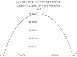
Figure 5: Evolution of $\delta\phi$ with $\eta$ through a symmetric bounce in the background.

Using the expression of $\delta\tilde{\rho}$ from Eq. (50) we can write the above equation as

$$\delta\phi^{\prime\prime}-\nabla^{2}\phi+2\tilde{\Phi}\tilde{a}^{2}V_{,\phi}+\sqrt{\frac{\kappa}{6}}(1-3c_{s}^{2})\Big{(}-\phi^{\prime 2}-2\tilde{a}^{2}\tilde{\rho}+\frac{6\tilde{\mathcal{H}}^{2}}{\kappa}\Big{)}\tilde{\Phi}\\ -2\sqrt{\frac{\kappa}{6}}(1-3c_{s}^{2})\frac{\nabla^{2}\tilde{\Phi}}{\kappa}-\left[4\phi^{\prime}-\sqrt{\frac{\kappa}{6}}(1-3c_{s}^{2})\frac{6\tilde{\mathcal{H}}^{2}}{\kappa}\right]\tilde{\Phi}^{\prime}\\ +\left[V_{,\phi\phi}+\sqrt{\frac{\kappa}{6}}(1-3c_{s}^{2})V_{,\phi}\right]\tilde{a}^{2}\delta\phi+\left[2\tilde{\mathcal{H}}+\sqrt{\frac{\kappa}{6}}(1-3c_{s}^{2})\phi^{\prime}\right]\delta\phi^{\prime}=0\,.$$ (59)

One can now solve solve Eq. (59) and Eq. (3.2) simultaneously and obtain the evolution of $\tilde{\Phi}$ and $\delta\phi$. These are the general results related to evolution of scalar metric perturbations in the longitudinal gauge worked out in the the Einstein frame which are appropriate for early universe cosmological processes as bounce. Previous authors have worked the Einstein frame perturbation equations in the synchronous gauge [32] to study the problem of structure formation in the late time universe. The results obtained in the cited work cannot in general be applied to study the problem of scalar metric perturbation evolution through a non-singular bounce and to our knowledge the appropriate longitudinal gauge results for scalar perturbation growth which we present in this paper are reported for the first time. Next we will apply the formalism in the case of a background exponential bounce. For the particular $f(R)$ model as chosen in Eq. (37) the scalar field potential $V(\phi)$ is given by:

$$V(\phi)=\frac{1}{2\kappa\alpha}\Big{(}\sqrt{\frac{2\kappa}{3}}\phi-1\Big{)}e^{-\sqrt{\frac{2\kappa}{3}}\phi}\,,$$ (60)

where $\alpha=10^{12}$. The above equations are important results reported for the first time in this paper.

3.2.1 Using the Einstein frame to model symmetric bounces in the Jordan frame

We can choose the conditions in the Einstein frame variables in such a way so that the dynamics produces a symmetric bounce in the Jordan frame. We will choose the conditions in the Einstein frame so that we can reproduce the results of the symmetric bounce in the Jordan frame as presented in the previous subsection, modulo some small numerical error which arises in the program to convert the result from Einstein frame to Jordan frame. In the Einstein frame we choose $\phi(0)=0.1$, $\phi^{\prime}(0)=0$ for the symmetric bounce background. For the perturbations we use $\tilde{\Phi}(0)=0.00015$, $\tilde{\Phi}^{\prime}(0)=0$, $\delta\phi(0)=.00002$ and $\delta\phi^{\prime}(0)=0$. The above set of values are not chosen randomly, they are chosen in such a way such that they reproduce the analogous conditions at $\eta=0$ imposed in Jordan frame perturbation calculations for the symmetric bounce, presented in the previous subsection. The background cosmological evolution is guided by the equations given at the last part of subsection 2.1. The background evolution was specified in terms of coordinate time in the Einstein frame and we use the same equations to produce the background dynamics. After the background dynamics is done in coordinate time we map the results to conformal time so that the background calculation matches with perturbation dynamics results presented in this subsection. Fig. 5 and Fig. 5 shows the evolution of $\tilde{\Phi}$ and $\delta\phi$ in the Einstein frame for a symmetric cosmological bounce in the background Jordan frame. One can now use the relations given in Eq. (40) to convert the perturbations from the Einstein frame to the Jordan frame. We expect that the results so obtained will closely match with the results obtained by the perturbation dynamics calculations done in the Jordan frame, plotted in blue in Fig. 7 and Fig. 7.

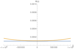
Figure 6: Evolution of $\Phi$ with $\eta$ through symmetric bounce. The blue curve represents Jordan frame result and the orange curve represents the result obtained from the Einstein frame. The details regarding the plots are given in text.

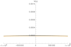
Figure 7: Evolution of $\Psi$ with $\eta$ through symmetric bounce. The blue curve represents Jordan frame result and the orange curve represents the result obtained from the Einstein frame. The details regarding the plots are given in text.

The present results are plotted in orange, in Fig. 7 and Fig. 7. We see that our results do match to a great extent, the slight mismatch results from the numerical techniques utilized in calculating the background and perturbation dynamics in the two separate frames.

3.2.2 Using the Einstein frame to model asymmetric bounces in the Jordan frame

If we consider an asymmetric bounce, we see that the nature of the scalar perturbations calculated from the two frames do not match with each other. This fact was partially noted in Ref. [13], in the present article we fully specify the gravity of the situation. At first we point out the most important difference between perturbation dynamics for the symmetric and asymmetric bounce case. In the case of an asymmetric bounce in the Jordan frame we can smoothly plot the perturbations $\Phi$, $\Psi$ in the Jordan frame as shown in Fig. 3 and Fig. 3 or $\tilde{\Phi}$, $\delta\phi$ in the Einstein frame as shown in Fig. 9 and Fig. 9. In this paper all the calculations of the perturbation dynamics is done for the Fourier mode $k=10^{-10}$. The asymmetric bounce in the Jordan frame can be obtained from an Einstein frame cosmology where $\phi(0)=0.1$ and $\phi^{\prime}(0)=10^{-8}$. These values corresponds to the values for $\cal{H}^{\prime}$ and $\cal{H}^{\prime\prime}$ applied in the Jordan frame to produce an asymmetric bounce. To plot the perturbations in the Einstein frame we have used the conditions $\tilde{\Phi}(-10^{6})=0.8,\tilde{\Phi}^{\prime}(-10^{6})=0$ and $\delta\phi(-10^{6})=0.05,\delta\phi^{\prime}(-10^{6})=0$. These values match with the analogous conditions used to plot the scalar perturbations in the case of an asymmetric bounce in the Jordan frame as shown in Fig. 3 and Fig. 3. In the Einstein frame $\tilde{\Phi}$ becomes marginally non-perturbative after for $\eta>0$ but the actual Jordan frame scalar perturbations remain perturbative within the time period of our interest. The marginal non-perturbative behavior in the Einstein frame do not posit any cosmological problem as far as the bounce in the Jordan frame is considered. The interesting feature of the asymmetric bounce appears when one tries to calculate the Jordan frame perturbation evolution using the Einstein frame results via the use of the relations in Eq. (40). Using the relations in Eq. (40) one obtains the Jordan frame results shown in Fig. 11 and Fig. 11. The results do not match with the expected result as obtained in Fig. 3 and Fig. 3. The transformation from the Einstein frame to the Jordan frame produces unavoidable singularities. The singularities arise in the case of an asymmetric bounce due to the reason that

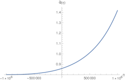
Figure 8: Evolution of $\tilde{\Phi}$ with $\eta$, in the case of an asymmetric bounce in Jordan frame, calculated directly in Einstein frame.

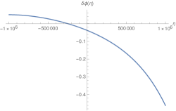
Figure 9: Evolution of $\delta{\phi}$ with $\eta$, in the case of an asymmetric bounce in Jordan frame, calculated directly in Einstein frame.

$F^{\prime}=0$ for some $\eta\neq 0$ in the time period of our interest, making the relations in Eq. (40) singular. For symmetric bounces one has $F^{\prime}(0)=a^{\prime}(0)=\tilde{\Phi}(0)=0$ and the singularity disappears in the $\eta\to 0$ limit in Eq. (40) as both the numerator and denominator tends to vanish at the same time instant. The point was partially discussed in [13]. In the present case the singularities lie near $\eta=0$ and so the Jordan frame potentials blow up near $\eta=0$ when we apply the transformations in Eq. (40) to the Einstein frame results. If the conditions used to plot the perturbations were applied at $\eta=0$ (in both the frames) then the blowing up of the potentials near $\eta=0$ distorts the values of $\Phi$ and $\Psi$ obtained far from $\eta=0$. In this case it is better to use initial conditions at $\eta=-10^{6}$, which is much further from the singularities encountered in the transformations. Before we finish this discussion we must point out that the singularities shown in the perturbation evolutions in the asymmetric case are not real singularities but an artefact of using a conformal frame which is not suitable to tackle asymmetric bounces. As a consequence our results show that the Einstein frame can be used to calculate most of the properties of a symmetric cosmological bounce in the Jordan frame including the scalar perturbation evolution. In this case the Einstein frame actually serves as an auxiliary conformal frame where the calculations can be done and the results can be converted back to the Jordan frame. On the other hand for an asymmetric bounce the Einstein frame can act as a true auxiliary frame for the background evolution but fails to reproduce the scalar perturbation dynamics in the Jordan frame. This fact is of paramount importance showing that the Jordan frame is the natural choice for scalar metric perturbation dynamics.

Figure 10: Evolution of $\Phi$ with $\eta$ through an asymmetric bounce in the Jordan frame obtained from the results in the Einstein frame.

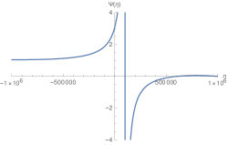
Figure 11: Evolution of $\Psi$ with $\eta$ through an asymmetric bounce in the Jordan frame obtained from the results in the Einstein frame.

3.2.3 Evolution of velocity potential in both the frames

We omitted the equation involving fluid velocity potential in the Jordan frame as the potential can be calculated from the Einstein frame itself. After showing that the scalar perturbations can be correctly calculated from the Einstein frame we directly use the Einstein frame to predict the nature of the fluid velocity potential in the Jordan frame. In the Einstein frame Eq. (52) can be used to predict the evolution of the velocity potential $\tilde{U}$. Once the evolution $\tilde{U}$ is known one can convert the result to the Jordan frame to opine on the behavior of $U$. We have $\tilde{T}^{\mu}_{\nu}=T^{\mu}_{\nu}/F^{2}$ and consequently

$$\delta\tilde{T}^{0}_{i}=\frac{\delta T^{0}_{i}}{F^{2}}-2\frac{\delta T^{0}_{i}}{F^{3}}\,.$$

As $T^{0}_{i}=0$ and the form of $\delta\tilde{T}^{0}_{i}$ (or $\delta T^{0}_{i}$) can be obtained from the form of Eq. (45) we can write

$$(\tilde{\rho}+\tilde{P})\tilde{a}^{-1}\partial_{i}\tilde{U}=\frac{(\rho+P)a^{-1}\partial_{i}U}{F^{2}}\,,$$

which yields

$$\tilde{U}=\sqrt{F}U\,.$$ (61)

The above equation shows how the velocity potentials in the two conformal frames are related to each other. The plots of the velocity potentials, when $k=10^{-10}$, for a symmetric bounce in the background is shown in Fig. 12. The blue curve represents the Jordan frame result and the orange one represents the result obtained from the Einstein frame. The results reasonably match with each other.

4 Vector perturbations in $f(R)$ cosmology

In this section we will specialize on vector metric perturbations and try to see how these perturbations evolve in $f(R)$ cosmology. In GR based bouncing models of cosmology the metric vector perturbation is bound to grow in the contracting phase of the universe [26]. But such a behavior is not in general true in $f(R)$ bouncing models as we will see below. The behavior of vector perturbations in $f(R)$ cosmology is modulated by the behavior of $F(R)$ which can keep the vector perturbations under tight control.

In the Jordan frame the metric is written as

$$g_{\mu\nu}=a^{2}(\eta)\left[\begin{array}[]{c|c}-1&S_{i}\\ \hline\cr S_{i}&\delta_{ij}-Q_{i,j}-Q_{j,i}\end{array}\right]\,,$$

and

$$g^{\mu\nu}=\frac{1}{a^{2}(\eta)}\left[\begin{array}[]{c|c}-1&S^{i}\\ \hline\cr S^{i}&\delta^{ij}+Q^{i,j}+Q^{j,i}\end{array}\right]\,,$$

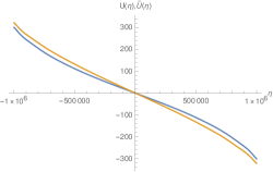
Figure 12: Evolution of fluid velocity potential $U$ and $\tilde{U}$ for a symmetric bounce in the Jordan frame. The blue curve represents the Jordan frame result and the orange curve represents the result obtained from the Einstein frame.

where $S^{i}$ and $Q^{i}$ ate 3-vectors satisfying the constraint $S^{i}_{\,\,,i}=Q^{i}_{\,\,,i}=0$. The metric in the Einstein frame is given in an identical way except that $\tilde{a}$, $\tilde{S_{i}}$ and $\tilde{Q_{i,j}}$ appear instead of $a$, $S_{i}$ and $Q_{i,j}$. More over the metric perturbations remain the same in both the conformal frames. In the Jordan frame the relevant quantities calculated from the metric given above are:

$$R_{00}=-3\mathcal{H}^{\prime}\,,\,\,\,\,\,R_{0i}=(\mathcal{H}^{\prime}+2\mathcal{H}^{2})S_{i}-\frac{1}{2}\nabla S_{i}\,,$$ (62)

where $\nabla\equiv\partial_{j}\partial^{j}$, and

$$R_{ij}=(\mathcal{H}^{\prime}+2\mathcal{H}^{2})\delta_{ij}-\frac{1}{2}(S^{\prime}_{i,j}+S^{\prime}_{j,i})-\mathcal{H}(S_{i,j}+S_{j,i})\\ -(\mathcal{H}^{\prime}+2\mathcal{H}^{2})(Q_{i,j}+Q_{j,i})-\mathcal{H}(Q^{\prime}_{i,j}+Q^{\prime}_{j,i})-\frac{1}{2}(Q^{\prime\prime}_{i,j}+Q^{\prime\prime}_{j,i})\,.$$ (63)

The Ricci tensor remains unchanged:

$$R=6\frac{(\mathcal{\dot{H}}+\mathcal{H}^{2})}{a^{2}}\,,$$ (64)

as $\delta R=0$. The perturbed Einstein tensor components are

$$\delta G^{0}_{0}=0\,,\,\,\,\,\delta G^{0}_{i}=\frac{1}{2a^{2}}\nabla S_{i}\,,$$ (65)

and

$$\delta G^{i}_{j}=-\frac{1}{2a^{2}}(S^{\prime i}_{\,\,\,,j}+S^{\prime\,\,i}_{j,})-\frac{\mathcal{H}(S^{i}_{\,\,,j}+S^{\,\,\,i}_{j,})}{a^{2}}-\frac{1}{2a^{2}}(Q^{\prime\prime i}_{\,\,\,\,\,\,,j}+Q^{\prime\prime\,\,i}_{j,})-\frac{\mathcal{H}(Q^{\prime i}_{\,\,\,,j}+Q^{\prime\,\,i}_{j,})}{a^{2}}\,,$$ (66)

where in our convention, $G_{\mu\nu}=R_{\mu\nu}-(1/2)g_{\mu\nu}R$, and, $\delta G^{\mu}_{\nu}=\delta(g^{\mu\alpha}G_{\alpha\nu})=\delta g^{\mu\alpha}G_{\alpha\nu}+g^{\mu\alpha}\delta G_{\alpha\nu}\,.$ The field equation in $f(R)$ theory is [24]:

$$G_{\mu\nu}=\frac{\kappa T_{\mu\nu}}{F(R)}+\frac{g_{\mu\nu}[f(R)-RF(R)]}{2F(R)}+\frac{D_{\mu}D_{\nu}F(R)-g_{\mu\nu}\Box F(R)}{F(R)}\,,$$ (67)

where $D_{\mu}A^{\nu}\equiv\partial_{\mu}A^{\nu}+\Gamma^{\nu}_{\mu\lambda}A^{\lambda}$ represents a covariant derivative of a contravariant 4-vector $A^{\mu}$ and $\Box\equiv g^{\mu\nu}D_{\mu}D_{\nu}$. Perturbing the above field equation one obtains

$$\delta G^{\mu}_{\nu} = \frac{\kappa\delta T^{\mu}_{\nu}}{F}-\frac{\kappa T^{\mu}_{\nu}F_{R}\delta R}{F^{2}}-\frac{\delta^{\mu}_{\nu}fF_{R}\delta R}{2F^{2}}-\frac{\left[D^{\mu}D_{\nu}F-\delta^{\mu}_{\nu}\Box F\right]F_{R}\delta R}{F^{2}(R)}$$ (68)

$$+ \frac{1}{F}\left[\delta g^{\mu\alpha}({\partial_{\alpha}\partial_{\nu}F-\Gamma^{\lambda}_{\alpha\nu}\partial_{\lambda}F})+g^{\mu\alpha}\left({\partial_{\alpha}\partial_{\nu}(F_{R}\delta R)-\delta\Gamma^{\lambda}_{\alpha\nu}\partial_{\lambda}F-\Gamma^{\lambda}_{\alpha\nu}\partial_{\lambda}(F_{R}\delta R)}\right)\right.$$

$$- \delta^{\mu}_{\nu}(\partial^{\lambda}\partial_{\lambda}(F_{R}\delta R)+\delta\Gamma^{\lambda}_{\rho\lambda}g^{\rho\kappa}(\partial_{\kappa}F)+\Gamma^{\lambda}_{\rho\lambda}\delta g^{\rho\kappa}(\partial_{\kappa}F)+\Gamma^{\lambda}_{\rho\lambda}g^{\rho\kappa}\partial_{\kappa}(F_{R}\delta R))]\,.$$

For further progress we require the perturbed fluid energy-momentum tensor in the Jordan frame, whose background value is specified in Eq. (8). In our convention we specify $u_{\mu}=-a(1,v_{i})$ where the scale-factor is expressed in conformal time and $\delta u_{i}\equiv-av_{i}$. In such a case one can easily see that $u^{\mu}=a^{-1}(1,-S^{i}-v^{i})$. By perturbing Eq. (8) one gets the non-zero components of $T^{\mu}_{\nu}$ in the absence of any anisotropic stress:

$$\delta T^{0}_{i}=-(\rho+P)v_{i}\,,\,\,\,\,\delta T^{i}_{0}=(\rho+P)(S^{i}+v^{i})\,,$$ (69)

where $\rho$ and $P$ are the background values of the thermodynamic variables. From the above set of equations one can write the dynamical equations for the perturbations as

$$\frac{1}{2a^{2}}\nabla P^{i} =-\frac{\kappa}{F}(\rho+P)v^{i}\,,$$ (70)

$$\frac{1}{2a^{2}}\partial_{\eta}\left[a^{2}(P^{i}_{\,\,,j}+P^{\,\,\,i}_{j,})\right] =-\frac{F^{\prime}}{2F}(P^{i}_{\,\,,j}+P^{\,\,\,i}_{j,})\,,$$ (71)

where

$$S^{i}+Q^{\prime i}\equiv P^{i}$$ (72)

is a gauge-invariant quantity. Henceforth we will work in the Newtonian gauge where $Q^{i}=0$. One can easily check that in the limit when $f(R)=R$ the above equations become identical to the equations for vector perturbations obtained in [26].

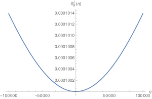
Figure 13: Evolution of vector perturbation $S^{i}_{k}$ with $\eta$ through symmetric bounce, where $S^{i}_{k}(0)=0.0001$.

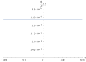
Figure 14: Evolution of velocity perturbation $v^{i}_{k}$ with $\eta$ through symmetric bounce. $S^{i}_{k}(0)$’s are the same as in the previous plot.

In the Newtonian gauge the solutions of the above equations, in the Fourier space where the subscript $k$ specifies the $k$th mode, are

$$v^{i}_{k}=\frac{k^{2}F}{2a^{2}\kappa(\rho+P)}S^{i}_{k}$$ (73)

and

$$S^{i}_{k}=\frac{C^{i}_{k}}{a^{2}F}$$ (74)

where $C^{i}_{k}$ is a constant 3-vector. Combining the above equations we get an expression for the Fourier mode of velocity perturbation as:

$$v^{i}_{k}\sim\frac{k^{2}C^{i}_{k}}{a^{1-3\omega}}\,.$$ (75)

In GR, in contracting phase of the universe, the vector metric perturbation increases as the scale-factor decreases. This growth of perturbations could pose a fundamental threat to the validity of perturbation theory. But, in $f(R)$ theory, the evolution of vector perturbation depends on the term $a^{2}F(R)$. The behavior of $F(R)$ in general affects the evolution of the vector perturbations in metric $f(R)$ cosmology.

In this paper we work with exponential gravity where the form of $f(R)$ is given in Eq. (37) where $\alpha=10^{12}$. The metric perturbation $S^{i}_{k}$ and velocity perturbation $v^{i}_{k}$ for $k=10^{-10}$, for a radiation dominated universe where $\omega=1/3$, have been plotted for a symmetric cosmological bounce in the background in Fig. 14 and Fig. 14. The conditions used for the background evolution for the symmetric bounce remains the same as specified in subsection 3.1. The plots clearly show that in $f(R)$ cosmology the vector perturbations remains practically the same through the non-singular bounce. More over the metric vector perturbation slightly diminishes during the contracting phase where as in GR the vector perturbation only increases during the contracting phase. Consequently $f(R)$ cosmology can moderate the growth of vector perturbations, a fact perhaps noted for the first time in this paper.

In the Einstein frame analysis of vector perturbations, the field equation is:

$$\tilde{R}^{\mu}_{\nu}-\frac{1}{2}\delta^{\mu}_{\nu}\tilde{R}=\kappa(\tilde{T}^{\mu}_{\nu}+S^{\mu}_{\nu})\,.$$ (76)

In the Einstein frame the effective energy-momentum tensor is $\tilde{T}^{\mu}_{\nu}+S^{\mu}_{\nu}$ where $S^{\mu}_{\nu}$ is the energy momentum tensor of a scalar field. $\tilde{T}^{\mu}_{\nu}$ is the Einstein frame counterpart of ${T}^{\mu}_{\nu}$. As the scalar field does not produce any vector perturbations only the fluid perturbations, coming from $\tilde{T}^{\mu}_{\nu}$ contribute on the right hand side of the perturbed Einstein equation. Consequently the vector perturbation equations in Einstein frame are:

$$\frac{1}{2\tilde{a}^{2}}\nabla\tilde{S}^{i}=-\kappa(\tilde{\rho}+\tilde{P})\tilde{v}^{i}\,,\,\,\,\,{\rm and}\,\,\,\,\,\,\partial_{\eta}\left[\tilde{a}^{2}(\tilde{S}^{i}_{\,\,,j}+\tilde{S}^{\,\,\,i}_{j,})\right]=0\,,$$ (77)

where we have used the results from [26]. Solving these equations we get

$$\tilde{S}^{i}_{k}=\frac{\tilde{C}^{i}_{k}}{\tilde{a}^{2}}\,,$$ (78)

which shows that $\tilde{S}^{i}_{k}=S^{i}_{k}$ when $\tilde{C}^{i}_{k}=C^{i}_{k}$. In the present case we have chosen $C^{i}_{k}=0.00015$. As in the present case the vector perturbations remain equal in both the conformal frames we do not separately present the Einstein frame result. Both the frames produce the same plots and no singularities are encountered in converting the result from Einstein frame to the Jordan frame. The present calculation shows that one can always use the Einstein frame for the calculation for vector perturbations as the calculations are much easily handled in the Einstein frame.

5 Discussion and conclusion

The present paper deals with metric perturbations in a bouncing cosmology guided by $f(R)$ theory of gravity. Scalar and vector metric perturbations during bounce in exponential gravity have been presented in this paper. The cosmological bounce takes place in the Jordan frame. The scalar metric perturbations have been calculated in the longitudinal gauge as this gauge choice remains invariant under a conformal transformation relating the Jordan frame and the Einstein frame. In the case of the vector perturbations the metric perturbations remain the same in both the frames and one can work with any gauge one wishes to. In the present paper we have worked with the Newtonian gauge. While the background evaluation of bouncing cosmologies can efficiently be calculated in the Einstein frame the perturbations on the metric and fluid variables can also be calculated in the Einstein frame where we expect the gravitational theory to be like GR with an extra scalar field. In a previous calculation the authors tried to calculate the scalar perturbations in a bouncing scenario using the Einstein frame [13] but did not take into account the fluid perturbations. Hence the earlier calculations were incomplete. In this paper the full calculation of the scalar perturbations in the Einstein frame are presented for the first time. The perturbation calculations are general although in the present case the results are applied for the particular case of a cosmological bounce in the Jordan frame. All the results presented in this paper is for an exponential $f(R)$ gravity theory which satisfies the basic stability conditions. The matter content of the universe was always assumed to be radiation fluid as these is the most general fluid which plays an important role in the very early universe.

In the present paper the critical role of the Einstein frame in aiding the calculations of Jordan frame phenomena in $f(R)$ gravity is studied in full detail. The paper establishes that the Einstein frame can be a used for the background evolutions for all the cases in the Jordan frame and also for perturbation evolution of many cases in $f(R)$ gravity except the particular case of asymmetrical bounce in the Jordan frame where one cannot transform the scalar metric perturbation back to the Jordan frame. Although the correspondence of the background cosmological evolution in the conformal frames, for $f(R)$ based cosmology, was noted much earlier [23, 29] here one must note that in [13] it was pointed out that for the case of a cosmological bounce in presence of matter, which satisfies $\rho+P\geq 0$ in the Jordan frame, there is no corresponding cosmological bounce in the conformally related Einstein frame when one works with spatially flat FLRW spacetimes. As far as cosmological bounce in flat FLRW spacetime is concerned, the Einstein frame acts like a true auxiliary frame where one can do all the calculations and then convert the results appropriately in the Jordan frame. For cosmological perturbations one can also use the Einstein frame as the auxiliary frame but as far as scalar perturbations are concerned the conformal correspondence fails for asymmetric bounces. This particular failure is not a physical problem as shown in the present paper. The perturbations evolve smoothly in both the Jordan frame calculation and Einstein frame calculation. The problem arises in the connecting formulae which connect the Jordan frame perturbations with the Einstein frame perturbation. The paper presents the calculations of perturbations separately in both the conformal frames and then connects the results to show the validity of the Einstein frame results. The nature of the variation of the fluid velocity potential in the Jordan frame is also presented in the paper.

The next part of the present paper deals with the evolution of vector perturbations during a non-singular bounce in $f(R)$ gravity. This calculation shows that for vector perturbations one can actually use the Einstein frame for all the cases and the calculations do become much easier in the Einstein frame. The vector perturbations remains the same in both the frames and no singularity appears anywhere in the description of vector perturbations from the Einstein frame. In GR based cosmological models it was shown that one expects the vector perturbations to be increasing during the contracting phase. For a singular bounce the vector perturbations can diverge during the bounce. In the present paper we have only studied non-singular bounce in exponential gravity and the results regarding the evolution of vector perturbations during such a phase are interesting. In this case the vector perturbations practically remains constant during the bouncing phase showing stability of the perturbation modes. One can expect that in the deep expansion phase of the universe this vector modes do get diluted. There has been studies on magnetic field generation in the early universe and the nature of vector perturbations, we expect the specific nature of the evolution of vector perturbations in the present case can have interesting consequences for magnetogenesis.

The question of tensor perturbation in general $f(R)$ gravity and in particular related to bouncing scenarios has not been presented in the paper. Tensor perturbations will be taken up in a future publication as there are various interesting issues related to primordial tensor perturbations which require separate and thorough investigation. The present work presupposes that the earlier universe (much before the bouncing time) and the later universe (much later than the bouncing time) were guided by a theory of gravity like GR which gets effectively modified to exponential gravity in the high curvature limit near the bounce. The change over from GR to $f(R)$ is non-trivial and will require new physics. The perturbation modes earlier and later than the bounce are expected to follow standard cosmological dynamics obtained from GR. In this process our main aim is to show how the perturbation modes evolve during the bouncing time. It is shown that the perturbation modes can solely be tackled from the accompanying, conformally connected Einstein frame for most of the cases. The perturbation modes which have been studied remain perturbative throughout the bounce, but this does not comprehensively specify that all the perturbations are stable. The vector perturbations should be stable for all initial values but it is very difficult to generalize the statement for scalar perturbations for all initial values of the perturbations. There may remain some modes with specific initial conditions which tend to become non-perturbative near the bounce. In such cases one has to bring in new physics to settle the issue of perturbative instability. While our work does not prove perturbative stability in the most general way it definitely shows how the stable perturbations evolve near the bounce.

References

- [1] A. A. Starobinsky, Phys. Lett. B 91, 99 (1980) [Phys. Lett. 91B, 99 (1980)] [Adv. Ser. Astrophys. Cosmol. 3, 130 (1987)]. doi:10.1016/0370-2693(80)90670-X
- [2] A. H. Guth and S. Y. Pi, Phys. Rev. Lett. 49, 1110 (1982). doi:10.1103/PhysRevLett.49.1110
- [3] A. Borde and A. Vilenkin, Int. J. Mod. Phys. D 5, 813 (1996) doi:10.1142/S0218271896000497 [gr-qc/9612036].
- [4] J. Martin and R. H. Brandenberger, Phys. Rev. D 63, 123501 (2001) doi:10.1103/PhysRevD.63.123501 [hep-th/0005209].
- [5] R. H. Brandenberger and J. Martin, Class. Quant. Grav. 30, 113001 (2013) doi:10.1088/0264-9381/30/11/113001 [arXiv:1211.6753 [astro-ph.CO]].
- [6] J. Martin, P. Peter, N. Pinto Neto and D. J. Schwarz, Phys. Rev. D 65, 123513 (2002) doi:10.1103/PhysRevD.65.123513 [hep-th/0112128].
- [7] J. Martin and P. Peter, Phys. Rev. D 68, 103517 (2003) doi:10.1103/PhysRevD.68.103517 [hep-th/0307077].
- [8] D. Battefeld and P. Peter, Phys. Rept. 571, 1 (2015) doi:10.1016/j.physrep.2014.12.004 [arXiv:1406.2790 [astro-ph.CO]].
- [9] M. Novello and S. E. P. Bergliaffa, Phys. Rept. 463, 127 (2008) doi:10.1016/j.physrep.2008.04.006 [arXiv:0802.1634 [astro-ph]].
- [10] Y. F. Cai, D. A. Easson and R. Brandenberger, JCAP 1208, 020 (2012) doi:10.1088/1475-7516/2012/08/020 [arXiv:1206.2382 [hep-th]].
- [11] L. R. Abramo, I. Yasuda and P. Peter, Phys. Rev. D 81, 023511 (2010) doi:10.1103/PhysRevD.81.023511 [arXiv:0910.3422 [hep-th]].
- [12] S. Carloni, P. K. S. Dunsby and D. M. Solomons, Class. Quant. Grav. 23, 1913 (2006) doi:10.1088/0264-9381/23/6/006 [gr-qc/0510130].
- [13] N. Paul, S. N. Chakrabarty and K. Bhattacharya, JCAP 1410, no. 10, 009 (2014) doi:10.1088/1475-7516/2014/10/009 [arXiv:1405.0139 [gr-qc]].
- [14] K. Bhattacharya and S. Chakrabarty, JCAP 1602, no. 02, 030 (2016) doi:10.1088/1475-7516/2016/02/030 [arXiv:1509.01835 [gr-qc]].
- [15] K. Bamba, A. N. Makarenko, A. N. Myagky, S. Nojiri and S. D. Odintsov, JCAP 1401, 008 (2014) doi:10.1088/1475-7516/2014/01/008 [arXiv:1309.3748 [hep-th]].
- [16] P. Bari, K. Bhattacharya and S. Chakraborty, Universe 4, no. 10, 105 (2018). doi:10.3390/universe4100105
- [17] R. Myrzakulov, L. Sebastiani and S. Zerbini, Int. J. Mod. Phys. D 22, 1330017 (2013) doi:10.1142/S0218271813300176 [arXiv:1302.4646 [gr-qc]].
- [18] T. Clifton, P. G. Ferreira, A. Padilla and C. Skordis, Phys. Rept. 513, 1 (2012) doi:10.1016/j.physrep.2012.01.001 [arXiv:1106.2476 [astro-ph.CO]].
- [19] K. Atazadeh and H. R. Sepangi, Int. J. Mod. Phys. D 16, 687 (2007) doi:10.1142/S0218271807009838 [gr-qc/0602028].
- [20] S. M. Carroll, V. Duvvuri, M. Trodden and M. S. Turner, Phys. Rev. D 70, 043528 (2004) doi:10.1103/PhysRevD.70.043528 [astro-ph/0306438].
- [21] S. Nojiri, S. D. Odintsov and V. K. Oikonomou, Phys. Rept. 692, 1 (2017) doi:10.1016/j.physrep.2017.06.001 [arXiv:1705.11098 [gr-qc]].
- [22] S. Nojiri and S. D. Odintsov, Phys. Rept. 505, 59 (2011) doi:10.1016/j.physrep.2011.04.001 [arXiv:1011.0544 [gr-qc]].
- [23] K. i. Maeda, Phys. Rev. D 39, 3159 (1989). doi:10.1103/PhysRevD.39.3159
- [24] T. P. Sotiriou and V. Faraoni, Rev. Mod. Phys. 82, 451 (2010) doi:10.1103/RevModPhys.82.451 [arXiv:0805.1726 [gr-qc]].
- [25] A. De Felice and S. Tsujikawa, Living Rev. Rel. 13, 3 (2010) doi:10.12942/lrr-2010-3 [arXiv:1002.4928 [gr-qc]].
- [26] T. J. Battefeld and R. Brandenberger, Phys. Rev. D 70, 121302 (2004) doi:10.1103/PhysRevD.70.121302 [hep-th/0406180].
- [27] A. Riotto, ICTP Lect. Notes Ser. 14, 317 (2003) [hep-ph/0210162].
- [28] D. Baumann, “Inflation,” arXiv:0907.5424 [hep-th].
- [29] V. F. Mukhanov, H. A. Feldman and R. H. Brandenberger, Phys. Rept. 215, 203 (1992). doi:10.1016/0370-1573(92)90044-Z
- [30] B. Xue, D. Garfinkle, F. Pretorius and P. J. Steinhardt, Phys. Rev. D 88, 083509 (2013) doi:10.1103/PhysRevD.88.083509 [arXiv:1308.3044 [gr-qc]].
- [31] J. Matsumoto, Phys. Rev. D 87, no. 10, 104002 (2013) doi:10.1103/PhysRevD.87.104002 [arXiv:1303.6828 [hep-th]].
- [32] R. Bean, D. Bernat, L. Pogosian, A. Silvestri and M. Trodden, Phys. Rev. D 75, 064020 (2007) doi:10.1103/PhysRevD.75.064020 [astro-ph/0611321].
- [33] E. V. Linder, Phys. Rev. D 80, 123528 (2009) doi:10.1103/PhysRevD.80.123528 [arXiv:0905.2962 [astro-ph.CO]].
- [34] S. D. Odintsov, D. S ez-Chill n G mez and G. S. Sharov, Eur. Phys. J. C 77, no. 12, 862 (2017) doi:10.1140/epjc/s10052-017-5419-z [arXiv:1709.06800 [gr-qc]].
- [35] K. Bamba, C. Q. Geng and C. C. Lee, JCAP 1008, 021 (2010) doi:10.1088/1475-7516/2010/08/021 [arXiv:1005.4574 [astro-ph.CO]].
- [36] J. D. Barrow and A. C. Ottewill, J. Phys. A 16, 2757 (1983). doi:10.1088/0305-4470/16/12/022