Abstract

We study the dynamics of inflation driven by an adiabatic self-gravitating medium, extending the previous works on fluid and solid inflation. Such a class of media comprises perfect fluids, zero and finite temperature solids. By using an effective field theory description, we compute the power spectrum for the scalar curvature perturbation of constant energy density hypersurface $\zeta$ and the comoving scalar curvature perturbation ${\cal R}$ in the case of slow-roll, super slow-roll and $w$-media inflation, an inflationary phase with $w$ constant in the range $-1<w<-1/3$. A similar computation is done for the tensor modes. Adiabatic media are characterized by intrinsic entropy perturbations that can give a significant contribution to the power spectrum and can be used to generate the required seed for primordial black holes. For such a media, the Weinberg theorem is typically violated and on super horizon scales neither $\zeta$ nor ${\cal R}$ are conserved and moreover $\zeta\neq{\cal R}$. Reheating becomes crucial to predict the spectrum of the imprinted primordial perturbations. We study how the difference between $\zeta$ and ${\cal R}$ during inflation gives rise to relative entropic perturbations in $\Lambda$CDM.

1 Introduction

Inflation is probably the most successful way to solve the horizon problem in cosmology and, at the same time, to give a simple explanation of the indirectly observed spectrum of primordial perturbations. In the case of single field, inflationary predictions are largely independent on the details of the reheating phase. Indeed, according to the Weinberg theorem [1, 2], irrespective of the constituents of the Universe, there is always an adiabatic mode, constant on superhorizon scales, which can be identified with the comoving curvature perturbation ${\cal R}$, or equivalent with the uniform curvature perturbation $\zeta$. When the theorem holds, ${\cal R}$ or equivalently $\zeta$ can be used to set the initial conditions for the perturbations in the thermal radiation dominated phase of the Universe. Thus, the power of the Weinberg theorem relies in the possibility of simply inflate and forget about the largely unknown period when the inflaton dominated Universe is turned into a radiation dominated one. However, going beyond single field inflation can trigger violation of the Weinberg theorem; for instance, multi-field inflation will typically produce a mixture of adiabatic and isocurvature primordial perturbations, as a result ${\cal R}$ and $\zeta$ will not be constant on super-horizon scales. In this framework, it is very useful to explore the general physical implications on symmetry grounds instead of dealing with a plethora of different models. In the case of single clock inflation, the inflaton itself can be used as a “clock” that breaks spontaneously time reparametrization invariance of general relativity (GR); the effective action description was given in [3], see also [4] for a different formulation.

More subtle violations can take place when neither ${\cal R}$ nor $\zeta$ are conserved at superhorizon scales [5, 6, 7, 8, 9]. This is the case, for instance, for fluid [10] and solid inflation [11]. In the present work, we present a general set up capable to give an effective field theory description of inflation driven by a generic adiabatic, non-dissipative medium. Such effective theory description [12, 13, 14, 15, 16, 17] is based on four scalar fields $\{\varphi^{A}\,,\;A=0,1,2,3\}$, and comprise fluid inflation and solid inflation and their generalization, namely non-barotropic fluid inflation and finite temperature solid inflation. The basic assumption is that the entropy per particle perturbation $\delta\sigma$, when present, is conserved in time. It is worth to point out that, though $\delta\sigma$ is time independent, it can give an important contribution to the power spectrum; in particular, it can be used as initial seed of perturbation for the generation of primordial black holes that could constitute a sizable amount of dark matter in our universe [18, 19, 20, 21]. The case of a constant in time $\delta\sigma$ also constitutes a simplified dynamical setup to study a generic supersolid , the most general case of a non-dissipative self-gravitating medium, which has two propagating scalar modes and one is precisely $\delta\sigma$ [17]. Indeed, in this case the entropy perturbations becomes constant at superhorizon scales in a wide range of parameters.

The outline of the paper is the following. In section 2 we briefly review the effective field theory description of adiabatic self-gravitating media. In section 3, the dynamics of ${\cal R}$ and $\zeta$ is derived in general terms, discussing possible sources of violation of the Weinberg theorem. Section 4 is devoted to study the dynamics of inflation driven by an adiabatic medium giving the general expression of ${\cal R}$ and $\zeta$ and the corresponding power spectrum; in particular the role of entropic perturbation is studied. In section 5 we give a detailed analysis of inflation for barotropic and non-barotropic fluids, zero-temperature and finite temperature solids in the following regimes of interest: slow-roll, super slow-roll and $w$-media inflation. Section 6 deals with tensor modes during inflation and the resulting tensor-scalar ratio. Section 7 is devoted to the study of the post inflationary phase that leads to a radiation dominated Universe by computing the final values of ${\cal R}$ and $\zeta$. Our conclusions are given in Section 8.

2 Self-Gravitating Media

The effective field theory (EFT) description of the dynamics of a generic non-dissipative medium can be used to systematically describes the symmetry breaking pattern of spacetime symmetry during inflation. The EFT is based on four Stuckelberg scalar fields $\varphi^{A}$, $A=0\,,1\,,\,2\,,\,3$, related to the Goldstone bosons for the spontaneous breaking of spacetime translations [13, 17]. The action is required to be invariant under shift symmetry $\varphi^{A}\rightarrow\varphi^{A}+c^{A}$. Among the set of scalar operators containing a single derivative of $\varphi^{A}$

$$\{C^{AB}=g^{\mu\nu}\partial_{\mu}\varphi^{A}\,\partial_{\nu}\varphi^{B}\;\qquad A,B=0,1,2,3\}\,,$$ (2.1)

imposing internal $SO(3)$ invariance selects 8 independent operators  that can enter in the EFT action [17, 23]

$$\begin{split}&X=C^{00},\quad Y=u^{\mu}\partial_{\mu}\varphi^{0},\quad\tau_{i}=\text{Tr}\left[\textbf{B}^{i}\right]\;\;i=1,2,3,\quad y_{n}=\text{Tr}\left(\boldsymbol{B}^{n}\cdot\boldsymbol{Z}\right)\;\;n=0,1,2,3,\\ &\left(\textbf{B}\right)^{ab}=C^{ab},\qquad Z^{ab}=C^{a0}\,C^{b0}\quad\;a=1,2,3\,;\end{split}$$ (2.2)

where we have introduced the four velocity of the medium $u^{\mu}$ such that $u^{\mu}\partial_{\mu}\varphi^{a}=0$

$$u^{\mu}=-\frac{\epsilon^{\mu\nu\alpha\beta}}{6\;b\;\sqrt{-g}}\,\epsilon_{abc}\;\partial_{\mu}\varphi^{a}\,\partial_{\nu}\varphi^{b}\,\partial_{\beta}\varphi^{c}\,,\qquad u^{2}=-1\,.$$ (2.3)

The $b$ operator is given by the following combination of $\tau_{i}$

$$b=\text{Det}(\boldsymbol{B})^{1/2}=\left(\frac{\tau_{1}^{3}-3\,\tau_{1}\,\tau_{2}+2\,\tau_{3}}{6}\right)^{1/2}\,.$$ (2.4)

The most general non-dissipative medium minimally coupled with gravity (self-gravitating) is described by the action

$$S=M_{pl}^{2}\int d^{4}x\,\sqrt{-g}\;R+\int d^{4}x\,\sqrt{-g}\,U(X,\,Y,\,\tau_{i},\,y_{n})\,.$$ (2.5)

whose energy density and isotropic pressure are given by

$$\rho=-U+Y\;U_{Y}-2\;Y^{2}\;U_{X}$$ (2.6)

$$p=U-b\;U_{b}-\frac{2}{3}\;U_{X}\;(Y^{2}+X)-\frac{2}{3}\;\sum_{n=1}^{3}\;n\;\tau_{n}\;U_{\tau_{n}}-\frac{2}{3}\,\sum_{n=0}^{3}\;(n+1)\;y_{n}\;U_{y_{n}}\,.$$ (2.7)

The entropy density $s$ can be expressed in terms of the Noether current $J^{0}_{\mu}$ of the shift symmetry of $\varphi^{0}$ as

$$s=-u^{\alpha}\,J_{\alpha}^{0}=U_{Y}-2\;Y\;U_{X}\,,$$ (2.8)

and the temperature $T$ is represented by the operator $Y$. The number density $n$ can be identified as the projection along the four-velocity of an off shell conserved current

$$n=-u_{\alpha}\,J^{\alpha}\,,\qquad J_{\alpha}=b\,u_{\alpha}\,,\qquad\nabla^{\alpha}\,J_{\alpha}=0\,.$$ (2.9)

Finally, the conservation of entropy per particle $\sigma=s/n$ along the flow lines gives

$$u^{\alpha}\nabla_{\alpha}\sigma=-\frac{2}{b}\;\nabla^{\alpha}\;\left[\;U_{X}\left(Y\,u_{\alpha}+\partial_{\alpha}\varphi^{0}\right)+\;\sum_{n=0}^{3}\;U_{y_{n}}\;{\cal C}^{0a}\;({B}^{n})^{ab}\;\partial_{\alpha}{\varphi}^{b}\right]\,.$$ (2.10)

Internal symmetries can be used to enforce some special thermodynamical and dynamical properties of the medium. The mechanical properties are obtained analysing the structure of the EMT (a full analysis is given in [16, 17]). It is useful to summarize the main features associated with the presence/absence of some of the operators in the Lagrangian which corresponds to specific internal symmetries.

• Perfect Fluids:

  • $U(b,\,Y):$ only $\{\varphi^{a}\,,\;\;a=1,2,3\}$ are present; the Lagrangian is invariant under internal volume preserving diffeomorphisms $V_{s}\text{Diff}$: $\varphi^{a}\to\Psi^{a}(\varphi^{b})$ , $\det|\partial\Psi^{a}/\partial{\varphi^{b}}|=1$, $a,b=1,2,3$.

  • $U(X):$ it is the most general Lagrangian for a perfect irrotational fluid with only $\varphi^{0}$ present.

• Superfluids $U(b,\,Y,\,X):$ invariant under transformations of $\varphi^{a}$ corresponding to $V_{s}\text{Diff}$ and $\varphi^{0}\to\varphi^{0}+f(\varphi^{a})$.

• Solids $U(Y,\,\tau_{i}):$ most general Lagrangian with only $\{\varphi^{a}\,,\;\;a=1,2,3\}$ present.

• Supersolids $U(Y,\,X,\,\tau_{i},\,y_{n})$.

The main thermodynamical characterization of the medium is based on (2.10).

• When $u^{\alpha}\nabla_{\alpha}\sigma=0$ the medium is named adiabatic.
  The conservation of $\sigma$ can be enforced by a symmetry which forbids the presence of $X$ and $y_{n}$ in the Lagrangian. This is the case for the $\varphi^{a}$-dependent shift of $\varphi^{0}$, namely

  $$\varphi^{0}\to\varphi^{0}+f(\varphi^{a})\,,\qquad a=1,2,3\,;$$ (2.11)

  where only $Y$ and $\tau_{i}$ are left invariant (and also the operator $b$). In such a way we can identify as adiabatic media: finite temperature non-barotropoic perfect fluids described by the Lagrangian $U(b,\,Y)$ and finite temperature solids described by $U(Y,\,\tau_{i})$.

• When $\sigma=0$ the medium is named isentropic.
  Isentropic media are characterized by the absence of $Y$ and $X$ in the Lagrangian. Such a class of media includes perfect fluids $U(b)$, solids $U(\tau_{n})$ and some specific superfluids and supersolids see  [17].

Notice that in a FRW background, if $\sigma$ is constant in time, it can have a non-trivial spatial distribution.
In the rest of this paper we will only consider adiabatic media; the general case with a dynamical $\sigma$ will be studied elsewhere [22].
In flat spacetime, the dynamics of an adiabatic medium can be found by studying the fluctuations around a rotational invariant configuration by taking

$$g_{\mu\nu}=\eta_{\mu\nu},\qquad\varphi^{0}=t+\pi_{0}\,,\qquad\varphi^{i}=x^{i}+\partial^{i}\pi_{L}+\pi_{T}^{i}\,,\qquad\partial_{i}\pi_{T}^{i}=0\,.$$ (2.12)

At the quadratic level we have

$$\begin{split}{\cal S}^{(2)}&=M_{\text{Pl}}^{2}\int d^{4}x\Big{[}\frac{(\bar{\rho}+\bar{p})}{2}\,\partial_{t}\pi_{L}\,\Delta\,\partial_{t}\pi_{L}+\left(M_{3}-M_{2}\right)\pi_{L}\Delta^{2}\pi_{L}+M_{0}\,{\pi_{0}^{\prime}}^{2}+2\,M_{4}\,\pi_{0}^{\prime}\Delta\pi_{l}\\ &+\frac{(\bar{\rho}+\bar{p})}{2}\,\partial_{t}\pi_{T}^{i}\,\partial_{t}\pi_{T}^{i}-\frac{M_{2}}{2}\pi_{T}^{i}\,\Delta\pi_{T}^{i}\Big{]}\,;\end{split}$$ (2.13)

where $\bar{\rho}$ and $\bar{p}$ are the background values of the energy density and pressure (constant in space and time) while $\Delta=\delta_{ij}\partial_{i}\partial_{j}$; finally the time derivative of a function $f$ is denoted by $f^{\prime}$. We have also introduced the mass parameters $\{M_{A}\,;A=0,1,2,3,4\}$ which characterize the quadratic action of a self-gravitating medium; their definition in terms of the derivative of $U$ is given in appendix A.1. The main feature of the symmetry (2.11) is that the temporal Stuckelberg field $\pi_{0}$ enters in the quadratic action only through its time derivative and one can make a field redefinition by setting $\pi_{0}^{\prime}=\Pi$, then $\Pi$ can be integrated out from the quadratic action by using its algebraic equation of motion; namely

$$\Pi=c_{b}^{2}\,\Delta\pi_{L}+F(\vec{x})\,\,,$$ (2.14)

where $F(\vec{x})$ is an arbitrary function of the spatial coordinates $x^{i}$. One then gets 

$${\cal S}^{(2)}=M_{\text{Pl}}^{2}\int d^{4}x\,(\bar{\rho}+\bar{p})\,\Big{[}\frac{1}{2}\partial_{t}\pi_{L}\Delta\partial_{t}\pi_{L}-\frac{c_{L}^{2}\,}{2}\pi_{L}\Delta^{2}\pi_{L}+\frac{1}{2}\partial_{t}\pi_{T}^{i}\partial_{t}\pi_{T}^{i}-\frac{M_{2}}{2\,(\bar{\rho}+\bar{p})}\pi_{T}^{i}\Delta\pi_{T}^{i}\Big{]}\,;$$ (2.15)

with

$$c_{b}^{2}=-\frac{M_{4}}{M_{0}}\,.$$ (2.16)

There the longitudinal modes propagate with velocity

$$c_{L}^{2}=\frac{2\,M_{\text{Pl}}^{2}\left[M_{4}^{2}+M_{0}\left(M_{2}-M_{3}\right)\right]}{M_{0}\,(\bar{\rho}+\bar{p})}\equiv c_{s}^{2}+\frac{4}{3}\,c_{T}^{2}\,,$$ (2.17)

where

$$c_{s}^{2}=\frac{2\,M_{\text{Pl}}^{2}\left[3M_{4}^{2}+M_{0}\left(M_{2}-3M_{3}\right)\right]}{3\,M_{0}\,(p+\rho)}$$ (2.18)

is the adiabatic sound speed, while

$$c_{T}^{2}=\frac{M_{\text{Pl}}^{2}\,M_{2}}{(\bar{\rho}+\bar{p})}$$ (2.19)

is the propagation speed of the transverse modes.

The case $M_{0}=0$  is special and corresponds to an enhanced symmetry which turns the adiabatic medium into an isentropic one [17]. The quadratic action can be obtained by simply setting $\pi_{0}^{\prime}=0$ in (2.15); the longitudinal modes propagate with velocity $c_{L}^{2}$ where the adiabatic sound speed $c_{s}^{2}$ this time is given by

$$c_{s}^{2}=\frac{2\,M_{\text{Pl}}^{2}(M_{2}-3\,M_{3})}{9\,(\bar{\rho}+\bar{p})}\,.$$ (2.20)

Stability in flat spacetime requires that

$$(\bar{\rho}+\bar{p})>0\,\qquad M_{3}>M_{2}\,,\qquad M_{2}>0\,,$$ (2.21)

or equivalently $(\bar{\rho}+\bar{p})>0$ and $c_{L}^{2}>0$, $c_{T}^{2}>0$ which is the null energy condition augmented by the positivity relations for the mass parameters entering in the dynamics of the fluctuations of the medium, see [16, 17]. Notice that when the operator $X=g^{\mu\nu}\partial_{\mu}\varphi^{0}\partial_{\nu}\varphi^{0}$ is present in the Lagrangian, $\pi_{0}$ is a genuine propagating mode (at the quadratic level this happens when $M_{1}\neq 0$) and the medium is non longer adiabatic and it will feature two scalars and two vectors propagating modes.

3 $\zeta$ and ${\cal R}$ Evolution

The scalar part of the perturbed metric in the conformal Newtonian gauge takes the form

$$g_{00}=a^{2}(-1+2\,\psi)\,,\qquad g_{0i}=0\,,\qquad g_{ij}=a^{2}(1+2\,\phi)\delta_{ij}\,,$$ (3.1)

$$\varphi^{0}=\bar{\varphi}(t)+\pi_{0}\,,\qquad\varphi^{i}=x^{i}+\partial_{i}\pi_{L}\,.$$ (3.2)

We employ conformal time and, as before, time derivative of a function $f$ is denoted by $f^{\prime}$. A generic medium will sport both density and entropy perturbations, a general discussion can be found in [16, 17], the relation with massive gravity is discussed in [23, 24]. For our purpose, we just need to consider perturbations of adiabatic media. By using the EFT for isentropic media, one can write in a closed form the equations governing the dynamics of the comoving and uniform curvature gauge invariant perturbations defined by

$${\cal R}=-\phi-{\cal H}\,v,\qquad\qquad\zeta=-\phi-\frac{\delta\rho}{3(\bar{\rho}+\bar{p})}\,;$$ (3.3)

where $v$ is the scalar part of the medium’s velocity, $\bar{p}$ and $\bar{\rho}$ are the background values while ${\cal H}=a^{\prime}/a$ is the conformal Hubble parameter. The dynamics of perturbation is encoded in very few parameters, namely the equation of state $w=\bar{p}/\bar{\rho}$, the various sound velocities defined in (2.16), (2.18), (2.19) and (2.17). In general, the pressure perturbation can be written as

$$\delta p=c_{s}^{2}\,\delta\rho+\Gamma\,;$$ (3.4)

which define the non-adiabatic contribution $\Gamma$. The scalar perturbations ${\cal R}$, $\zeta$, the scalar anisotropic stress $\Xi$ and $\Gamma$ are related by

$$\zeta=\mathcal{R}+\frac{a^{2}\,\Gamma}{18\,M_{\text{Pl}}^{2}\,(w+1)\,\mathcal{H}^{2}\,c_{s}^{2}}+\frac{k^{2}\,\Xi}{27\,(w+1)\,\mathcal{H}^{2}\,c_{s}^{2}}-\frac{\mathcal{R}^{\prime}}{3\,\mathcal{H}\,c_{s}^{2}}\,,$$ (3.5)

By using the EFT for the medium, one can derive the expression of the energy density and pressure perturbations $\delta\rho$ and $\delta p$, the scalar part $\Xi$ of the anisotropic stress and the perturbation $\delta\sigma$ of the entropy per particle in terms of the Stuckelberg fields [17]; namely

$${\delta\rho}=-\frac{6\,M_{\text{Pl}}^{2}\,\mathcal{H}^{2}}{a^{2}}\left(3\,\phi+k^{2}\,\pi_{L}\right)\;(1+w)+\frac{\bar{\varphi}^{\prime}}{a^{4}}\;\delta\sigma\,;$$ (3.6)

$$\delta p=-\frac{6\,M_{\text{Pl}}^{2}\,\mathcal{H}^{2}}{a^{2}}\,c_{s}^{2}\;\left(3\,\phi+k^{2}\,\pi_{L}\right)\;(1+w)+\frac{c_{b}^{2}\;\bar{\varphi}^{\prime}}{a^{4}}\;\delta\sigma\,;$$ (3.7)

$$\Xi=2\,M_{pl}^{2}\,(\phi-\psi)=-\frac{2\,M_{pl}^{2}\,M_{2}}{a^{2}}\,\pi_{L}\,;$$ (3.8)

$$\delta\sigma=2\,M_{\text{Pl}}^{2}\,\frac{M_{0}}{\bar{\varphi}^{\prime}}\,\left[\psi+\frac{\pi_{0}^{\prime}}{\bar{\varphi}^{\prime}}+c_{b}^{2}\left(3\,\phi+k^{2}\,\pi_{L}\right)\right]\,.$$ (3.9)

By comparison of (3.6), (3.9) and (3.4) we deduce that

$$\Gamma=\frac{\bar{\varphi}^{\prime}\,\left(c_{b}^{2}-c_{s}^{2}\right)}{a^{4}}\;\delta\sigma\,.$$ (3.10)

The dynamics of $\sigma$ is such that

$$\delta\sigma^{\prime}=\frac{k^{2}\,M_{\text{Pl}}^{2}\,M_{1}\,\left(\pi_{0}-\pi_{L}^{\prime}\,\phi^{\prime}\right)}{\phi^{\prime}{}^{2}}\,;$$ (3.11)

in agreement with the fact that when the medium is adiabatic, as enforced by (2.11), then $M_{1}=0$ and $\sigma^{\prime}=0$. Though $\delta\sigma$ does not depend on time, in general it will be a nontrivial function $\delta\sigma(\vec{x})$ of the spatial coordinates $\vec{x}$ or of the comoving momentum $\vec{k}$ in Fourier space. $\delta\sigma$ becomes a propagating mode when the symmetry (2.11) is not enforced and the medium is not adiabatic anymore. We stress that, even in the general case, where $\delta\sigma$ is propagating, the entropy perturbations are constant on superhorizon scales under mild assumptions, see appendix C.
The uniform curvature perturbation $\zeta$ can be expressed in terms of $\delta\sigma$ and the longitudinal phonon mode $\pi_{L}$

$$\zeta=\frac{k^{2}}{3}\,\pi_{L}-\frac{\bar{\varphi}^{\prime}}{3\,a^{4}\,(\bar{\rho}+\bar{p})}\,\delta\sigma\,.$$ (3.12)

Then by using the expressions for the anisotropic stress (3.8) and for $\delta\sigma$ (3.9) and (3.10) given by EFT, one gets the following relation among uniform and comoving curvature perturbations and entropy per particle perturbation

$$\frac{\bar{\varphi}^{\prime}\,\left(c_{L}^{2}-c_{b}^{2}\right)}{18\,a^{2}\,M_{\text{Pl}}^{2}\,(w+1)\,\mathcal{H}^{2}\,c_{L}^{2}}\,\delta\sigma-\mathcal{R}\,\frac{c_{s}^{2}}{c_{L}^{2}}+\frac{\mathcal{R}^{\prime}}{3\,\mathcal{H}\,c_{L}^{2}}+\zeta=0\,.$$ (3.13)

The perturbed Einstein equations lead to the following dynamical equation for ${\cal R}$

$$\left({\cal R}^{\prime}\,L_{\cal R}\right)^{\prime}+m_{\cal R}^{2}\,{\cal R}+A_{\sigma}\,\delta\sigma=0\,,\qquad\qquad L_{\cal R}=\frac{a^{2}\,(w+1)}{c_{L}^{2}}\,;$$ (3.14)

where

$$\begin{split}&m_{\cal R}^{2}=\frac{a^{2}\,(1+w)}{c_{L}^{4}}\left\{k^{2}\,c_{L}^{4}+2\,\mathcal{H}\,c_{L}^{2}\left[3\,(w+1)\,\mathcal{H}\,c_{T}^{2}+2\,c_{T}^{2}{}^{\prime}\right]-4\,\mathcal{H}\,c_{T}^{2}\,c_{L}^{2}{}^{\prime}\right\}\,;\\ &A_{\sigma}=\frac{\bar{\varphi}^{\prime}}{M_{pl}^{2}}\left[\frac{(w+1)\left(c_{L}^{2}-c_{b}^{2}\right)+2\,c_{b}^{2}\left(c_{b}^{2}-c_{s}^{2}\right)}{4\,c_{L}^{2}}-\frac{c_{b}^{2}{}^{\prime}}{6\,\mathcal{H}\,c_{L}^{2}}+\frac{c_{b}^{2}\,c_{L}^{2}{}^{\prime}}{6\,\mathcal{H}\,c_{L}^{4}}\right]\,.\end{split}$$ (3.15)

As discussed in section 2, $c_{T}$, $c_{L}$ and $c_{b}$ are functions of the mass parameters $\{M_{A}\,,\;A=0,1,2,3,4\}$ which are expressed in terms of first and second derivatives of the Lagrangian describing the medium, see appendix A and [17]. A similar equation for $\zeta$ can be obtained by using (3.5) and it is given in appendix B.
By using the field redefinition ${\cal R}_{c}=L_{\cal R}^{\frac{1}{2}}\;{\cal R}$, the evolution eq. (3.14) for ${\cal R}$  can be recast in the following canonical form

$${\cal R}_{c}^{\prime\prime}+m_{{\cal R}_{c}}^{2}\,{\cal R}_{c}+\frac{A_{\sigma}}{L_{\cal R}^{1/2}}\,\delta\sigma=0\,,\qquad\qquad m_{{\cal R}_{c}}^{2}=\frac{m_{\cal R}^{2}}{L_{\cal R}}-\frac{L_{\cal R}^{\prime\prime}}{2\,L_{\cal R}}+\frac{L_{\cal R}^{\prime}{}^{2}}{4\,L_{\cal R}^{2}}\,.$$ (3.16)

The above equation can be used to study the violation of the Weinberg theorem; indeed when $\delta\sigma=0$ (isentropic medium), the curvature perturbations ${\cal R}$ or $\zeta$ can grow at superhorizon scales if

1. the anisotropic stress is such that in the limit $k\to 0$, ${\cal R}=$constant is not a solution of (3.14);

2. the background evolution is such that the would-be decreasing mode is actually increasing.

Condition 1 is realized when $M_{2}\neq 0$, e.g. for a solid-like media, while condition 2 is realized in a super slow-roll phase when the slow-roll parameter $\epsilon$ goes to zero extremely fast.

4 Inflationary Dynamics

Inflation [25, 26, 27], in its slow-roll single field incarnation, predicts an almost Gaussian and scale-free spectrum of primordial perturbations. An important point, specially for the study of non-Gaussianity, is the pattern of spontaneous breaking of spacetime diffeomorphisms triggered by vacuum configuration of the fields responsible of inflation. For instance, in the case of single field inflation, time reparametrization is broken while spatial diffs are unbroken [3]. Our approach to the dynamics of self-gravitating media allows us to extend to such large class of systems the analysis of [3] for single field inflation and [11] for solids. We stress that our EFT description of self-gravitating media is rather different and in some sense complementary to multi-field inflation, see for instance [28, 29]. Indeed, the different class of media are controlled by symmetries which also determine the breaking patter. Moreover, the equations of motion for the Stuckelberg fields are equivalent to the EMT conservation. As discussed in 3, the entropy per particle perturbation, constant in time for adiabatic media, will constitute an additional source, besides the anisotropic stress, to the violation of the Weinberg theorem. Let us define the standard inflationary parameters

$$\epsilon=1-\frac{{\cal H}^{\prime}}{{\cal H}^{2}}=\frac{3}{2}\,(1+w)\,,\qquad\eta=\frac{\epsilon^{\prime}}{{\cal H}\,\epsilon}\,;$$ (4.1)

inflation sets in when $w<-1/3$ or equivalently when $\epsilon<1$. Slow-roll is characterized by $\epsilon,\,\eta\ll 1$ but here we will consider also regimes in which $\epsilon$ and $\eta$ do not need to be small. In general, $\epsilon$ and $\eta$ determine also the adiabatic sound speed

$$c_{s}^{2}=w-\frac{w^{\prime}}{3\,{\cal H}\,(1+w)}=-1+\frac{2}{3}\,\epsilon-\frac{1}{3}\,\eta\,.$$ (4.2)

The other independent parameter is $c_{L}^{2}$ and it will be taken as a constant.
Adiabatic media can be divided in two large classes: fluids and solids. The main difference is that while for a fluid the energy of a generic element depends only on its volume, for a solid this is not the case and also the shape matters. From the point of view of symmetries, fluids have an infinite number of internal symmetries corresponding to volume preserving internal diffeomorphisms. The net result is that for a fluid the anisotropic stress is zero and then $M_{2}=0$, moreover $c_{L}^{2}=c_{s}^{2}$. For the class of media we are considering the pattern of spontaneous breaking of spacetime symmetries is rather different from single field inflation, where time diffeomorphisms are broken while spatial ones are preserved [3]. For an isentropic medium it is just the opposite: time diffeomorphisms are unbroken and spatial diffeomorphisms are broken [11]. In the case of the most general adiabatic media, both temporal and spatial diffeomorphisms are broken. In general there is a single scalar mode that propagates; the seed for primordial perturbations is generated by quantum fluctuations of the canonically quantized field ${\cal R}$ or $\zeta$ in the Bunch-Davies vacuum that become classical after horizon exit. The dynamical equation for ${\cal R}$ in the canonical form (3.16) is such that the mass term $m_{{\cal R}_{c}}^{2}$ gives the same propagation speed of $\zeta$ in the UV, namely

$$\lim_{k\to\infty}k^{-2}m_{{\cal R}_{c}}^{2}=c_{L}^{2}\,.$$ (4.3)

Thus, the canonical quantization of both ${\cal R}$ and $\zeta$ singles out the Bunch-Davies vacuum if their positive frequency mode, for large $k$, is proportional to $\exp(-i\,c_{L}\,k\,t)$. We will always make this choice in the present paper. Of course, as minimal requirement, we should have

$$c_{L}^{2}>0\,,$$ (4.4)

and to avoid superluminality $c_{L}^{2}<1$. For each class of media we will analyze the following regimes

• Slow Roll (SR)
  This is the standard slow-roll regime with $0<\epsilon\ll 1$, $\eta\ll 1$.

• Super Slow Roll (SSR)
  In this this regime $0<\epsilon\ll 1$, while $\eta$ is not necessarily small and is taken to be constant.

• $\boldsymbol{w}$-Media (WM)
  This is the simplest inflationary regime and corresponds to a constant $w$ taken in the range $-1<w<-\frac{1}{3}$. Thus $\epsilon=3(w+1)/2$ is also constant and consequently $\eta=0$. From the background EMT conservation it follows that $c_{s}^{2}=w$, while the EFT gives in this case $c_{b}^{2}=w$.

For all regimes of interest, either the time variation of $\eta$ is quadratic in the small slow-roll parameters $\epsilon$, $\eta$ and then negligible at the leading order or is strictly constant in SSR. Thus from eq. (4.1), we get

$$\epsilon=\epsilon_{i}\,\left(-H_{in}\,t\right)^{-\eta}\,,$$ (4.5)

which of course is valid also in the WM regime with $\eta=0$ and $\epsilon=$constant. It is convenient to parametrize the scale factor $a$ as follows

$$a=\left(-H_{in}\,t\right)^{\beta}\,,\qquad{\cal H}=\frac{\beta}{t}\,,$$ (4.6)

where $\beta$ is directly related to the parameter $\epsilon$

$$\beta=-\frac{1}{1-\epsilon_{i}}\,,$$ (4.7)

and its time dependence can be neglected in SR at the linear order, while in the WM regime is strictly constant and in particular $\beta=2/\left(1+3w\right)$ . In the SSR regime, if $\eta<0$, it is clear that $\epsilon$ quickly goes to zero and after the inflation sets in, we can safely neglect it but not its time derivative related to $\eta$.
We point out that with such a choice of the background behaviour $\epsilon$, $\eta$ and $c_{L}$ are the only independent parameters for the dynamics of an isentropic medium with $\delta\sigma=0$. In the more general case of an adiabatic medium, also $c_{b}^{2}$ comes into play; among other things it determines the dynamics of the background of $\varphi^{0}$ according with

$$\bar{\varphi}^{\prime\prime}=(1-3\;c_{b}^{2})\;{\cal H}\;\bar{\varphi}^{\prime}\,,$$ (4.8)

that, for a constant $c_{b}^{2}$ gives

$$\bar{\varphi}^{\prime}=\bar{\varphi}_{in}^{\prime}\;\left(\frac{a}{a_{in}}\right)^{(1-3\;c_{b}^{2})}\,.$$ (4.9)

4.1 Media Inflation Models

On a de Sitter (dS) background, where $\bar{\rho}+\bar{p}\to 0$, $c_{s}$, $c_{L}$ and $c_{T}$ become singular , see (2.17, 2.18, 2.19). In order to prevent singularities that could invalidate perturbation theory, a successful inflationary phase requires a careful choice of the Lagrangian $U$ describing the medium. In more detail, looking at the expressions for the energy (2.6) density and pressure (2.7), for an adiabatic medium where $X$ and the $\{y_{n}\}$ are absent, one has

$$p+\rho=Y\,U_{Y}-b\,U_{b}-\frac{2}{3}\sum_{n=1}^{3}n\,U_{\tau_{n}}\tau_{n}\,.$$ (4.10)

A quasi-dS inflationary phase can be realised by taking a Lagrangian of the form

$$U(\tau_{i},\,Y)=\underbrace{U^{\Lambda}(\tau_{i},\,Y)}_{\propto M_{Pl}^{2}\;H^{2}}\;\,+\underbrace{V(\tau_{i},\,Y)}_{\propto(1+w)\,M_{Pl}^{2}\;H^{2}}\,;$$ (4.11)

$U^{\Lambda}$ selects the dS background, while the subleading part $V$ provides the small deviation from it. We have two main options for the form of $U^{\Lambda}$:

• $U^{\Lambda}=\Lambda$ is just a cosmological constant (CC).

• $U^{\Lambda}$ is a special case of the $\Lambda$-media [30] Lagrangians, featuring $w=-1$, with a non trivial dependence from the various operators.

The difference in the two options shows up in the values of the mass parameters $M_{i}$.
$({\bf a})$ In the CC dominated case all masses are order $(1+w)$

$$M_{i}\propto(1+w)\;M_{V_{i}}\,$$ (4.12)

and all various “sound velocities” $c_{s,\,L,\,T,\,b}^{2}$ are parameters given by $V$ and its derivatives.
For the $\Lambda$-Media dominated case we can have $\Lambda$-perfect fluids Lagrangian of the form $U^{\Lambda}=U(b\;Y)$, isentropic $\Lambda$-solids with $U^{\Lambda}=U(Y\,\tau_{1}^{3/2},\,\frac{\tau_{2}}{\tau_{1}^{2}},\,\frac{\tau_{3}}{\tau_{1}^{3}})$ and special isentropic $\Lambda$-supersolids with a Lagrangian $U^{\Lambda}=U(\frac{w_{2}}{w_{1}^{2}},\,\frac{w_{3}}{w_{1}^{3}})$. For our purposes, the main feature of $\Lambda$-media is the following set of relations among the mass parameters [30]

$$M_{\Lambda_{0}}=M_{\Lambda_{4}},\qquad M_{\Lambda_{2}}=3\;(M_{\Lambda_{3}}-M_{\Lambda_{4}})\,;$$ (4.13)

for fluids $M_{\Lambda_{2}}=0$, thus in this case $M_{\Lambda_{0}}=M_{\Lambda_{3}}=M_{\Lambda_{4}}$. Moreover, to avoid the above mentioned singularities for the $c_{i}^{2}$, the mass parameters need to have the following structure

$$M_{2}\propto(1+w)\;M_{V_{2}}\,\qquad\qquad M_{0,3,4}\propto M_{\Lambda}+(1+w)\;M_{V_{0,3,4}}\,;$$ (4.14)

where $M_{\Lambda}$ is a unique common mass scale generated by $U^{\Lambda}$. With the structure (4.14), no singularity related to $\rho+p\to 0$ will be present. This will be the case when $U^{\Lambda}$ has the following features:

• The constraint on $M_{2}$ implies that the Lagrangian $U^{\Lambda}$ represents either a $\Lambda$-perfect fluid $U^{\Lambda}=U(b\;Y)$ or a specific massless $\Lambda$-solid for which $M_{\Lambda_{2}}=0$. One can take for instance $U(\frac{\tau_{2}}{\tau_{1}^{2}}-\frac{\tau_{3}}{\tau_{1}^{3}},Y)$.

• The values of the parameter $c_{b}^{2}$ is driven by $U^{\Lambda}$ and thus $c_{b}^{2}\sim-1$, where the deviation from $-1$ is small and provided by $V$. The other parameters $c_{s,L,T}^{2}$ are determined by $V$.

Thus, at quadratic level, the main difference between the two class of Lagrangians is the value of $c_{b}^{2}$, that, as we will see, is a key parameter for the entropic contributions to the power spectrum. For the $\Lambda$-media dominated case $c_{b}^{2}$ is close $-1$, while it has generic value in the CC dominated case. In the WM regime, described in detail in section 5.4, the background is not close to dS, $w$ is constant with $-1<w=\text{const}<-\frac{1}{3}$, realizing an accelerated expansion of the Universe. The corresponding medium is a simple generalization of the $\Lambda$-medium (with $w=-1$) and the Lagrangian is given by eq. (5.15).

4.2 The Comoving Curvature Perturbation ${\cal R}$

Consider first the comoving curvature perturbation ${\cal R}$ whose dynamics is described by (3.16). For all the inflation regimes under investigation, such equation assumes the form of a Bessel equation plus an inhomogeneous term in the case of isentropic media proportional to entropy per particle perturbations; namely

$${\cal R}_{c}{}^{\prime\prime}+{\cal R}_{c}{}\left[k^{2}c_{L}^{2}+\frac{1}{t^{2}}\left(\frac{1}{4}-\nu^{2}\right)\right]+\Sigma_{k}(-H_{in}\,t)^{\gamma}=0\,;$$ (4.15)

where, by using the parametrization described in the previous section, we have

$$\begin{split}&\nu^{2}=\frac{1}{4}\,\left(1-2\,\beta+\eta\right)^{2}-4\,c_{T}^{2}\,\beta^{2}\,\epsilon_{i}\,;\\[5.69046pt] &\gamma=-3\,\beta\,c_{b}^{2}+\frac{\eta}{2}\,;\\[5.69046pt] &\Sigma_{k}=\frac{\varphi^{\prime}_{in}}{2\,\sqrt{6}\,c_{L}\,M_{pl}^{2}\,\sqrt{\epsilon_{i}}}\left[3\,c_{b}^{2}\,(c_{b}^{2}-c_{s}^{2})+\epsilon_{i}\,(c_{L}^{2}-c_{b}^{2})\right]\,\delta\sigma\,.\end{split}$$ (4.16)

In order to compute the primordial power-spectrum, it is natural to take the entropy per particle perturbation $\delta\sigma$, as a classical external field.
Thus, no cross-correlation terms $\left<\delta\sigma\,\,{\cal R}^{(0)}\right>$ will be present. The solution of eq. (4.15) can be written as

$${\cal R}={\cal R}^{(0)}+{\cal R}^{(\delta\sigma)}\,,$$ (4.17)

where ${\cal R}^{(0)}$ is the general solution of the homogeneous part of (4.15) obtained by setting $\Sigma_{k}=0$, while ${\cal R}^{(\delta\sigma)}$ is a particular solution of (4.15).

4.2.1 Isentropic solutions

The solution of the homogeneous equation can be written as a linear combination of Hankel functions

$${\cal R}_{c}^{(0)}=\sqrt{-k\,t}\left[{\cal R}_{1}\;H^{(1)}_{\nu}(-c_{L}\,k\,t)+{\cal R}_{2}\;H^{(2)}_{\nu}(-c_{L}\,k\,t)\right]\,.$$ (4.18)

Notice that our choice of the conformal time $t$ is such that $t\in(-\infty,0]$. The scalar ${\cal R}$ is canonically quantized and the Bunch-Davies is selected as the vacuum; this is equivalent to impose that for large $k$ (sub-horizon mode) the mode is a suitable normalized positive frequency plane wave $\exp(-i\,c_{L}\,t\,k)$, namely

$${\cal R}_{2}=0\,,\qquad|{\cal R}_{1}|^{2}=\frac{\pi}{4\,M_{pl}^{2}\,k}\,.$$ (4.19)

Thus, the mode assumes the form

$${\cal R}^{(0)}_{k}(t)=\frac{{\cal R}_{c}}{L_{\cal R}^{\frac{1}{2}}}=\left(\frac{-c_{L}^{2}\,\pi}{8\,M_{pl}^{2}\,\epsilon_{i}\,H_{in}^{2\beta-\eta}}\right)^{\frac{1}{2}}(-t)^{\frac{1}{2}-\beta+\frac{\eta}{2}}\,\,H_{\nu}^{(1)}(-c_{L}\,k\,t)\,,$$ (4.20)

and the power spectrum of ${\cal R}$, defined in terms of the two-point function of the associated free field, will be given by

$${\cal P}_{{\cal R}^{(0)}}=\frac{k^{3}}{2\pi^{2}}\,\left|{\cal R}^{(0)}_{k}(t)\right|^{2}\,.$$ (4.21)

In practice, the power spectrum is important on superhorizon scales, namely in the limit $|k\,t|\ll 1$. Depending on chosen sign for $\nu$ in the Hankel function, we have that

$$\left.H_{\nu}^{(1)}(-c_{L}\,k\,t)\right|_{\nu>0}\sim(k\,t)^{-\nu}\,,\qquad\left.H_{\nu}^{(1)}(-c_{L}\,k\,t)\right|_{\nu<0}\sim(k\,t)^{\nu}\,.$$ (4.22)

Of course, the final result will be independent from the choice of sign for $\nu$ being relation (4.15) symmetric. Hereafter we always choose $\nu$ to be positive. Thus, in the superhorizon limit we get for the power spectrum

$${\cal P}_{{\cal R}^{(0)}}=\frac{2^{2\,\nu-4}\,c_{L}^{2-2\,\nu}\,\Gamma(\nu)^{2}\,(H_{in})^{-2\,\beta+\eta}}{\epsilon_{i}\,\pi^{3}\,M_{pl}^{2}}\,(-t)^{1-2\,\nu-2\,\beta+\eta}\,k^{n_{s}-1}\,.$$ (4.23)

Traditionally the power spectrum ${\cal P}$ for a generic scalar quantity is split in an amplitude $A$ and a tilt parameter $n_{s}$, according with

$${\cal P}=A\,k^{n_{s}-1}\,.$$ (4.24)

From (4.23), one can read off the tilt parameter for ${\cal R}^{(0)}$ which is given by $n_{s}=4-2\,\nu$. Regardless of the inflationary regime choice, $n_{s}$ close to one, requires $\nu\approx\frac{3}{2}$. As we will see in section 4.4, a generic important feature is that, on superhorizon scales, the power spectrum will still have a residual time dependence.

4.2.2 Entropic modes

Let us study the effect of the entropic perturbations in the power spectrum. The particular solution of eq. (4.15) can be written as

$${\cal R}_{c}^{(\delta\sigma)}=\frac{1}{\nu}\,H_{in}^{\gamma}\,\Sigma_{k}\,(-t)^{2+\gamma}\left[{\cal F}\left(\alpha,\,\nu,\,c_{L}^{2},\,k\,t\right)-{\cal F}\left(\alpha+\nu,\,-\nu,\,c_{L}^{2},\,k\,t\right)\right]\,,$$ (4.25)

where $\alpha=\frac{1}{4}\left(3+2\,\gamma-2\,\nu\right)$, and the function ${\cal F}$ is a combination of regularized confluent hypergeometric and regularized generalized hypergeometric functions

$${\cal F}\left(\alpha,\,\nu,\,c_{L}^{2},\,k\,t\right)=-\frac{1}{4\,\alpha}{\cal F}_{0}\left(1+\nu,\,-\frac{1}{4}\,c_{L}^{2}\,(k\,t)^{2}\right){\cal F}_{1}\left(\alpha,\,\{1-\nu,\,\alpha+1\},-\frac{1}{4}\,c_{L}^{2}\,(k\,t)^{2}\right)\,.$$ (4.26)

At small scales (sub horizon) the entropic contribution ${\cal R}^{(\delta\sigma)}$ to ${\cal R}$ has the form

$${\cal R}^{(\delta\sigma)}\sim\frac{\Sigma_{k}}{\sqrt{\epsilon_{i}}}\,(-k\,t)^{-(1+3\,c_{b}^{2})\,\beta+\eta}\qquad\qquad|k\,t|\gg 1\,.$$ (4.27)

In order to not alter the Bunch-Davies vacuum, such contribution must be subdominant at small scales and early time; this will be the case when

$$\eta-(1+3\,c_{b}^{2})\,\beta<0\;\;\Rightarrow\;\;c_{b}^{2}<\frac{\eta-\beta}{3\,\beta}\,.$$ (4.28)

With no particular assumption on the dependence of $\delta\sigma$ on $k$, the above condition is sufficient. However, (4.28) could be too stringent if $\delta\sigma$ is a function of $k$ with a particular form. This might be the case when $\delta\sigma$ produces the seed for primordial black holes and then it is peeked on a momentum $k_{0}$ so large that cannot be directly tested and condition (4.28) does not necessarily apply.

Provided that the vacuum state is not altered, at large scales we get the following expression for the entropic contribution to the curvature perturbation

$${\cal R}^{(\delta\sigma)}=-\frac{4\,\sqrt{3}\,c_{L}\,H_{in}^{-\beta+\gamma+\frac{\eta}{2}}\Sigma_{k}}{\left[(2\,\gamma+3)^{2}-4\,\nu^{2}\right]\sqrt{2\,\epsilon_{i}}}(-t)^{2+\gamma-\beta+\frac{\eta}{2}}\qquad\qquad|k\,t|\ll 1\,.$$ (4.29)

The entropic mode $\delta\sigma$ is a classical source, and the total power spectrum ${\cal P}_{\cal R}={\cal P}_{{\cal R}^{(0)}}+{\cal P}_{{\cal R}^{(\delta\sigma)}}\$ is simply given by the sum of (4.23) and

$${\cal P}_{{\cal R}^{(\delta\sigma)}}=\frac{12\,c_{L}^{2}\,H_{in}^{-2\,\beta+2\,\gamma+\eta}}{\pi^{2}\left[(2\,\gamma+3)^{2}-4\,\nu^{2}\right]^{2}\,\epsilon_{i}}\,|\Sigma_{k}|^{2}\;k^{3}\;(-t)^{4+2\,\gamma-2\,\beta+\eta}\,.$$ (4.30)

Note that the time dependence of ${\cal P}_{{\cal R}^{(\delta\sigma)}}$ can be neglected when $c_{b}^{2}=c_{s}^{2}$ i.e. for different scenario it happens when

• SR: $c_{b}^{2}\approx-1$.

• SSR: $c_{b}^{2}=-1-\frac{\eta}{3}$.

• In WM it is always exactly constant being $c_{b}^{2}=w=c_{s}^{2}$.

From the relation (4.16) , one can check that the entropic contribution to the total power spectrum is always of order $\frac{1}{{\epsilon_{i}}^{2}}|\delta\sigma|^{2}$. The contribution of $\delta\sigma$ to the total power spectrum can be used to get the enhancement required to form primordial black holes that could serve as a MACHO-like dark matter candidates [18, 19, 20, 21], see for instance [31] for a recent discussion.
The various inflationary regimes are summarised in table 1.

SR	SSR	WM
$\epsilon_{i},\,\eta\ll 1$	$\epsilon_{i}=0,\,\eta\sim{\cal O}(1)$	$\epsilon_{i}\sim{\cal O}(1),\,\eta=0$
$\beta=-1-\epsilon_{i}$	$\beta=-1$	$\beta=-\frac{1}{1-\epsilon_{i}}$
$c_{s}^{2}=-1+\frac{2}{3}\epsilon_{i}-\frac{\eta}{3}$	$c_{s}^{2}=-1-\frac{\eta}{3}$	$c_{s}^{2}=-1+\frac{2\;\epsilon_{i}}{3}$
$\nu=\frac{3}{2}+\frac{\eta}{2}-c_{L}^{2}\;\epsilon_{i}$	$\nu=\frac{3+\eta}{2}$	$\nu=\frac{3}{2}\sqrt{1-\frac{8\;c_{L}^{2}\;(1+w)}{\left(1+3\,w\right){}^{2}}}$
$\gamma=3(1+\epsilon_{i})\;c_{b}^{2}+\frac{\eta}{2}$	$\gamma=3\;c_{b}^{2}+\frac{\eta}{2}$	$\gamma=\frac{3\;c_{b}^{2}}{1-\epsilon_{i}}$

Table 1: Overview of the considered inflationary regimes.

4.3 The Uniform Curvature Perturbation $\zeta$

At superhorizon scales, in the standard single field slow-roll inflation, comoving and uniform curvature perturbations are conserved and equivalent ${\cal R}=\zeta$ at superhorizon scales. This is the case because the Weinberg theorem holds. However, in general this will be not the case and an independent study of the dynamics of $\zeta$ is required. Unfortunately, though the dynamical equation for $\zeta$ is similar in form to (3.16), see (B.1), even in the single field inflation is much harder to solve. However, once ${\cal R}$ is known, one can find $\zeta$ by using the general relation (3.13). As for ${\cal R}$ we can split $\zeta$ into an adiabatic part $\zeta^{(0)}$ and an entropic contribution $\zeta^{(\delta\sigma)}$ originating from the presence of $\delta\sigma$; thus ($\zeta=\zeta^{(0)}+\zeta^{(\delta\sigma)}$)

$$\begin{split}&\zeta^{(0)}={\cal R}^{(0)}\,\frac{c_{s}^{2}}{c_{L}^{2}}-\frac{{\cal R}^{(0)}{}^{\prime}}{3\,{\cal H}\,c_{L}^{2}}\,,\\ &\zeta^{(\delta\sigma)}={\cal R}^{(\delta\sigma)}\,\frac{c_{s}^{2}}{c_{L}^{2}}-\frac{{\cal R}^{(\delta\sigma)}{}^{\prime}}{3\,{\cal H}\,c_{L}^{2}}+\frac{(c_{b}^{2}-c_{L}^{2})\,H_{in}^{-\beta+\gamma+\frac{\eta}{2}}\,\Sigma_{k}}{\sqrt{6}\,\sqrt{\epsilon_{i}}\,c_{L}\,\beta^{2}\,\left[3\,c_{b}^{2}\,(c_{b}^{2}-c_{s}^{2})+\epsilon_{i}\,(c_{L}^{2}-c_{b}^{2})\right]}(-t)^{2+\gamma-\beta+\frac{\eta}{2}}\,.\end{split}$$ (4.31)

From eq. (4.20), the adiabatic part of $\zeta$ can be written as

$$\zeta^{(0)}=\sqrt{\frac{\pi\,t}{2\,\epsilon_{i}}}\left(-tH_{\text{in}}\right){}^{\frac{\eta}{2}-\beta}\left[\mathcal{A}\;H_{\nu}^{(1)}(-c_{L}\,k\,t)+\mathcal{B}\;k\,t\,H_{\nu-1}^{(1)}(-c_{L}\,k\,t)\right]\,,$$ (4.32)

where

$${\cal A}=\frac{2\,\nu-1-\eta+2\,\beta\,(1+3\,c_{s}^{2})}{12\,c_{L}\,\beta\,M_{pl}}\,,\qquad{\cal B}=\frac{1}{6\,\beta\,M_{\text{pl}}}\,.$$ (4.33)

While ${\cal B}$ will be always different from zero, this is not the case for ${\cal A}$. We have that

1. SR: ${\cal A}=-\frac{1}{2\,c_{L}\;M_{pl}}$;

2. SSR: ${\cal A}=0$ ;

3. WM: ${\cal A}=\frac{1+3\,w}{8\,c_{L}^{2}\,M_{pl}}\,\left(1+\,\sqrt{1-\frac{8\,c_{L}^{2}\;(1+w)}{(1+3\,w)^{2}}}\right)$.

The knowledge of ${\cal A}$ is crucial to get the correct superhorizon limit; indeed for $-k\,t\ll 1$, we have

$$\zeta\sim{\cal A}\,(-k\,t)^{-\nu}\left[...\right]+\left({\cal A}\,c_{L}-2\,{\cal B}\right)(-k\,t)^{-\nu+2}\left[...\right]\,.$$ (4.34)

Thus, in the SSR regime, being ${\cal A}=0$, only the Hankel function $H_{\nu-1}^{(1)}$ contributes to the power spectrum and one needs to expand such function to the next to leading order. By using the previous results, one can determine the general form of the $\zeta$ power spectrum

$$\begin{split}&{\cal A}=0\,:\;{\cal P}_{\zeta^{(0)}}=\frac{2^{2(\nu-2)}\,{\cal B}^{2}\,c_{L}^{2(1-\nu)}\,H_{in}^{\eta-2\beta}\Gamma\left(\nu-1\right)^{2}}{\pi^{2}\epsilon_{i}}\,(-t)^{5-2\,\beta+\eta-2\,\nu}\,k^{7-2\,\nu}\,,\\ &{\cal A}\neq 0\,:\;{\cal P}_{\zeta^{(0)}}=\frac{2^{2(\nu-1)}\,\Gamma(\nu)^{2}\,c_{L}{}^{-2\nu}\,H_{\text{in}}^{\eta-2\beta}\mathcal{A}^{2}}{\pi^{3}\,\epsilon_{i}}\,(-t)^{1-2\,\beta+\eta-2\,\nu}\,k^{3-2\,\nu}\,.\end{split}$$ (4.35)

The origin of ${\cal A}=0$ in the SSR is a peculiar background dynamics which leads to a dramatic violation of the Weinberg theorem; besides the residual time evolution of superhorizon modes, the tilt parameters of ${\cal P}_{\zeta}$ and ${\cal P}_{{\cal R}}$ are very different; namely

$$n_{s\,{\cal R}}=4-2\,\nu\,,\qquad n_{s\,\zeta}=4+n_{s\,{\cal R}}=8-2\,\nu\,.$$ (4.36)

In the case of SR and WM inflation $n_{s}=n_{s\,{\scriptscriptstyle\cal R}}=n_{s\,\scriptscriptstyle\zeta}$.
Thus, in the SSR limit, the post inflationary evolution needs a close scrutiny to decide how the universe, after the reheating, settles into the “standard” hot phase. This will be analyzed in detail in section 7.
For what concerns the entropic contribution to the $\zeta$ curvature perturbation, at superhorizon scales $\zeta^{(\delta\sigma)}$ is proportional to ${\cal R}^{(\delta\sigma)}$

$$\zeta^{(\delta\sigma)}\sim\frac{\Sigma_{k}\,H_{in}^{\gamma-\beta+\frac{\eta}{2}}}{\sqrt{\epsilon}_{i}}(-t)^{\gamma+2-\beta+\frac{\eta}{2}}\,,\qquad\zeta^{(\delta\sigma)}={\cal C}\;{\cal R}^{(\delta\sigma)}\,;$$ (4.37)

the parameter ${\cal C}$ is given by

$${\cal C}=\frac{(1+3\,c_{s}^{2})}{3\,c_{L}^{2}}-\frac{1}{\beta^{2}}\frac{(c_{b}^{2}-c_{L}^{2})}{12\,c_{L}^{2}}\frac{\left[(3+2\,\gamma)^{2}-4\nu^{2}\right]}{\left[3\,c_{b}^{2}\,(c_{b}^{2}-c_{s}^{2})+\epsilon_{i}\,(c_{L}^{2}-c_{b}^{2})\right]}-\frac{(4+2\,\gamma+\eta)}{6\,c_{L}^{2}\,\beta}\,.$$ (4.38)

Thus

$${\cal P}_{\zeta^{(\delta\sigma)}}=|{\cal C}|^{2}\,{\cal P}_{{\cal R}^{(\delta\sigma)}}\,.$$ (4.39)

In particular, in the three regimes of interest, the constant ${\cal C}$ is close or equal to one; namely

$${\cal C}_{SSR}={\cal C}_{WM}=1\,,\qquad{\cal C}_{SR}=1+O(\epsilon_{i}^{2},\,\epsilon_{i}\,\eta)\,.$$ (4.40)

The bottom line is that ${\cal P}_{\zeta^{(\delta\sigma)}}$ and ${\cal P}_{{\cal R}^{(\delta\sigma)}}$ are the same. Hereafter we will use the symbol ${\cal P}^{(\delta\sigma)}$ for both ${\cal P}_{{\cal R}^{(\delta\sigma)}}$ and ${\cal P}_{\zeta^{(\delta\sigma)}}$.

4.4 Violation of the Weinberg Theorem

From the above discussion it is clear that the Weinberg theorem is violated for a generic adiabatic media. For solids, the anisotropic stress does not vanish for small $k$ and in general, for non-barotropic media, perturbations are not purely adiabatic. In addition, in the SSR, the would-be decreasing mode becomes the dominant one. The violation manifests itself as an “anomalous” behaviour of both $\zeta$ and ${\cal R}$ that will be different and not conserved at superhorizon scales, affecting the scalar power spectrum. In the isentropic case ($\delta\sigma=0$), from (4.23) and (LABEL:zeta-power-spectrum), it follows that the time dependence of the amplitude in the ${\cal R}$ power spectrum has the following form

$$A_{\cal R}\sim(-t)^{1-2\,\beta+\eta-2\,\nu}\,;$$ (4.41)

while for $\zeta$

$$A_{\zeta}\sim\begin{cases}(-t)^{1-2\,\beta+\eta-2\,\nu}&{\cal A}\neq 0\,;\\ (-t)^{5-2\,\beta+\eta-2\,\nu}&{\cal A}=0\,.\end{cases}$$ (4.42)

When ${\cal A}\neq 0$ (see definition (4.33)), the power spectra of $\zeta$ and ${\cal R}$ have the same time dependence though they are not identical; indeed

$$\frac{{\cal P}_{\zeta^{(0)}}}{{\cal P}_{{\cal R}^{(0)}}}=\begin{cases}4\,{\cal A}^{2}\frac{M_{pl}^{2}}{c_{L}^{2}}\\ M_{pl}^{2}\,{\cal B}^{2}\,\frac{\Gamma(\nu-1)^{2}}{\Gamma(\nu)^{2}}(-k\,t)^{4}\end{cases}=\begin{cases}\frac{\left[2\,\nu-1-\eta+2\,\beta\,(1+3\,c_{s}^{2})\right]^{2}}{36\,c_{L}^{4}\,\beta^{2}}&{\cal A}\neq 0\,;\\ \frac{1}{36\,\beta^{2}}\frac{(-k\,t)^{4}}{(\nu-1)^{2}}&{\cal A}=0\end{cases}\,.$$ (4.43)

Taking into account the explicit values of the parameters in the three inflationary regimes, we can summarize the effects of the violation of Weinberg theorem as follows:

• SSR: ${\cal A}=0$, both time dependence and amplitudes are different. At superhorizon scales, ${\cal P}_{\zeta^{(0)}}$ is much smaller than ${\cal P}_{{\cal R}^{(0)}}$ and suppressed by a factor $(k\,t)^{4}$;

• SR: ${\cal A}\neq 0$; both $\zeta$ and ${\cal R}$ grow in time in the same way at superhorizon scales however the amplitudes are different. When $n_{s}-1\approx 0$, both spectra are almost flat and the time dependence is negligible as in single field inflation.

• WM: ${\cal A}\neq 0$; both $\zeta$ and ${\cal R}$ grow in time in the same way at superhorizon scales however the amplitudes are different. The time dependence can be very different from the one in the SR.

The detailed analysis for the different media is given in the following section.

5 Media Inflation

In this section we will study the relevant inflationary regimes for each class of media as special cases of the general analysis of the dynamics of ${\cal R}$ and $\zeta$.

5.1 Extended Fluid Inflation

We will extend the analysis of [10] by considering a general fluid with a non-barotropic equation of state which supports entropy perturbations; in addition we will study in detail the differences in the dynamics of ${\cal R}$ and $\zeta$ .
The main feature of a fluid is the absence of anisotropic stress; in our language $M_{2}=0$ and thus we have that $c_{L}^{2}=c_{s}^{2}$. From (4.2), it is clear that the condition (4.4) is incompatible with an inflationary SR or WM regimes. Nevertheless, the super slow-roll regime is possible, taking $\eta<-3$. As discussed before, in the SSR regime we can set $\epsilon=0$ and we have that

$$\nu=-\frac{(\eta+3)}{2}\,,\qquad\beta=-1\,,\qquad\gamma=3\,c_{b}^{2}+\frac{\eta}{2}\,.$$ (5.1)

On superhorizon scales, our general analysis gives in the isentropic case

$${\cal R}^{(0)}=C_{1}+C_{2}(-k\,t)^{\eta+3}\,,\qquad\qquad\zeta^{(0)}=C_{1}+C_{2}\,(-k\,t)^{\eta+5}\qquad|k\,t|\ll 1\,.$$ (5.2)

As explained in section 3, though all perturbations are adiabatic, the very fast decrease of $\epsilon$ in the super slow-roll regime turns the decreasing mode in ${\cal R}$ and $\zeta$ in a growing one when $\eta<-3$. The constant mode is still present but sub-leading, in this sense the Weinberg theorem is violated. In this case ${\cal A}$ is zero and by using (4.23) and (4.43), we get the power spectra

$$\begin{split}&{\cal P}_{{\cal R}^{(0)}}=\frac{2^{-(7+\eta)}\,\Gamma\left(-\frac{(3+\eta)}{2}\right)^{2}\,c_{s}^{5+\eta}\,H_{in}^{2+\eta}}{\pi^{3}\,M_{pl}^{2}\,\epsilon_{i}}\;t^{6+2\eta}\;k^{6+\eta}\,,\\ &{\cal P}_{{\zeta}^{(0)}}=\frac{1}{9}\frac{(k\,t)^{4}}{(\eta+5)^{2}}\;{\cal P}_{{\cal R}^{(0)}}\,.\end{split}$$ (5.3)

One of the peculiar feature of fluid inflation is that the requirement of a scale-free spectrum for $\zeta$ and ${\cal R}$, e.g. $n_{s}=1$, gives very different values of $\eta$. Indeed,

• $n_{s}=1$ for ${\cal R}$ gives $\eta=-6$ with $c_{s}^{2}=1$,

• $n_{s}=1$ for $\zeta$ implies $\eta=-10$ and $c_{s}^{2}=7/3>1$.

Leaving aside the possible Cherenkov decay due to $c_{s}^{2}>1$, whatever choice is made $A_{\zeta}\neq A_{\cal R}$ and the spectrum cannot be simultaneously scale-free. As it will discussed in section 7, $\zeta$ is continuous in the approximation of an instantaneous reheating taking place on the $\rho=$ constant hypersurface, while ${\cal R}$ jumps to align with the value of $\zeta$. Thus, the spectrum which needs to be scale free is the one of $\zeta$ which selects $\eta=-10$ and the sound speed will be quite far from being sub-luminal, in contrast to the result in [10].

The case of a non-barotropic fluid is described by the Lagrangian $U(b,Y)$; thus the power spectrum ${\cal P}_{{\cal R}^{(0)}}$ is supplemented by an entropic contribution. Specializing (4.16) and (4.30) to the super slow-roll regime, we get

$${\cal P}^{(\delta\sigma)}\propto\frac{k^{3}\,|\Sigma_{k}|^{2}}{\epsilon_{i}}(-t)^{6\,(1+c_{b}^{2})+2\,\eta}\,.$$ (5.4)

The new key parameter is $c_{b}^{2}$ that controls the amount of non-adiabatic perturbation present and also, together with $\eta$, the superhorizon behaviour; namely

$$\frac{{\cal P}^{(\delta\sigma)}}{{\cal P}_{\zeta^{(0)}}}\sim k^{-7-\eta}\,|\Sigma_{k}|^{2}\,t^{6(1+c_{b}^{2})-10}\qquad\qquad|k\,t|\ll 1\,.$$ (5.5)

For super slow-roll, condition (4.28) becomes

$$c_{b}^{2}<-\frac{(1+\eta)}{3}\,;$$ (5.6)

in particular, if a flat spectrum requires $\eta=-10$, thus the condition reduces to $c_{b}^{2}<3$.

Concluding, if $2/3<c_{b}^{2}<3$ then ${\cal P}^{(\delta\sigma)}\ll{\cal P}_{\zeta}^{(0)}$ and the entropic contribution is irrelevant; while if $c_{b}^{2}<2/3$, then ${\cal P}^{(\delta\sigma)}\gg{\cal P}_{\zeta}^{(0)}$ and the entropic contribution dominates at superhorizon scales. Particularly interesting will be the case $c_{b}^{2}=2/3$, where the two contributions are comparable.

5.2 Extended Solid Inflation

As a second large class of media we consider finite temperature solids [17] described by the Lagrangian $U(Y,\tau_{1},\tau_{2},\tau_{3})$, a generalization of zero temperature solids [11] where the operator $Y$ and thus the scalar field $\varphi^{0}$ were absent. Contrary to fluids, solids have anisotropic stress (proportional to $M_{2}$) which changes the propagation velocity of the scalar modes from $c_{s}^{2}$ to $c_{L}^{2}$, see (2.15), and the speed of propagation of vector modes is the transverse speed $c_{T}$.

5.3 Slow-Roll Inflation for Solids

The presence of an anisotropic stress, opens up for solids the possibility of slow-roll inflation with $\epsilon$ and $\eta$ small and $c_{L}^{2}>0$. As already discussed in section 3, the presence of an anisotropic scalar $\Xi=2M_{pl}^{2}(\phi-\psi)$ turns on the mass term $M_{2}$ in the dynamical eq. (3.16) for ${\cal R}$ and we expect a violation of the Weinberg theorem.
Making no assumption on $c_{T}^{2}$, at the leading order in the slow-roll parameters $\eta$ and $\epsilon$, one gets

$$\beta=-1-\epsilon_{i}\,,\qquad\gamma=3\,c_{b}^{2}\,(1+\epsilon_{i})+\frac{\eta}{2}\,,\qquad\nu=\frac{3}{2}+\epsilon_{i}+\frac{\eta}{2}-\frac{4}{3}\,c_{T}^{2}\,\epsilon_{i}\,=\frac{3}{2}+\frac{\eta}{2}-\,c_{L}^{2}\,\epsilon_{i}\,.$$ (5.7)

The violation of the Weinberg theorem can be directly inferred by the asymptotic behaviour of ${\cal R}$ given by

$${\cal R}\propto(-t)^{\frac{1}{2}-\beta+\frac{\eta}{2}-\nu}=(-k\,t)^{\frac{4}{3}\,c_{T}^{2}\,\epsilon_{i}}\approx 1-\frac{4}{3}\,\epsilon_{i}\,c_{T}^{2}\,\log(-k\,t)\qquad\qquad|k\,t|\ll 1\,;$$ (5.8)

where $\frac{1}{2}-\beta+\frac{\eta}{2}\neq\nu$ and the difference can be linked to the presence of a non-negligible transverse speed $c_{T}$, or equivalently to a mass parameter $M_{2}$. Modulo a logarithmic growing correction of order $\epsilon$, ${\cal R}$ is constant in the superhorizon limit. Using eq. (4.23), the amplitude at the leading order in slow-roll parameters is given by

$${\cal P}_{{\cal R}^{(0)}}=A_{\cal R}\,k^{3-2\,\nu}\,,\qquad A_{\cal R}=\frac{H_{in}^{-2\beta+\eta}}{8\pi^{2}\,c_{L}\,\epsilon_{i}\,M_{pl}^{2}}(-t)^{\frac{8}{3}\,c_{T}^{2}\,\epsilon_{i}}\,.$$ (5.9)

In the power spectrum, the violation of the Weinberg theorem manifests in log-like time dependence due to the presence of the factor $a^{-\frac{8}{3}c_{T}^{2}\,\epsilon_{i}}$. Let us now come to $\zeta$. Using (4.43) and (LABEL:zeta-power-spectrum) with ${\cal A}\neq 0$ and $\nu>0$, on superhorizon scales we get

$$\zeta^{(0)}={\cal R}^{(0)}\,\left[\frac{c_{s}^{2}}{c_{L}^{2}}-\frac{4}{9}\frac{c_{T}^{2}}{c_{L}^{2}}\,\epsilon\right]+O(kt)\,,\qquad{\cal P}_{\zeta^{(0)}}=A_{\zeta}k^{3-2\,\nu}\,,\qquad\frac{A_{\zeta}}{A_{\cal R}}=\frac{1}{c_{L}^{4}}\,.$$ (5.10)

Therefore, the spectral index $n_{s}$ is the same of ${\cal R}$ but the amplitude is different. Such a feature, which has its origin in the violation of the Weinberg theorem, was present also in the case of fluid inflation, however here is mitigated by the slow-roll dynamics in which $\eta$ and $\epsilon$ are both small.
Now let us extent our analysis to the more general case of an adiabatic media for which $\delta p\neq c_{s}^{2}\,\delta\rho$ extending the result in [11]. The additional contribution to the scalar power spectrum comes from the correlation of $\left<\delta\sigma\,\delta\sigma\right>$, and on superhorizon scales we have

$${\cal P}^{(\delta\sigma)}=\frac{12\,c_{L}^{2}\,H_{in}^{-2\,\beta+\eta}\,|\Sigma_{k}|^{2}\,k^{3}}{\pi^{2}\left\{\left[6\,c_{b}^{2}(\epsilon_{i}+1)+\eta+3\right]^{2}-4\,\nu^{2}\right\}^{2}\epsilon_{i}}\,(-t)^{6\,(1+c_{b}^{2})+2\,\epsilon_{i}(1+3\,c_{b}^{2})+2\,\eta}\,.$$ (5.11)

At the leading order in the amplitude

$$\frac{{\cal P}_{\zeta^{(0)}}}{{\cal P}_{{\cal R}^{(0)}}}=\left(\frac{c_{s}^{2}}{c_{L}^{2}}\right)^{2}\,,\qquad\frac{{\cal P}_{\zeta^{(\delta\sigma)}}}{{\cal P}_{{\cal R}^{(\delta\sigma)}}}=1\,.$$ (5.12)

As done for fluids, in presence of entropic modes, it is important to determine the relative size of the two contributions in the power spectrum. Let us consider for instance, the $\zeta$ power spectrum; at the leading order in the slow-roll parameters we have

$$\frac{{\cal P}^{(\delta\sigma)}}{{\cal P}_{\zeta^{(0)}}}=\frac{96\,c_{L}^{7}\,M_{pl}^{2}\,|\Sigma_{k}|^{2}\,k^{2\,\nu}}{\left\{\left[6\,c_{b}^{2}\,(\epsilon_{i}+1)+\eta+3\,\right]^{2}-4\,\nu^{2}\right\}^{2}}\,(-t)^{6\,(1+c_{b}^{2})+2\,\epsilon_{i}(3\,c_{b}^{2}-c_{L}^{2})+2\,\eta}\,.$$ (5.13)

Condition (4.28), neglecting linear corrections in slow-roll parameters, requires that $c_{b}^{2}<-\frac{1}{3}$, thus as in the SSR regime we can distinguish three different regimes.

1. $-1<c_{b}^{2}<-\frac{1}{3}$
   In this case the denominator of the previous relation is of order one and $|\Sigma_{k}|^{2}\sim|\delta\sigma|^{2}/\epsilon_{i}$, while the time dependence factor kills the ratio at late times. The entropic contribution is irrelevant.

2. $c_{b}^{2}=-1$
   The time dependence of the two contributions drops off in the ratio. From eq. (4.16), it follows that $|\Sigma_{k}|^{2}\sim\epsilon_{i}|\delta\sigma|^{2}$ and then the ratio is of order $|\delta\sigma^{2}|/\epsilon_{i}$. Thus, only if $\delta\sigma$ is parametrically much smaller then $\sqrt{\epsilon_{i}}$, the entropic contribution will be sub-dominant.

3. $c_{b}^{2}<-1$
   The ratio is again of order $|\delta\sigma|^{2}/\epsilon_{i}$; however the time dependent factor grows at late time and, unless $\delta\sigma$ is tiny, the entropic contribution will be the dominant one.

Of course also for solids one can consider a super slow-roll regime; results of the fluid case can be extended by replacing $c_{s}^{2}$ with $c_{L}^{2}$ emphasizing the super-luminal problem in the case of a scale free uniform power spectrum.

5.4 $w$-Media Inflation

The $w$-Media regime is characterized by $c_{b}^{2}=c_{s}^{2}=w$, with

$$-1<w<-\frac{1}{3}.$$ (5.14)

Being the velocity of scalar modes for a solid $c_{L}$ (positive in general), for such a media an inflationary phase is possible. The most general adiabatic $w$-Media can be described by the following Lagrangian

$$U=\tau_{1}^{\frac{3(1+w)}{2}}V\,\left(\frac{Y}{\tau_{1}^{\frac{3\,w}{2}}},\,\frac{\tau_{2}}{\tau_{1}^{2}},\,\frac{\tau_{3}}{\tau_{1}^{3}}\right)\,.$$ (5.15)

and for them

$$\varphi^{\prime}=\varphi^{\prime}_{in}\,(-H_{in}\,t)^{\frac{2(1-3\,w)}{1+3\,w}}\,,\qquad M_{i}=m_{i}\left(-H_{in}\,t\right)^{\frac{2(1-3\,w)}{1+3\,w}},\qquad m_{4}=-w\,m_{0}\,,\qquad m_{1}=0\,,$$ (5.16)

where the time independent parameters $m_{i}$ are functions of the 1st and 2nd Lagrangian derivatives with respect to the $Y$ and $\tau_{n}$ operators. By using eq. (4.16) we get

$$\nu=\frac{3}{2}\sqrt{1-8\,c_{L}^{2}\frac{(1+w)}{(1+3\,w)^{2}}}\,;$$ (5.17)

the isentropic part of the power spectrum can be derived again from our general results (4.23) and (4.43)

$$\begin{split}&{\cal P}_{{\cal R}^{(0)}}=\frac{2^{2\,\nu-4}\,c_{L}^{2-2\,\nu}\,\Gamma(\nu)^{2}\,H_{in}^{-\frac{4}{(1+3\,w)}}}{\epsilon_{i}\,\pi^{3}\,M_{pl}^{2}}(-t)^{1-2\,\nu-\frac{4}{(1+3\,w)}}\;k^{3-3\,\sqrt{1-8\,c_{L}^{2}\,\frac{(1+w)}{(1+3\,w)^{2}}}}\,,\\ &{\cal P}_{{\zeta}^{(0)}}=\frac{(1+3\,w)^{2}}{4\,c_{L}^{4}}\,{\cal P}_{{\cal R}^{(0)}}\,.\end{split}$$ (5.18)

In order to reproduce the measured [32, 33] red spectral tilt $n_{s}<1$, a negative $c_{L}^{2}$ is needed as shown in figure (1).

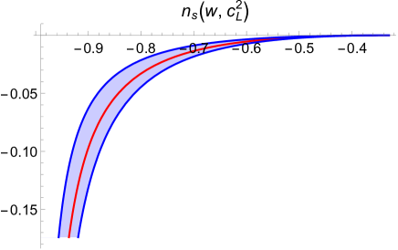
Figure 1: Tilt parameter $n_{s}$ contour lines as a function of $w$ and $c_{L}^{2}$ parameters, using the experimental constraint $n_{s}=0.96\pm 0.014$ with CL $95\%$ in the case of no tensor perturbations and no momentum-dependence of the tilt.

Such result is in agreement with [34]. Thus, $w$-Media inflation for a zero temperature solid is ruled out being the spectrum inevitably blue tilted when $c_{L}^{2}>0$.

Consider now the effect of $\delta\sigma$. In the case of a $w$-Media, $c_{b}^{2}=w$ and the condition (4.28) is trivially satisfied; the time dependence of the source term in (4.15) is

$$\gamma=-\frac{6\,w}{(1+3\,w)}\,,\qquad\Sigma_{k}=(-1)^{\gamma}\,\frac{\varphi^{\prime}_{in}}{\sqrt{1+w}}\,\left[\frac{(1+3\,w)\,(c_{L}^{2}-w)}{4\,c_{L}}\right]\,\delta\hat{\sigma}\,.$$ (5.19)

The size of $\Sigma_{k}$ is basically set by $\delta\sigma$ unless $w\approx-1$. From $(\ref{spectrum-deltasigma})$ we get

$${\cal P}^{(\delta\sigma)}\propto\frac{|\Sigma_{k}|^{2}\;k^{3}}{\epsilon}\,H_{in}^{-\frac{4}{1+3\,w}}\,;$$ (5.20)

moreover

$$\frac{{\cal P}^{(\delta\sigma)}}{{\cal P}_{\zeta^{(0)}}}\sim\frac{|\delta\sigma|^{2}}{\epsilon_{i}}\,k^{2\,\nu}\,(-t)^{-1+2\,\nu+\frac{4}{(1+3\,w)}}\,.$$ (5.21)

Such a ratio is time dependent if we take an almost flat tilt for ${\cal P}_{\zeta^{(0)}}$ with $\nu\approx\frac{3}{2}$

$$\frac{{\cal P}^{(\delta\sigma)}}{{\cal P}_{\zeta^{(0)}}}\sim\frac{|\delta\sigma|^{2}}{\epsilon_{i}}\,k^{2\,\nu}\,(-t)^{6\frac{(1+w)}{1+3\,w}}\,.$$ (5.22)

The conclusion is that the entropic contribution is in general dominant; thus a blue-tilted spectrum can turned in a red-tilted one by taking $\delta\sigma$ such that ${\cal P}^{(\delta\sigma)}$ is the dominant part of the spectrum with a red tilt. We will study such possibility in a separate paper [22] where the dynamics of $\delta\sigma$ will be analyzed in detail.

6 Gravitational Waves

Spin two perturbations are defined by

$$g_{00}=-a^{2}\,,\qquad g_{0i}=0\,,\qquad g_{ij}=a^{2}\left(\delta_{ij}+\chi_{ij}\right)\,.$$ (6.1)

For all media considered the dynamics of spin two modes during inflation can be derived from the following Lagrangian (Fourier basis)

$$L_{T}=\frac{a^{2}\,M_{\text{Pl}}^{2}}{2}\left[\chi_{ij}^{\prime}\chi_{ij}^{\prime}-\left(k^{2}+\frac{M_{2}}{a^{2}}\right)\chi_{ij}\chi_{ij}\right]\,.$$ (6.2)

The mass parameter $M_{2}$ in $c_{T}^{2}$, which in the scalar sector controls the amount of the anisotropic stress, it is also behind the dispersion relation for the propagation of the gravitational waves. By using (4.6), the equation of motion can be written as

$$\chi_{ij}^{\prime\prime}+\frac{2\,\beta}{t}\chi_{ij}^{\prime}+\chi_{ij}\left[k^{2}+\frac{6\,c_{T}^{2}\,\beta^{2}\,(1+w)}{t^{2}}\right]=0\,.$$ (6.3)

As usual, the quantum field $\chi_{ij}$ is made up of two polarizations

$$\chi_{ij}=\sum_{s=1}^{2}\varepsilon_{ij}^{s}\,\chi_{s}\,,\qquad\chi_{s}=\chi\,\hat{a}^{s}_{k}+\chi^{*}\,\hat{a}^{s\,\dagger}_{k}\,,$$ (6.4)

with modes

$$\begin{split}&\chi={\cal C}_{1}\,t^{\frac{1}{2}(1-2\beta)}H_{\nu_{T}}^{(1)}(-k\,t)+{\cal C}_{2}\,t^{\frac{1}{2}(1-2\,\beta)}H_{\nu_{T}}^{(2)}(-k\,t),\\ &\nu_{T}=\frac{1}{2}\sqrt{1-4\,\beta(1-\beta)-24\,c_{T}^{2}\,\beta^{2}\,(1+w)}\,.\end{split}$$ (6.5)

Taking into account a factor two due to polarization average, we get for the primordial tensor power spectrum

$${\cal P}_{T}=\frac{k^{3}}{\pi^{2}}|\chi|^{2}=\frac{4^{\nu_{T}-1}\,\Gamma(\nu_{T})^{2}\,H_{in}^{-2\,\beta}}{\pi^{3}\,M_{pl}^{2}}(-t)^{1-2\,\beta-2\,\nu_{T}}\,k^{3-2\,\nu_{T}}\,.$$ (6.6)

Once the tensor power spectrum is given, by using our previous results, we can compute the tensor to scalar ratio in the case of ${\cal R}$ and $\zeta$ separately. The entropic contribution is not in general suppressed by $\epsilon$ as for single field slow-roll inflation, but determined by $\delta\sigma$. The ratio is defined as

$$r_{A}=\frac{{\cal P}_{T}}{{\cal P}_{A}}=\frac{{\cal P}_{T}}{{\cal P}_{A}^{(0)}+{\cal P}_{A}^{(\delta\sigma)}}\,.$$ (6.7)

The suffix $A$ stands for $A=\zeta,\;{\cal R}$; indeed, being the Weinberg theorem typically violated the two power spectra must be studied separately. Taking $\delta\sigma$ of order $O(\sqrt{\epsilon_{i}})$, the two contributions of the total power spectrum are in general comparable with some notable exception. Hereafter, we will use the following definitions/relations

$$\frac{1}{r_{A}}=\frac{1}{r_{A}^{(0)}}+\frac{1}{r^{(\delta\sigma)}}\,,\qquad r_{A}^{(0)}=\frac{{\cal P}_{T}}{{\cal P}_{A}^{(0)}}\,,\qquad r^{(\delta\sigma)}=\frac{{\cal P}_{T}}{{\cal P}^{(\delta\sigma)}}\,.$$ (6.8)

Obviously there are two extreme regimes

1. $r_{A}^{(0)}\ll r^{(\delta\sigma)}\,\Rightarrow\,\frac{{\cal P}^{(\delta\sigma)}}{{\cal P}_{A}^{(0)}}\ll 1$ and $r_{A}\approx r_{A}^{(0)}$ ,

2. $r_{A}^{(0)}\gg r^{(\delta\sigma)}\,\Rightarrow\,\frac{{\cal P}^{(\delta\sigma)}}{{\cal P}_{A}^{(0)}}\gg 1$ and $r_{A}\approx r^{(\delta\sigma)}$ .

When the isentropic part is sub-dominant, the ratio is more or less unchanged with respect to the single field slow-roll scenario. If the entropic part is the dominant one, the ratio will be even more suppressed. Thus, the more interesting case is when the two contributions are comparable and this happens respectively when

• SSR: $c_{b}^{2}=\frac{2}{3}$;

• SR: $c_{b}^{2}=-1$;

• WM: If we consider $\nu\approx\frac{3}{2}$, the entropic part always dominates unless $w$ is not close to minus one.

Details are given in appendix D.

7 Post-Inflation Evolution: Instantaneous Reheating

The violation of the Weinberg theorem makes the inflationary regime less robust; after inflation ends, ${\cal R}$ and $\zeta$ will be not conserved for superhorizon modes, thus the reheating phase becomes crucial to make quantitative predictions on how the initial conditions for the hot universe era are set. More than analyzing specific reheating models we will try to focus as much as possible on general features, approximating reheating as instantaneous and taking place on a suitable time-like hypersurface where the Israel junction conditions [35] will be imposed. The transition hypersurface ${\cal T}$ is given in terms of a 4-dimensional scalar $q$ as $q=$constant, or expanding at the linear order in perturbation theory

$$\bar{q}+\delta q=\text{constant}\,.$$ (7.1)

We will denote by the subscript $f_{-}$ the quantity $f$ evaluated at the end of inflation, while with $f_{+}$ the same quantity evaluated at the end of reheating when the medium that had driven inflation has decayed into the standard components of the hot Universe. The change of $f$ across ${\cal T}$ will be written as $[f]_{\cal T}=f_{+}-f_{-}$. On ${\cal T}$, the equation of state suddenly changes from the value at end of inflation $w_{-}=-1+2\,\epsilon_{f}/3$ to $w_{+}=1/3$ in the radiation dominated phase. The junction conditions [36] can be written as

1. First Junction condition:
   $[h_{ab}]_{\cal T}=0$
   The induced metric $h_{ab}$ on ${\cal T}$ is continuous. In particular, at the background level this is equivalent to the continuity of the scale factor $a$. At the linear level the jump of $\phi$ is determined by $\delta q$ according with

   $$\left[-\phi+{\cal H}\frac{\delta q}{\bar{q}^{\prime}}\right]_{\cal T}=\left[\zeta_{q}\right]_{\cal T}=0\,.$$ (7.2)

   Namely,

   $$\zeta_{q}=-\phi+{\cal H}\frac{\delta q}{\bar{q}^{\prime}}$$ (7.3)

   represents the gauge invariant curvature perturbation of a constant $q$ hypersurfaces and it is continuous across ${\cal T}$.

2. Second Junction condition
   $\left[K_{ab}\right]_{\cal T}=0$
   We have assumed that no surface layer EMT tensor is present. In the absence of a localized EMT on ${\cal T}$, the extrinsic curvature $K_{ab}$ has to be continuous. At the background level, it implies the continuity of ${\cal H}$ across ${\cal T}$, namely $[{\cal H}]=0$. At the linear level from its diagonal part

   $$\left[\left(1-\frac{{\cal H}^{\prime}}{{\cal H}^{2}}\right)\left({\cal R}-\zeta_{q}\right)\right]_{\cal T}=0\,,$$ (7.4)

   while from the off-diagonal part

   $$\left[\frac{\delta q}{\bar{q}^{\prime}}\right]_{\cal T}=0\,.$$ (7.5)

   Together with the continuity of $\zeta_{q}$ leads to the continuity of $\phi$. Thus, the perturbation $\delta q$ can be characterized by a sharp jump during the transition.

The choice of no surface layer EMT is consistent with the form of our EMT: though $M_{2}$ and $\delta\sigma$ can have a finite jump, no $\delta$-like contribution is present. From the continuity of $\zeta_{q}$, the junction condition (7.4) tells that ${\cal R}$ must jump across ${\cal T}$ 

$$\epsilon_{+}\,\left({\cal R}_{+}-\zeta_{q}\right)=\epsilon_{f}\left({\cal R}_{-}-\zeta_{q}\right)\qquad\Rightarrow\qquad{\cal R}_{+}=\zeta_{q}+\frac{\epsilon_{f}}{\epsilon_{+}}\left({\cal R}_{-}-\zeta_{q}\right)\,,$$ (7.6)

A crucial point is that when the Weinberg theorem holds, whatever the hypersurface, $\zeta_{q}$ is conserved at superhorizon scales and $\zeta_{q}\approx\zeta_{q^{\prime}}|_{q\neq q^{\prime}}$; therefore the choice of the curvature perturbation does not matter. However, if the Weinberg theorem is violated, the quantity continuous across ${\cal T}$ will depend on the choice of $q$. In other words, the violation of the Weinberg theorem inevitably introduces a certain degree of dependence on the details of reheating.

If, as it usually done, one assumes that the instantaneous reheating takes place at $\rho=$const. [11] an issue emerges. From one hand, a medium-driven inflation will produce ${\cal R}\neq\zeta$ and at $\rho=$const. will transmit such a difference. On the other hand, a $\Lambda$CDM universe is incompatible with ${\cal R}\neq\zeta$. Indeed, the Weinberg theorem holds and the only source of non-conservation for ${\cal R}$ and $\zeta$ comes from entropic perturbations encoded in $\Gamma_{\Lambda\text{CDM}}$ defined by the following superhorizon dynamics

$${\cal R}^{\prime}=\zeta^{\prime}=\frac{{\cal H}\,\Gamma_{\Lambda\text{CDM}}}{\rho+p}\,,\qquad\text{with }{\cal R}=\zeta\,.$$ (7.7)

In general $\Gamma_{\Lambda\text{CDM}}$ is different from zero when the various species have different density perturbations in the presence of isocurvature modes; see for instance [9]. Let us discuss the isentropic ($\delta\sigma=0$) and the general adiabatic case separately.

7.1 Isentropic Inflation

Let us first assume $\delta\sigma=0$ and $\rho$=const. reheating. For the inflationary regimes of interest we have the following situation.

1. Super slow-roll
   The value of $\epsilon_{f}$ is so small that ${\cal R}_{+}=\zeta$; the comoving curvature sharply jumps assuming as final value the one of $\zeta$ at end of inflation. Differently from [10], the distinction between $\zeta$ and ${\cal R}$ is crucial. This is the only regime where reheating taking place at constant energy surface does not transmit the difference between ${\cal R}$ and $\zeta$ to the radiation dominated epoch.

2. Slow-roll
   At the end of inflation ${\cal R}$ and $\zeta$ are different if $c_{L}^{2}\neq 1$, see eq. (5.10), and

   $${\cal R}_{+}=\zeta+\frac{\epsilon_{f}}{\epsilon_{+}}\left({\cal R}_{-}-\zeta\right)=\zeta\left[1-\frac{\epsilon_{f}}{2}(c_{L}^{2}+1)\right]\,.$$ (7.8)

   As a result, a small difference between ${\cal R}$ and $\zeta$ is transmitted to the radiation phase suppressed by $\epsilon_{f}$. This difference cannot be explained using relative entropy perturbations after reheating in the standard $\Lambda$CDM. Such a difference can be attributed only to a particular dark sector [9, 30] where the Weinberg theorem is violated with or without intrinsic entropy perturbations.

3. $w$-Media
   $\epsilon_{f}$ is not in general small and the violation of the Weinberg theorem is still sizable and the same considerations for slow-roll applies.

7.2 Adiabatic Case

Let us now discuss the general case whit $\delta\sigma\neq 0$. The choice of a constant energy density hypersurface is dynamically justified only when entropy perturbations are absent during the two cosmological epochs. However, when the Weinberg theorem is violated this is not the only choice. The idea is to identify the scalar $q$ that can be considered constant during the transition. Suppose that the current $J^{\mu}=n\,u^{\mu}$ is conserved during reheating, intuitively we can imagine that the total relative number density $\frac{\delta n}{n}$ is continuous during the instantaneous transition, namely

$$\left[\frac{\delta n}{\bar{n}}\right]=0\,.$$ (7.9)

A dynamical derivation of the continuity of $\delta n/\bar{n}$ is given in appendix E. Taking as $n=$constant the reheating hypersurface, the junction conditions imply that the scalar curvature

$$\zeta_{n}=-\phi+{\cal H}\frac{\delta n}{\bar{n}^{\prime}}\,,$$ (7.10)

is continuous during the transition. After some manipulations, one can show that $\zeta_{n}$ is related to longitudinal phonons during inflation, namely

$$\zeta_{n}-=\frac{k^{2}}{3}\pi_{L}=\zeta-\frac{\bar{\varphi}^{\prime}\,\delta\sigma}{3\,a^{4}\,\rho\,(1+w)}\,.$$ (7.11)

The very same quantity, at the end of the reheating, when the universe is radiation dominated, is given by

$$\zeta_{n}=\zeta-\frac{\Gamma_{\Lambda\text{CDM}}}{3\,\rho\,(1+w)\,c_{s}^{2}}\,;$$ (7.12)

where $\Gamma_{\Lambda\text{CDM}}$ is the total entropic contribution coming from the possible difference in the density perturbations of the various components of the universe when isocurvature modes are present . Once again, if the transition takes place between two adiabatic phases for which $\Gamma=0$, $\zeta_{n}=\zeta$ is continuous and the difference between ${\cal R}$ and $\zeta$ is transmitted to the radiation dominated phase.
In the transition at $n=$const. the “standard” $\zeta$ is not continuous and its jump is fixed by the condition $[\zeta_{n}]=0$, while from (7.4) we can find the final value ${\cal R}_{+}$ of the comoving curvature perturbation at end of reheating. Thus

$$\begin{split}&[\zeta]=\left[\frac{\Gamma_{\text{eff}}}{3\,\rho\,(1+w)\,c_{s}^{2}}\right]\,,\\ &{\cal R}_{+}=\zeta_{n}+\frac{\epsilon_{f}}{\epsilon_{+}}\left({\cal R}_{-}-\zeta_{n}\right)\,.\end{split}$$ (7.13)

The effective quantity $\Gamma_{\text{eff}}$ is defined as follows:

$$\text{Inflation: }\Gamma_{\text{eff}}=-\frac{\bar{\varphi}^{\prime}}{a^{4}}\,c_{s}^{2}\,\delta\sigma\,,\qquad\text{Radiation: }\Gamma_{\text{eff}}=\Gamma_{\Lambda\text{CDM}}\,.$$ (7.14)

Imagine that during inflation the intrinsic entropy perturbation per particle $\delta\sigma$ is exactly zero. In this case

$$\zeta_{n}=\zeta_{n\,-}=\zeta^{(0)}_{-}\,,\qquad\Gamma_{\text{eff}}{}_{+}=\Gamma_{\Lambda\text{CDM}}\,.$$ (7.15)

As a consequence (LABEL:jumps) reduces to

$$\begin{split}&\zeta_{+}=\zeta^{(0)}_{-}+\frac{\Gamma_{\Lambda\text{CDM}}}{3\,\rho\,(1+w)\,c_{s}^{2}}|_{+}\\ &{\cal R}_{+}=\zeta^{(0)}_{-}+\frac{\epsilon_{f}}{\epsilon_{+}}\left({\cal R}^{(0)}-\zeta^{(0)}\right)|_{-}\,.\end{split}$$ (7.16)

Now we take into account that, in the radiation phase for $\Lambda$CDM, we can show that[9] at superhorizon scales:

$${\cal R}_{+}-\zeta_{+}=-\frac{\Gamma_{\Lambda\text{CDM}}}{3\,\rho\,(1+w)\,c_{s}^{2}}|_{+}+\frac{{\cal R}^{\prime}}{3\,{\cal H}\,c_{s}^{2}}|_{+}=0\,.$$ (7.17)

Consequently, we get the following crucial result

$${\cal R}_{+}=\zeta_{+}=\zeta^{(0)}_{-}+\frac{\epsilon_{f}}{\epsilon_{+}}\left({\cal R}^{(0)}-\zeta^{(0)}\right)|_{-}\,,$$ (7.18)

with the value of $\Gamma_{\Lambda\text{CDM}}$ fixed by inflation dynamics according with

$$\frac{\epsilon_{f}}{\epsilon_{+}}\left(\zeta^{(0)}-{\cal R}^{(0)}\right)|_{-}+\frac{\Gamma_{\Lambda\text{CDM}}}{3\,\rho\,(1+w)\,c_{s}^{2}}|_{+}=0\,.$$ (7.19)

The superhorizon value of ${\cal R}$ and $\Gamma_{\Lambda\text{CDM}}$ given by given by (7.18) and (7.19) can be used to set the initial conditions for the standard evolution of the universe. As anticipated, the bottom line is that the violation of the Weinberg theorem inflation triggers the generation of relative entropy perturbations, namely isocurvature modes, in $\Lambda$CDM.

Finally, let us consider the effect of an intrinsic entropy perturbations during inflation. In this case we have that

$$-\frac{\Gamma_{\text{eff}}}{3\,\rho\,(1+w)\,c_{s}^{2}}|_{-}=\alpha\,\zeta^{(\delta\sigma)}|_{-}\,,\qquad\zeta_{n}=\zeta_{-}^{(0)}+(1+\alpha)\zeta_{-}^{(\delta\sigma)}\,.$$ (7.20)

The value of the constant $\alpha$ is generically of order one, and its precise value depends on $c_{b}^{2}$. In this case, (LABEL:jumps) gives

$$\begin{split}&\zeta_{+}=\zeta^{(0)}_{-}+(1+\alpha)\,\zeta^{(\delta\sigma)}_{-}+\frac{\Gamma_{\Lambda\text{CDM}}}{3\,\rho\,(1+w)\,c_{s}^{2}}|_{+}\;\\ &{\cal R}_{+}=\zeta^{(0)}_{-}+(1+\alpha)\,\zeta^{(\delta\sigma)}_{-}+\frac{\epsilon_{f}}{\epsilon_{+}}\left({\cal R}^{(0)}-\zeta^{(0)}-\alpha\,\zeta^{(\delta\sigma)}\right)|_{-}\,.\end{split}$$ (7.21)

If we consider $\Lambda$CDM, we get a result similar to (7.18), with an additional contribution due to the presence of $\delta\sigma$

$$\begin{split}&\zeta_{+}={\cal R}_{+}=\zeta^{(0)}_{-}+(1+\alpha)\,\zeta^{(\delta\sigma)}_{-}+\frac{\epsilon_{f}}{\epsilon_{+}}\left({\cal R}^{(0)}-\zeta^{(0)}-\alpha\,\zeta^{(\delta\sigma)}\right)|_{-}\,;\\ &\frac{\epsilon_{f}}{\epsilon_{+}}\left(\zeta^{(0)}+\alpha\,\zeta^{(\delta\sigma)}-{\cal R}^{(0)}\right)|_{-}+\frac{\Gamma_{\Lambda\text{CDM}}}{3\,\rho\,(1+w)\,c_{s}^{2}}|_{+}=0\,;\end{split}$$ (7.22)

where we have used that ${\cal R}^{(\delta\sigma)}=\zeta^{(\delta\sigma)}$. Note that also the intrinsic $\zeta^{(\delta\sigma)}_{-}$ part is always suppressed by $\epsilon_{f}$. If we consider that after reheating with a very good precision accuracy: $\epsilon_{+}\approx 2\,,\;w_{+}\approx 1/3\,,\;c_{s}^{2}{}_{+}\approx 1/3$, we get that the $\Gamma_{\Lambda\text{CDM}}$ is

$$\Gamma_{\Lambda\text{CDM}}=\rho\left(1+w\right)|_{-}\,\left({\cal R}-\zeta-\alpha\,\zeta^{(\delta\sigma)}\right)|_{-}\,.$$ (7.23)

In conclusion, in the case of inflation driven by an isentropic medium, the choice of surface where the instantaneous reheating takes place is crucial to determine how the difference $({\cal R}-\zeta)$ is transmitted to the radiation phase. For both the choices of constant $\rho$ or $n$ hypersurface for reheating, the corresponding curvature perturbation $\zeta$ or $\zeta_{n}$ is continuous or characterized by a small jump proportional to $\epsilon_{f}$. On the contrary, the comoving curvature perturbation ${\cal R}$ sharply jumps in trying to match the value of $\zeta$ or $\zeta_{n}$ respectively. These above mentioned feature has a dramatic consequence on what scalar one uses to define scale invariant power spectrum: the only reasonable choice is $\zeta$ from which the tilt and tensor to scalar ratio are extracted.

8 Conclusions

In this paper, by using an effective field theory approach, we have studied in a systematic way inflation driven by a generic adiabatic medium, extending the previous works on fluid and solid inflation. The focus is on the violation of the Weinberg theorem during inflation which has two main sources: anisotropic stress (for solids) and entropic perturbations. A third mechanism, related to the peculiar background dynamics of the super slow-roll regime, plays a major role for fluids for which the standard slow-roll regime is not viable. In general, even if a media is adiabatic, a constant in time entropy per particle $\sigma(\vec{x})$ can be present. As a result, when the medium is non-barotropic, the entropy per particle perturbation $\delta\sigma$ acts as a source term in the dynamical equation for both the comoving curvature perturbation ${\cal R}$ and the uniform curvature perturbation $\zeta$. At superhorizon scales, both ${\cal R}$ and $\zeta$ are not constant in time with $\zeta\neq{\cal R}$. At the level of power spectrum, we get that the scalar amplitude of momentum $k$ keeps growing until inflation ends, even if $k$ is superhorizon, moreover an additional contribution due to $\delta\sigma$ is present. Being $\delta\sigma$ strictly constant for an adiabatic medium, its contribution to the power spectrum is an undetermined function of the comoving momentum. It is interesting to note that, when the adiabaticity condition is removed, $\delta\sigma$ will be dynamically determined with $\delta\sigma^{\prime}=0$ at superhorizon scales; thus, an adiabatic medium can be considered as a convenient simplified model to describe a generic non-dissipative medium at superhorizon scales. The violation of the Weinberg theorem is also relevant for the reheating phase. Considering an instantaneous reheating, taking place on a suitable spacelike hypersurface, the variation of $\zeta$ and ${\cal R}$ is essentially geometric and encoded in the Israel junction conditions.

In the case $\delta\sigma=0$ ( both during inflation and radiation domination ) energy conservation suggests that the instantaneous reheating takes place on $\rho=$ constant hypersurface with $\zeta$ continuous while ${\cal R}$ jumps. In fluid inflation, the power spectrum of $\zeta$ is almost scale free but it requires $c_{s}^{2}\gg 1$, which makes fluid inflation not very exciting. In the slow-roll case, a small violation of the Weinberg theorem during the radiation phase is present, resulting in a difference $({\cal R}-\zeta)|_{+}$ which is order $\epsilon$. Similar considerations apply to the case of $w$-media inflation, with the only difference that $\epsilon$ is not small in general, however it predicts a blue-tilted power spectrum which is ruled out by observations.

The violation of the Weinberg theorem is also important during reheating. We have shown that, in the instantaneous approximation, reheating on $\rho=$constant hypersurface makes strictly speaking impossible to connect inflation with a standard radiation dominated $\Lambda$CDM universe. Indeed, to take into account the difference of $\zeta$ and ${\cal R}$ a non-standard dark energy sector is needed. Insisting on $\Lambda$CDM requires to reconsider the reheating hypersurface. Our analysis shows that in the contest of adiabatic media is rather natural to take the constant particle number hypersurface across which the corresponding curvature perturbation $\zeta_{n}$ is continuous . Applying the junction conditions we arrive at the conclusion that the difference $({\cal R}-\zeta)|_{-}$ during inflation and any intrinsic entropic contribution $\zeta^{(\delta\sigma)}$ induces a contribution of isocurvature perturbations on the top of the adiabatic ones for $\Lambda$CDM radiation dominated epoch. Furthermore, in slow roll, the change of $\zeta$ is small and order $\epsilon$. Consequently, we can still use the $\zeta$ power spectrum to define the tilt parameter and the tensor to scalar ratio. It is also interesting to point out that the additive entropic contribution to the power spectrum can be used as seed to form primordial black holes that could constitute an important part of dark matter in the universe. Finally, let us briefly comment on primordial non-Gaussianity. The local $f_{NL}$ parameter in the squeezed configuration which is most constrained by observations [37], plays a crucial role in the CMB angular bispectrum [38, 39, 40], and in the scale dependence of the halo bias [41, 42, 43]. Here, the validity of the Weinberg Theorem is strictly related with the validity of the Maldacena consistency relations for the squeezed configuration in single field inflation [44]. Thus the violation of the Weinberg theorem directly implies the possibility to get features which are considerably different from the single field inflation predictions. While primordial non-Gaussianity for an isentropic solid was already computed in [11], the case for a general media which has two scalar modes is presently unknown and we hope to report on it soon.

Appendix A Masses

The explicit values of the mass parameters in terms of $U$ and its derivatives, are given in the case of a FLRW spacetime in conformal time by

$$\begin{split}&M_{0}=\frac{\phi^{\prime 2}}{2\,M_{\text{Pl}}^{2}}\left[a^{2}\left(U_{Y^{2}}-2\;U_{X}\right)-4\;a\;\phi^{\prime}\;U_{XY}+4\;U_{X^{2}}\,\phi^{\prime 2}\right],\\ &M_{1}=\frac{2\,\phi^{\prime 2}}{M_{\text{Pl}}^{2}}\left(\sum_{n=0}^{3}\;a^{-2\;n}\;U_{y_{n}}+a^{2}\;U_{X}\right),\\ &M_{2}=-\frac{2}{M_{\text{Pl}}^{2}}\;\sum_{n=1}^{3}\;n^{2}\,a^{2(2-n)}\;U_{\tau_{n}},\\ &M_{3}=\frac{1}{M_{\text{Pl}}^{2}}\left(2\sum_{m,n=1}^{3}m\,n\,a^{-2m-2n+4}\,U_{\tau_{m}\tau_{n}}+2\sum_{n=1}^{3}n\,a^{1-2n}\;\,U_{b\tau_{n}}-\sum_{n=1}^{3}a^{4-2n}\,U_{\tau_{n}}+\frac{1}{2\,a^{2}}U_{b^{2}}\right)\,,\\ &M_{4}=\frac{\phi^{\prime}}{2\,M_{\text{Pl}}^{2}}\left(2\,\sum_{n=1}^{3}a^{3-2n}\,U_{Y\tau_{n}}-a^{3}\,U_{Y}+U_{bY}\right)\\ &\,\;\qquad+\frac{\phi^{\prime 2}}{M_{\text{Pl}}^{2}}\left(-2\,\sum_{n=1}^{3}\,a^{2-2n}\;U_{X\tau_{n}}+a^{2}\,U_{X}-\frac{1}{a}\,U_{bX}\right);\end{split}$$ (A.1)

Appendix B $\zeta$ Evolution

Proceeding as for ${\cal R}$ one can write down an evolution equation for $\zeta$ only which has the form

$$\left[\zeta^{\prime}\,\frac{6a^{2}(w+1)\mathcal{H}^{2}}{2k^{2}+9(w+1)\mathcal{H}^{2}}\right]^{\prime}+m_{\zeta}^{2}\,\zeta+B_{\sigma}\,\delta\hat{\sigma}=0\,,$$ (B.1)

with

$$\begin{split}&m_{\zeta}^{2}=6\,a^{2}\,\mathcal{H}^{2}\,(1+w)\frac{\left[2\,k^{4}\,c_{L}^{2}+9\,k^{2}\,\mathcal{H}^{2}\,(w+1)\left(8\,c_{T}^{2}-1\right)+54\,\mathcal{H}^{4}\,(w+1)^{2}\,c_{T}^{2}\right]}{\left[2\,k^{2}+9\,(w+1)\,\mathcal{H}^{2}\right]^{2}}\,;\\ &B_{\sigma}=\bar{\varphi}^{\prime}\frac{4\,k^{4}(c_{L}^{2}-c_{b}^{2})+4\,k^{2}\,\,F_{2}+9\,(1+w)\,F_{0}}{\left[6\left(2k^{2}+9(w+1)\mathcal{H}^{2}\right)^{2}\right]}\\ &F_{2}=\mathcal{H}^{2}\left[3\,c_{b}^{2}\left(3\,c_{b}^{2}-3\,c_{L}^{2}+4\,c_{T}^{2}-2\right)+6\,c_{L}^{2}+12\,w\,c_{T}^{2}+4\,c_{T}^{2}\right]+\mathcal{H}\left(3\,c_{L}^{2}{}^{\prime}-4\,c_{T}^{2}{}^{\prime}-3\,c_{b}^{2}{}^{\prime}\right)\,;\\ &F_{0}={\cal H}^{4}\Big{\{}c_{b}^{2}\left(48\,c_{T}^{2}-36\,c_{L}^{2}+9\,w-9\right)+18\,c_{b}^{4}+3\,w\left(8\,c_{T}^{2}-3\,c_{L}^{2}\right)+2\left(3\,c_{L}^{2}-4\,c_{T}^{2}\right){}^{2}+9\,c_{L}^{2}\Big{\}}\\ &\quad+{\cal H}^{3}\left[6(c_{L}^{2}{}^{\prime}-\,c_{b}^{2}{}^{\prime})-8\,c_{T}^{2}{}^{\prime}\right]\,.\end{split}$$ (B.2)

Appendix C Dynamics of entropy perturbations on superhorizon scales

According to [17], when $M_{1}\neq 0$, at superhorizon scales the entropy per particle perturbation $\delta\sigma$ evolution is described by

$$\left[\delta\sigma^{\prime}\frac{\bar{\varphi}^{\prime}{}^{2}\left(6\,a^{2}\,(1+w\,){\cal H}^{2}+M_{1}\right)}{6\,a^{2}\,M_{1}(1+w)\,{\cal H}^{2}}\right]^{\prime}=0\,,\qquad\frac{k^{2}}{{\cal H}^{2}}\ll 1\,,$$ (C.1)

which can be easily integrated to give

$$\delta\sigma=\delta\sigma_{0}+\delta\sigma_{1}\,\int^{t}dt^{\prime}\,\frac{1}{M_{pl}\,\varphi^{\prime}{}^{2}}\,\frac{6\,a^{2}\,(1+w)\,{\cal H}^{2}\,M_{1}}{M_{1}+6\,a^{2}\,(1+w)\,{\cal H}^{2}}\,.$$ (C.2)

Let us parametrize the $M_{1}$ time dependence as follows

$$M_{1}=m_{1}\,a^{\lambda}_{1}\,.$$ (C.3)

If we assume the constant $m_{1}$ to be not too small, we get at the leading order in the slow-roll parameter $\epsilon_{i}$

$$\delta\sigma=\delta\sigma_{0}+\delta\sigma_{1}\frac{4\,\epsilon_{i}\,H_{in}^{-6\,c_{b}^{2}(1+\epsilon_{i})-\eta}}{\left[1+6\,c_{b}^{2}(1+\epsilon_{i})+\eta\right]\,M_{pl}\,\varphi_{in}^{\prime}{}^{2}}\,(-t)^{-1-6\,c_{b}^{2}(1+\epsilon_{i})-\eta}.$$ (C.4)

The above result holds in the SSR and SR regimes. Thus, the absence of entropy growing modes is ensured by the condition

$$c_{b}^{2}<-\frac{(1+\eta)}{6(1+\epsilon_{i})}\,\Rightarrow\;\text{SSR}\,:\;c_{b}^{2}<-\frac{1}{6}(1+\eta),\;\;\text{SR}\,:\;c_{b}^{2}<-\frac{1}{6}\,.$$ (C.5)

Note that this relation is compatible with (4.28).

Appendix D Tensor to scalar ratio

Let us analyze the tensor to scalar ratio $r$ in the relevant inflationary regimes. For fluid inflation in the super slow-roll regime, when $\beta=-1$ and $w\approx-1$, we get $\nu_{T}=3/2$ and the tensor spectrum is exactly scale-free with $n_{T}=1$

$${\cal P}_{T}=\frac{1}{2}\frac{H_{in}^{2}}{\pi^{2}\,M_{pl}^{2}}\,.$$ (D.1)

For $r$, depending on the value of $c_{b}^{2}$, we have the following possible cases.

1. $\frac{2}{3}<c_{b}^{2}<3$
   For both $\zeta$ and ${\cal R}$, we have ${\cal P}^{(\delta\sigma)}\ll{\cal P}^{(0)}$ and thus the total scalar is dominated by the isentropic part $r^{(0)}$. In particular

   $$\begin{split}&r_{\zeta}^{(0)}=9\,2^{10+\eta}\frac{\Gamma\left(\frac{3}{2}\right)^{2}\,c_{s}^{-5-\eta}}{\Gamma\left(-\frac{(5+\eta)}{2}\right)^{2}}\left(-k\,t\right)^{-(10+\eta)}\,\epsilon(t)\,,\\ &r_{\cal R}^{(0)}=2^{7+\eta}\frac{\Gamma\left(\frac{3}{2}\right)^{2}\,c_{s}^{-5-\eta}}{\Gamma\left(-\frac{(3+\eta)}{2}\right)^{2}}\left(-k\,t\right)^{-(6+\eta)}\,\epsilon(t)\,.\end{split}$$ (D.2)

   The difference between ${\cal R}$ and $\zeta$ is important, indeed $r_{\cal R}^{(0)}/r_{\zeta}^{(0)}\sim(-k\,t)^{4}$; thus $r_{\cal R}^{(0)}$ is much smaller then $r_{\zeta}^{(0)}$ in the superhorizon limit. This was not noticed in [10].

2. $c_{b}^{2}=\frac{2}{3}$
   ${\cal P^{\delta\sigma}}\sim{\cal P}^{(0)}$. The entropic part is comparable with the standard one.

3. $c_{b}^{2}<\frac{2}{3}$
   In this case, ${\cal P}^{(\delta\sigma)}\gg{\cal P}^{(0)}$ and thus the total $r$ is close to $r^{(\delta\sigma)}$ with

   $$r^{(\delta\sigma)}\sim\,\frac{\epsilon_{i}^{2}}{|\delta\sigma|^{2}}\,k^{-3}\,t^{-6\,(1+c_{b}^{2})-2\,\eta}\,,$$ (D.3)

   setting $\eta=-10$ for a flat scalar spectrum, again for $|k\,t|\ll 1$ the ration goes to zero very fast.

Clearly, even in the presence of entropic perturbations, in fluid inflation the tensor to scalar ratio is vanishingly small.
Consider now slow-roll inflation for solids. In this case

$$\nu_{T}=\frac{3}{2}+\epsilon-\frac{4}{3}\,\epsilon\,c_{T}^{2}\,,\qquad{\cal P}_{T}=\frac{1}{2}\,\frac{H_{in}^{2}}{\pi^{2}\,M_{pl}^{2}}\;t^{\frac{8}{3}\,\epsilon\,c_{T}^{2}}\;k^{-2\,\epsilon+\frac{8}{3}\,\epsilon\,c_{T}^{2}}.$$ (D.4)

Again, $c_{b}^{2}$ is an important parameter for the tensor to scalar ratio.

1. $-1<c_{b}^{2}<-\frac{1}{3}$
   The isentropic part of the power spectrum is dominant and $r$ will be practically equal to $r^{(0)}$ with

   $$r^{(0)}_{\cal R}=4\,c_{L}\,\epsilon_{i}\,k^{\eta}\,,\qquad r^{(0)}_{\zeta}=r_{\cal R}\,c_{L}^{4}.$$ (D.5)

2. $c_{b}^{2}=-1$
   ${\cal P^{\delta\sigma}}\sim{\cal P}^{(0)}$. The entropic part is comparable with the standard one.

3. $c_{b}^{2}<-1$
   The entropic part of the power spectrum is dominant and of the order

   $$r^{(\delta\sigma)}\sim\frac{\epsilon_{i}^{2}}{|\delta\sigma|^{2}}\,k^{-3}\,(-t)^{-6\,(1+c_{b}^{2})}\,;$$ (D.6)

   it is completely analogous to fluid inflation and the tensor to scalar ratio is strongly suppressed.

Finally, let us consider $w$-media inflation, for which

$$\nu_{T}=-\frac{3}{2\,(1+3\,w)}\,\sqrt{(w-1)^{2}-8\,(1+w)\,(c_{L}^{2}-w)}=\nu\,.$$ (D.7)

Taking for instance $\nu_{T}\approx\frac{3}{2}$ which gives a blue tilt with $c_{L}^{2}>0$

$${\cal P_{T}}=\frac{H_{in}^{-2\,\beta}\,(-t)^{-\frac{1}{2}-2\,\beta}}{2\,\pi^{2}\,M_{pl}^{2}}\,.$$ (D.8)

Being $\nu_{T}=\nu$, the isentropic tensor to scalar ratio is time and scale independent

$$r^{(0)}_{\cal R}=\frac{6\,(w+1)}{c_{L}^{2\,(1+\nu)}}\,,\qquad r_{\zeta}=r^{(0)}_{\cal R}\,\frac{4\,c_{L}^{4}}{(1+3\,w)^{2}}\,.$$ (D.9)

As discussed in the previous sections, being in this case ${\cal P}^{(\delta\sigma)}\gg{\cal P}^{(0)}$, the entropic contribution will be the dominant one and the computation of $r^{(\delta\sigma)}$ will be necessary

$$r^{(\delta\sigma)}\sim\frac{1}{(1+3\,w)^{2}}\frac{\epsilon_{i}^{2}}{|\delta\sigma|^{2}}\,k^{-3}\,(-t)^{-6\,\frac{(1+w)}{1+3\,w}}\,.$$ (D.10)

Appendix E Reheating hypersurface

As discussed in section 7, the choice of a constant energy density as the reheating hypersurface is not the only option when the Weinberg theorem is violated. Following [45], we will study how reheating can take place on a different surface. Let us start, by using the $00$ component of the linearized Einstein equations, we get

$${\cal R}-\zeta=\frac{2}{9}\frac{k^{2}\,\phi}{(1+w)\,{\cal H}^{2}}\,,$$ (E.1)

We can generalize eq. (3.13) as follows

$${\cal R}^{\prime}=3\,{\cal H}\,c_{L}^{2}\,\left({\cal R}\,\,\frac{c_{s}^{2}}{c_{L}^{2}}-\zeta\right)+\frac{{\cal H}\,\tilde{\Gamma}}{\rho\,(1+w)}\,.$$ (E.2)

In the hydrodynamical approximation, the above relation holds before and after inflation. During inflation scalar anisotropic stress is encoded in $c_{L}^{2}$ through $c_{T}^{2}$ and

$$\tilde{\Gamma}=\frac{\varphi^{\prime}}{a^{4}}\,(c_{b}^{2}-c_{L}^{2})\,\delta\sigma\,.$$ (E.3)

During radiation domination, taking for simplicity $\Lambda$CDM constituted by a collection of isentropic fluids, anisotropic terms are absent and $c_{L}\to c_{s}$, while the $\tilde{\Gamma}$ reduces to

$$\tilde{\Gamma}=\Gamma_{\Lambda\text{CDM}}=\Gamma_{rel}\,.$$ (E.4)

Integrating (E.2) along the transition, we can estimate the jump of ${\cal R}$, extending the analysis of [45]; namely

$$\left[{\cal R}\right]=\int_{-}^{+}c_{s}^{2}\,\theta^{2}\,\left(\frac{2}{3}\,\frac{a^{2}}{{\cal H}}\,k^{2}\,\phi+\frac{{\cal H}\,\Gamma_{\text{eff}}}{\rho\,(1+w)\,c_{s}^{2}\,\theta^{2}}\right)\,dt\,,$$ (E.5)

where $\theta$ is given by

$$\theta=\frac{1}{a\,\sqrt{1+w}}\,.$$ (E.6)

$\Gamma_{\text{eff}}$ stands for the part of the $\Gamma$ which can give a contribution during the integration, i.e:

$$\text{Inflation: }\Gamma_{\text{eff}}=-\frac{\bar{\varphi}^{\prime}}{a^{4}}\,c_{s}^{2}\,\delta\sigma\,,\qquad\text{Radiation: }\Gamma_{\text{eff}}=\Gamma_{\Lambda\text{CDM}}\,.$$ (E.7)

Using the relation

$$c_{s}^{2}\,\theta^{2}=\frac{\rho}{3\,a^{2}\,{\cal H}}\left(\frac{1}{\rho+p}\right)^{\prime}-\frac{\rho}{a^{2}(\rho+p)}\,,$$ (E.8)

and integrating by parts we get

$$\left[{\cal R}\right]=\left[\frac{1}{3}\,\frac{k^{2}\,\phi}{{\cal H}^{2}\,\epsilon}+\frac{\Gamma_{\text{eff}}}{3\,\rho\,(1+w)\,c_{s}^{2}}\right]\,,$$ (E.9)

which, thanks to (E.1), is equivalent to

$$\left[\zeta-\frac{\Gamma_{\text{eff}}}{3\,\rho\,(1+w)\,c_{s}^{2}}\right]=[\zeta_{q}]=0\,.$$ (E.10)

Eq. (E.10) can also be interpreted the continuity of the curvature of a suitable $q=$const. hypersurface during the transition. By definition, we get

$$\frac{\delta q}{\bar{q}^{\prime}}=\frac{\delta\rho}{\bar{\rho}^{\prime}}-\frac{\Gamma_{\text{eff}}}{3\,\rho\,{\cal H}\,(1+w)\,c_{s}^{2}}\,.$$ (E.11)

As a matter of fact, $q$ is a linear combination of $\rho$ and total entropy per particle $\sigma$. In particular during inflation we can take $q=n$, where $n$ is the medium number density; thus

$$\zeta_{n}=\frac{k^{2}}{3}\pi_{L}=\zeta+\frac{\bar{\varphi}^{\prime}\,\delta\sigma}{12\,a^{2}\,\epsilon\,{\cal H}^{2}\,M_{pl}^{2}}=-\phi+{\cal H}\,\frac{\delta n}{\bar{n}^{\prime}}\,.$$ (E.12)

On the other hand, during radiation domination, one can show that taking $n=\sum_{i}\,n_{i}(\rho_{i},\sigma_{i})$, one gets

$$\zeta_{n}{}_{+}=\zeta_{+}-\frac{\Gamma_{\Lambda\text{CDM}}}{3\,\rho\,(1+w)\,c_{s}^{2}}\,;$$ (E.13)

the sum in the definition of $n$ refers to the different fluid components during $\Lambda$CDM. Thus, we have just demonstrated that $\zeta_{n}$ is continuous in the transition from inflation to radiation domination , coherently with the assumption in section 7

$$\left[\frac{\delta n}{n}\right]=-3\,\left[{\cal H}\,\frac{\delta n}{\bar{n}^{\prime}}\right]=0\,.$$ (E.14)

References

• [1] S. Weinberg. Adiabatic modes in cosmology. Phys. Rev., D67:123504, 2003.
• [2] S. Weinberg. Cosmology. Oxford Univ. Press, 2008.
• [3] Clifford Cheung, Paolo Creminelli, A. Liam Fitzpatrick, Jared Kaplan, and Leonardo Senatore. The Effective Field Theory of Inflation. JHEP, 03:014, 2008.
• [4] Steven Weinberg. Effective Field Theory for Inflation. Phys. Rev., D77:123541, 2008.
• [5] William H. Kinney. Horizon crossing and inflation with large eta. Phys. Rev., D72:023515, 2005.
• [6] Mohammad Hossein Namjoo, Hassan Firouzjahi, and Misao Sasaki. Violation of non-Gaussianity consistency relation in a single field inflationary model. EPL, 101(3):39001, 2013.
• [7] Hayato Motohashi, Alexei A. Starobinsky, and Jun’ichi Yokoyama. Inflation with a constant rate of roll. JCAP, 1509(09):018, 2015.
• [8] M. Akhshik, H. Firouzjahi, and S. Jazayeri. Effective Field Theory of non-Attractor Inflation. JCAP, 1507(07):048, 2015.
• [9] Marco Celoria, Denis Comelli, and Luigi Pilo. Intrinsic Entropy Perturbations from the Dark Sector. JCAP, 1803(03):027, 2018.
• [10] X. Chen, H. Firouzjahi, M. H. Namjoo, and M. Sasaki. Fluid Inflation. JCAP, 1309:012, 2013.
• [11] S. Endlich, A. Nicolis, and J. Wang. Solid Inflation. JCAP, 1310:011, 2013.
• [12] S. Matarrese. On the Classical and Quantum Irrotational Motions of a Relativistic Perfect Fluid. 1. Classical Theory. Proc. Roy. Soc. Lond., A401:53–66, 1985.
• [13] S. Dubovsky, T. Gregoire, A. Nicolis, and R. Rattazzi. Null energy condition and superluminal propagation. JHEP, 03:025, 2006.
• [14] S. Dubovsky, L. Hui, A. Nicolis, and D.T. Son. Effective field theory for hydrodynamics: thermodynamics, and the derivative expansion. Phys. Rev., D85:085029, 2012.
• [15] G. Ballesteros and B. Bellazzini. Effective perfect fluids in cosmology. JCAP, 1304:001, 2013.
• [16] G. Ballesteros, D. Comelli, and L. Pilo. Thermodynamics of perfect fluids from scalar field theory. Phys. Rev., D94(2):025034, 2016.
• [17] Marco Celoria, Denis Comelli, and Luigi Pilo. Fluids, Superfluids and Supersolids: Dynamics and Cosmology of Self Gravitating Media. JCAP, 1709(09):036, 2017.
• [18] Simeon Bird, Ilias Cholis, Julian B. Muñoz, Yacine Ali-Haïmoud, Marc Kamionkowski, Ely D. Kovetz, Alvise Raccanelli, and Adam G. Riess. Did LIGO detect dark matter? Phys. Rev. Lett., 116(20):201301, 2016.
• [19] Misao Sasaki, Teruaki Suyama, Takahiro Tanaka, and Shuichiro Yokoyama. Primordial Black Hole Scenario for the Gravitational-Wave Event GW150914. Phys. Rev. Lett., 117(6):061101, 2016. [erratum: Phys. Rev. Lett.121,no.5,059901(2018)].
• [20] Sebastien Clesse and Juan García-Bellido. Detecting the gravitational wave background from primordial black hole dark matter. Phys. Dark Univ., 18:105–114, 2017.
• [21] J. R. Espinosa, D. Racco, and A. Riotto. Cosmological Signature of the Standard Model Higgs Vacuum Instability: Primordial Black Holes as Dark Matter. Phys. Rev. Lett., 120(12):121301, 2018.
• [22] Marco Celoria, Denis Comelli, Luigi Pilo, and Rocco Rollo. In Preparation. 2019.
• [23] G. Ballesteros, D. Comelli, and L. Pilo. Massive and modified gravity as self-gravitating media. Phys. Rev., D94(12):124023, 2016.
• [24] Marco Celoria, Denis Comelli, and Luigi Pilo. Sixth mode in massive gravity. Phys. Rev., D98(6):064016, 2018.
• [25] Alan H. Guth. The Inflationary Universe: A Possible Solution to the Horizon and Flatness Problems. Phys. Rev., D23:347–356, 1981. [Adv. Ser. Astrophys. Cosmol.3,139(1987)].
• [26] Andrei D. Linde. A New Inflationary Universe Scenario: A Possible Solution of the Horizon, Flatness, Homogeneity, Isotropy and Primordial Monopole Problems. Phys. Lett., 108B:389–393, 1982. [Adv. Ser. Astrophys. Cosmol.3,149(1987)].
• [27] Andreas Albrecht and Paul J. Steinhardt. Cosmology for Grand Unified Theories with Radiatively Induced Symmetry Breaking. Phys. Rev. Lett., 48:1220–1223, 1982. [Adv. Ser. Astrophys. Cosmol.3,158(1987)].
• [28] David Langlois, Sebastien Renaux-Petel, Daniele A. Steer, and Takahiro Tanaka. Primordial perturbations and non-Gaussianities in DBI and general multi-field inflation. Phys. Rev., D78:063523, 2008.
• [29] Frederico Arroja, Shuntaro Mizuno, and Kazuya Koyama. Non-gaussianity from the bispectrum in general multiple field inflation. JCAP, 0808:015, 2008.
• [30] Marco Celoria, Denis Comelli, and Luigi Pilo. Self-gravitating $\Lambda$-media. JCAP, 1901(01):057, 2019.
• [31] Guillermo Ballesteros, Jose Beltran Jimenez, and Mauro Pieroni. Black hole formation from a general quadratic action for inflationary primordial fluctuations. JCAP, 1906(06):016, 2019.
• [32] E. Komatsu et al. Five-Year Wilkinson Microwave Anisotropy Probe (WMAP) Observations: Cosmological Interpretation. Astrophys. J. Suppl., 180:330–376, 2009.
• [33] Y. Akrami et al. Planck 2018 results. X. Constraints on inflation. Submitted to A&A, 2018.
• [34] Michael Sitwell and Kris Sigurdson. Quantization of Perturbations in an Inflating Elastic Solid. Phys. Rev., D89(12):123509, 2014.
• [35] W. Israel. Singular hypersurfaces and thin shells in general relativity. Nuovo Cim., B44S10:1, 1966. [Nuovo Cim.B44,1(1966)].
• [36] Nathalie Deruelle and Viatcheslav F. Mukhanov. On matching conditions for cosmological perturbations. Phys. Rev., D52:5549–5555, 1995.
• [37] Y. Akrami et al. Planck 2018 results. IX. Constraints on primordial non-Gaussianity. 2019.
• [38] N. Bartolo, S. Matarrese, and A. Riotto. Non-Gaussianity in the Cosmic Microwave Background Anisotropies at Recombination in the Squeezed limit. JCAP, 1202:017, 2012.
• [39] Enrico Pajer, Fabian Schmidt, and Matias Zaldarriaga. The Observed Squeezed Limit of Cosmological Three-Point Functions. Phys. Rev., D88(8):083502, 2013.
• [40] Giovanni Cabass, Enrico Pajer, and Fabian Schmidt. How Gaussian can our Universe be? JCAP, 1701(01):003, 2017.
• [41] Nicola Bartolo, Sabino Matarrese, and Antonio Riotto. Signatures of primordial non-gaussianity in the large-scale structure of the universe. Journal of Cosmology and Astroparticle Physics, 2005(10):010–010, oct 2005.
• [42] Neal Dalal, Olivier Doré, Dragan Huterer, and Alexander Shirokov. Imprints of primordial non-gaussianities on large-scale structure: Scale-dependent bias and abundance of virialized objects. Phys. Rev. D, 77:123514, Jun 2008.
• [43] Roland de Putter, Olivier Doré, and Daniel Green. Is There Scale-Dependent Bias in Single-Field Inflation? JCAP, 1510(10):024, 2015.
• [44] Juan Martin Maldacena. Non-Gaussian features of primordial fluctuations in single field inflationary models. JHEP, 05:013, 2003.
• [45] Viatcheslav Mukhanov. Physical Foundations of Cosmology. Cambridge Univ. Press, Cambridge, 2005.