A New Recurrent Plug-and-Play Prior Based on the Multiple Self-Similarity Network

Abstract

Recent work has shown the effectiveness of the plug-and-play priors (PnP) framework for regularized image reconstruction. However, the performance of PnP depends on the quality of the denoisers used as priors. In this letter, we design a novel PnP denoising prior, called multiple self-similarity net (MSSN), based on the recurrent neural network (RNN) with self-similarity matching using multi-head attention mechanism. Unlike traditional neural net denoisers, MSSN exploits different types of relationships among non-local and repeating features to remove the noise in the input image. We numerically evaluate the performance of MSSN as a module within PnP for solving magnetic resonance (MR) image reconstruction. Experimental results show the stable convergence and excellent performance of MSSN for reconstructing images from highly compressive Fourier measurements.

1 Introduction

Model-based image reconstruction is often formulated as the following optimization problem

$$\operatorname*{argmin}\limits_{\bm{x}}f(\bm{x})\;\;\;\;\;\text{with}\;\;\;\;\;f(\bm{x})=g(\bm{x})+h(\bm{x})$$ (1)

where $\bm{x}$ is the unknown image, $g$ is the data-fidelity term that penalizes the mismatch to the measurements, and $h$ is the regularizer that imposes a prior knowledge on the unknown. Over the years, many different regularizers have been proposed for the reconstruction task, including nonnegativity, transform-domain sparsity, and self-similarity [1, 2, 3, 4]. Additionally, a variety of proximal algorithms [5] have been developed to deal with the large amount of data and nondifferentiable regularizers. Two popular such algorithms are accelerated proximal gradient method (APGM) [6, 7, 8, 9] and alternating direction method of multipliers (ADMM) [10, 11, 12, 13].

Recently, Venkatakrishnan et al. [14] introduced a powerful plug-and-play priors (PnP) framework. They leveraged the mathematical equivalence of the proximal operator to denoising to infuse state-of-the-art image denoisers, such as BM3D [15], WNNM [16], TNRD [17], or DnCNN [18], into iterative algorithms. Although, PnP does not generally minimize any explicit objective function $f$, its effectiveness has been successfully validated on multiple imaging inverse problems [19, 20, 21, 22, 23, 24, 25, 26, 27, 28, 29, 30, 31].

Since the denoiser is the only source of prior knowledge in PnP, improving it can significantly boost the performance of the recovery. Recently, non-local neural network based denoisers were shown to achieve the state-of-the-art performance on several image denoising tasks [32, 33]. In this letter, we propose a new denoiser called multiple self-similarity net (MSSN), based on a recurrent neural network (RNN) and multi-head attention (MA) mechanism, to enhance the joint processing of non-local features. We validate our MSSN denoiser by infusing it into PnP-APGM for magnetic resonance (MR) image reconstruction. We show that PnP equipped with MSSN outperforms several state-of-the-art denoiser priors by enabling imaging from highly compressive measurements.

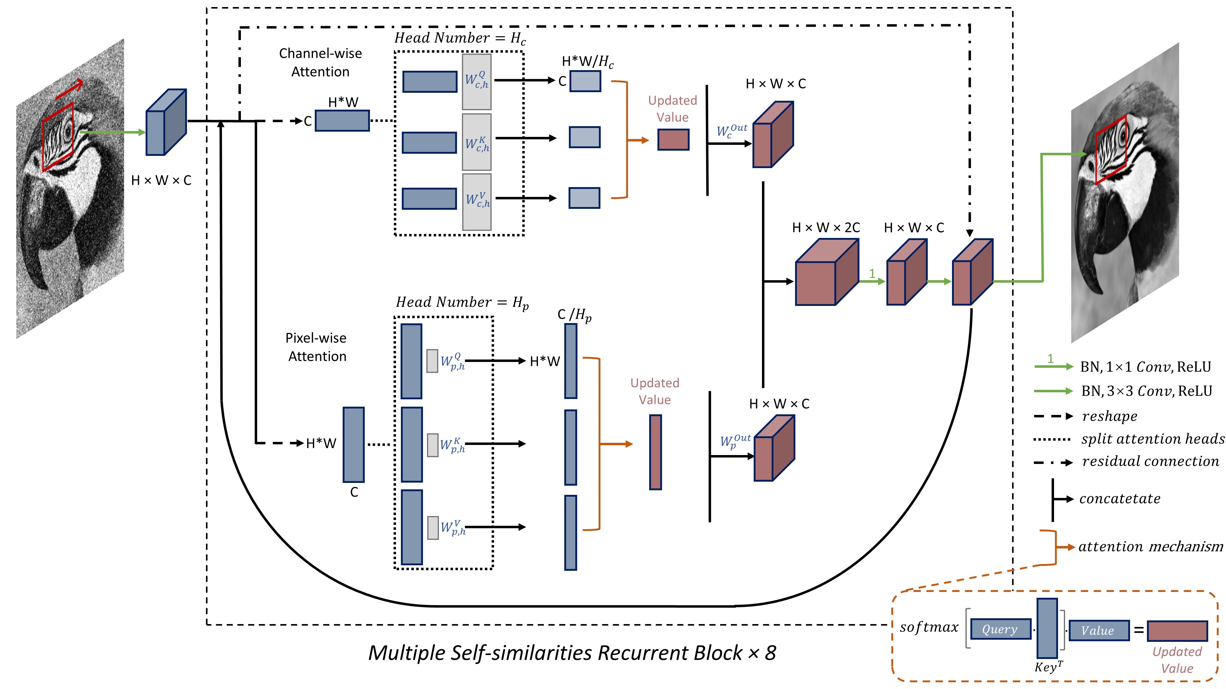
Figure 1: An illustration of the proposed MSSN denoiser. Each input patch is obtained from the noisy image stride by stride. After the first convolutional layer, the features are subsequently processed with 8 recurrent blocks. Each recurrent block has dedicated channel-wise and pixel-wise attention layers consisting of multiple heads in order to capture different types of complex relationships. Then two convolutional layers are used for mixing updated features. The final denoised patch is obtained by another convolutional layer.

2 Background

In order to solve (1) in the context of imaging inverse problems, APGM is widely adopted to avoid the differentiation of the non-smooth $h$. Recently, Kamilov et al. [27] proposed a PnP algorithm based on APGM by replacing the proximal operator with a general denoising function. Algorithm 1 summarizes the PnP-APGM, where $\nabla g$ is the gradient of $g$, $\gamma$ is the step size, and sequence $\{q_{k}\}$ are used to accelerate PGM [9]. The key advantage of PnP-APGM is that it regularizes the reconstruction by using advanced off-the-shelf denoisers. Similar PnP algorithms have also been developed using ADMM [34], approximate message passing (AMP) [35], Newtons method [36], and online processing [31]. Denoiser priors have also been used within an alternative framework called regularization by denoising (RED) [37, 38, 39, 40].

Different denoisers have been adopted within PnP including BM3D [14, 41, 42, 43, 19, 20, 27, 25, 44, 45, 31], sparse representations [21], non-local means (NLM) [19, 46, 47], Gaussian mixture models [22, 24, 48], and deep-learning-based denoisers. Among the latter, DnCNN [18] with residual learning, FFDNet [49] with noise adaptability, and generative adversarial networks (GANs) [50] have been particularly popular within PnP [26, 51, 52, 53, 54].

This letter is based on a hypothesis that further improvements in PnP can be achieved by using learned non-local priors. In conventional denoiers, such as NLM and BM3D, non-local information is infused by jointly processing multiple image patches that are similar to a given reference patch. In deep neural networks, non-local similarities can be calculated using attention mechanisms as was recently done for image restoration in [32] and [33]. However, this prior work [32, 33] restricts the number of attention mechanisms to one, which limits the ability of the network to learn more complex non-local information. In the proposed MSSN, we use multi-head attention (MA) to exploit different types of non-local relationships among the feature maps extracted from image, thus boosting the performance of the prior.

3 Proposed Denoiser Prior

As illustrated in Fig. 1, the proposed denoiser mainly consists of two parts. The first part is a convolutional layer which convolves a noisy patch to produce 128 feature maps. The second part consists of 8 recurrent blocks for capturing the non-local relationships among the feature maps. Each block is composed of one multi-head self-attention layer, two convolutional layers, and a residual connection. Before each convolutional layer, batch normalization is added. Each convolutional kernel is $3\times 3$ and ReLU activations are used across the whole network. Additionally, our denoiser uses the residual learning [55] technique to predict the noise of the input patch.

Algorithm 1 PnP-APGM

0:  $\bm{x}^{0}=\bm{s}^{0}\in\mathbb{R}^{n},\gamma>0,\sigma>0,\{q_{k}\}_{k\in\mathbb{N}}$

1:  for $k=1,2,...$ do

2:     $\bm{z}^{k}\leftarrow\bm{s}^{k-1}-\gamma\nabla g(\bm{s}^{k-1})$

3:     $\bm{x}^{k}\leftarrow\text{denoise}_{\sigma}(\bm{z}^{k-1})$

4:     $q_{k}\leftarrow\frac{1}{2}(1+\sqrt{1+4q^{2}_{k-1}})$

5:     $\bm{s}^{k}\leftarrow\bm{x}^{k}+((q_{k-1}-1)/q_{k})(\bm{x}^{k}-\bm{x}^{k-1})$

6:  end for

Multi-head attention (MA) in our neural network is the core part that captures the complex relationship among the feature maps. Attention mechanism is widely used for natural language processing (NLP) to estimate the correlation between two sequences. Similarly, it has the potential to capture the relationships between two feature maps when we regard each row of the feature map as a sequence. Moreover, MA is able to represent different types of complex relationships while a single attention mechanism learns more simple relationships. In the proposed denoiser, MA is extended into two types to make the full use of non-local information. The first is the pixel-wise attention and the second is the channel-wise attention.

Given a latent representation in terms of keys and values $\bm{z}=[\bm{z}_{1},\bm{z}_{2},...,\bm{z}_{n}]$ , and a query vector $\bm{q}$, attention calculates the alignment or similarity score between $\bm{q}$ and $\bm{z}_{i}$ (position $i$ of keys) through a function $\theta(\bm{q},\bm{z}_{i})$. The softmax function normalizes all of the scores $[\theta(\bm{q},\bm{z}_{i})]_{i=1}^{n}$ to a probability distribution as

$$\textsf{softmax}(\theta(\bm{q},\bm{z}))_{i}=\frac{e^{\theta(\bm{q},\bm{z}_{i})}}{\sum_{j=1}^{n}e^{\theta(\bm{q},\bm{z}_{j})}}\;,\;\;\;\;i=1,2,...,n.$$ (2)

The updated value of $\bm{q}$ is calculated as $\sum_{i=1}^{n}\textsf{softmax}(\theta(\bm{q},\bm{z})_{i})\bm{z}_{i}$. Dot-product $\theta(\bm{q},\bm{z}_{i})=\bm{q}^{\mathsf{T}}\bm{z}_{i}$ is widely used as the function $\theta$. Note that the attention mechanism makes it easier to learn long range dependencies due to the direct comparison between $\bm{z}_{i}$ and $\bm{q}$. This $\mathcal{O}(1)$ path length of the attention mechanism makes it preferable to the $\mathcal{O}(n)$ path length of using traditional RNN processing. Additionally, for self-attention $\bm{q}$ is replaced by $\bm{z}_{p}$ to compute the weight distribution between different positions of latent representations $\bm{z}_{p}$ and $\bm{z}_{i}$. In 2D scenario, the formula of self-attention becomes

$$\textsf{Attention}(\textsf{Query},\textsf{Key},\textsf{Value})=\textsf{softmax}(\textsf{Query}\textsf{Key}^{\mathsf{T}})\textsf{Value},$$ (3)

where Query, Key and Value are all latent representations $\bm{z}\in\mathbb{R}^{m\times n}$.

Furthermore, multi-head attention is used to capture different types of dependencies between sequences.

$$\textsf{MultiHeadAttention}(\textsf{Query},\textsf{Key},\textsf{Value})=[\textsf{head}_{1},...,\textsf{head}_{h}]W^{Out},$$ (4)

where $\textsf{head}_{h}=\textsf{Attention}(\textsf{Query}W^{Q}_{h},\textsf{Key}W^{K}_{h},\textsf{Value}W^{V}_{h})$, matrices $W^{Q}_{h}\in\mathbb{R}^{n\times d_{k}}$, $W^{K}_{h}\in\mathbb{R}^{n\times d_{k}}$ and $W^{V}_{h}\in\mathbb{R}^{n\times d_{v}}$ map Query, Key and Value into lower dimensional spaces $h$ times, to reduce computational cost when we create several attention heads. After applying Attention, we concatenate the ouputs and pipe through a linear layer $W^{Out}\in\mathbb{R}^{hd_{v}\times n}$. In this way, the model can jointly process information from different representation sub-spaces at different positions which improves the capability of matching complex relationships among features.

Our MSSN denoiser adopts this mechanism to exploit potential dependencies in an image. Specifically, we divide the attention mechanism into pixel-wise and channel-wise attention layers. In channel-wise attention, queries, keys, and values are generated by $W^{Q}_{c,h}\in\mathbb{R}^{n\times d_{k}}$, $W^{K}_{c,h}\in\mathbb{R}^{n\times d_{k}}$ and $W^{V}_{c,h}\in\mathbb{R}^{n\times d_{v}}$ from the reshaped feature maps $\bm{z}\in\mathbb{R}^{C\times HW}$ along the spatial axis in each attention head. The computation of matrix multiplication in $\textsf{Attention}(\textsf{Query},\textsf{Key},\textsf{Value})$ function simply compares the similarity between Query and Key in the same spatial position but different channels. Then the updated values are obtained as in eq. (3). Similarly, in pixel-wise attention, queries, keys, and values are generated by $W^{Q}_{p,h}\in\mathbb{R}^{n\times d_{k}}$, $W^{K}_{p,h}\in\mathbb{R}^{n\times d_{k}}$ and $W^{V}_{p,h}\in\mathbb{R}^{n\times d_{v}}$ from $\bm{z}\in\mathbb{R}^{HW\times C}$ along the channel axis in each attention head. Similarities of feature maps in the same channel, but in different spatial positions are calculated. Lastly, we concatenate the updated pixel-wise and channel-wise values obtained by $W_{p}^{Out}\in\mathbb{R}^{hd_{v}\times n}$ and $W_{c}^{Out}\in\mathbb{R}^{hd_{v}\times n}$, then dimension reduction is done using another $1\times 1$ convolutional layer. The mixed attention values are obtained in the same shape of the input feature maps.

Table 1: Average SNRs of MR Image Reconstruction for Randomly Selected Samples

	IFFT	TV	BM3D	DnCNN	DnCNN (MRI)	SSN	MSSN
36 Lines	17.36	20.03	20.62	19.15	20.17	21.01	21.18
48 Lines	18.54	21.27	21.84	20.58	21.37	21.71	22.03

4 Experiments

We validate the proposed denoiser within PnP-APGM for MRI reconstruction by comparing it with three popular priors: total variation (TV) [1], BM3D [15], and DnCNN [18]. Specifically, we reconstruct from the subsampled $k$-space measurements $\bm{y}$ and the data-fidelity term in eq. (1) becomes

$$g(\bm{x})=\frac{1}{2}\lVert\bm{y}-\mathcal{S}\circ\mathcal{F}(\bm{x})\rVert_{2}^{2}\;,$$ (5)

where $\mathcal{F}$ denotes the Fourier transform, $\mathcal{S}$ is subsampling, and $\circ$ denotes the composition. We use 10 randomly-picked samples from the open-source fastMRI dataset [56] for testing.

4.1 Experimental Settings

To test the robustness of our MSSN denoiser as a PnP prior, we trained it on natural images from the standard BSD500 dataset, but tested it on MRI images. MSSN is trained on patches of size $42\times 42$ using the Gaussian noise with $\sigma=5$. The number of recurrent blocks is 8 and the number of features for each $3\times 3$ convolutional kernel is set to 128 across all the network. The number of heads for both types of attention (pixel-wise and channel-wise) are set to 2. Adam algorithm is adopted to optimize the neural network by minimizing the mean square error (MSE) loss. The learning rate starts at $10^{-3}$, then decreases by half every $5\times 10^{4}$ iterations with the epoch number of 80.

Radial sampling method in $k$-space is used for acquisition. We used highly compressive 36 and 48 lines in our experiments. We optimized the hyperparameters of TV and BM3D for SNR. We provided comparisons with two variants of DnCNN, one trained on the same set of natural images as MSSN and the other trained specifically on the fastMRI dataset (labeled as DnCNN (MRI)). Both DnCNN denoisers were trained with noise $\sigma=5$ For better comparison between the proposed mixed multi-head attention and single attention in the RNN denoiser, these two attention mechanisms are tested (referred as MSSN and SSN, respectively).

4.2 Results and Discussions

The quantitative results in Table 1 show that MSSN outperforms the optimized conventional regularizer TV, BM3D, and DnCNN denoisers. MSSN achieves the highest average SNR of 21.18 dB when using 36-lines $k$-space subsampling and 22.03 dB when using 48 lines. The SSN denoiser is competitive with BM3D without using the mixed multi-head attention. The MSSN denoiser further improves the reconstruction performance compared to SSN, and results in the lowest reconstruction error, even when trained on natural images.

Figure 2 demonstrates the details of the MRI reconstruction. The first two rows are the reconstruction results of no. 58 in fastMRI dataset using 36-lines and 48-lines radial sampling respectively. The last two rows are results of no. 21119. Visual inspection of reconstructed images reveals that proposed denoiser is robust in these two T1, T2-weighted MR images of bones, and artefacts are diminished using SSN or MSSN denoiser compared to conventional denoisers. More crucially, PnP algorithm using MSSN keeps subtle yet important anatomical details and offers more faithful reconstructions that can be recognized in the zoomed-in views.

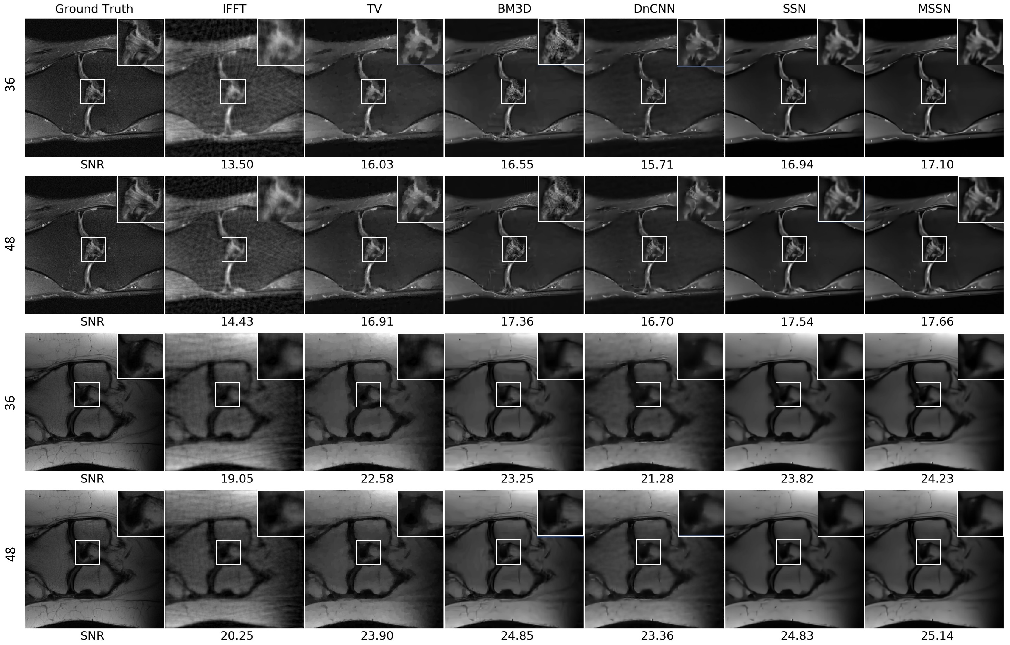
Figure 2: Illustrations of MRI reconstruction from $k$-space downsampled data (no. 58 and no. 21119 using radial sampling, the first and third rows use 36 lines for sampling and the second and the fourth rows use 48 lines) using different denoisers within PnP. Each reconstruction is labeled with its SNR (dB) value with respect to the ground truth.

5 Conclusion

In this letter, we proposed and validated a new PnP denoiser called MSSN, bringing together two concepts, namely RNN and MA. MSSN captures multiple self-similarities of non-local features. We combined MSSN with PnP-APGM for solving an inverse problem in MRI. Experimental results on fastMRI dataset show that MSSN improves both quantitative and perceptual quality, even when trained on natural images. This suggests that the powerful feature extraction of deep RNN and the ability to capture complex non-local relationships of the MA mechanism (in both pixel-wise and channel-wise attention) makes MSSN competitive with the state-of-the-art PnP priors.

References

- [1] L. I. Rudin, S. Osher, and E. Fatemi, “Nonlinear total variation based noise removal algorithms,” Physica D, vol. 60, no. 1-4, pp. 259–268, 1992.
- [2] M. A. Figueiredo and R. D. Nowak, “Wavelet-based image estimation: an empirical bayes approach using Jeffrey’s noninformative prior,” IEEE Trans. Image Process., vol. 10, no. 9, pp. 1322–1331, 2001.
- [3] M. Elad and M. Aharon, “Image denoising via sparse and redundant representations over learned dictionaries,” IEEE Trans. Image Process., vol. 15, no. 12, pp. 3736–3745, 2006.
- [4] A. Danielyan, V. Katkovnik, and K. Egiazarian, “BM3D frames and variational image deblurring,” IEEE Trans. Image Process., vol. 21, no. 4, pp. 1715–1728, 2011.
- [5] N. Parikh, S. Boyd et al., “Proximal algorithms,” Foud. Trends Optim., vol. 1, no. 3, pp. 127–239, 2014.
- [6] M. A. Figueiredo and R. D. Nowak, “An EM algorithm for wavelet-based image restoration,” IEEE Trans. Image Process., vol. 12, no. 8, pp. 906–916, 2003.
- [7] I. Daubechies, M. Defrise, and C. De Mol, “An iterative thresholding algorithm for linear inverse problems with a sparsity constraint,” Commun. Pure Appl. Math., vol. 57, no. 11, pp. 1413–1457, 2004.
- [8] J. Bect et al., “A -unified variational framework for image restoration,” in Eur. Conf. Comput. Vision. Springer, 2004, pp. 1–13.
- [9] A. Beck and M. Teboulle, “Fast gradient-based algorithms for constrained total variation image denoising and deblurring problems,” IEEE Trans. Image Process., vol. 18, no. 11, pp. 2419–2434, 2009.
- [10] J. Eckstein and D. P. Bertsekas, “On the Douglas—Rachford splitting method and the proximal point algorithm for maximal monotone operators,” Math. Program., vol. 55, no. 1-3, pp. 293–318, 1992.
- [11] M. V. Afonso, J. M. Bioucas-Dias, and M. A. Figueiredo, “Fast image recovery using variable splitting and constrained optimization,” IEEE Trans. Image Process., vol. 19, no. 9, pp. 2345–2356, 2010.
- [12] M. K. Ng, P. Weiss, and X. Yuan, “Solving constrained total-variation image restoration and reconstruction problems via alternating direction methods,” SIAM J. Sci. Comput., vol. 32, no. 5, pp. 2710–2736, 2010.
- [13] S. Boyd et al., “Distributed optimization and statistical learning via the alternating direction method of multipliers,” Found. Trends Mach. Learn., vol. 3, no. 1, pp. 1–122, 2011.
- [14] S. V. Venkatakrishnan, C. A. Bouman, and B. Wohlberg, “Plug-and-play priors for model based reconstruction,” in IEEE Global Conf. Signal Inf. Process. IEEE, 2013, pp. 945–948.
- [15] K. Dabov et al., “Image denoising by sparse 3-D transform-domain collaborative filtering,” IEEE Trans. Image Process., vol. 16, no. 8, pp. 2080–2095, Aug 2007.
- [16] S. Gu et al., “Weighted nuclear norm minimization with application to image denoising,” in IEEE Conf. Comput. Vision Pattern Recognit., 2014, pp. 2862–2869.
- [17] Y. Chen and T. Pock, “Trainable nonlinear reaction diffusion: A flexible framework for fast and effective image restoration,” IEEE Trans. Pattern Anal. Mach. Intell., vol. 39, no. 6, pp. 1256–1272, 2016.
- [18] K. Zhang et al., “Beyond a Gaussian denoiser: Residual learning of deep CNN for image denoising,” IEEE Trans. Image Process., vol. 26, no. 7, pp. 3142–3155, 2017.
- [19] S. Sreehari et al., “Plug-and-play priors for bright field electron tomography and sparse interpolation,” IEEE Trans. Comput. Imaging, vol. 2, no. 4, pp. 408–423, 2016.
- [20] S. H. Chan, X. Wang, and O. A. Elgendy, “Plug-and-play ADMM for image restoration: Fixed-point convergence and applications,” IEEE Trans. Comput. Imaging, vol. 3, no. 1, pp. 84–98, 2016.
- [21] A. Brifman, Y. Romano, and M. Elad, “Turning a denoiser into a super-resolver using plug and play priors,” in IEEE Int. Conf. Image Process. IEEE, 2016, pp. 1404–1408.
- [22] A. M. Teodoro, J. M. Bioucas-Dias, and M. A. T. Figueiredo, “Image restoration and reconstruction using variable splitting and class-adapted image priors,” in IEEE Int. Conf. Image Process., Sep. 2016, pp. 3518–3522.
- [23] K. Zhang et al., “Learning deep cnn denoiser prior for image restoration,” in IEEE Conf. Comput. Vision Pattern Recognit., July 2017.
- [24] A. M. Teodoro, J. M. Bioucas-Dias, and M. A. T. Figueiredo, “Scene-adapted plug-and-play algorithm with convergence guarantees,” in IEEE Int. Workshop Mach. Learn. Signal Process., Sep. 2017, pp. 1–6.
- [25] S. Ono, “Primal-dual plug-and-play image restoration,” IEEE Signal Process. Lett., vol. 24, no. 8, pp. 1108–1112, Aug 2017.
- [26] T. Meinhardt et al., “Learning proximal operators: Using denoising networks for regularizing inverse imaging problems,” in IEEE Int. Conf. Comput. Vision, Oct 2017, pp. 1799–1808.
- [27] U. S. Kamilov, H. Mansour, and B. Wohlberg, “A plug-and-play priors approach for solving nonlinear imaging inverse problems,” IEEE Signal Process. Lett., vol. 24, no. 12, pp. 1872–1876, Dec 2017.
- [28] L. Bottou and O. Bousquet, “The tradeoffs of large scale learning,” in Adv. Neural inf. Process. Syst., 2008, pp. 161–168.
- [29] U. S. Kamilov et al., “Optical tomographic image reconstruction based on beam propagation and sparse regularization,” IEEE Trans. Comput. Imaging, vol. 2, no. 1, pp. 59–70, March 2016.
- [30] R. Ahmad et al., “Plug and play methods for magnetic resonance imaging,” arXiv preprint arXiv:1903.08616, 2019.
- [31] Y. Sun, B. Wohlberg, and U. S. Kamilov, “An online plug-and-play algorithm for regularized image reconstruction,” IEEE Trans. Comput. Imaging, pp. 1–1, 2019.
- [32] D. Liu et al., “Non-local recurrent network for image restoration,” in Adv. Neural Inf. Process. Syst., 2018, pp. 1673–1682.
- [33] Y. Zhang et al., “Residual non-local attention networks for image restoration,” arXiv preprint arXiv:1903.10082, 2019.
- [34] W. Dong, P. Wang, W. Yin, and G. Shi, “Denoising prior driven deep neural network for image restoration,” IEEE transactions on pattern analysis and machine intelligence, 2018.
- [35] C. A. Metzler, A. Maleki, and R. G. Baraniuk, “From denoising to compressed sensing,” IEEE Transactions on Information Theory, vol. 62, no. 9, pp. 5117–5144, 2016.
- [36] G. T. Buzzard, S. H. Chan, S. Sreehari, and C. A. Bouman, “Plug-and-play unplugged: Optimization-free reconstruction using consensus equilibrium,” SIAM Journal on Imaging Sciences, vol. 11, no. 3, pp. 2001–2020, 2018.
- [37] Y. Romano, M. Elad, and P. Milanfar, “The little engine that could: Regularization by denoising (RED),” SIAM J. Imaging Sci., vol. 10, no. 4, pp. 1804–1844, 2017.
- [38] E. T. Reehorst and P. Schniter, “Regularization by denoising: Clarifications and new interpretations,” IEEE Trans. Comput. Imaging, vol. 5, no. 1, pp. 52–67, 2018.
- [39] Y. Sun, J. Liu, and U. S. Kamilov, “Block Coordinate Regularization by Denoising,” arXiv preprint arXiv:1905.05113, 2019.
- [40] G. Mataev, M. Elad, and P. Milanfar, “DeepRED: Deep Image Prior Powered by RED,” arXiv preprint arXiv:1903.10176, 2019.
- [41] F. Heide et al., “FlexISP: A flexible camera image processing framework,” ACM Trans. Graph., vol. 33, no. 6, pp. 231:1–231:13, Nov. 2014.
- [42] Y. Dar et al., “Postprocessing of compressed images via sequential denoising,” IEEE Trans. Image Process., vol. 25, no. 7, pp. 3044–3058, 2016.
- [43] A. Rond, R. Giryes, and M. Elad, “Poisson inverse problems by the plug-and-play scheme,” J. Visual Commun. Image Represent., vol. 41, pp. 96–108, 2016.
- [44] X. Wang and S. H. Chan, “Parameter-free plug-and-play ADMM for image restoration,” in IEEE Int. Conf. Acoust. Speech Signal Process. IEEE, 2017, pp. 1323–1327.
- [45] Y. Sun et al., “Regularized Fourier ptychography using an online plug-and-play algorithm,” in IEEE Int. Conf. Acoust. Speech Signal Process. IEEE, 2019, pp. 7665–7669.
- [46] V. Unni, S. Ghosh, and K. N. Chaudhury, “Linearized ADMM and fast nonlocal denoising for efficient plug-and-play restoration,” in IEEE Global Conf. Signal Inf. Process. IEEE, 2018, pp. 11–15.
- [47] S. H. Chan, “Performance analysis of plug-and-play ADMM: A graph signal processing perspective,” IEEE Trans. Comput. Imaging, vol. 5, no. 2, pp. 274–286, 2019.
- [48] M. Shi and L. Feng, “Plug-and-play prior based on Gaussian mixture model learning for image restoration in sensor network,” IEEE Access, vol. 6, pp. 78 113–78 122, 2018.
- [49] K. Zhang, W. Zuo, and L. Zhang, “FFDNet: Toward a fast and flexible solution for CNN based image denoising,” vol. 27, no. 9. IEEE, 2018, pp. 4608–4622.
- [50] I. Goodfellow et al., “Generative adversarial nets,” in Adv. Neural Inf. Process. Syst., 2014, pp. 2672–2680.
- [51] D. H. Ye et al., “Deep residual learning for model-based iterative ct reconstruction using plug-and-play framework,” in IEEE Int. Conf. Acoust. Speech Signal Process. IEEE, 2018, pp. 6668–6672.
- [52] T. Tirer and R. Giryes, “Image restoration by iterative denoising and backward projections,” IEEE Trans. Image Process., vol. 28, no. 3, pp. 1220–1234, 2018.
- [53] E. K. Ryu et al., “Plug-and-play methods provably converge with properly trained denoisers,” arXiv preprint arXiv:1905.05406, 2019.
- [54] K. Zhang, W. Zuo, and L. Zhang, “Deep plug-and-play super-resolution for arbitrary blur kernels,” in IEEE Conf. Comput. Vision Pattern Recognit., 2019, pp. 1671–1681.
- [55] K. He et al., “Deep residual learning for image recognition,” in IEEE Conf. Comput. Vision Pattern Recognit., 2016, pp. 770–778.
- [56] J. Zbontar et al., “fastMRI: An open dataset and benchmarks for accelerated MRI,” 2018.