Direct numerical simulation of high-pressure mixing in turbulent jets

Abstract

Combustion in automotive and aerospace applications employing diesel, gas turbine and liquid rocket engines is preceded by injection and mixing of fuel and oxidizer at high pressures, often exceeding mixture critical values. Experimental observations indicate that the jets injected at supercritical pressures exhibit significantly different dynamics than the jets at subcritical conditions, owing to the lack of distinct liquid and gas phases in supercritical state. As a result, the averaged flow quantities such as the potential core length, jet spatial growth rate and velocity decay profiles differ in the two conditions, resulting in different mixed-fluid distributions. In this study, turbulent jet direct numerical simulations (DNS) are performed to examine the variations in statistics between injection of Nitrogen ($\mathrm{N_{2}}$) in Nitrogen ($\mathrm{N_{2}}$) at subcritical (perfect-gas) and supercritical conditions. Isothermal round jets at Reynolds number ($Re_{D}$), based on jet diameter ($D$) and jet orifice velocity ($U_{0}$), of $5000$ and Mach number of $0.6$ are considered. For mixing analyses, a passive scalar transported with the flow is examined.

1 Introduction

Fuel injection and turbulent mixing at supercritical pressures determines ignition and combustion in numerous engineering applications. Flow evolution under such conditions is characterized by strong non-linear coupling between dynamics, transport coefficients, and thermodynamics. A model that accounts for these non-linear effects in computation of the thermodynamic state of the mixture, and the heat and mass fluxes in a multi-component fluid-flow simulation was proposed by Masi et al. [1]. The goal of the present study is to evaluate the model in a turbulent free-jet configuration to simulate fuel injection and mixing in high-pressure($p$) combustion chambers of propulsion systems.

Validation of numerical simulations at high-$p$ conditions, where theoretical results are scarce, requires comparisons with experimental data. However, most experimental studies (e.g., [2, 3, 4]) inject liquid (fuel at subcritical conditions) or high-density fluid (fuel at supercritical conditions) at high Reynolds numbers ($Re_{D}\geq 20,000$), and provide qualitative visual information about flow dynamics and mixing. A numerical simulation of these flows, for direct comparisons with the experiments, would require several models. For example, models to accommodate potential two-phase/density-jump regions and to account for the subgrid-scale fluxes would be required, in addition to the thermodynamic model. Moreover, appropriate inflow and boundary treatments that accurately replicate the experimental conditions are also imperative. Interactions between the models and numerical details make validation of individual models infeasible in such complex flows at high-$Re_{D}$. Moreover, the lack of quantitative turbulence/mixing statistics measurements in high-$p$ experiments makes assessment of a model even more challenging.

To mitigate the model interactions, direct numerical simulations at $Re_{D}$ of $5,000$ are considered in this study. Jet flow at perfect-gas conditions, for which theoretical [5, 6] and experimental [7, 8] results exist, is first considered to validate the numerical setup and to create a database for flow-behavior comparisons against multicomponent flows at high pressures. To systematically initiate the study, mixing behavior in the single-species flows is assessed by a virtual passive scalar transported with the flow, modeling diffusion at unity Schmidt number ($Sc$) justifiable under perfect-gas conditions.

Accurate turbulent free-jet flow computation requires a careful choice of inflow/boundary conditions, domain size, and numerical discretization. The near-field jet flow evolution is particularly sensitive to the choice of inflow perturbations, and several studies [9, 10] have examined its influence on turbulence statistics. The jet flow attains self-similarity after the development region, containing potential core collapse and transition to turbulence; the axial distance to attain a self-similar state depends on the inflow perturbations. Moreover, theoretical results [11] suggest that the self-similar state may also depend on the inflow, requiring the similarity variables to be appropriately modified for analyses. Although the theoretical and experimental jet flow studies focus on the flow statistics in the self-similar region, in practical applications with small combustion chambers, the jet near-field is equally important because this is where the phenomena determining the flame occur, and this is where control must be exercised to influence flow behavior.

2 Governing equations

For the single-species flow of interest here, the conservation equations solved in this study are:

$$\frac{\partial\rho}{\partial t}+\frac{\partial}{\partial x_{j}}\left[\rho u_{j}\right]=0,$$ (1)

$$\frac{\partial}{\partial t}\left(\rho u_{i}\right)+\frac{\partial}{\partial x_{j}}\left[\rho u_{i}u_{j}+p\delta_{ij}-\sigma_{ij}\right]=0,$$ (2)

$$\frac{\partial}{\partial t}\left(\rho e_{t}\right)+\frac{\partial}{\partial x_{j}}\left[\left(\rho e_{t}+p\right)u_{j}-u_{i}\sigma_{ij}+q_{j}\right]=0,$$ (3)

$$\frac{\partial}{\partial t}\left(\rho\xi\right)+\frac{\partial}{\partial x_{j}}\left[\rho\xi\ u_{j}+J_{j}\right]=0,$$ (4)

where $t$ denotes the time, $x$ is a Cartesian coordinate, subscripts $i$ and $j$ refer to the spatial coordinates, $u_{i}$ is the velocity, $p$ is the pressure, $\delta_{ij}$ is the Kronecker delta, $e_{t}=e+u_{i}u_{i}/2$ is the total energy (i.e., internal energy, $e$, plus kinetic energy), $\xi\in\left[0,1\right]$ is a virtual passive scalar transported with the flow, $\sigma_{ij}$ is the Newtonian viscous stress tensor

$$\sigma_{ij}=\mu\left(2S_{ij}-\dfrac{2}{3}S_{kk}\delta_{ij}\right),\text{ \ \ }S_{ij}=\dfrac{1}{2}\left(\dfrac{\partial u_{i}}{\partial x_{j}}+\dfrac{\partial u_{j}}{\partial x_{i}}\right),$$ (5)

where $\mu$ is the viscosity, $S_{ij}$ is the strain-rate tensor, and $q_{j}=-\lambda\thinspace\partial T/\partial x_{j}$ and $J_{j}=-\mathscr{D}\thinspace\partial\xi/\partial x_{j}$ are the $j$-direction heat flux and scalar diffusion flux, respectively. $\lambda$ is the thermal conductivity and $\mathscr{D}=\mu/Sc$ is the scalar diffusivity, where $Sc$ denotes the Schmidt number. The injected fluid is assigned a scalar value of 1, whereas the chamber fluid a value of 0.

Two jet-flow simulations at conditions summarized in Table 1 are performed to examine flow statistics differences between injection at perfect-gas and supercritical conditions. Only the chamber pressure $p_{\infty}$ differs between the two cases.

For the near-atmospheric-$p$ simulation (Case 1), the perfect gas equation of state is applicable, given by

$$p=\frac{\rho R_{\mathrm{u}}T}{m},$$

where $R_{u}$ is the universal gas constant and $m$ is the species molar mass. The viscosity is modeled as a power law

$$\mu=\mu_{R}\left(\frac{T}{T_{R}}\right)^{n}$$

with $n=2/3$ and the reference viscosity $\mu_{R}=\rho_{0}U_{0}D/Re_{D}$, where $\rho_{0}$ and $U_{0}$ are the jet-exit fluid density and velocity, respectively, and the reference temperature $T_{R}=293\thinspace\mathrm{K}$. The thermal conductivity $\lambda=\mu C_{p}/\mathrm{Pr}$, where Prandtl number $\mathrm{Pr}=0.7$, the ratio of specific heats $\gamma=1.4$, and the isobaric heat capacity $C_{p}=\gamma R_{\mathrm{u}}/\left(\gamma-1\right)$ is assumed.

For the high-$p$ simulation (Case 2), the governing equations (1)-(4) are closed using the Peng-Robinson (PR) equation of state (EOS)

$$p=\frac{R_{\mathrm{u}}T}{\left(v_{\mathrm{PR}}-b_{\mathrm{mix}}\right)}-\frac{a_{\mathrm{mix}}}{\left(v_{\mathrm{PR}}^{2}+2b_{\mathrm{mix}}v_{\mathrm{PR}}-b_{\mathrm{mix}}^{2}\right)},$$

where the pressure, $p$, and temperature, $T$, are obtained as an iterative solution from the density, $\rho$, and internal energy, $e$, obtained from the conservation equations [12]. The molar PR volume $v_{\mathrm{PR}}=v-v_{\mathrm{s}}$, where the molar volume $v=m/\rho$. $v_{\mathrm{s}}$ denotes the volume shift introduced to improve the accuracy of the PR EOS at high pressures [12, 13]. $a_{\mathrm{mix}}$ and $b_{\mathrm{mix}}$ are obtained from the expressions detailed in [14, Appendix B].

The physical viscosity, $\mu_{\mathrm{ph}}$, and thermal conductivity, $\lambda_{\mathrm{ph}}$, are calculated using the Lucas method [15, Chapter 9] and the Stiel-Thodos method [15, Chapter 10], respectively. The computational viscosity, $\mu$, and thermal conductivity, $\lambda$, are then obtained by scaling $\mu_{\mathrm{ph}}$ and $\lambda_{\mathrm{ph}}$ with factor $\mathcal{F}=\mu_{R}/\mu_{\mathrm{ph},0}$, i.e., $\mu=\mathcal{F}\mu_{\mathrm{ph}}$ and $\lambda=\mathcal{F}\lambda_{\mathrm{ph}}$, to simulate the flow at a specified Reynolds number $Re_{D}$. The inflow physical viscosity, $\mu_{\mathrm{ph},0}$, is obtained from the Lucas method using the pressure $p_{\infty}$ and the average temperature $\left(T_{\mathrm{inj}}+T_{\mathrm{ch}}\right)/2$, where the subscripts “$\mathrm{inj}$” and “$\mathrm{ch}$” denote the injection and chamber conditions, respectively.

To examine the robustness of the above EOS and transport coefficient models at supercritical conditions, Figure 1 compares the density, isobaric heat capacity, and the transport coefficients $\mu_{\mathrm{ph}}$ and $\lambda_{\mathrm{ph}}$ obtained from the models against the National Institute of Standards and Technology (NIST) database [16] for $\mathrm{N_{2}}$ at a pressure of 50 bar and temperatures ranging from 100 K to 400 K. The supercritical temperature ($T_{c}$) of Nitrogen is 126.2 K. The transport coefficient models are accurate only at supercritical temperatures and, thus, the comparison only spans values of $T>T_{c}$. As evident, the models have good agreement with the NIST database, showing their validity at high-$p$ conditions encountered during Case 2 simulation. Figure 2 shows the compressibility factor ($Z$), indicating deviation from perfect-gas behavior, of pure Nitrogen for a temperature range at $50$ bar pressure. The compressibility factor at chamber conditions in Case 2 is $0.994$.

Case	$N_{x}\times N_{y}\times N_{z}$	$p_{\infty}$	$T_{\mathrm{ch}}$	$T_{\mathrm{inj}}$	Number of	$Re_{D}$	$Ma_{0}$	Inflow velocity
		(bar)	(K)	(K)	species			perturbation amplitude
1 (atmP)	$320\times 288\times 288$	1	293	293	1 ($\mathrm{N_{2}}$)	5000	0.6	$0.004U_{0}$
2 (highP)	$320\times 288\times 288$	50	293	293	1 ($\mathrm{N_{2}}$)	5000	0.6	$0.004U_{0}$

Table 1: Summary of the conditions for the numerical simulations.

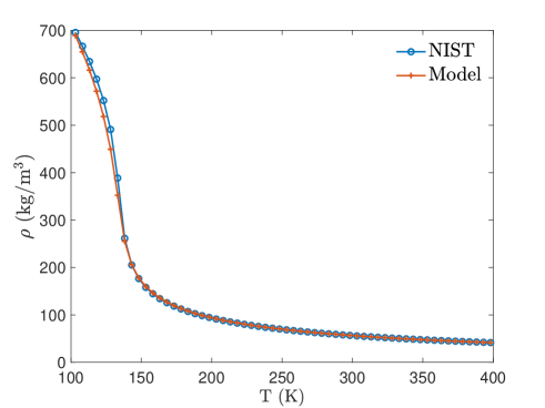
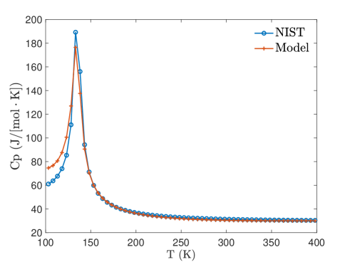
(a)                    (b)

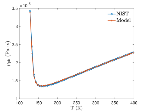
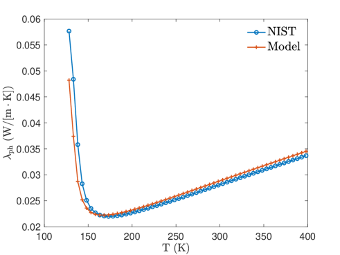
(c)                    (d)

Figure 1: EOS and transport coefficients model comparison against NIST database for pure Nitrogen at $50$ bar pressure. (a) Density, (b) Isobaric heat capacity, (c) Viscosity, and (d) Thermal conductivity.

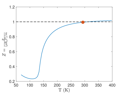
Figure 2: Compressibility factor of $\mathrm{N_{2}}$ at $50$ bar pressure. Red marker denotes the chamber conditions for Case 2.

3 Numerical details

The spatial derivatives are approximated using the sixth-order compact finite-difference scheme and time integration uses the explicit fourth-order Runge-Kutta method. The outflow boundary in axial direction and all lateral boundaries have sponge zones[17] with subsonic non-reflecting outflow Navier-Stokes characteristic boundary conditions (NSCBC)[18] at the boundary faces. Sponge zones at each outflow boundary have a width of $10\%$ of the domain length normal to the boundary face. The sponge strength at each boundary decreases quadratically with distance normal to the boundary. The performance of one-dimensional NSCBC[18] as well as its three-dimensional extension[19] by inclusion of transverse terms were also evaluated without the sponge zones; they permit occasional spurious reflections into the domain, therefore, the use of sponge zones was deemed necessary. To avoid unphysical accumulation of energy at the highest wavenumber, resulting from the non-dissipative spatial discretization, the conservative variables are filtered every five time steps using an eighth-order filter.

The computational domain extends to $42D_{0}$ in the axial ($x$-)direction and $20D_{0}$ in the $y$- and $z$-direction including the sponge zones, as shown in Figure 3. $320\times 288\times 288$ grid points are used in the $x\times y\times z$ direction, which is twice the number of grid points in each direction used for DNS by Boersma[20] at similar conditions as Case 1.

The axial grid resolution is chosen to resolve all spatial scales overwhelmingly responsible for the dissipation. Following the approach outlined in [21], for a $Re_{D}=5000$ jet simulation, the Kolmogorov length scale $\eta_{K}=0.0041\left(x-x_{0}\right)$, where $x_{0}$ denotes the virtual origin. A stretched grid designed accordingly is used for present simulations. Grid stretching is accounted for by solving the governing equations in generalized coordinates [22, 23].

The velocity profile at the jet inflow plane is given by[6]

$$u(r)=\frac{U_{0}}{2}\left(1-\tanh\left[\frac{r-r_{0}}{2\theta_{0}}\right]\right),$$

where the jet exit radius $r_{0}=D/2$ and the momentum thickness $\theta_{0}=0.04r_{0}$ is assumed. The Mach number $Ma_{0}=U_{0}/c_{\infty}=0.6$ is specified, where $c_{\infty}$ denotes the speed of sound at ambient conditions. Random perturbations with maximum amplitudes of $0.004U_{0}$ are superimposed on the inflow velocity profile to trigger jet flow transition to turbulence. No perturbations are added to fields other than velocity.

(a)

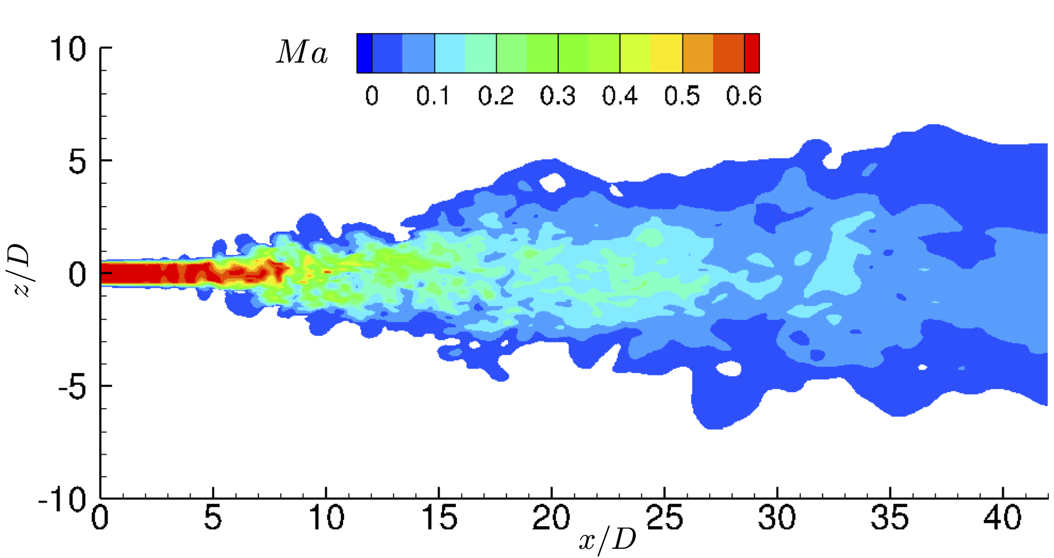
(b)

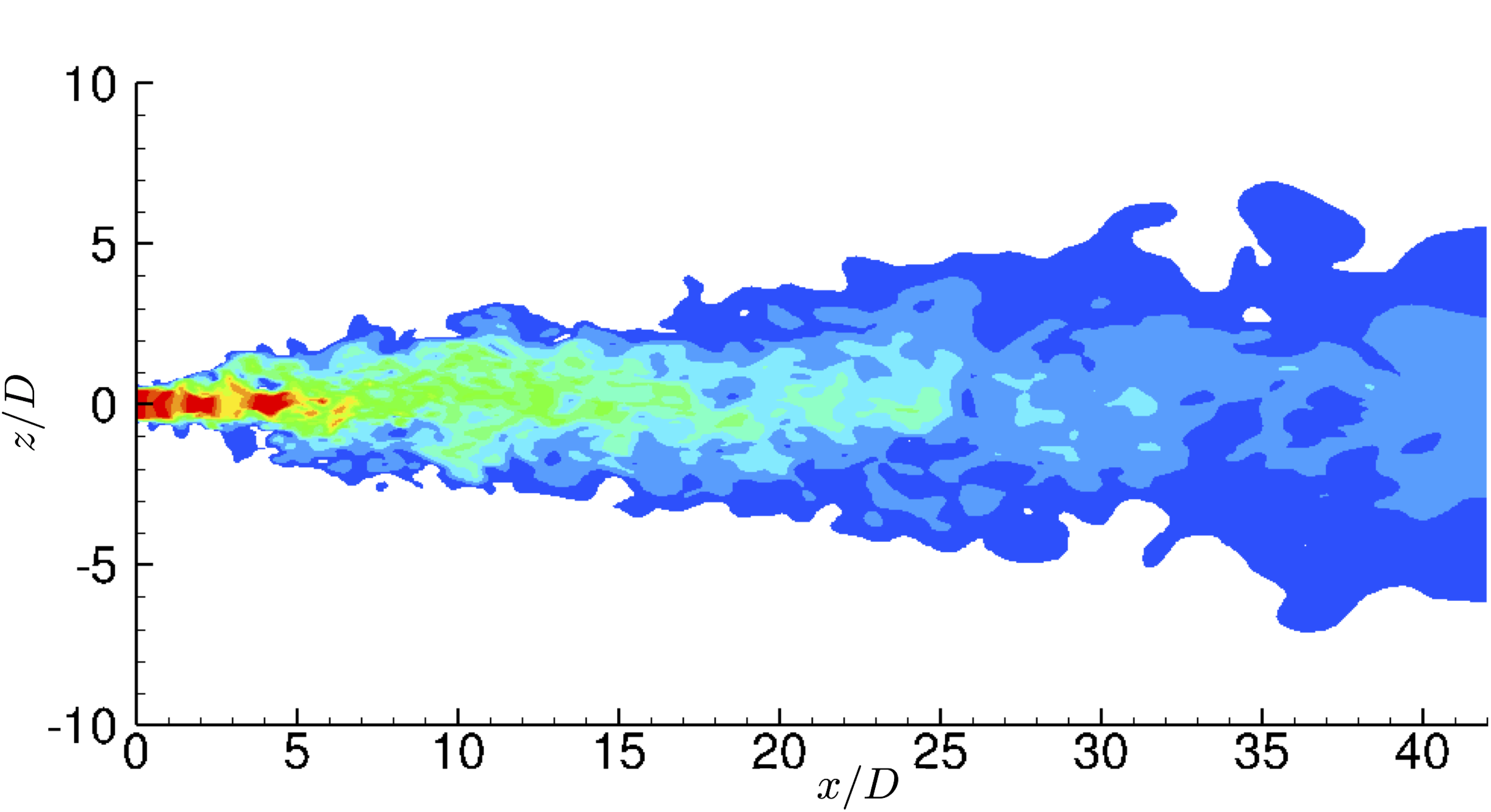
Figure 3: Instantaneous Mach number ($Ma$) field at $tU_{0}/D\approx 2500$ in (a) Case 1 and (b) Case 2. Only values of $Ma\geq 0.01$ are rendered. Legend is the same for both plots.

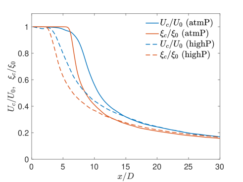
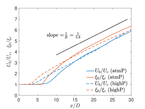
(a)                    (b)

Figure 4: Case 1 and 2 comparison showing (a) the time-averaged centerline velocity ($U_{c}$) and scalar ($\xi_{c}$) values normalized with the jet exit values $U_{0}$ and $\xi_{0}$ as a function of axial distance and (b) the inverse of the time-averaged centerline values showing linear decay asymptotically with axial distance.

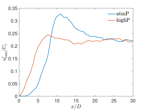
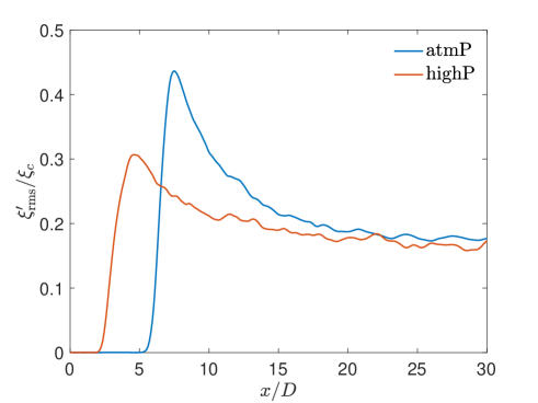
(a)                    (b)

Figure 5: Centerline root-mean-square (a) axial velocity and (b) scalar fluctuation comparison between Case 1 and 2.

4 Jet flow results and discussion

Table 1 summarizes the conditions for the numerical simulations considered in this study. In both cases, the injected and chamber fluid temperatures and pressures are the same, therefore, the jet injects into a chamber that is as dense as the injected fluid. In other words, Case 1 and 2 represent jets at same temperature and exit velocity, but in Case 1 a near-atmospheric pressure jet is injected into similar chamber conditions and in Case 2 a $50$ bar pressure jet is injected into similar chamber conditions. Physically, if the former jet has a $Re_{D}$ of 5000, the latter jet, based on the density and viscosity at $50$ bar pressure and same exit velocity $U_{0}$ and diameter $D$ as the velocity and length scale, will have $Re_{D}\sim 240,000$. A DNS at such $Re_{D}$ is infeasible, therefore, in this study $Re_{D}$ is fixed to 5000 for both cases; the $Re_{D}=5000$ condition is enforced using a computational viscosity $\mu$ that is calculated by scaling the physical viscosity by a factor $\mathcal{F}$, as discussed in Section 2.

$\mathcal{F}\approx 6.5$ ($\mu_{R}=\rho_{0}U_{0}D/Re_{D}=1.136\times 10^{-4}\thinspace\mathrm{Pa.s}$ and $\mu_{\mathrm{ph},0}=1.757\times 10^{-5}\thinspace\mathrm{Pa.s}$) for Case 1, near atmospheric pressure, and $\mathcal{F}\approx 309.4$ ($\mu_{R}=5.715\times 10^{-3}\thinspace\mathrm{Pa.s}$ and $\mu_{\mathrm{ph},0}=1.847\times 10^{-5}\thinspace\mathrm{Pa.s}$) for Case 2 at 50 bar pressure. The factor $\mathcal{F}$ is higher in Case 2 because of the higher density $\rho_{0}$ at $50$ bar that requires a higher $\mu_{R}$ for a given Reynolds number $Re_{D}$. The physical viscosity $\mu_{\mathrm{ph},0}$, on the other hand, remains relatively unchanged with increase in pressure. Simulating the two jets at same Reynolds number by using a computational viscosity, as explained above, results in the high-$p$ jet becoming unphysically more viscous than the atmospheric-$p$ jet. The following comparisons between the two cases must account for this effect.

Figure 3 shows the Mach number contours at $tU_{0}/D\approx 2500$ for both cases. The potential core is comparatively shorter in the high-$p$ case, likely due to higher computational viscosity $\mu$, from a higher value of factor $\mathcal{F}$, and resulting momentum diffusion.

Figure 4 shows the decay of time-averaged centerline velocity ($U_{c}$) and scalar concentration ($\xi_{c}$) with axial distance. For a self-similar round jet with top-hat exit velocity profile, the centerline velocity $U_{c}\left(x\right)$ is given by the empirical relation[8]

$$\frac{U_{c}\left(x\right)}{U_{0}}=\frac{B}{\left(x-x_{0}\right)/D},$$ (6)

where $B$ is a constant and $x_{0}$ denotes the virtual origin. As evident from Figure 4(b), downstream of the potential core collapse, both the time-averaged centerline velocity and scalar concentration decays as inverse of the axial distance, where the rate of decay, given by $B$, is within experimentally observed range of values [8]. The scalar concentration begins to decay upstream of velocity, consistent with the observation of Lubbers et al. [24, see Figure 6] for a passive scalar diffusing at unity Schmidt number. Despite the difference in axial location where the velocity or scalar decay begins between the near-atmospheric-$p$ and high-$p$ cases, the profiles match asymptotically with axial distance. At the time of reporting, the scalar statistics for the high-$p$ case did not fully converge; we expect the dashed red line in Figure 4 to asymptotically converge to the solid red line (like the velocity field shown in blue).

Figure 5 shows the centerline root-mean-square (r.m.s.) axial velocity and scalar concentration fluctuation, denoted by $u^{\prime}_{\mathrm{rms}}$ and $\xi^{\prime}_{\mathrm{rms}}$, respectively, normalized by the time-averaged centerline values. The centerline r.m.s. values are calculated from

$$u^{\prime}_{\mathrm{rms}}=\left(\overline{\left(u-U_{c}\right)^{2}}\right)^{1/2}=\left(\overline{u^{2}}-U_{c}^{2}\right)^{1/2}$$

and a similar expression for scalar concentration. The overbar, $\overline{\bullet}$, denotes a time average at the centerline. The r.m.s. velocity fluctuation profiles in Figure 5(a) compare favorably with the profile of Crow & Champagne [25, see Figure 13] and, similarly, the scalar fluctuation profiles in Figure 5(b) compare well with the distributions of r.m.s. scalar fluctuation in jets from smooth contraction nozzle shown in Mi et al. [26, see Figure 4(a)]. As observed in Figure 4, despite the differences in r.m.s. fluctuations in near-jet regions between the high-$p$ and near-atmospheric-$p$ cases, the profiles match asymptotically with axial distance. The fluctuation magnitude signifies turbulence intensity, which is negligible in the potential core, increases sharply with collapse of the core, and asymptotes downstream to a constant value as the flow becomes self-similar. The rise in fluctuation profiles at shorter axial distance in case of high-pressure jet shows a shorter potential core. Relatively lower peak fluctuation amplitudes in high pressure results is likely a manifestation of the higher computational diffusivity from higher value of $\mu$.

5 Conclusions

Single-species turbulent jet simulations at different chamber conditions are performed as part of an effort to understand fuel injection and fuel-oxidizer mixing at high pressures. Two cases with near-atmospheric and supercritical chamber pressures, respectively, are analyzed while keeping inflow, boundary conditions and initial condition identical. The equation of state and transport coefficient models are chosen specific to the two conditions. The transport property models at supercritical conditions are validated against the NIST database values. To avoid subgrid-scale model errors and its, often difficult to predict, interactions with thermodynamic calculations in high-Reynolds-number simulations, DNS at $Re_{D}$ of $5000$ is performed. Profiles of centerline velocity and scalar concentration mean and r.m.s. fluctuations show favorable agreement with the experimental data at atmospheric-$p$ conditions. For comparisons in this study, the near-atmospheric-$p$ and high-$p$ jets were simulated at the same Reynolds number by using a computational viscosity adjusted accordingly. Matching the Reynolds number in such a manner results in the high-$p$ jet becoming more viscous than the atmospheric-$p$ jet, thus, obscuring mixing statistics’ one-to-one comparisons. An alternative is to match the inflow momentum instead of the Reynolds number $Re_{D}$, keeping the viscosity physical. This alternative will be a subject of future investigation.

6 Acknowledgements

This work was supported by the Army Research Office under the direction of Dr. Ralph Anthenien. The computational resources were provided by the NASA Advanced Supercomputing at Ames Research Center under the $\mathrm{T^{3}}$ program directed by Dr. Michael Rogers.

References

- [1] Enrica Masi, Josette Bellan, Kenneth G Harstad and Nora A Okong’o “Multi-species turbulent mixing under supercritical-pressure conditions: modelling, direct numerical simulation and analysis revealing species spinodal decomposition” In Journal of Fluid Mechanics 721 Cambridge University Press, 2013, pp. 578–626
- [2] B Chehroudi, D Talley and E Coy “Visual characteristics and initial growth rates of round cryogenic jets at subcritical and supercritical pressures” In Physics of Fluids 14.2 AIP, 2002, pp. 850–861
- [3] Arnab Roy, Clement Joly and Corin Segal “Disintegrating supercritical jets in a subcritical environment” In Journal of Fluid Mechanics 717 Cambridge University Press, 2013, pp. 193–202
- [4] CK Muthukumaran and Aravind Vaidyanathan “Mixing nature of supercritical jet in subcritical and supercritical conditions” In Journal of Propulsion and Power 33.4 American Institute of AeronauticsAstronautics, 2016, pp. 842–857
- [5] Philip J Morris “Viscous stability of compressible axisymmetric jets” In AIAA Journal 21.4, 1983, pp. 481–482
- [6] Alfons Michalke “Survey on jet instability theory” In Progress in Aerospace Sciences 21 Elsevier, 1984, pp. 159–199
- [7] NR Panchapakesan and JL Lumley “Turbulence measurements in axisymmetric jets of air and helium. Part 1. Air jet” In Journal of Fluid Mechanics 246 Cambridge University Press, 1993, pp. 197–223
- [8] Hussein J Hussein, Steven P Capp and William K George “Velocity measurements in a high-Reynolds-number, momentum-conserving, axisymmetric, turbulent jet” In Journal of Fluid Mechanics 258 Cambridge University Press, 1994, pp. 31–75
- [9] BJ Boersma, G Brethouwer and FTM Nieuwstadt “A numerical investigation on the effect of the inflow conditions on the self-similar region of a round jet” In Physics of fluids 10.4 AIP, 1998, pp. 899–909
- [10] Christophe Bogey and Christophe Bailly “Effects of inflow conditions and forcing on subsonic jet flows and noise.” In AIAA journal 43.5, 2005, pp. 1000–1007
- [11] William K George “The self-preservation of turbulent flows and its relation to initial conditions and coherent structures” In Advances in turbulence 3973 Hemisphere New York, 1989
- [12] Nora Okong’o, Kenneth Harstad and Josette Bellan “Direct numerical simulations of O2/H2 temporal mixing layers under supercritical conditions” In AIAA journal 40.5, 2002, pp. 914–926
- [13] Kenneth G Harstad, Richard S Miller and Josette Bellan “Efficient high-pressure state equations” In AIChE journal 43.6 Wiley Online Library, 1997, pp. 1605–1610
- [14] Luca Sciacovelli and Josette Bellan “The influence of the chemical composition representation according to the number of species during mixing in high-pressure turbulent flows” In Journal of Fluid Mechanics 863 Cambridge University Press, 2019, pp. 293–340
- [15] Bruce E Poling, John M Prausnitz and John P O’connell “The properties of gases and liquids” Mcgraw-hill New York, 2001
- [16] Eric W Lemmon, Marcia L Huber and Mark O McLinden “NIST standard reference database 23” In NIST reference fluid thermodynamic and transport properties—REFPROP, Version 9, 2010, pp. 55
- [17] Daniel J Bodony “Analysis of sponge zones for computational fluid mechanics” In Journal of Computational Physics 212.2 Elsevier, 2006, pp. 681–702
- [18] T J& Poinsot and SK Lele “Boundary conditions for direct simulations of compressible viscous flows” In Journal of computational physics 101.1 Elsevier, 1992, pp. 104–129
- [19] Guido Lodato, Pascale Domingo and Luc Vervisch “Three-dimensional boundary conditions for direct and large-eddy simulation of compressible viscous flows” In Journal of Computational Physics 227.10 Elsevier, 2008, pp. 5105–5143
- [20] Bendiks Jan Boersma “Numerical simulation of the noise generated by a low Mach number, low Reynolds number jet” In Fluid dynamics research 35.6 IOP Publishing, 2004, pp. 425
- [21] Nek Sharan and Josette R Bellan “Numerical aspects for physically accurate Direct Numerical Simulations of turbulent jets” In AIAA Scitech 2019 Forum, 2019, pp. 2011
- [22] N. Sharan “Time-stable high-order finite difference methods for overset grids”, 2016
- [23] N. Sharan, C. Pantano and D.. Bodony “Time-stable overset grid method for hyperbolic problems using summation-by-parts operators” In Journal of Computational Physics 361 Elsevier, 2018, pp. 199–230
- [24] CL Lubbers, Geert Brethouwer and BJ Boersma “Simulation of the mixing of a passive scalar in a round turbulent jet” In Fluid Dynamics Research 28.3 IOP Publishing, 2001, pp. 189
- [25] S Cj Crow and FH Champagne “Orderly structure in jet turbulence” In Journal of Fluid Mechanics 48.3 Cambridge University Press, 1971, pp. 547–591
- [26] J Mi, DS Nobes and GJ Nathan “Influence of jet exit conditions on the passive scalar field of an axisymmetric free jet” In Journal of Fluid Mechanics 432 Cambridge University Press, 2001, pp. 91–125