Anomalous dynamical evolution and nonadiabatic level crossing in exactly solvable time-dependent quantum systems

Abstract

The anomalous dynamical evolution and the crossing of nonadiabatic energy levels are investigated for exactly solvable time-dependent quantum systems through a reverse-engineering scheme. By exploiting a typical driven model, we elucidate the peculiarities of its dynamics with anomalous behavior: the evolution of the adiabatic states and of the nonadiabatic ones exhibits opposite behavior with their representative vectors evolving from a parallel state to an antiparallel state; the nonadiabatic level crossing is identified as a necessary consequence since the crossing point corresponds exactly to the perpendicular point of the two vectors in the parametric space. In the light of these results, we show that various driven models with anomalous dynamical evolution can be designed and they offer alternative protocols for the quantum state control.

I Introduction

Nonadiabatic dynamics generated by quantum systems with explicitly time-dependent Hamiltonians plays an important role in various branches of quantum physics. Especially, when the diabatic energies of two interacting quantum states are forced to cross, e.g., by a linearly driving external field, the nonadiabatic transition between adiabatic levels is known as the Landau-Zener (LZ) tunneling LZ1 ; LZ2 . The latter offers a simple way to understand the wave phenomenon of the quantum system and the resulting quantitative formula of the transition probability has widespread applications ranging from quantum optics and atomic physics opt1 ; opt2 ; opt3 ; opt4 ; opt5 to chemistry and biophysics chem1 ; chem2 ; chem3 ; chem4 . Recently, application of the LZ driving and its generalized protocols to the quantum state manipulation has attracted much attention in the context of quantum information processing gener ; gener0 ; gener1 ; gener3 ; gener5 ; gener6 ; gener7 . Experimental demonstration of the corresponding coherent dynamical transition has been reported in a variety of physical systems, e.g., the Rydberg atoms exper0 , the superconducting quantum interference device exper1 ; exper2 , and the nitrogen-vacancy center in diamond exper3 .

The evolution of the energy level and the wavefunction of a driven quantum system can be distinctly different under the adiabatic or the nonadiabatic driving. In the case of the adiabatic evolution, the LZ-type driven model will exhibit the avoided level crossing which is well understood. Consider as an example the dynamics generated by a two-level system with the following Hamiltonian

$$H(t)=\frac{1}{2}\left(\begin{array}[]{ll}\Omega_{z}(t)&\Omega_{x}(t)\\ \Omega_{x}(t)&-\Omega_{z}(t)\end{array}\right),$$ (1)

in which the bare energies $\pm\frac{1}{2}\Omega_{z}(t)$ change from $\Omega_{z}<0$ to $\Omega_{z}>0$ at some time instant, e.g., at $t=0$. The occurrence of a perturbative $\Omega_{x}(t)$ around $t=0$ will lift the degeneracy of the energies as $E_{\pm}^{ad}(t)=\pm\frac{1}{2}\sqrt{\Omega_{x}^{2}(t)+\Omega_{z}^{2}(t)}$, which results in the emergence of the avoided level crossing (the particular case with both $\Omega_{x}(t)$ and $\Omega_{z}(t)$ vanishing at $t=0$ was investigated in Ref. realc ). The adiabatic following of the corresponding instantaneous eigenstate of the Hamiltonian then leads to the population transfer from one bare state to the other. On the other hand, as the nonadiabatic driving is concerned, the dynamics generated by this kind of models depends heavily on the pulse shape of the driving field. For example, in the standard LZ protocol with linearly driving field, the nonadiabaticity-induced transition will destroy the desired population transfer. Notwithstanding, recent studies on the variants of the LZ model display that the complete population transfer could be achieved through the avoided level crossing under a tangent-shape driving gener6 even when the corresponding evolution is in a nonadiabatic manner.

In the general case of the nonadiabatic evolution, the Hamiltonian itself is no longer an invariant of the system. The energy levels are then defined by the expectation values of the Hamiltonian over the nonadiabatic bases, e.g., the eigenvectors of the Lewis-Riesenfeld (LR) invariant lewis ; lewis2 . The phenomenon of the nonadiabatic level crossing (NLC), if it does occur, would have nothing to do with the degeneracy or the symmetry of the system. So the question arises: what is the dynamical implication with respect to the real NLC? This issue had hardly been investigated, probably because of the fact that the case of driven quantum systems that could exhibit the NLC phenomenon is very rare. In this paper we shall explore this issue in virtue of exactly solvable time-dependent quantum systems that are constructed through a reverse-engineering scheme. We will first describe the anomalous dynamical behavior in a nonadiabatically driven system, that is, the nonadiabatic state of the system exhibits opposite behavior from its adiabatic state. We then demonstrate that the occurrence of the NLC constitutes a necessity condition for such particular dynamical behavior. The general description of the driving protocol and illustration of various examples with distinct features will be presented within the reverse-engineering scheme.

II A typical driven model with anomalous dynamical evolution

Let us firstly consider a driven quantum system described by the following Hamiltonian

$$H(t) = \Omega_{x}(t)J_{x}+\Omega_{z}(t)J_{z}$$ (2)

$$= \frac{\epsilon}{\sqrt{\epsilon^{2}t^{2}+1}}J_{x}+\frac{\epsilon(\epsilon^{2}t^{2}-1)}{\epsilon^{2}t^{2}+1}J_{z},$$

where $J_{i}$ $(i=x,y,z)$ denote the angular momentum operators satisfying $[J_{i},J_{j}]=i\varepsilon_{ijk}J_{k}$ and the driving field has two components along the $x$ and $z$ axes, respectively. The orientation of the driving field, specified by $\vec{\alpha}_{h}(t)=\frac{\vec{\Omega}(t)}{|\vec{\Omega}(t)|}$, tends to $+z$ axis at $t\rightarrow\pm\infty$. It indicates that the instantaneous adiabatic eigenstates of $H(t)$, expressed as $|\psi_{m}^{ad}(t)\rangle=e^{-i\theta_{h}(t)J_{y}}|m\rangle$ with $|m\rangle$ denoting the eigenstate of $J_{z}$ and $\theta_{h}(t)=\arccos\frac{\Omega_{z}(t)}{\sqrt{\Omega_{x}^{2}(t)+\Omega_{z}^{2}(t)}}$, will return to its initial state $|\psi_{m}^{ad}(-\infty)\rangle=|m\rangle$ at $t\rightarrow+\infty$. This can also be understood from the fact that the adiabatic energy levels $E_{m}^{ad}(t)$ undergo the avoided crossing twice during the evolution [see Fig. 1 (a)].

To resolve the nonadiabatic evolution of the system governed by the Schrödinger equation (setting $\hbar=1$)

$$i\frac{\partial}{\partial t}|\psi(t)\rangle=H(t)|\psi(t)\rangle,$$ (3)

it is direct to verify that the system possesses a dynamical invariant

$$I(t)=-\frac{\epsilon t}{\epsilon^{2}t^{2}+1}J_{x}-\frac{1}{\epsilon^{2}t^{2}+1}J_{y}-\frac{\epsilon t}{\sqrt{\epsilon^{2}t^{2}+1}}J_{z}$$ (4)

which satisfies $i\partial_{t}I(t)=[H(t),I(t)]$. According to the LR theory lewis ; lewis2 , the solution to the Schrödinger equation can be achieved by the instantaneous eigenstate of $I(t)$ equipped with a phase factor. Let us express $I(t)$ as $I(t)=\vec{\alpha}_{0}(t)\cdot\vec{J}$ in which $\vec{\alpha}_{0}(t)=(\sin\theta_{0}\cos\varphi_{0},\sin\theta_{0}\sin\varphi_{0},\cos\theta_{0})$ and $\theta_{0}(t)$ and $\varphi_{0}(t)$ are given by

$$\theta_{0}(t)=\frac{\pi}{2}+\arctan(\epsilon t),~{}~{}\varphi_{0}(t)=\frac{3\pi}{2}-\arctan(\epsilon t).$$ (5)

The eigenstate of $I(t)$ can then be obtained explicitly as $|\phi_{m}(t)\rangle=e^{i(\pi-\varphi_{0})J_{z}}e^{i\theta_{0}J_{y}}|m\rangle$. So the dynamical basis of the system $|\psi_{m}(t)\rangle$ is formulated as $|\psi_{m}(t)\rangle=e^{i\Phi_{m}(t,t_{0})}|\phi_{m}(t)\rangle$, where $\Phi_{m}(t,t_{0})$ is the so-called LR total phase given by

$$\Phi_{m}(t,t_{0}) = \int_{t_{0}}^{t}\langle\phi_{m}(t^{\prime})|i\partial_{t^{\prime}}-H(t^{\prime})|\phi_{m}(t^{\prime})\rangle dt^{\prime}$$ (6)

$$= -m\int_{t_{0}}^{t}\frac{\epsilon^{2}\tau}{\sqrt{\epsilon^{2}\tau^{2}+1}}d\tau.$$

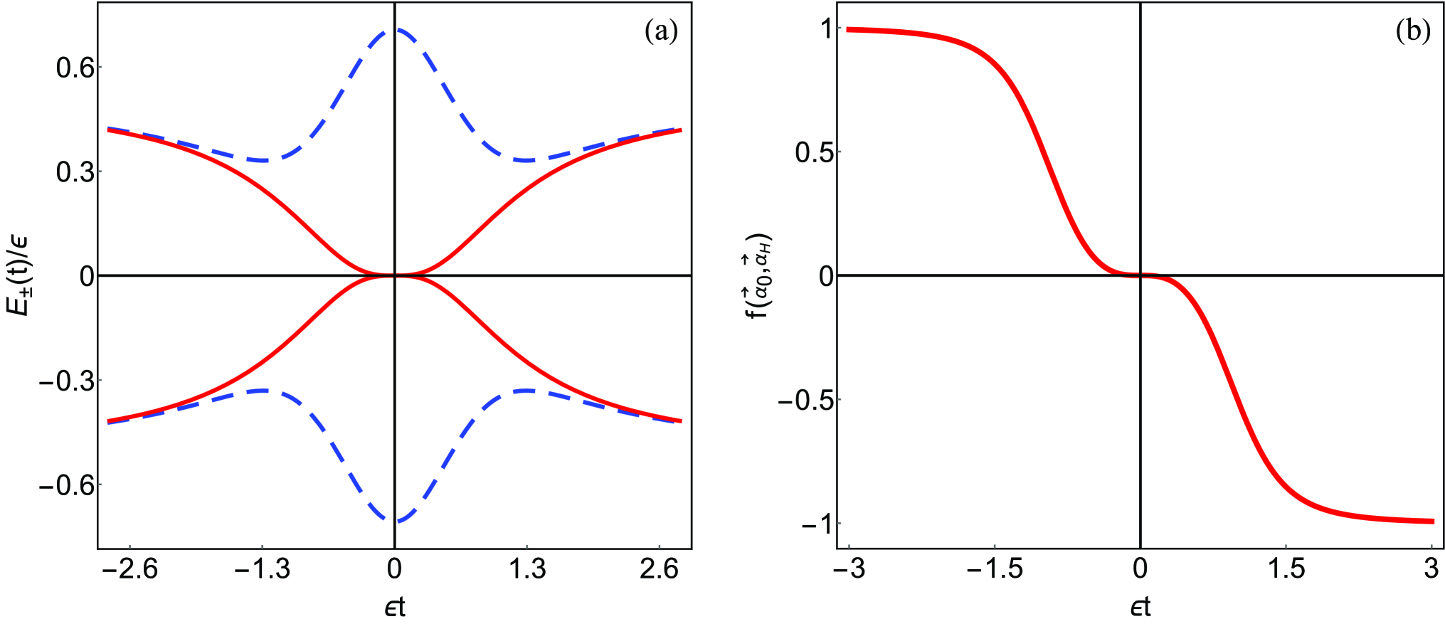
Figure 1: The NLC phenomenon of the model (2) with $j=\frac{1}{2}$. (a) The two nonadiabatic energy levels $E_{\pm}(t)$ over $\epsilon$ which intersect at $t_{c}=0$. The dashed lines stand for the instantaneous adiabatic energies $E_{\pm}^{ad}(t)$ over $\epsilon$ which exhibit the avoided level crossing twice. (b) The inner product $f(\vec{\alpha}_{0},\vec{\alpha}_{h})$ changes from $+1$ to $-1$ and vanishes at $t_{c}=0$.

With the above analytical solution, we are able to describe the anomaly of the dynamical evolution of the model. It is seen that as $t$ goes from $-\infty$ to $+\infty$, the invariant $I(t)$ will go from $+J_{z}$ to $-J_{z}$. Indeed, the two representative vectors $\vec{\alpha}_{h}(t)$ and $\vec{\alpha}_{0}(t)$, accounting respectively for the orientation of $H(t)$ and $I(t)$ in the parametric space, will evolve from the parallel state with $\theta_{h}=\theta_{0}=0$ to the antiparallel state with $\theta_{h}=0$ and $\theta_{0}=\pi$. Therefore, the nonadiabatic basis state $|\psi_{m}(t)\rangle$ exhibits the opposite behavior from the adiabatic state $|\psi_{m}^{ad}(t)\rangle$ as it leads to a complete population inversion $|m\rangle\leftrightarrow|-m\rangle$ during the evolution. Furthermore, the peculiarity of the dynamical behavior can also be recognized from the different crossing phenomena of the corresponding adiabatic and nonadiabatic energy levels. As the adiabatic levels exhibit only avoided crossings, the nonadiabatic levels of the model, formulated as

$$E_{m}(t) \equiv \langle\psi_{m}(t)|H(t)|\psi_{m}(t)\rangle$$ (7)

$$= -\frac{m\epsilon^{4}t^{3}}{(1+\epsilon^{2}t^{2})^{3/2}},$$

exhibit a real crossing at $t_{c}=0$. For the two-level case with the azimuthal quantum number $j=\frac{1}{2}$, these level crossing phenomena are illustrated in Fig. 1(a).

III General description of the protocol

III.1 Condition associated with the nonadiabatic level crossing

To reveal the connection between the above described anomalous dynamical evolution and the NLC phenomenon, it is worthy to note that at the crossing point $t_{c}=0$ the orientation of $\vec{\alpha}_{h}$ is vertical to $\vec{\alpha}_{0}$ as $\vec{\alpha}_{h}$ is fixed in the $x$-$z$ plane and $\vec{\alpha}_{0}(t_{c})=(0,-1,0)$ is exactly along the $y$ axis. In fact, this is not accidental in view that the nonadiabatic level $E_{m}(t)$ can be expressed as

$$E_{m}(t) = \langle\phi_{m}(t)|H(t)|\phi_{m}(t)\rangle$$ (8)

$$= \langle m|e^{-i\theta_{0}J_{y}}e^{-i(\pi-\varphi_{0})J_{z}}H(t)e^{i(\pi-\varphi_{0})J_{z}}e^{i\theta_{0}J_{y}}|m\rangle$$

$$= m\vec{\Omega}(t)\cdot\vec{\alpha}_{0}(t).$$

That is to say, there exists a general correspondence between the orthogonal relation $\vec{\alpha}_{0}\cdot\vec{\alpha}_{h}=0$ and the NLC with all $E_{m}=0$. The evolution of the inner product $f(\vec{\alpha}_{0},\vec{\alpha}_{h})\equiv\vec{\alpha}_{0}(t)\cdot\vec{\alpha}_{h}(t)$ of the model (2) is illustrated in Fig. 1(b). Mathematically, the orthogonality here can also be understood as that the two operators, $I(t)$ and $H(t)$, have vanishing Frobenius inner product froben : $\mathrm{tr}[I(t_{c})H(t_{c})]=0$. As a consequence, the occurring of the NLC can be identified as a necessity condition of the anomalous dynamical evolution: as the two vectors $\vec{\alpha}_{0}(t)$ and $\vec{\alpha}_{h}(t)$ change continuously from a parallel state to an anti-parallel state in the parametric space, it is unavoidable that they should go through a perpendicular position during the evolution.

III.2 The reverse-engineering scheme

In the light of the above result, we now address the question how to achieve such kind of driven quantum systems with the similar anomalous dynamical behavior. To this end, let us consider the dynamics generated by the driven model of Eq. (2) with general field pulses $\Omega_{x}(t)$ and $\Omega_{z}(t)$. We suppose that the system possesses a dynamical invariant $I(t)\equiv\vec{\alpha}(t)\cdot\vec{J}$ with its components $\alpha_{i}(t)$ fulfilling

$$\dot{\alpha}_{x}(t) = -\Omega_{z}(t)\alpha_{y}(t),$$ (9)

$$\dot{\alpha}_{y}(t) = \Omega_{z}(t)\alpha_{x}(t)-\Omega_{x}(t)\alpha_{z}(t),$$ (10)

$$\dot{\alpha}_{z}(t) = \Omega_{x}(t)\alpha_{y}(t).$$ (11)

Since the eigenvalues of $I(t)$ are independent of time, we can set $|\vec{\alpha}(t)|=1$ and express it as $\vec{\alpha}(t)=(\sin\theta\cos\varphi,\sin\theta\sin\varphi,\cos\theta)$. We then regard Eqs. (9)-(11) as algebraic equations of $\Omega_{x,z}(t)$. Explicitly, Eq. (11) indicates

$$\Omega_{x}(t)=-\frac{\dot{\theta}(t)}{\sin\varphi(t)},$$ (12)

and Eq. (9) [or Eq. (10) equivalently] indicates

$$\Omega_{z}(t) = \dot{\varphi}(t)+\Omega_{x}(t)\cot\theta(t)\cos\varphi(t)$$ (13)

$$= \dot{\varphi}(t)-\dot{\theta}(t)\cot\theta(t)\cot\varphi(t).$$

That is to say, for any given $I(t)$ with specified $\theta(t)$ and $\varphi(t)$, one can construct the field components $\Omega_{x,z}(t)$ in virtue of Eqs. (12) and (13). Note that similar reverse-engineering schemes have ever been proposed, e.g., in Refs. berry and inverLR . In comparison, there is no redundant parameter in the present scheme and the driving field of the target Hamiltonian here is uniquely determined. On other words, it indicates that the driving protocol with two field components is sufficient to generate any desired SU(2) rotation to the wavefunction.

If we set $\theta(t)=\theta_{0}(t)$ and $\varphi(t)=\varphi_{0}(t)$ specified in Eq. (5) and substitute them into Eqs. (12) and (13), one promptly obtains the previous model of Eq. (2). To illustrate the selection of $\theta(t)$ and $\varphi(t)$ and the resulting anomalous dynamical behavior, one is led to notice that as $t\rightarrow\pm\infty$, there is $\dot{\varphi}_{0}(t)\rightarrow 0$ and $\Omega_{z}$ is then dominated by the term $\Omega_{x}\cot\theta_{0}\cos\varphi_{0}$ [cf. Eq. (13)]. So the relation between the two angles $\theta_{0}$ and $\theta_{h}$ at $t\rightarrow\pm\infty$ is characterized by

$$\cot\theta_{h}=\cos\varphi_{0}\cot\theta_{0}.$$ (14)

The change of the relative orientation of $\vec{\alpha}_{h}(t)$ and $\vec{\alpha}_{0}(t)$, i.e., from the parallel state to the antiparallel state, is then well understood because $\cos\varphi_{0}$, according to Eq. (5), alters its sign (from $+1$ to $-1$) during the evolution. This illuminates a way to contrive similar driving protocols with the anomalous dynamical behavior.

III.3 Further examples of the driving protocol

For the second example let us consider a single-axis driven model described by

$$H(t)=\epsilon J_{x}+\Omega_{z}(t)J_{z},$$ (15)

in which $\Omega_{x}=\epsilon$ is time independent and the driving component $\Omega_{z}(t)$ is given by

$$\Omega_{z}(t)=\frac{5\epsilon e^{2\epsilon t}-\epsilon e^{6\epsilon t}}{1+e^{4\epsilon t}}.$$ (16)

This model can be constructed from Eqs. (12) and (13) by setting the two angles as

$$\theta(t)=\frac{\pi}{2}-\arctan e^{2\epsilon t},~{}~{}\varphi(t)=2\arctan e^{2\epsilon t}.$$ (17)

As $t$ goes from $-\infty$ to $+\infty$, these angles will go from $(\theta,\varphi)=(\frac{\pi}{2},0)$ to $(\theta,\varphi)=(0,\pi)$. Differing from the former model, the representative vectors $\vec{\alpha}_{h}(t)$ and $\vec{\alpha}(t)$ of the Hamiltonian and of the dynamical invariant here, are along the $+x$ axis initially at $t\rightarrow-\infty$. They arrive eventually at an anti-parallel state, $\vec{\alpha}_{h}(t)\rightarrow-z$ and $\vec{\alpha}(t)\rightarrow+z$ as $t\rightarrow+\infty$. The anomalous dynamical behavior can be specified explicitly by the evolution of the wavefunction. The instantaneous adiabatic states, say, for the two-level case with azimuthal quantum number $j=\frac{1}{2}$, will evolve as

$$|\psi_{\pm}^{ad}(-\infty)\rangle=\frac{\sqrt{2}}{2}(|+\rangle\pm|-\rangle)\stackrel{{\scriptstyle t\rightarrow+\infty}}{{\longrightarrow}}|\mp\rangle,$$ (18)

in which we have used the notation “$\pm$” for “$\pm\frac{1}{2}$”. In comparison, the eigenstate of $I(t)$, accounting for the the nonadiabatic evolution of the system, will evolve as

$$|\phi_{\pm}(-\infty)\rangle=\frac{\sqrt{2}}{2}(|+\rangle\pm|-\rangle)\stackrel{{\scriptstyle t\rightarrow+\infty}}{{\longrightarrow}}|\pm\rangle.$$ (19)

That is, the nonadiabaticity of the evolution induces a complete exchange between the two adiabatic basis states as $t\rightarrow+\infty$.

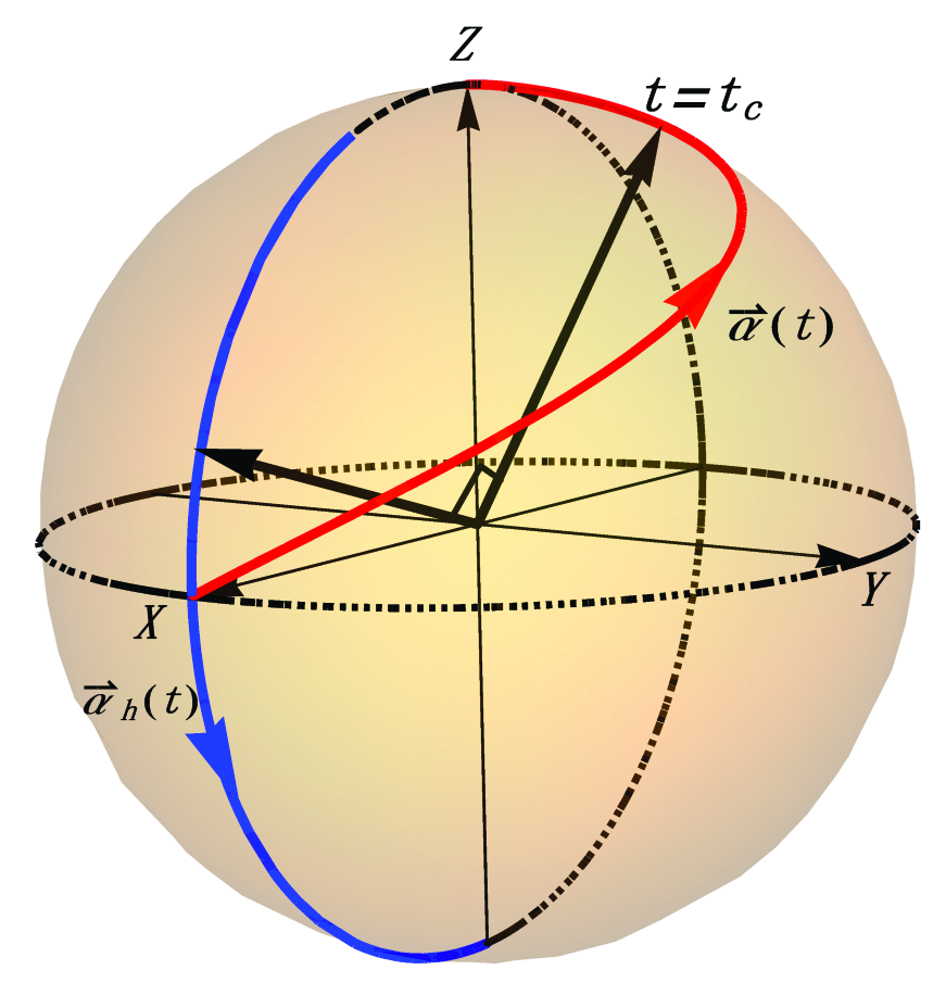
Figure 2: Illustration of the evolving trajectories of the two vectors $\vec{\alpha}_{h}(t)$ and $\vec{\alpha}(t)$ in the parametric space of the model specified by Eq. (15). At $t=t_{c}$ the two vectors are shown to be vertical to each other [cf. Eqs. (21) and (22)].

On the other hand, the nonadiabatic energy level of the system is worked out to be

$$E_{m}(t)=m\epsilon\left[\frac{4e^{4\epsilon t}}{(1+e^{4\epsilon t})^{3/2}}-\frac{e^{4\epsilon t}-1}{(1+e^{4\epsilon t})^{1/2}}\right].$$ (20)

It is straightforward to verify that as $\epsilon t_{c}=\frac{1}{4}\ln(2+\sqrt{5})$ there is $E_{m}(t_{c})=0$, that is, all the nonadiabatic energy levels should intersect at the particular point $t=t_{c}$. Specifically, at the point of $\epsilon t_{c}=\frac{1}{4}\ln(2+\sqrt{5})$, there are

$$\vec{\alpha}(t_{c})=(\frac{\sqrt{10}-3\sqrt{2}}{4},\frac{\sqrt{2\sqrt{5}-4}}{2},\frac{\sqrt{\sqrt{5}+1}}{2}),$$ (21)

and

$$\vec{\Omega}(t_{c})/\epsilon=(1,0,\frac{\sqrt{10\sqrt{5}-22}}{2}).$$ (22)

So the orthogonality of these two vectors at the crossing point $t=t_{c}$ can be verified straightforwardly. In Fig. 2 we plot the schematic of the evolving trajectories of $\vec{\alpha}(t)$ and $\vec{\alpha}_{h}(t)$ for the model in the parametric space.

To obtain the third protocol, we set $\theta(t)$ and $\varphi(t)$ as

$$\theta(t)=\arccos[\tanh(2\epsilon t)],~{}~{}\varphi(t)=\frac{\pi}{2}-\arctan[\tanh(\epsilon t)],$$ (23)

via which the driving field components are achieved as

$$\Omega_{x}(t)=2\epsilon\mbox{sech}(\epsilon t)\mbox{sech}^{\frac{1}{2}}(2\epsilon t),~{}~{}\Omega_{z}(t)=\epsilon[3\mbox{sech}(2\epsilon t)-2].$$ (24)

The curves of the field pulses $\Omega_{x}(t)$ and $\Omega_{z}(t)$ are plotted in Fig. 3(a). According to Eq. (23), $\cos\varphi$ will evolve from $-\frac{\sqrt{2}}{2}$ to $\frac{\sqrt{2}}{2}$ as the time goes from $-\infty$ to $+\infty$. So the ratio $\cot\theta_{h}/\cot\theta$ should alter its sign at $t\rightarrow\pm\infty$ according to Eq. (14). Specifically, the orientation of $\vec{\alpha}(t)$ will go from $-z$ to $+z$, so the complete population transfer $|m\rangle\leftrightarrow|-m\rangle$ can be realized through the nonadiabtic evolution. On the other hand, as $\vec{\alpha}_{h}(t)$ tends to the $-z$ axis as $t\rightarrow\pm\infty$, the adiabatic state will return to its initial state. At $t=0$, there are $\theta(0)=\varphi(0)=\frac{\pi}{2}$, which indicates that $\vec{\alpha}(0)$ is along the $y$ axis, hence is vertical with $\vec{\alpha}_{h}(t)$ at that time instant. In Fig. 3(b) we depict the corresponding NLC for the model with $j=\frac{1}{2}$.

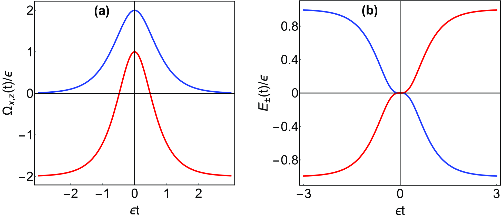
Figure 3: The field pulses $\Omega_{x,z}(t)$ and the nonadiabatic levels of the model specified by Eq. (24). (a) The field component $\Omega_{x}(t)$ (the upper curve) vanishes as $t\rightarrow\pm\infty$ while the component $\Omega_{z}(t)=-2\epsilon$ as $t\rightarrow\pm\infty$. (b) The nonadiabatic energy levels $E_{\pm}(t)$ of the model which exhibit the real NLC at $t_{c}=0$.

IV Discussion and conclusion

The anomalous dynamical evolution described above represents the extreme behavior associated with the nonadiabatic driving. It is worthy to mention that such an extreme manifestation of the nonadiabtic effect could also be found in the standard LZ model. According to the LZ formula, the nonadiabatic transition between the two adiabatic states over the whole evolution is specified by $P=e^{-\frac{\pi\Delta^{2}}{2\nu}}$ in which $\Delta$ describes the constant coupling between the two bare states and $\nu$ stands for the scanning rate of the linearly driving field. If the scanning rate satisfies $\nu/\Delta^{2}\rightarrow+\infty$, the nonadiabtic evolution will lead to completely opposite behavior with that of the instantaneous adiabtic state. In comparison, the driving fields in all our proposed protocols have finite scanning rate hence are more realistic physically.

The driven model with the anomalous dynamical evolution offers an alternative scenario for the state transfer that is distinctly different from the existing schemes, e.g., the transitionless quantum driving berry , the so-called shortcut-to-adiabaticity protocol counter ; short and their recent development short2 . Given a general time-dependent Hamiltonian $H(t)$, the transitionless algorithm cancels out the nonadiabatic effect by introducing an auxiliary counter-diabatic field and ensures that the dynamical evolution of the system follows a normal trajectory, i.e., remains in the instantaneous eigenstate of $H(t)$. In this sense, the strategies of the anomalous dynamical evolution and of those existing protocols are complementary and may have different applications to the design of quantum state control in experimental systems.

To summarize, we have investigated the anomalous dynamical evolution for the time-dependent quantum systems by virtue of a reverse-engineering method. Our study demonstrates that the occurring of the anomaly, i.e., the evolution of the nonadiabatic states exhibits opposite behavior with that of the adiabatic ones, is always concomitant with the NLC in these nonadiabtically driven systems. In particular, we have proposed three cases of such kind of driving protocols. In all these protocols the relative orientation of the representative vectors of the adiabatic and nonadiabatic bases undergoes a change from the parallel state to the antiparallel state, and the nonadiabatic levels of each system exhibit the anticipated crossing phenomenon.

References

- (1) L.D. Landau, Phys. Z. Sowjetunion 2, 46 (1932).
- (2) C. Zener, Proc. R. Soc. A 137, 696 (1932).
- (3) C.F. Bharucha, K.W. Madison, P.R. Morrow, S.R. Wilkinson, B. Sundaram, M.G. Raizen, Phys. Rev. A 55, R857 (1997).
- (4) K. Saito, M. Wubs, S. Kohler, P. Hänggi, Y. Kayanuma, Europhys. Lett. 76, 22 (2006).
- (5) A. Zenesini, H. Lignier, G. Tayebirad, J. Radogostowicz, D. Ciampini, R. Mannella, S. Wimberger, O. Morsch, E. Arimondo, Phys. Rev. Lett. 103, 090403 (2009).
- (6) R. Khomeriki, Phys. Rev. A 82, 013839 (2010).
- (7) N. Malossi, M.G. Bason, M. Viteau, E. Arimondo, R. Mannella, O. Morsch, D. Ciampini, Phys. Rev. A 87, 012116 (2013).
- (8) A.M. Kuztetsov, Charge Transfer in Physics, Chemistry, and Biology, Gordon and Breach: Reading, 1995.
- (9) C. Zhu, S.H. Lin, J. Chem. Phys. 107, 2859 (1997).
- (10) A. Nitzan, Chemical Dynamics in Condensed Phases, Oxford University Press: Oxford, 2006.
- (11) H. Nakamura, Nonadiabatic transitions: Concepts, Basic Theories and Applications, World Scientific, 2012.
- (12) L.F. Wei, J.R. Johansson, L.X. Cen, S. Ashhab, F. Nori, Phys. Rev. Lett. 100, 113601 (2008).
- (13) J.Q. You, F. Nori, Nature 474, 589 (2011).
- (14) G. Cao, H.O. Li, T. Tu, L. Wang, C. Zhou, M. Xiao, G.C. Guo, H.W. Jiang, G.P. Guo, Nat. Commun. 4, 1401 (2012).
- (15) C.M. Quintana, K.D. Petersson, L.W. McFaul, S.J. Srinivasan, A.A. Houck, J.R. Petta, Phys. Rev. Lett. 110, 173603 (2013).
- (16) M.B. Kenmoe, L.C. Fai, Phys. Rev. B 94, 125101 (2016).
- (17) G. Yang, W. Li, L.X. Cen, Chin. Phys. Lett. 35, 013201 (2018).
- (18) W. Li, L.X. Cen, Ann. Phys. 389, 1 (2018).
- (19) J.R. Rubbmark, M.M. Kash, M.G. Littman, D. Kleppner, Phys. Rev. A 23, 3107 (1981).
- (20) G. Sun, X. Wen, Y. Wang, S. Cong, J. Chen, L. Kang, W. Xu, Y. Yu, S. Han, P. Wu, Appl. Phys. Lett. 94, 102502 (2009).
- (21) T. Wang, Z. Zhang, L. Xiang, Z. Jia, P. Duan, W. Cai, Z. Gong, Z. Zong, M. Wu, J. Wu, New J. Phy. 20, 065003 (2018).
- (22) J. Zhang, J.H. Shim, I. Niemeyer, T. Taniguchi, T. Teraji, H. Abe, S. Onoda, T. Yamamoto, T. Ohshima, J. Isoya, D. Suter, Phys. Rev. Lett. 110, 240501 (2013).
- (23) B.D. Militello, N.V. Vitanov, Phys. Rev. A. 91, 053402 (2015).
- (24) H.R. Lewis, Phys. Rev. Lett. 18, 510 (1967).
- (25) H.R. Lewis, W.B. Riesenfeld, J. Math. Phys. 10, 1458 (1969).
- (26) C.D. Meyer, Matrix Analysis and Applied Linear Algebra, SIAM, 2000.
- (27) M.V. Berry, J. Phys. A 42, 365303 (2009).
- (28) X. Chen, E. Torrontegui, J.G. Muga, Phys. Rev. A 83, 062116 (2011).
- (29) M. Demirplak, S.A. Rice, J. Phys. Chem. A 107, 9937 (2003).
- (30) X. Chen, T. Lizuain, A. Ruschhaupt, D. Guéry-Odelin, J.G. Muga, Phys. Rev. Lett. 105, 123003 (2010).
- (31) F. Petiziol, B. Dive, F. Mintert, S. Wimberger, Phys. Rev. A 98, 043436 (2018).