Explicit construction of nonadiabatic passages for stimulated Raman transitions

Abstract

We propose a scheme which can produce desired nonadiabatic passages for the stimulated Raman transition in three-level systems. The state transfer in the protocol is realized by following the evolution of the dynamical basis itself and no additional coupling field is required. We also investigate the interplay between the present nonadiabatic protocol and the shortcut to adiabaticity. By incorporating the latter technology, we show that alternative passages with less occupancy of the intermediate level could be designed.

I Introduction

Stimulated Raman adiabatic passage (STIRAP) is an efficient technique for robust coherent population transfer in atomic and molecular systems, which has been extensively investigated over the past decades raman0 ; raman1 ; raman2 ; raman3n ; raman3 ; raman4 . It can induce transitions between two levels that has the same parity, for which the direct coupling via electric dipole radiation is forbidden. Specifically, the STIRAP applies two laser pulses, the pump and Stokes, to induce the coupling between each of the two levels and a common intermediate level under the condition of the two-photon resonance. The desired population transfer is realized through the adiabatic evolution of the dark state, which conventionally assumes a superposition form of the initial and the final target states.

Based on the transitionless tracking algorithm counter ; counter2 ; berry , the shortcut to adiabaticity shortcut1 ; shortcut2 ; shortcut3 ; shortcut33 ; shortcut4 ; shortcut5 ; shortcut6 has been exploited to speed up the evolution of the STIRAP. In the initial proposals shortcut2 ; shortcut3 of the stimulated Raman shortcut-to-adiabatic passage (STIRSAP), the application of a compensating microwave field which couples the initial and target states is required to counteract the detrimental nonadiabatic effect. This additional microwave field indicates a critical disadvantage, especially concerning that the direct coupling might be unfeasible in practical atomic levels with forbidden transition. In the subsequent proposals shortcut4 ; shortcut5 , it is displayed that one can mimic the desired population transfer of the STIRSAP protocol through modifying the pump and Stokes pulses, which removes the coupling term associated with the microwave field so as to avoid the former drawback. Strictly, in this modified STIRSAP scheme the evolution of the wavefunction (so called as the “dressed state” in Ref. shortcut4 ) differs from that in the former one by a rotating transformation $V(t)$. The validity of the scheme then relies on the boundary condition of $V(t)$, that is, $V(t)$ should be a null operation at the initial (ending) time instant.

Successful design of the laser pulses for the STIRSAP is critically constrained by the above boundary condition of the dressed-state transformation. For example, this condition is not satisfied when the pump and the Stokes fields assume the commonly used Gaussian pulses shortcut4 ; shortcut5 . Note that the rotating angle of $V(t)$ is correlated to the aforementioned microwave field that should have been applied in the initial STIRSAP protocol. The specified boundary condition of $V(t)$ can be fulfilled only when the strength of this additional interaction, or equally speaking, the nonadiabatic effect induced by the initial pump and Stokes fields, should be negligible on the boundary. This actually requires that the driving protocol should satisfy the adiabatic condition at that time instant. At this stage, a promising design may rest on (but not limited to) the prerequisite that the system should possess discrete energy levels at the initial (ending) instant of the driving pulses.

On the other hand, valuable results have been obtained recently in understanding the nonadiabatic dynamics generated by some particular types of quantum driven models model1 ; model2 ; model3 ; model4 . It is shown that the nonadiabatic effect in some of the cases can play a positive role for the population transfer. For example, in the tangent-pulse-driven model with the matching frequency and amplitude, the nonadiabatic effect not only will not lead to unwanted transitions but also can suppress the error caused by the truncation of the field pulse model1 . This feature of the nonadiabatic driving has also been found in a modified Landau-Zener model model2 and a special Allen-Eberly model model3 . Motivated by these results, it is natural to ask whether there exists such kind of nonadiabatic passages that can be exploited directly to realize the stimulated Raman process.

In this paper we report the finding of a specific driving scheme via which the nonadiabatic passages of the stimulated Raman transition can be explicitly constructed. The scheme applies to the $\Lambda$-type three-level system with the one-photon resonance in which the Stokes laser pulse can be of arbitrary analytical form but the pump pulse should be matching with the Stokes one. Several driving protocols generated by the scheme are illustrated and there various features for the population transfer are characterized. Moreover, we explore the interplay of the present scheme with the STIRSAP and show how to reconstruct the nonadiabatic passages within the framework of the shortcut to adiabaticity. Incorporation with the latter technology enables us to design alternative nonadiabatic passages with less occupancy of the intermediate level.

II Stimulated Raman nonadiabatic passages with one-photon resonance

II.1 Description of the driving scheme

Consider a three-level system with the $\Lambda$ configuration shown in Fig. 1. The states $|1\rangle$ and $|3\rangle$ are ground or metastable levels, which are coupled to the excited level $|2\rangle$ via the laser pulses, the pump pulse and the Stokes pulse, respectively. The Hamiltonian of the system under the rotating wave approximation can be written as $H_{\rm{tot}}(t)=H_{\rm{free}}+H_{\rm{int}}(t)$ with the free Hamiltonian $H_{\rm{free}}=\sum_{i=1}^{3}E_{i}\sigma_{ii}$ and the interaction term

$$H_{\rm{int}}(t) = \Omega_{p}(t)(\sigma_{12}e^{i\omega_{p}t}+\sigma_{21}e^{-i\omega_{p}t})$$ (1)

$$+\Omega_{s}(t)(\sigma_{23}e^{-i\omega_{s}t}+\sigma_{32}e^{i\omega_{s}t}),$$

in which $\sigma_{ij}=|i\rangle\langle j|$ $(i,j=1,2,3)$ and $\Omega_{p,s}(t)$ describe the Rabi frequencies of the pump and Stokes pulses, respectively. Under the condition of the one-photon resonance $\omega_{p}=E_{2}-E_{1}$ and $\omega_{s}=E_{2}-E_{3}$, one obtains the Hamiltonian in the interaction picture

$$H(t)=\Omega_{p}(t)(\sigma_{12}+\sigma_{21})+\Omega_{s}(t)(\sigma_{23}+\sigma_{32}).$$ (2)

To implement fast population transfer from the state $|1\rangle$ to $|3\rangle$, we propose a nonadiabatic protocol in which the laser pulses satisfy

$$\Omega_{p}(t)=\frac{1}{2}\Omega_{s}(t)\sec[\frac{1}{2}\int_{t_{0}}^{t}\Omega_{s}(\tau)d\tau]$$ (3)

with the envelope of the Stokes laser $\Omega_{s}(t)$ being an arbitrary analytical function over $t\in(t_{0},t_{f})$. As is shown in the below, when the integral of the intercepted pulse $\int_{t_{0}}^{t}\Omega_{s}(\tau)d\tau\equiv 2\vartheta(t)$ goes from $0$ to $\pi$, complete population transfer $|1\rangle\rightarrow|3\rangle$ can be realized by the protocol in a nonadiabatic manner.

Figure 1: Schematic of the level structure of the three-level system, where $\Omega_{p}$ and $\Omega_{s}$ denote the Rabi frequencies of the pump and Stokes laser pulses, respectively.

To resolve the dynamics of the above stimulated Raman process, we note that the described model possesses a dynamical invariant lewis1 ; lewis2

$$I(t) = \sin^{2}\vartheta(t)(\sigma_{12}+\sigma_{21})+\cos\vartheta(t)(\sigma_{23}+\sigma_{32})$$ (4)

$$-i\sin\vartheta(t)\cos\vartheta(t)(\sigma_{13}-\sigma_{31}),$$

which satisfies

$$\partial_{t}I(t)=-i[H(t),I(t)].$$ (5)

It is recognized that the three operators $K_{x}\equiv\sigma_{12}+\sigma_{21}$, $K_{y}\equiv i(\sigma_{13}-\sigma_{31})$ and $K_{z}\equiv\sigma_{23}+\sigma_{32}$ satisfy the commutation relation $[K_{\alpha},K_{\beta}]=i\epsilon_{\alpha\beta\gamma}K_{\gamma}$. By recording $I(t)=\vec{\chi}(t)\cdot\vec{K}$, Eq. (5) is readily verified through the following equations of the components

$$\dot{\chi}_{1}(t) = -\Omega_{s}(t)\chi_{2}(t),$$ (6)

$$\dot{\chi}_{2}(t) = \Omega_{s}(t)\chi_{1}(t)-\Omega_{p}(t)\chi_{3}(t),$$ (7)

$$\dot{\chi}_{3}(t) = \Omega_{p}(t)\chi_{2}(t).$$ (8)

The eigenvalues of $I(t)$ are given by $\lambda_{0}=0$ and $\lambda_{\pm}=\pm 1$, and the eigenstate $|e_{0}(t)\rangle$ associated with the zero eigenvalue $\lambda_{0}$ is obtained as

$$|e_{0}(t)\rangle=\cos\vartheta|1\rangle-i\sin\vartheta\cos\vartheta|2\rangle-\sin^{2}\vartheta|3\rangle.$$ (9)

It is seen that the initial state $|1\rangle$ correlates exclusively with the basis state $|e_{0}(t)\rangle$, so the wavefunction will evolve along this “dressed state” for the time being. Since the corresponding eigenvalue $\lambda_{0}=0$, the Lewis-Riesenfeld phase lewis1 ; lewis2 accumulated during the evolution is zero for $|e_{0}(t)\rangle$. As $\vartheta(t_{f})\rightarrow\frac{\pi}{2}$, the state transfer $|1\rangle\rightarrow|3\rangle$ is achieved up to a minus sign.

A particular feature one can recognize from the above stimulated Raman protocol is that at the initial $t=t_{0}$ there is $\Omega_{p}(t_{0})=\frac{1}{2}\Omega_{s}(t_{0})$. This is distinctly different from the delayed pulse sequence of the adiabatic passage, which indicates that the nonadiabatic effect plays a decisive role in the present protocol. It also reveals that the Hamiltonian and the dynamical invariant are not commutative at $t=t_{0}$: $[H(t_{0}),I(t_{0})]\neq 0$, which does not accord with the condition assumed in Ref. shortcut2 . Secondly, as $t\rightarrow t_{f}$ the asymptotic population on the target state $|3\rangle$ is specified by $P(t)=\sin^{4}\vartheta(t)$. It indicates that the protocol is less sensitive to the cutoff error of the field pulses than the adiabatic protocol. In detail, suppose that the field pulses are truncated at $t=t_{fc}$ with the Rabi frequencies $\Omega_{p}(t_{fc})$ and $\Omega_{s}(t_{fc})$. Denote by $\delta\equiv\arctan\frac{\Omega_{s}(t_{fc})}{\Omega_{p}(t_{fc})}$ the deviation of the pulses. The population on $|3\rangle$ at $t=t_{fc}$ is then given by

$$P(t_{fc})=\sin^{4}\vartheta(t_{fc})=(1-\frac{1}{4}\tan^{2}\delta)^{2}.$$ (10)

As $\delta$ is much less that $1$, it is not difficult to verify that there is always $P(t_{fc})\geq\cos^{2}\delta$. That is to say, comparing with the conventional STIRAP, the nonadiabatic effect in the present protocol will reduce the loss of fidelity caused by the truncation.

II.2 Typical nonadiabatic passages

The above scheme offers an explicit way to construct stimulated Raman nonadiabatic passages via which the population transfer $|1\rangle\rightarrow|3\rangle$ can be realized. We present some typical examples in the below.

Example 1. The Rabi frequency of the Stokes laser is set to be a constant. According to Eq. (3), there are

$$\bigg{\{}\begin{array}[]{l}\Omega_{p}(t)=\frac{\nu}{2}\sec\frac{\nu t}{2},\\ \Omega_{s}(t)=\nu,\end{array}$$ (11)

in which the time $t$ goes from $t=0$ to $t\rightarrow\frac{\pi}{\nu}$. The dynamical invariant and the zero-eigenvalue dress state are specified by

$$I(t) = \sin^{2}\frac{\nu t}{2}(\sigma_{12}+\sigma_{21})+\cos\frac{\nu t}{2}(\sigma_{23}+\sigma_{32})$$ (12)

$$-\frac{i}{2}\sin\nu t(\sigma_{13}-\sigma_{31})$$

and

$$|e_{0}(t)\rangle=\cos\frac{\nu t}{2}|1\rangle-\frac{i}{2}\sin(\nu t)|2\rangle-\sin^{2}\frac{\nu t}{2}|3\rangle,$$ (13)

respectively. In this proposal the pump laser assumes a chirped pulse and the duration of the pulse $\nu t_{f}\approx\pi$ is much shorter than that of the usual adiabatic protocol.

Example 2. The passage is described by

$$\bigg{\{}\begin{array}[]{l}\Omega_{p}(t)=\nu,\\ \Omega_{s}(t)=2\nu\mathrm{sech}(\nu t),\end{array}$$ (14)

in which $\Omega_{p}(t)$ of the pump laser is a constant. The two Rabi frequencies above are verified to satisfy Eq. (3) in view that the half of the integration of $\Omega_{s}(t)$ gives rise to $\vartheta(t)=\arctan[\sinh(\nu t)]$. The eigenstate $|e_{0}(t)\rangle$ of the dynamical invariant is obtained as

$$|e_{0}(t)\rangle=\mathrm{sech}(\nu t)|1\rangle-i\tanh(\nu t)\mathrm{sech}(\nu t)|2\rangle-\tanh^{2}(\nu t)|3\rangle.$$ (15)

The field pulses in this protocol are defined in an infinite time domain and the truncation is inevitable. We define an effective pulse duration $t\in(t_{0},t_{fc})$ in which $t_{fc}$ is defined such that the population on $|3\rangle$ reaches $P(t_{fc})\approx 0.9999$. For the current example there is $\nu t_{fc}\approx 1.8\pi$.

In principle, unlimited amount of the nonadiabatic passages could be constructed by the scheme. Besides the above two, some other examples are displayed in Table I, including the field pulses, evolution of the population, and their effective pulse duration.

Table 1: Various nonadiabatic passages and their pulse durations generated by the scheme.

	Stokes Pulse	Pump Pulse	Target State Pop.	$\nu t_{fc}$	$\Omega_{s0}(t)$	$\Omega_{p0}(t)$
$(a)$	$\Omega_{s}=\nu$	$\Omega_{p}=\frac{\nu}{2}\sec\frac{\nu t}{2}$	$\sin^{4}\frac{\nu t}{2}$	$\approx\pi$	$\frac{\nu}{2}$	$\frac{\nu}{2}\tan(\frac{\nu t}{2})$
$(b)$	$\Omega_{s}=2\nu\mathrm{sech}(\nu t)$	$\Omega_{p}=\nu$	$\tanh^{4}(\nu t)$	$\approx 1.80\pi$	$\nu\mathrm{sech}(\nu t)$	$\nu\tanh(\nu t)$
$(c)$	$\Omega_{s}=\frac{2\nu}{\sqrt{1-\nu^{2}t^{2}}}$	$\Omega_{p}=\frac{\nu}{1-\nu^{2}t^{2}}$	$\nu^{4}t^{4}$	$\approx 1$	$\frac{\nu}{\sqrt{1-\nu^{2}t^{2}}}$	$\frac{\nu^{2}t}{1-\nu^{2}t^{2}}$
$(d)$	$\Omega_{s}=\nu^{2}t$	$\Omega_{p}=\frac{\nu^{2}t}{2}\sec\frac{\nu^{2}t^{2}}{4}$	$\sin^{4}\frac{\nu^{2}t^{2}}{4}$	$\approx 0.80\pi$	$\frac{\nu^{2}t}{2}$	$\frac{\nu^{2}t}{2}\tan(\frac{\nu^{2}t^{2}}{4})$
$(e)$	$\Omega_{s}=4\nu^{2}t\mathrm{sech}(\nu^{2}t^{2})$	$\Omega_{p}=2\nu^{2}t$	$\tanh^{4}(\nu^{2}t^{2})$	$\approx 0.76\pi$	$2\nu^{2}t\mathrm{sech}(\nu^{2}t^{2})$	$2\nu^{2}t\tanh(\nu^{2}t^{2})$
$(f)$	$\Omega_{s}=2\nu e^{\nu t}$	$\Omega_{p}=\nu e^{\nu t}\sec(e^{\nu t}-1)$	$\sin^{4}(e^{\nu t}-1)$	$\approx 0.30\pi$	$\nu e^{\nu t}$	$\nu e^{\nu t}\tan(e^{\nu t}-1)$

III Interplay with the shortcut to adiabaticity

III.1 Stimulated Raman shortcut-to-adiabatic passage and the dressed-state transformation

To be specific, let us review the STIRSAP protocol with the one-photon resonance of which the initial Hamiltonian in the interaction picture reads

$$H_{0}(t)=\Omega_{p0}(t)(\sigma_{12}+\sigma_{21})+\Omega_{s0}(t)(\sigma_{23}+\sigma_{32}).$$ (16)

In general, the sequence of the delayed pulse interactions of the pump and the Stokes lasers are implemented in the counterintuitive order so that the Rabi frequencies satisfy $\Omega_{s0}(t_{0})\gg\Omega_{p0}(t_{0})$ and $\Omega_{s0}(t_{f})\ll\Omega_{p0}(t_{f})$ at the initial and the ending time $t_{0,f}$, respectively. For the adiabatic evolution the state transfer $|1\rangle\rightarrow|3\rangle$ can be realized along the dark state $|d(t)\rangle=\cos\theta_{0}(t)|1\rangle-\sin\theta_{0}(t)|3\rangle$ with $\theta_{0}(t)=\arctan\frac{\Omega_{p0}(t)}{\Omega_{s0}(t)}$. Following the shortcut-to-adiabatic technology shortcut2 ; shortcut3 ; shortcut33 ; shortcut4 ; shortcut5 , the nonadiabatic effect of the evolution could be cancelled by introducing a compensating microwave field $H_{cd}(t)=i\dot{\theta}_{0}(t)(\sigma_{13}-\sigma_{31})$ and the corrected Hamiltonian

$$H_{\mathrm{corr}}(t)=H_{0}(t)+H_{cd}(t)$$ (17)

can drive the system along the eigenstate $|d(t)\rangle$ of the initial $H_{0}(t)$ in a nonadiabatic manner. Note that $H_{cd}(t)$ represents a direct coupling between the levels $|1\rangle$ and $|3\rangle$ which might be unavailable for the control setup. To overcome this drawback, one can replace the above $H_{\mathrm{corr}}(t)$ by an alternative one shortcut4 ; shortcut5

$$\tilde{H}_{\mathrm{corr}}(t)=V(t)H_{\mathrm{corr}}(t)V^{\dagger}(t)-iV(t)\partial_{t}V^{\dagger}(t),$$ (18)

in which $V(t)=e^{i\phi(t)(\sigma_{23}+\sigma_{32})}$ accounts for a rotating transformation. When the rotating angle is set as $\phi(t)=\arctan\frac{\dot{\theta}_{0}(t)}{\Omega_{p0}(t)}$, the interacting term with respect to the direct coupling between $|1\rangle$ and $|3\rangle$ will disappear in the corrected Hamiltonian $\tilde{H}_{\mathrm{corr}}(t)$. The corresponding dynamical basis of $\tilde{H}_{\mathrm{corr}}(t)$ relates to $|d(t)\rangle$ via: $|\tilde{d}(t)\rangle=V(t)|d(t)\rangle$. Therefore, as long as the boundary conditions $|\tilde{d}(t_{0,f})\rangle=|d(t_{0,f})\rangle$ are satisfied, the desired population transfer $|1\rangle\rightarrow|3\rangle$ could be realized via the evolution of the dressed state $|\tilde{d}(t)\rangle$.

It is worthy to mention that the condition $|\tilde{d}(t_{0})\rangle=|d(t_{0})\rangle$ is always fulfilled for the STIRSAP since the equality $V(t_{0})|1\rangle=|1\rangle$ holds for any given $\phi(t_{0})$. That is to say, the boundary of $V(t_{0})$ is irrelevant but only the condition $V(t_{f})=I$ is required in the design of the protocol. As will be shown in the below, this is the case (i.e., $V(t_{0})\neq I$) when we reconstruct the nonadiabatic passages proposed in the previous section within the framework of the STIRSAP.

III.2 Reconstructing the nonadiabatic passages via the shortcut-to-adiabatic technology

Let us move to consider the issue of constructing the nonadiabatic passages described in Sec. II through the STIRSAP scheme. The goal now is to determine reversely the initial Hamiltonian $H_{0}(t)$ based on the known target Hamiltonian $\tilde{H}_{\mathrm{corr}}(t)=H(t)$ specified in Eqs. (2) and (3). Note that the dynamical invariant of the system $\tilde{H}_{\mathrm{corr}}(t)$ is known to be the $I(t)$ of Eqs. (4) and the corresponding dressed state $|\tilde{d}(t)\rangle\equiv|e_{0}(t)\rangle$ is shown in Eq. (9). It is readily seen that a rotating transformation $V^{\dagger}(t)=e^{-i\phi(t)(\sigma_{23}+\sigma_{32})}$ with $\phi(t)=\frac{\pi}{2}-\vartheta(t)$ can transform $|\tilde{d}(t)\rangle$ to the dark state $|d(t)\rangle$:

$$V^{\dagger}(t)|\tilde{d}(t)\rangle=\cos\vartheta(t)|1\rangle-\sin\vartheta(t)|3\rangle\equiv|d(t)\rangle.$$ (19)

Then the inverse transformation on Eq. (18) gives rise to

$$H_{\mathrm{corr}}(t) = V^{\dagger}(t)\tilde{H}_{\mathrm{corr}}(t)V(t)-iV^{\dagger}(t)\partial_{t}V(t)$$ (20)

$$= \Omega_{p}(t)\sin\vartheta(t)K_{x}+\frac{\Omega_{s}(t)}{2}(K_{y}+K_{z}).$$

By comparing the above expression with Eq. (17), one recognizes that

$$H_{0}(t)=\Omega_{p}(t)\sin\vartheta(t)(\sigma_{12}+\sigma_{21})+\frac{\Omega_{s}(t)}{2}(\sigma_{23}+\sigma_{32})$$ (21)

and

$$H_{cd}(t)=\frac{1}{2}\Omega_{s}(t)K_{z}\equiv i\dot{\vartheta}(t)(\sigma_{13}-\sigma_{31}).$$ (22)

More explicitly, the form of the laser pulses of $H_{0}(t)$ can be expressed as

$$\bigg{\{}\begin{array}[]{l}\Omega_{p0}(t)=\frac{\Omega_{s}(t)}{2}\tan\vartheta(t),\\ \Omega_{s0}(t)=\frac{\Omega_{s}(t)}{2},\end{array}$$ (23)

where $\vartheta_{0}(t)\equiv\theta_{0}(t)=\arctan\frac{\Omega_{p0}(t)}{\Omega_{s0}(t)}$.

So far, we have completed the reconstruction of the nonadiabatic driving scheme through the STIRSAP, that is, the state transfer process realized by the control Hamiltonian of Eqs. (2) and (3) can be understood as the transitionless algorithm tracking the evolution of the instantaneous eigenstate $|d(t)\rangle$ of the Hamiltonian $H_{0}(t)$, corrected by a dressed-state transformation $V(t)=e^{i\phi(t)(\sigma_{23}+\sigma_{32})}$. As $\phi(t)$ here goes from $\phi(t_{0})=\frac{\pi}{2}$ to $\phi(t_{f})=0$, it confirms the aforementioned statement that only the boundary condition $V(t_{f})=I$ is necessary. Furthermore, for the concrete nonadiabatic passages specified by Eqs. (11) and (14), one obtains

$$\bigg{\{}\begin{array}[]{l}\Omega_{p0}(t)=\frac{\nu}{2}\tan\frac{\nu t}{2},\\ \Omega_{s0}(t)=\frac{\nu}{2},\end{array}$$ (24)

and

$$\bigg{\{}\begin{array}[]{l}\Omega_{p0}(t)=\nu\tanh(\nu t),\\ \Omega_{s0}(t)=\nu~{}\mathrm{sech}(\nu t),\end{array}$$ (25)

respectively. For more examples, the corresponding expressions of $\Omega_{p0}(t)$ and $\Omega_{s0}(t)$ are displayed in the last column of Table I.

IV Strategy to reduce the intermediate-level occupancy

Differing from the original STIRAP in which the population transfer is realized along the dark state, the occupancy on the excited level $|2\rangle$ will occur in the present nonadiabatic protocol when the system evolves along the dressed state $|\tilde{d}_{0}(t)\rangle$. The Raman passages proposed here therefore will be sensitive to the decay of the intermediate level, which is somewhat similar to the bright-STIRAP bSTIRAP1 ; bSTIRAP2 ; bSTIRAP3 . Note that the detrimental effect on the bright-STIRAP due to the dissipation of this auxiliary intermediate level has ever been estimated in Refs. dissp1 ; dissp2 ; dissp3 ; dissp4 ; dissp5 ; dissp6 . For comparison, it is expected that the detrimental effect should be less serious in the present scheme since the pulse durations of the passages here (see Table I) are much shorter than those of the adiabatic passages.

Besides, the intermediate-level occupancy of the present scheme can be reduced by following the approach of Ref. shortcut4 , that is, one can adjust the dressed state $|\tilde{d}(t)\rangle$ by constructing alternative control Hamiltonians. Essentially, this strategy makes use of the multiplicity of the control Hamiltonian of the tracking algorithm when aiming at the desired state evolution berry . That is, one can use the series of Hamiltonians $\{H_{0}^{\prime}(t)=\eta(t)H_{0}(t)\}$ to replace $H_{0}(t)$ specified by Eqs. (21) and (23) with $\eta(t)$ an adjustable factor. Subsequently, the shortcut-to-adibatic protocol should give rise to

$$H_{\mathrm{corr}}^{\prime}(t)=\eta(t)H_{0}(t)+H_{cd}(t),$$ (26)

with $H_{cd}(t)$ being the same as in Eq. (22). Following the protocol, one can find that the rotating angle of the dressed-state transformation $V(t)$ should change as

$$\phi(t)\rightarrow\phi^{\prime}(t)=\arctan[\eta^{-1}(t)\cot\vartheta(t)].$$ (27)

Accordingly, the new Hamiltonian $\tilde{H}_{\mathrm{corr}}^{\prime}(t)$ and the dressed state can be formulated as

$$\tilde{H}_{\mathrm{corr}}^{\prime}(t)=\frac{1}{2}\Omega_{s}\sqrt{1+\eta^{2}\tan^{2}\vartheta}K_{x}+(\frac{\eta}{2}\Omega_{s}-\dot{\phi}^{\prime})K_{z},$$ (28)

and

$$|\tilde{d}^{\prime}(t)\rangle = e^{i\phi^{\prime}(t)(\sigma_{23}+\sigma_{32})}|d(t)\rangle$$

$$= \cos\vartheta|1\rangle-i\sin\vartheta\sin\phi^{\prime}|2\rangle-\sin\vartheta\cos\phi^{\prime}|3\rangle,$$

respectively.

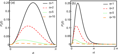
Figure 2: Reduction of the intermediate-level occupancy by modifying the dressed state, see. Eqs. (IV)-(31). (a) The first example (a) shown in Table I. (b) The second example (b) shown in the Table.

Now, it is straightforward to see that the population on the intermediate level $|2\rangle$ changes from $P_{2}(t)=\sin^{2}\vartheta(t)\cos^{2}\vartheta(t)$ [see Eq. (9)] to

$$P_{2}^{\prime}(t)=\frac{\cos^{2}\vartheta(t)}{\eta^{2}(t)+\cot^{2}\vartheta(t)}.$$ (30)

As long as $|\eta(t)|>1$, the above strategy will lead to reduction of the population on $|2\rangle$ with the ratio

$$\frac{P_{2}^{\prime}(t)}{P_{2}(t)}=\frac{1}{\eta^{2}(t)\sin^{2}\vartheta(t)+\cos^{2}\vartheta(t)}.$$ (31)

For the case that $\eta$ is a constant, the maximal inhibition rate is achieved at a time point with $\vartheta=\frac{\pi}{4}$, wherein the maximal occupancy on the level $|2\rangle$ just right happens. The value of the rate there is obtained as $P_{2}^{\prime}/P_{2}=2/(1+\eta^{2})$. As is illustrated in Fig. 2, sizable reduction of the occupancy of the intermediate level could be achieved for the driving protocol by adjusting the factor $\eta$.

V Conclusion

In summary, we have proposed a nonadiabatic driving scheme to realize the stimulated Raman process. The scheme applies no auxiliary coupling field but only the pump and the Stokes lasers to the $\Lambda$-type system with one-photon resonance. The nonadiabatic effect is shown to play a decisive role in the state transfer protocol and some typical Raman nonadiabatic passages generated by the scheme are illustrated. We further investigate the interplay between the present scheme and the STIRSAP based on the transitionless tracking algorithm. By incorporating the latter technology, we show that alternative nonadiabatic passages with less occupancy of the intermediate level could be constructed.

References

- (1) U. Gaubatz, P. Rudecki, M. Becker, S. Schiemann, M. Külz, and K. Bergmann, Chem. Phys. Lett. 149, 463 (1988).
- (2) U. Gaubatz, P. Rudecki, S. Schiemann, and K. Bergmann, J. Chem. Phys. 92, 5363 (1990).
- (3) K. Bergmann, H. Theuer, and B. W. Shore, Rev. Mod. Phys. 70, 1003 (1998).
- (4) N.V. Vitanov, K.A. Suominen, and B.W. Shore, J. Phys. B 32, 4535 (1999).
- (5) N.V. Vitanov, T. Halfmann, B. W. Shore, and K. Bergmann, Annu. Rev. Phys. Chem. 52, 763 (2001).
- (6) P. Král, I. Thanopoulos, and M. Shapiro, Rev. Mod. Phys. 79, 53 (2007).
- (7) M. Demirplak and S.A. Rice, J. Phys. Chem. A 107, 9937 (2003).
- (8) M. Demirplak and S.A. Rice, J. Phys. Chem. B 109, 6838 (2005).
- (9) M. Berry, J. Phys. A: Math. Theor. 42, 365303 (2009).
- (10) X. Chen, I. Lizuain, A. Ruschhaupt, D. Guéry-Odelin, and J.G. Muga, Phys. Rev. Lett. 105, 123003 (2010).
- (11) X. Chen and J. G. Muga, Phys. Rev. A 86, 033405 (2012).
- (12) L. Giannelli and E. Arimondo, Phys. Rev. A 89, 033419 (2014).
- (13) X.-K. Song, Q. Ai, J. Qiu, and F.-G. Deng, Phys. Rev. A 93, 052324 (2016).
- (14) A. Baksic, H. Ribeiro, and A. A. Clerk, Phys. Rev. Lett. 116, 230503 (2016).
- (15) Y.-C. Li and X. Chen, Phys. Rev. A 94, 063411 (2016).
- (16) F. Petiziol, B. Dive, F. Mintert, and S. Wimberger, Phys. Rev. A 98, 043436 (2018).
- (17) G. Yang, W. Li, and L.-X. Cen, Chin. Phys. Lett. 35, 013201 (2018).
- (18) W. Li and L.-X. Cen, Ann. Phys. 389, 1 (2018).
- (19) W. Li and L.-X. Cen, Quantum Inf. Process. 17, 97 (2018).
- (20) P.-J. Zhao, W. Li, H. Cao, S.-W. Yao, and L.-X. Cen, Phys. Rev. A 98, 022136 (2018).
- (21) H.R. Lewis Jr., Phys. Rev. Lett. 18, 510 (1967).
- (22) H.R. Lewis Jr., W.B. Riesenfeld, J. Math. Phys. 10, 1458 (1969).
- (23) N.V. Vitanov and S. Stenholm, Phys. Rev. A 55, 648 (1997).
- (24) J. Klein, F. Beil, and T. Halfmann, Phys. Rev. A 78, 033416 (2008).
- (25) G.G. Grigoryan, G.V. Nikoghosyan, T. Halfmann, Y.T. Pashayan-Leroy, C. Leroy, and S. Guérin, Phys. Rev. A 80, 033402 (2009).
- (26) Q. Shi and E. Geva, J. Chem. Phys. 119, 11773 (2003).
- (27) P.A. Ivanov, N.V. Vitanov, and K. Bergmann, Phys. Rev. A 70, 063409 (2004).
- (28) M. Scala, B. Militello, A. Messina, J. Piilo, and S. Maniscalco, Phys. Rev. A 75, 013811 (2007).
- (29) M. Scala, B. Militello, A. Messina, S. Maniscalco, J. Piilo, and K.-A. Suominen, Phys. Rev. A 77, 043827 (2008).
- (30) M. Scala, B. Militello, A. Messina, and N.V. Vitanov, Phys. Rev. A 81, 053847 (2010).
- (31) M. Scala, B. Militello, A. Messina, and N.V. Vitanov, Phys. Rev. A 83, 012101 (2011).