Adaptive spline fitting with particle swarm optimization

Abstract

In fitting data with a spline, finding the optimal placement of knots can significantly improve the quality of the fit. However, the challenging high-dimensional and non-convex optimization problem associated with completely free knot placement has been a major roadblock in using this approach. We present a method that uses particle swarm optimization (PSO) combined with model selection to address this challenge. The problem of overfitting due to knot clustering that accompanies free knot placement is mitigated in this method by explicit regularization, resulting in a significantly improved performance on highly noisy data. The principal design choices available in the method are delineated and a statistically rigorous study of their effect on performance is carried out using simulated data and a wide variety of benchmark functions. Our results demonstrate that PSO-based free knot placement leads to a viable and flexible adaptive spline fitting approach that allows the fitting of both smooth and non-smooth functions.

I Introduction

A spline of order $k$ is a piecewise polynomial function that obeys continuity conditions on its value and its first $k-2$ derivatives at the points, called knots, where the pieces join deBoor . Splines play an important role in nonparametric regression wegman1983splines ; wahba1990spline ; hardle1990applied , simply called curve fitting when the data is one dimensional, where the outcome is not assumed to have a predetermined form of functional dependence on the predictor.

It has long been recognized wold1974spline ; burchard1974splines ; jupp1978approximation ; luo1997hybrid that the quality of a spline fit depends significantly on the locations of the knots defining the spline. Determining the placement of knots that is best adapted to given data has proven to be a challenging non-linear and non-convex, not to mention high-dimensional, optimization problem that has resisted a satisfactory solution.

A diverse set of methods have been proposed that either attempt this optimization problem head-on or solve an approximation to it in order to get a reasonable solution. In the latter category, methods based on knot insertion and deletion smith1982curve ; lyche1988data ; friedman1989flexible ; friedman1991 ; stone1997polynomial have been studied extensively. In these methods, one starts with a fixed set of sites for knots and performs a step-wise addition or removal of knots at these sites. The best number of knots is determined by a model selection criterion such as Generalized Cross Validation (GCV) luo1997hybrid ; golub1979generalized . Step-wise change in knot placement is not an efficient exploration of the continuous space of possible knot positions and the end result, while computationally inexpensive to obtain and tractable to mathematical analysis, is not necessarily the best possible zhou2001spatially . Another approach explored in the literature is the two-stage framework in which the first stage identifies a subset of active or dominant knots and the second stage merges them in a data dependent way to obtain a reduced set of knots park2007b ; kang2015knot ; luo2019knot . These methods have shown good performance for low noise applications.

In attempts at solving the optimization challenge directly, general purpose stochastic optimization algorithms (metaheuristics) such as Genetic Algorithm (GA) geneticalgo , Artificial Immune System (AIS) ulker2009automatic or those based on Markov Chain Monte Carlo (MCMC) green1995reversible , have been studied pittman2002adaptive ; dimatteo2001bayesian ; YOSHIMOTO2003751 ; miyata2003adaptive . These methods have proven quite successful in solving many challenging high-dimensional optimization problems in other fields and it is only natural to employ them for the problem of free knot placement. However, GA and AIS are more suited to discrete optimization problems rather than the inherently continuous one in knot optimization, and MCMC is computationally expensive. Thus, there is plenty of scope for using other metaheuristics to find better solutions.

It was shown in galvez2011efficient , and independently in mohanty2012particle , that Particle Swarm Optimization (PSO) PSO , a relatively recent entrant to the field of nature inspired metaheuristics such as GA, is a promising method for the free knot placement problem. PSO is governed by a much smaller set of parameters than GA or MCMC and most of these do not appear to require much tuning from one problem to another. In fact, as discussed later in the paper, essentially two parameters are all that need to be explored to find a robust operating point for PSO.

An advantage of free knot placement is that a subset of knots can move close enough to be considered as a single knot with a higher multiplicity. A knot with multiplicity $>1$ can be used to construct splines that can fit curves with discontinuities. Thus, allowing knots to move and merge opens up the possibility of modeling even non-smooth curves. That PSO can handle regression models requiring knot merging was demonstrated in galvez2011efficient albeit for examples with very low noise levels.

It was found in SEECR-PhysRevD.96.102008 , and later in a simplified model problem mohanty2018swarm , that the advantage engendered by free knot placement turns into a liability as the level of noise increases: knots can form spurious clusters to fit outliers arising from noise, producing spikes in the resulting estimate and making it worse than useless. This problem was found to be mitigated mohanty2018swarm by introducing a suitable regulator ruppert2003semiparametric . Regularization has also been used in combination with knot addition luo1997hybrid but its role there – suppression of numerical instability arising from a large numbers of knots – is very different.

The progress on free knot placement described above has happened over decades and in somewhat isolated steps that were often limited by the available computing power. However, the tremendous growth in computing power and the development of more powerful metaheuristics has finally brought us to the doorstep of a satisfactory resolution of this problem, at least for one-dimensional regression.

In this paper, we combine PSO based knot placement with regularization into a single algorithm for adaptive spline fitting. The algorithm, called Swarm Heuristics based Adaptive and Penalized Estimation of Splines (SHAPES), has the flexibility to fit non-smooth functions as well as smooth ones without any change in algorithm settings. It uses model selection to determine the best number of knots, and reduces estimation bias arising from the regularization using a least squares derived rescaling. Some of the elements of SHAPES outlined above were explored in mohanty2018swarm in the context of a single example with a simple and smooth function. However, the crucial feature of allowing knots to merge was missing there along with the step of bias reduction. (The bias reduction step does not seem to have been used elsewhere to the best of our knowledge.)

Various design choices involved in SHAPES are identified clearly and their effects are examined using large-scale simulations and a diverse set of benchmark functions. Most importantly, SHAPES is applied to data with a much higher noise level than has traditionally been considered in the field of adaptive spline fitting and found to have promising performance. This sets the stage for further development of the adaptive spline methodology for new application domains.

The rest of the paper is organized as follows. Sec. II provides a brief review of pertinent topics in spline fitting. The PSO metaheuristic and the particular variant used in this paper are reviewed in Sec. III. Details of SHAPES are described in Sec. IV along with the principal design choices. The setup used for our simulations is described in Sec. V. Computational aspects of SHAPES are addressed in Sec. VI. This is followed by the presentation of results in Sec. VII. Our conclusions are summarized in Sec. VIII.

II Fitting splines to noisy data

In this paper, we consider the one-dimensional regression problem

$$y_{i} = f(x_{i})+\epsilon_{i}\;,$$ (1)

$i=0,1,\ldots,N-1$, $x_{0}=0$, $x_{N-1}=1$, $x_{i+1}>x_{i}$, with $f(x)$ unknown and $\epsilon_{i}$ drawn independently from $N(0,1)$. The task is to find an estimate $\widehat{f}(x)$, given $\{y_{i}\}$, of $f(x)$.

To obtain a non-trivial solution, the estimation problem must be regularized by restricting $\widehat{f}(x)$ to some specified class of functions. One reasonable approach is to require that this be the class of “smooth” functions, and obtain the estimate as the solution of the variational problem,

$$\widehat{f} = \operatornamewithlimits{arg\ min}_{f}\left[\sum_{i=0}^{N-1}\left(y_{i}-f(x_{i})\right)^{2}+\lambda\int_{0}^{1}dx\left(f^{\prime\prime}(x)\right)^{2}\right]\;.$$ (2)

It can be shown that the solution belongs to the space of cubic splines defined by $\{x_{i}\}$ as the set of knots. Consequently, $\widehat{f}$ is known as the smoothing spline estimate wahba1990spline ; reinsch1967smoothing . In Eq. 2, the first term on the right measures the fidelity of the model to the observations and the second term penalizes the “roughness”, measured by the average squared curvature, of the model. The trade-off between these competing requirements is controlled by $\lambda\geq 0$, called the regulator gain or smoothing parameter.

The best choice for $\lambda$ is the principle issue in practical applications of smoothing spline. The use of GCV to adaptively determine the value of $\lambda$ was introduced in craven1978smoothing and is used, for example, in the implementation of smoothing spline in the R R-software stats package. A scalar $\lambda$, adaptively selected or otherwise, is not well suited to handle a function with a heterogeneous roughness distribution across its domain. The use of a spatially adaptive gain function, $\lambda(x)$, has been investigated in different forms wahba_donoho2002wavelet ; storlie2010locally ; liu2010data ; wang2013smoothing to address this issue.

A different regularization approach is to eschew an explicit penalty term and regularize the fitting problem by restricting the number of knots to be $\ll N$. This leads to the regression spline wold1974spline estimate in which $\widehat{f}(x)$ is represented as a linear combination of a finite set of basis functions – the so-called B-spline functions deBoor ; curry1947spline being a popular choice – that span the space of splines associated with the chosen knot sequence and polynomial order. Different methods for adaptive selection of the number of knots, which is the main free parameter in regression spline, have been compared in wand2000comparison . The asymptotic properties of smoothing and regression spline estimates have been analyzed theoretically in claeskens2009asymptotic .

Smoothing and regression splines are hybridized in the penalized spline ruppert2003semiparametric ; eilers1996flexible ; eilers2015twenty approach: the deviation of the spline model from the data is measured by the least squares function as in the first term of Eq. 2 but the penalty becomes a quadratic form in the coefficients of the spline in the chosen basis set. As in the case of smoothing spline, adaptive selection of the scalar regulator gain can be performed using GCV ruppert2003semiparametric and locally adaptive gain coefficients have been proposed in ruppert2000theory ; krivobokova2008fast ; scheipl2009locally ; yang2017adaptive . The performance of alternatives to GCV for selection of a scalar regulator gain have been investigated and compared in krivobokova2013smoothing .

While penalized spline is less sensitive to the number of knots, it is still a free parameter of the algorithm that must be specified. Joint adaptive selection of the number of knots and regulator gain has been investigated in luo1997hybrid ; ruppert2002selecting using GCV. Other model selection methods can also be used for adaptive determination of the number of knots (see Sec. II.3).

II.1 B-spline functions

Given a set of $M$ knots $\overline{b}=(b_{0},b_{1},\ldots,b_{M-1})$, $b_{i}\in[0,1]$, $b_{i+1}>b_{i}$, and given order $k$ of the spline polynomials, the set of splines that interpolates $\{(y_{i},b_{i})\}$, $y_{i}\in\mathbb{R}$, forms a linear vector space of dimensionality $M+k-2$. A convenient choice for a basis of this vector space is the set of B-spline functions curry1947spline .

In this paper, we need B-spline functions for the more general case of a knot sequence $\overline{\tau}=(\tau_{0},\tau_{1},\ldots,\tau_{P-1})$, $\tau_{i+1}\geq\tau_{i}$ with $P>M$ knots, in which a knot can appear more than once. The number of repetitions of any knot cannot be greater than $k$. Also, $\tau_{j}=b_{0}$ for $0\leq j\leq k-1$, and $\tau_{j}=b_{M-1}$ for $P-k\leq j\leq P-1$. The span of B-spline functions defined over a knot sequence with repetitions can contain functions that have jump discontinuities in their values or in their derivatives. (The dimensionality of the span is $P-k$.)

The Cox-de Boor recursion relations DEBOOR197250 given below provide an efficient way to compute the set of B-spline functions, $\{B_{i,k}(x;\overline{\tau})\}$, for any given order. The recursions start with B-splines of order 1, which are piecewise constant functions

$$B_{j,1}(x;\overline{\tau}) = \left\{\begin{array}[]{cc}1,&\tau_{j}\leq x<\tau_{j+1}\\ 0&{\rm else}\end{array}\right.\;.$$ (5)

For $2\leq k^{\prime}\leq k$,

$$B_{j,k^{\prime}}(x) = \omega_{j,k^{\prime}}(x)B_{j,k^{\prime}-1}(x)+\gamma_{j+1,k^{\prime}}(x)B_{j+1,k^{\prime}-1}(x)\;,$$ (6)

$$\omega_{j,k^{\prime}}(x) = \left\{\begin{array}[]{cc}\frac{x-\tau_{j}}{\tau_{j+k^{\prime}-1}-\tau_{j}}\;,&\tau_{j+k^{\prime}-1}\neq\tau_{j}\\ 0\;,&\tau_{j+k^{\prime}-1}=\tau_{j}\end{array}\right.\;,$$ (9)

$$\gamma_{j,k^{\prime}}(x) = \left\{\begin{array}[]{cc}1-\omega_{j,k^{\prime}}(x)\;,&\tau_{j+k^{\prime}-1}\neq\tau_{j}\\ 0\;,&\tau_{j+k^{\prime}-1}=\tau_{j}\end{array}\right.\;.$$ (12)

In the recursion above, $0\leq j\leq P-k^{\prime}-1$. Fig. 1 provides an illustration of B-spline functions.

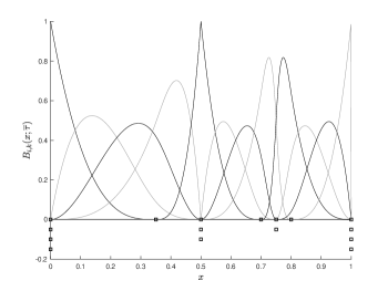
Figure 1: Cubic B-spline functions $\{B_{i,4}(x;\overline{\tau})\}$, $i=0,1,\ldots,11$, for an arbitrary choice of $16$ knots ($\overline{\tau}$) marked by squares. For visual clarity, alternate B-spline functions are shown in black and gray. Knots with multiplicity $>1$ result in B-splines that are discontinuous in value or derivatives.

The regression spline method is elegantly formulated in terms of B-spline functions. The estimate is assumed to belong to the parametrized family of linearly combined B-spline functions,

$$f(x;\overline{\alpha},\overline{\tau}) = \sum_{j=0}^{P-k-1}\alpha_{j}B_{j,k}(x_{i};\overline{\tau})\;,$$ (13)

where $\overline{\alpha}=(\alpha_{0},\alpha_{1},\ldots,\alpha_{P-k-1})$. The least-squares estimate is given by $\widehat{f}(x)=f(x;\widehat{\alpha},\widehat{\tau})$, where $\widehat{\alpha}$ and $\widehat{\tau}$ minimize

$$L(\overline{\alpha},\overline{\tau}) = \sum_{i=0}^{N-1}\left(y_{i}-f(x_{i};\overline{\alpha},\overline{\tau})\right)^{2}\;.$$ (14)

II.2 Regression and penalized spline with free knot placement

The penalized spline estimate is found by minimizing

$$L_{\lambda}(\overline{\alpha},\overline{\tau}) = L(\overline{\alpha},\overline{\tau})+\lambda R(\overline{\alpha})\;,$$ (15)

over the spline coefficients (c.f. Eq. 13), where $R(\overline{\alpha})$ is the penalty, while keeping the number of knots and knot locations fixed. In this paper, we choose

$$R(\overline{\alpha}) = \sum_{j=0}^{P-k-1}\alpha_{j}^{2}\;,$$ (16)

for reasons explained below.

Formally, the penalty function can be derived by substituting Eq. 13 in the roughness penalty. This would lead to a quadratic form similar to the penalty in Eq. 16 but with a kernel matrix that is not the identity matrix ramsay_silverman_functional . The elements of this matrix would be Euclidean inner products of B-spline derivatives. However, using such a penalty adds a substantial computational burden in free knot placement because it has to be recomputed every time the knot placement changes. Computational aspects of this problem are discussed in eilers1996flexible , where a simplified form of the roughness penalty is used that is based on the differences of coefficients of adjacent B-splines. This is a good approximation for the case considered in eilers1996flexible of a large number of fixed knots and closely spaced B-splines, but not necessarily for free knots that may be small in number and widely spread out. Another perhaps more important consideration is that repeated knots in free knot placement result in B-splines with discontinuous derivatives. This makes the kernel matrix particularly challenging for numerical evaluation and increases code complexity. In this paper, we avoid the above issues by using the simple form of the penalty function in Eq. 16 and leave the investigation of more appropriate forms to future work. We note that the exploration of innovative penalty functions is an active topic of research (e.g., lindstrom1999penalized ; eilers2015twenty ; goepp2018spline ).

While the reduction of the number of knots in regression spline coupled with the explicit regularization of penalized spline reduces overfitting, the fit is now sensitized to where the knots are placed. Thus, the complete method involves the minimization of $L_{\lambda}(\overline{\alpha},\overline{\tau})$ (c.f., Eq. 15) over both $\overline{\alpha}$ and $\overline{\tau}$. (The method of regression spline with knot optimization and explicit regularization will be referred to as adaptive spline in the following.)

Minimization of $L_{\lambda}$ over $\overline{\alpha}$ and $\overline{\tau}$ can be nested as follows.

$$\min_{\overline{\tau},\overline{\alpha}}L_{\lambda}(\overline{\alpha},\overline{\tau}) = \min_{\overline{\tau}}\left(\min_{\overline{\alpha}}L_{\lambda}(\overline{\alpha},\overline{\tau})\right)\;.$$ (17)

The solution, $\widehat{\alpha}(\overline{\tau})$, of the inner minimization is expressed in terms of the $(P-k)$-by-$N$ matrix ${\bf B}(\overline{\tau})$, with

$$B_{m,n}(\overline{\tau}) = B_{m,k}(x_{n};\overline{\tau})\;,$$ (18)

as

$$\widehat{\alpha}(\overline{\tau}) = \overline{y}{\bf B}^{T}{\bf G}^{-1}\;,$$ (19)

$${\bf G} = {\bf B}{\bf B}^{T}+\lambda{\bf I}\;,$$ (20)

where ${\bf I}$ is the $(P-k)$-by-$(P-k)$ identity matrix. The outer minimization over $\overline{\tau}$ of

$$F_{\lambda}(\overline{\tau}) = L_{\lambda}(\widehat{\alpha}(\overline{\tau}),\overline{\tau})\;,$$ (21)

needs to be performed numerically.

Due to the fact that freely moveable knots can coincide, and that this produces discontinuities in B-spline functions as outlined earlier, curve fitting by adaptive spline can accommodate a broader class of functions – smooth with localized discontinuities – than smoothing or penalized spline.

The main bottleneck in implementing the adaptive spline method is the global minimization of $F_{\lambda}(\overline{\tau})$ since it is a high-dimensional non-convex function having multiple local minima. Trapping by local minima renders greedy methods ineffective and high dimensionality makes a brute force search for the global minimum computationally infeasible. This is where PSO enters the picture and, as shown later, offers a way forward.

II.3 Model selection

In addition to the parameters $\overline{\alpha}$ and $\overline{\tau}$, adaptive spline has two hyper-parameters, namely the regulator gain $\lambda$ and the number of interior knots $P-2(k-1)$, that affect the outcome of fitting. Model selection methods can be employed to fix these hyper-parameters based on the data.

In this paper, we restrict ourselves to the adaptive selection of only the number of knots. This is done by minimizing the Akaike Information Criterion (AIC) akaike1998information : For a regression model with $K$ parameters $\overline{\theta}=(\theta_{0},\theta_{1},\ldots,\theta_{K-1})$,

$${\rm AIC} = 2K-2\max_{\overline{\theta}}\ln\left(\Lambda(\overline{\theta})\right)\;,$$ (22)

where $\Lambda(\overline{\theta})$ is the likelihood function. The specific expression for AIC used in SHAPES is provided in Sec. IV.

III Particle swarm optimization

Under the PSO metaheuristic, the function to be optimized (called the fitness function) is sampled at a fixed number of locations (called particles). The set of particles is called a swarm. The particles move in the search space following stochastic iterative rules called dynamical equations. The dynamical equations implement two essential features called cognitive and social forces. They serve to retain “memories” of the best locations found by the particle and the swarm (or a subset thereof) respectively.

Since its introduction by Kennedy and Eberhart PSO , the PSO metaheuristic has expanded to include a large diversity of algorithms engelbrecht2005fundamentals . In this paper, we consider the variant called local-best (or lbest) PSO lbestTopology . We begin with the notation normandin2018particle for describing lbest PSO.

• $F(x)$: the scalar fitness function to be minimized, with $x=(x^{1},x^{2},\ldots,x^{d})\in\mathbb{R}^{d}$. In our case, $x$ is $\overline{\tau}$, $F$ is $F_{\lambda}(\overline{\tau})$ (c.f., Eq. 21), and $d=P-2(k-1)$.

• $\mathcal{S}\subset\mathbb{R}^{d}$: the search space defined by the hypercube $a^{j}\leq x^{j}\leq b^{j}$, $=1,2,\ldots,d$ in which the global minimum of the fitness function must be found.

• $N_{p}$: the number of particles in the swarm.

• $x_{i}[k]\in\mathbb{R}^{d}$: the position of the $i^{\rm th}$ particle at the $k^{\rm th}$ iteration.

• $v_{i}[k]\in\mathbb{R}^{d}$: a vector called the velocity of the $i^{\rm th}$ particle that is used for updating the position of a particle.

• $p_{i}[k]\in\mathbb{R}^{d}$: the best location found by the $i^{\rm th}$ particle over all iterations up to and including the $k^{\rm th}$. $p_{i}[k]$ is called the personal best position of the $i^{\rm th}$ particle.

  $$F(p_{i}[k]) = \min_{1\leq j\leq k}F(x_{i}[j])\;.$$ (23)

• $n_{i}[k]$: a set of particles, called the neighborhood of particle $i$, $n_{i}[k]\subseteq\{1,2,\ldots,N_{p}\}\setminus\{i\}$. There are many possibilities, called topologies, for the choice of $n_{i}[k]$. In the simplest, called the global best topology, every particle is the neighbor of every other particle: $n_{i}[k]=\{1,2,\ldots,N_{p}\}\setminus\{i\}$. The topology used for lbest PSO in this paper is described later.

• $l_{i}[k]\in\mathbb{R}^{d}$: the best location among the particles in $n_{i}[k]$ over all iterations up to and including the $k^{\rm th}$. $l_{i}[k]$ is called the local best for the $i^{\rm th}$ particle.

  $$F(l_{i}[k]) = \min_{j\in\{i\}\cup n_{i}[k]}F(p_{j}[k])\;.$$ (24)

• $p_{g}[k]\in\mathbb{R}^{d}$: The best location among all the particles in the swarm, $p_{g}[k]$ is called the global best.

  $$F(p_{g}[k]) = \min_{1\leq i\leq N_{p}}F(p_{i}[k])\;.$$ (25)

The dynamical equations for lbest PSO are as follows.

$$v_{i}[k+1] = w[k]v_{i}[k]+c_{1}(p_{i}[k]-x_{i}[k]){\bf r}_{1}+$$ (26)

$$c_{2}(l_{i}[k]-x_{i}[k]){\bf r}_{2}\;,$$

$$x_{i}[k+1] = x_{i}[k]+z_{i}[k+1]\;,$$ (27)

$$z^{j}_{i}[k] = \left\{\begin{array}[]{cc}v_{i}^{j}[k]\,,&-v_{\rm max}^{j}\leq v_{i}^{j}[k]\leq v_{\rm max}^{j}\\ -v_{\rm max}^{j}\,,&v_{i}^{j}[k]<-v_{\rm max}^{j}\\ v_{\rm max}^{j}\,,&v_{i}^{j}[k]>v_{\rm max}^{j}\end{array}\right.\;.$$ (31)

Here, $w[k]$ is a deterministic function known as the inertia weight, $c_{1}$ and $c_{2}$ are constants, and ${\bf r}_{i}$ is a diagonal matrix with iid random variables having a uniform distribution over $[0,1]$. Limiting the velocity as shown in Eq. 31 is called velocity clamping.

The iterations are initialized at $k=1$ by independently drawing (i) $x_{i}^{j}[1]$ from a uniform distribution over $[a^{j},b^{j}]$, and (ii) $v_{i}^{j}[1]$ from a uniform distribution over $[a^{j}-x_{i}^{j}[1],b^{j}-x_{i}^{j}[1]]$. For termination of the iterations, we use the simplest condition: terminate when a prescribed number ${N_{\rm iter}}$ of iterations are completed. The solutions found by PSO for the minimizer and the minimum value of the fitness are $p_{g}[N_{\rm iter}]$ and $F(p_{g}[N_{\rm iter}])$ respectively. Other, more sophisticated, termination conditions are available engelbrecht2005fundamentals , but the simplest one has served well across a variety of regression problems in our experience.

The second and third terms on the RHS of Eq. 26 are the cognitive and social forces respectively. On average they attract a particle towards its personal and local bests, promoting the exploitation of an already good solution to find better ones nearby. The term containing the inertia weight, on the other hand, promotes motion along the same direction and allows a particle to resist the cognitive and social forces. Taken together, the terms control the exploratory and exploitative behaviour of the algorithm. We allow the inertia weight $w[k]$ to decrease linearly with $k$ from an initial value $w_{\rm max}$ to a final value $w_{\rm min}$ in order to transition PSO from an initial exploratory to a final exploitative phase.

For the topology, we use the ring topology with $2$ neighbors in which

$$n_{i}[k]=\left\{\begin{array}[]{cc}\{i-1,i+1\}\;,&i\notin\{1,N_{p}\}\\ \{N_{p},i+1\}\;,&i=1\\ \{i-1,1\}\;,&i=N_{p}\end{array}\right.\;.$$ (35)

The local best, $l_{i}[k]$, in the $k^{\rm th}$ iteration is updated after evaluating the fitnesses of all the particles. The velocity and position updates given by Eq. 26 and Eq. 27 respectively form the last set of operations in the $k^{\rm th}$ iteration.

To handle particles that exit the search space, we use the “let them fly” boundary condition under which a particle outside the search space is assigned a fitness value of $\infty$. Since both $p_{i}[k]$ and $l_{i}[k]$ are always within the search space, such a particle is eventually pulled back into the search space by the cognitive and social forces.

III.1 PSO tuning

Stochastic global optimizers, including PSO, that terminate in a finite number of iterations do not satisfy the conditions laid out in solis1981minimization for convergence to the global optimum. Only the probability of convergence can be improved by tuning the parameters of the algorithm for a given optimization problem.

In this sense, most of the parameters involved in PSO are found to have fairly robust values when tested across an extensive suite of benchmark fitness functions bratton2007defining . Based on widely prevalent values in the literature, these are: $N_{p}=40$, $c_{1}=c_{2}=2.0$, $w_{\rm max}=0.9$, $w_{\rm min}=0.4$, and $v_{\rm max}^{j}=0.5[b^{j}-a^{j}]$.

Typically, this leaves the maximum number of iterations, $N_{\rm iter}$, as the principal parameter that needs to be tuned. However, for a given $N_{\rm iter}$, the probability of convergence can be increased by the simple strategy of running multiple, independently initialized runs of PSO on the same fitness function and choosing the best fitness value found across the runs. The probability of missing the global optimum decreases exponentially as $(1-P_{\rm conv})^{N_{\rm runs}}$, where $P_{\rm conv}$ is the probability of successful convergence in any one run and $N_{\rm runs}$ is the number of independent runs.

Besides $N_{\rm iter}$, therefore, $N_{\rm runs}$ is the remaining parameter that should be tuned. If the independent runs can be parallelized, $N_{\rm runs}$ is essentially fixed by the available number of parallel workers although this should not be stretched to the extreme. If too high a value of $N_{\rm runs}$ is needed in an application (say $N_{\rm runs}\geq 8$), it is usually an indicator that $P_{\rm conv}$ should be increased by tuning the other PSO parameters or by exploring a different PSO variant. In this paper, we follow the simpler way of tuning $N_{\rm runs}$ by setting it to $N_{\rm runs}=4$, the typical number of processing cores available in a high-end desktop.

IV SHAPES algorithm

The SHAPES algorithm is summarized in the pseudo-code given in Fig. 2. The user specified parameters of the algorithm are (i) the number, $N_{\rm runs}$, of PSO to use per data realization; (ii) the number of iterations, $N_{\rm iter}$, to termination of PSO; (iii) the set of models, $\mathbb{N}_{\rm knots}$, over which AIC based model selection (see below) is used; (iv) the regulator gain $\lambda$. Following the standard initialization condition for PSO (c.f., Sec. III), the initial knots for each run of PSO are drawn independently from a uniform distribution over $[0,1]$.

Input:

$\bullet$ $\overline{y}\leftarrow$ Data

$\bullet$ $N_{\rm runs}\leftarrow$ Number of PSO runs

$\bullet$ $N_{\rm iter}\leftarrow$ Maximum number of iterations

$\bullet$ $\mathbb{N}_{\rm knots}\leftarrow\{M_{1},M_{2},\ldots,M_{\rm max}\}$; Number of knots (not counting repetitions)

$\bullet$ $\lambda\leftarrow$ Regulator gain

Execute:

for $M\in\mathbb{N}_{\rm knots}$ do$\triangleright$ Loop over models

     for $r\in\{1,2,\ldots,N_{\rm runs}\}$ do $\triangleright$ (Parallel) loop over PSO runs

         $\widehat{\tau}(r)\leftarrow$ $\operatornamewithlimits{arg\ min}_{\overline{\tau}}F_{\lambda}(\overline{\tau})$ using PSO $\triangleright$ Best location

         $\widehat{\alpha}(r)\leftarrow$ B-spline coefficients corresponding to $\widehat{\tau}(r)$

         $F(M,r)\leftarrow$ $F_{\lambda}(\widehat{\tau}(r))$ $\triangleright$ Best fitness value

     end for

     $r_{M}\leftarrow\operatornamewithlimits{arg\ min}_{r}F(M,r)$ $\triangleright$ Best PSO run

     ${\rm AIC}(M)\leftarrow{\rm AIC}$ for $F(M,r_{M})$ (c.f., Eq. 36)

     $\widehat{f}(M)\leftarrow$ Estimated function corresponding to $\widehat{\tau}(r_{M})$ and $\widehat{\alpha}(r_{M})$

end for

$M_{\rm best}\leftarrow\operatornamewithlimits{arg\ min}_{M}{\rm AIC}(M)$ $\triangleright$ Model with lowest AIC

$\widehat{f}\leftarrow$ $\widehat{f}(M_{\rm best})$

$\widehat{f}\leftarrow$ Bias corrected $\widehat{f}$ (c.f., Sec. IV.1)

Output:

$\bullet$ $M_{\rm best}$$\triangleright$ Best model

$\bullet$ Estimated, bias-corrected $\widehat{f}$ $\triangleright$ Estimated function from best model

$\bullet$ $F(M_{\rm best},r_{M_{\rm best}})$ $\triangleright$ Fitness of best model

Figure 2: Pseudo-code for the SHAPES algorithm. All quantities with parenthesized integer arguments stand for arrays, with the argument as the array index.

A model in SHAPES is specified by the number of non-repeating knots. For each model $M\in\mathbb{N}_{\rm knots}$, $F(M,r_{M})$ denotes the fitness value, where $1\leq r_{M}\leq N_{\rm runs}$ is the best PSO run. The AIC value for the model is given by

$${\rm AIC} = 4M+F(M,r_{M})\;,$$ (36)

which follows from the number of optimized parameters being $2M$ (accounting for both knots and B-spline coefficients) and the log-likelihood being proportional to the least squares function for the noise model used here. (Additive constants that do not affect the minimization of AIC have been dropped.)

The algorithm acts on given data $\overline{y}$ to produce (i) the best fit model $M_{\rm best}\in\mathbb{N}_{\rm knots}$; (ii) the fitness value associated with the best fit model; (iii) the estimated function $\widehat{f}$ from the best fit model. The generation of $\widehat{f}$ includes a bias correction step described next.

IV.1 Bias correction

The use of a non-zero regulator gain leads to shrinkage in the estimated B-spline coefficients. As a result, the corresponding estimate, $\widehat{f}$, has a systematic point-wise bias towards zero. A bias correction transformation is applied to $\widehat{f}$ as follows.

First, the unit norm estimated function $\widehat{u}$ is obtained,

$$\widehat{u} = \frac{\widehat{f}}{\|\widehat{f}\|}\;,$$ (37)

where $\|\widehat{f}\|=[\sum\widehat{f}_{i}^{2}]^{1/2}$ is the $L_{2}$ norm.

Next, a scaling factor $A$ is estimated as

$$A = \operatornamewithlimits{arg\ min}_{a}\sum_{i=0}^{N-1}\left(y_{i}-a\widehat{u}\right)^{2}\;.$$ (38)

The final estimate is given by $\widehat{f}=A\widehat{u}$.

As discussed earlier in Sec. II.2 (c.f. Eq. 15 and Eq. 16), the penalty used in this paper is one among several alternatives available in the literature. For some forms of the penalty, there need not be any shrinkage in the B-spline coefficients and the bias correction step above would be unnecessary.

IV.2 Knot merging and dispersion

In both of the mappings described in Sec. IV.3, it is possible to get knot sequences in which a subset $(\tau_{i},\tau_{i+1},\ldots,\tau_{i+m-1})$ of $1<m\leq M-2$ of interior knots falls within an interval $(x_{j},x_{j+1})$ between two consecutive predictor values. There are two possible options to handle such a situation.

• Heal: Overcrowded knots are dispersed such that there is only one knot between any two consecutive predictor values. This can be done iteratively by moving a knot to the right or left depending on the difference in distance to the corresponding neighbors.

• Merge: All the knots in an overcrowded set are made equal to the rightmost knot $\tau_{i+m-1}$ until its multiplicity saturates at $k$. The remaining knots, $\tau_{i}$ to $\tau_{i+m-1-k}$, are equalized to the remaining rightmost knot $\tau_{i+m-1-k}$ until its multiplicity staturates to $k$, and so on. (Replacing rightmost by leftmost when merging is an equally valid alternative.) Finally, if more than one set of merged knots remain within an interval $(x_{j},x_{j+1})$, they are dispersed by healing.

If only healing is used, SHAPES cannot fit curves that have jump discontinuities in value or derivatives. Therefore, if it is known that the unknown curve in the data is free of jump discontinuities, healing acts as an implicit regularization to enforce this condition. Conversely, merging should be used when jump discontinuities cannot be discounted.

It is important to note that in both healing and merging, the number of knots stays fixed at $M+2(k-1)$ where $M\in\mathbb{N}_{\rm knots}$.

IV.3 Mapping particle location to knots

For a given model $M\in\mathbb{N}_{\rm knots}$, the search space for PSO is $M$ dimensional. Every particle location, $\overline{z}=(z_{0},z_{1},\ldots,z_{M-1})$, in this space has to be mapped to an $M+2(k-1)$ element knot sequence $\overline{\tau}$ before evaluating its fitness $F_{\lambda}(\overline{\tau})$.

We consider two alternatives for the map from $\overline{z}$ to $\overline{\tau}$.

• Plain: $\overline{z}$ is sorted in ascending order. After sorting, $k-1$ copies of $z_{0}$ and $z_{M-1}$ are prepended and appended respectively to $\overline{z}$. These are the repeated end knots as described in Sec. II.1.

• Centered-monotonic: In this scheme calvin-siuro , the search space is the unit hypercube: $z_{i}\in[0,1]$, $\forall i$. First, an initial set of $M$ knots is obtained from

  $$z_{0} = \tau_{0}\;,$$ (39)

  $$z_{1\leq i\leq M-2} = \frac{\tau_{i}-\tau_{i-1}}{\tau_{i+1}-\tau_{i-1}}\;,$$ (40)

  $$z_{M-1} = \frac{\tau_{M-1}-\tau_{0}}{1-\tau_{0}}\;.$$ (41)

  This is followed by prepending and appending $k-1$ copies of $\tau_{0}$ and $\tau_{M-1}$ respectively to the initial knot sequence.

In the plain map, any permutation of $\overline{z}$ maps into the same knot sequence due to sorting. This creates degeneracy in $F_{\lambda}$, which may be expected to make the task of global minimization harder for PSO. The centered-monotonic map is designed to overcome this problem: by construction, it assigns a unique $\overline{\tau}$ to a given $\overline{z}$. Moreover, $\overline{\tau}$ is always a monotonic sequence, removing the need for a sorting operation. This map also has the nice normalization that the center of the search space at $z_{i}=0.5$, $1\leq i\leq M-2$, corresponds to uniform spacing of the interior knots.

It should be noted here that the above two maps are not the only possible ones. The importance of the “lethargy theorem” (degeneracy of the fitness function) and using a good parametrization for the knots in regression spline was pointed out by Jupp jupp1978approximation back in $1978$. A logarithmic map for knots was proposed in jupp1978approximation that, while not implemented in this paper, should be examined in future work.

IV.4 Optimization of end knots

When fitting curves to noisy one-dimensional data in a signal processing context, a common situation is that the signal is transient and localized well away from the end points $x_{0}$ and $x_{N-1}$ of the predictor. However, the location of the signal in the data – its time of arrival in other words – may be unknown. In such a case, it makes sense to keep the end knots free and subject to optimization.

On the other hand, if it is known that the curve occupies the entire predictor range, it is best to fix the end knots by keeping $z_{0}$ and $z_{M-1}$ fixed. (This reduces the dimensionality of the search space for PSO by $2$.)

IV.5 Retention of end B-splines

The same signal processing scenario considered above suggests that, for signals that decay smoothly to zero at their start and end, it is best to drop the end B-spline functions because they have a jump discontinuity in value (c.f., Fig 1). In the contrary case, the end B-splines may be retained so that the estimated signal can start or end at non-zero values.

V Simulation study setup

We examine the performance of SHAPES on simulated data with a wide range of benchmark functions. In this section, we present these functions, the simulation protocol used, the metrics for quantifying performance, and a scheme for labeling test cases that is used in Sec. VII. (In the following, the terms “benchmark function” and “benchmark signal” are used interchangeably.)

V.1 Benchmark functions

The benchmark functions used in this study are listed in Table 1 and plotted in Fig. 3.

Table 1: The benchmark functions used in this paper. The sources from which the functions have been obtained are: $f_{1}$ to $f_{3}$ YOSHIMOTO2003751 ; $f_{4}$ dimatteo2001bayesian ; $f_{5}$ denison1998automatic ; li2006bayesian ; $f_{6}$ lee2002algorithms ; $f_{7}$ mohanty2018swarm . Functions $f_{8}$ to $f_{10}$ are introduced here.

Expression	Domain
$f_{1}(x)=90(1+e^{-100(x-0.4)})^{-1}$	$x\in[0,1]$
$f_{2}(x)=\begin{cases}(0.01+(x-0.3)^{2})^{-1}\\ (0.015+(x-0.65)^{2})^{-1}\\ \end{cases}$	$\begin{aligned} 0\leq x<0.6\\ 0.6\leq x\leq 1\end{aligned}$
$f_{3}(x)=100e^{-|10x-5|}+(10x-5)^{5}/500$	$x\in[0,1]$
$f_{4}(x)=\sin(x)+2e^{-30x^{2}}$	$x\in[-2,2]$
$f_{5}(x)=\sin(2x)+2e^{-16x^{2}}+2$	$x\in[-2,2]$
$f_{6}(x)=\begin{cases}4x^{2}(3-4x)\\ \frac{4}{3}x(4x^{2}-10x+7)-\frac{3}{2}\\ \frac{16}{3}x(x-1)^{2}\end{cases}$	$\begin{aligned} 0\leq x<0.5\\ 0.5\leq x<0.75\\ 0.75\leq x\leq 1\end{aligned}$
$\begin{array}[]{rc}f_{7}(x)=B_{3,4}(x;\overline{\tau})\;;&\overline{\tau}=(\tau_{0},\tau_{1},\ldots,\tau_{11})\\ \tau_{i}&=\left\{\begin{array}[]{cc}0.3\;,&0\leq i\leq 2\\ 0.55\;,&8\leq i\leq 10\end{array}\right.\\ (\tau_{3},\ldots,\tau_{7})&=(0.3,0.4,.45,0.5,0.55)\end{array}$	$x\in[0,1]$
$f_{8}(x)=B_{3,4}(x;\overline{\tau})+B_{3,4}(x-0.125;\overline{\tau})$	$x\in[0,1]$
$f_{9}(x)=B_{3,4}(x-0.25,\overline{\tau})+B_{3,4}(x-0.125;\overline{\tau})$	$x\in[0,1]$
$f_{10}(x)=e^{-\frac{(x-0.5)^{2}}{0.125}}\sin\left(10.24\pi(x-0.5)\right)$	$x\in[0,1]$

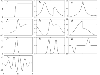
Figure 3: Benchmark functions normalized to have ${\rm SNR}=100$. The function name is indicated in the upper left corner of each panel. The abscissa in each panel is identical to the one showing $f_{10}$.

Function $f_{1}$ has a sharp change but is differentiable everywhere. Functions $f_{2}$ and $f_{6}$ have jump discontinuities, and $f_{3}$ has a jump discontinuity in its slope. Functions $f_{4}$ and $f_{5}$ are smooth but sharply peaked. Functions $f_{7}$ to $f_{10}$ all decay to zero at both ends and serve to model smooth but transient signals; $f_{7}$ to $f_{9}$ are designed to require progressively higher number of knots for fitting; $f_{10}$ is an oscillatory signal that is typical for signal processing applications and expected to require the highest number of knots. In addition, $f_{7}$ and $f_{8}$ test the ability of SHAPES to localize time of arrival.

V.2 Data simulation

Following the regression model in Eq. 1, a simulated data realization consists of pseudorandom iid noise drawn from $N(0,1)$ added to a given benchmark function that is sampled uniformly at 256 points in $[0,1]$.

We consider the performance of SHAPES across a range of signal to noise ratio (${\rm SNR}$) defined as,

$${\rm SNR} = \frac{\|f\|}{\sigma}\;,$$ (42)

where $f$ is a benchmark function and $\sigma$ is the standard deviation – set to unity in this paper – of the noise. For each combination of benchmark function and ${\rm SNR}$, SHAPES is applied to $N_{R}=1000$ independent data realizations. This results in $1000$ corresponding estimated functions. Statistical summaries, such as the point-wise mean and standard deviation of the estimate, are computed from this set of estimated functions.

V.3 Metrics

The principal performance metric used in this paper is the sample root mean squared error (RMSE):

$${\rm RMSE} = \left[\frac{1}{N_{R}}\sum_{j=1}^{N_{R}}\|f-\widehat{f}_{j}\|^{2}\right]^{1/2}\;,$$ (43)

where $f$ is the true function in the data and $\widehat{f}_{j}$ its estimate from the $j^{\rm th}$ data realization. We use bootstrap with $10^{4}$ independently drawn samples with replacement from the set $\{\|f-\widehat{f}_{j}\|^{2}\}$ to obtain the sampling error in RMSE.

A secondary metric that is useful is the sample mean of the number of knots in the best fit model. To recall, this is the average of $M_{\rm best}\in\mathbb{N}_{\rm knots}$ over the $N_{R}$ data realizations, where $M_{\rm best}$ and $\mathbb{N}_{\rm knots}$ were defined in Sec. IV. The error in $M_{\rm best}$ is estimated by its sample standard deviation.

V.4 Labeling scheme

Several design choices in SHAPES were described in Sec. IV. A useful bookkeeping device for keeping track of the many possible combinations of these choices is the labeling scheme presented in Table 2.

PSO algorithm (Sec. III)	$L$: lbest PSO	$\ast$
Knot Map (Sec. IV.3)	$P$:	$C$:
	Plain	Centered-monotonic
${\rm SNR}$ (Eq. 42)	(Numerical)
$\lambda$ (Eq. 15)	(Numerical)
$N_{\rm iter}$ (Number of PSO iterations)	(Numerical)
End knots (Sec. IV.4)	$F$: Fixed	$V$: Variable
End B-splines (Sec. IV.5)	$K$: Keep	$D$: Drop
Knot merging (Sec. IV.2)	$M$: Merge	$H$: Heal

Table 2: Labeling scheme for a combination of design choices in SHAPES. The string labeling a combination is formed by going down the rows of the table and (a) picking one letter from the last two columns of each row, or (b) inserting the value of a numerical quantity. Numerical values in the key string are demarcated by underscores on both sides. Thus, a key string looks like $Y_{1}Y_{2}\_X_{3}\_X_{4}\_X_{5}\_Y_{6}Y_{7}Y_{8}$ where $Y_{i}$ and $X_{i}$ stand for letter and numerical entries respectively, and $i$ is the row number of the table starting from the top. We have left the possibility open for replacing lbest PSO with some other variant in the future. This is indicated by the ‘$\ast$’ symbol in the top row.

Following this labeling scheme, a string such as ${\rm LP}\_100\_0.1\_50\_{\rm FKM}$ refers to the combination: lbest PSO; plain map from PSO search space to knots; ${\rm SNR}=100$ for the true function in the data; regulator gain $\lambda=0.1$; maximum number of PSO iterations set to $50$; end knots fixed; end B-splines retained; merging of knots allowed.

VI Computational considerations

The results in this paper were obtained with a code implemented entirely in Matlab matlab . Some salient points about the code are described below.

The evaluation of B-splines uses the efficient algorithm given in deBoor . Since our current B-spline code is not vectorized, it suffers a performance penalty in Matlab. (We estimate that it is $\approx 50\%$ slower as a result.) Nonetheless, the code is reasonably fast: A single PSO run on a single data realization, for the more expensive case of ${\rm SNR}=100$, takes about $11$ sec on an Intel Xeon (3.0 GHz) class processor. It is important to note that the run-time above is specific to the set, $\mathbb{N}_{\rm knots}$, of models used. In addition, due to the fact that the number of particles breaching the search space boundary in a given PSO iteration is a random variable and that the fitness of such a particle is not computed, the actual run times vary slightly for different PSO runs and data realizations.

The only parallelization used in the current code is over the independent PSO runs. Profiling shows that $\approx 60\%$ of the run-time in a single PSO run is consumed by the evaluation of particle fitnesses, out of which $\approx 45\%$ is spent in evaluating B-splines. Further substantial saving in run-time is, therefore, possible if particle fitness evaluations are also parallelized. This dual parallelization is currently not possible in the Matlab code but, given that we use $N_{p}=40$ particles, parallelizing all $N_{p}$ fitness evaluations can be expected to reduce the run-time by about an order of magnitude. However, realizing such a large number of parallel processes needs hardware acceleration using, for example, Graphics Processing Units.

The operations count in the most time-consuming parts of the code (e.g., evaluating B-splines) scales linearly with the length of the data. Hence, the projected ratios above in run-time speed-up are not expected to change much with data length although the overall run-time will grow linearly.

The pseudorandom number streams used for the simulated noise realizations and in the PSO dynamical equations utilized built-in and well-tested default generators. The PSO runs were assigned independent pesudorandom streams that were initialized, at the start of processing any data realization, with the respective run number as the seed. This (a) allows complete reproducibility of results for a given data realization, and (b) does not breach the cycle lengths of the pseudorandom number generators when processing a large number of data realizations.

VII Results

The presentation of results is organized as follows. Sec. VII.1 shows single data realizations and estimates for a subset of the benchmark functions. Sec. VII.2 analyzes the impact of the regulator gain $\lambda$ on estimation. Sec. VII.3 and Sec. VII.4 contain results for ${\rm SNR}=100$ and ${\rm SNR}=10$ respectively. Sec. VII.5 shows the effect of the bias correction step described in Sec. IV.1 on the performance of SHAPES for both ${\rm SNR}$ values. In Sec. VII.6, we compare the performance of SHAPES with two well-established smoothing methods, namely, wavelet-based thresholding and shrinkage donoho1995adapting , and smoothing spline with adaptive selection of the regulator gain craven1978smoothing . The former follows an approach that does not use splines at all, while the latter uses splines but avoids free knot placement. As such, they provide a good contrast to the approach followed in SHAPES.

In all applications of SHAPES, the set of models used was

$$\mathbb{N}_{\rm knots}=\{5,6,7,8,9,10,12,14,16,18\}\;.$$

The spacing between the models is set wider for higher knot numbers in order to reduce the computational burden involved in processing a large number of data realizations. In an application involving just a few realizations, a denser spacing may be used.

Fig. 4 shows the performance of lbest PSO across the set of benchmark functions as a function of the parameter $N_{\rm iter}$. Given that the fitness values do not change in a statistically significant way when going from $N_{\rm iter}=100$ to $N_{\rm iter}=200$ in the SNR=100 case, we set it to the former as it saves computational cost. A similar plot of fitness values (not shown) for ${\rm SNR}=10$ is used to set $N_{\rm iter}=50$ for the ${\rm SNR}=10$ case.

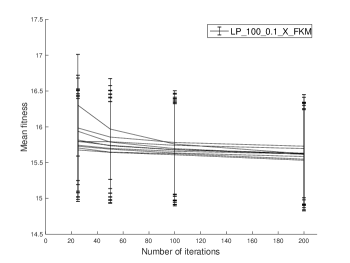
Figure 4: Performance of lbest PSO as a function of the number of iterations, $N_{\rm iter}$, to termination. Each curve corresponds to one of the benchmark functions at ${\rm SNR}=100$ and shows the mean fitness value as a function of $N_{\rm iter}$. The mean fitness value is an average over $N_{R}=1000$ data realizations of the fitness value corresponding to the best model (i.e., $F(M_{\rm best},r_{M_{\rm best}})$ defined in Fig. 2). The error bars represent $\pm 1\sigma$ deviations where $\sigma$ is the sample standard deviation. The other algorithm settings used for this plot can be read off from the key string shown in the legend using Table 2.

VII.1 Sample estimates

In Fig. 5, we show function estimates obtained with SHAPES for arbitrary single data realizations. While not statistically rigorous, this allows an initial assessment of performance when the ${\rm SNR}$ is sufficiently high. Also shown with each estimate is the location of the knots found by SHAPES.

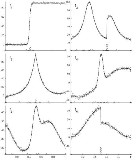
Figure 5: Sample estimated functions for the benchmark functions $f_{1}$ to $f_{6}$. In each panel: the solid black curve is the estimated function; triangles show the locations of its knots (vertically stacked triangles denote repeated knots); the dashed black curve is the true function; gray dots represent the data realization. (In most cases, the solid and dashed curves are visually indistinguishable.) The ${\rm SNR}$s (rounded to integer values) of the functions in order from $f_{1}$ to $f_{6}$ are $1104$, $747$, $506$, $241$, $633$, and $254$, respectively. The algorithm settings were ${\rm LP}\_{\rm SNR}\_0\_100\_{\rm FKM}$ (c.f., Table 2). Note that under these settings, the end B-splines are retained, which requires end knots to have the maximum allowed multiplicity. But this is a fixed multiplicity in each plot and not shown for clarity.

For ease of comparison, we have picked only the benchmark functions ($f_{1}$ to $f_{6}$) used in galvez2011efficient . The SNR of each function matches the value one would obtain using the noise standard deviation tabulated in galvez2011efficient . Finally, the algorithm settings were brought as close as possible by (a) setting the regulator gain $\lambda=0$, (b) using the plain map (c.f., Sec. IV.3), (c) keeping the end knots fixed, and (d) allowing knots to merge. Differences remain in the PSO variant (and associated parameters) used and, possibly, the criterion used for merging knots.

We find that SHAPES has excellent performance at high ${\rm SNR}$ values: without any change in settings, it can fit benchmark functions ranging from spatially inhomogenous but smooth to ones that have discontinuities. For the latter, SHAPES allows knots to coalesce into repeated knots in order to improve the fit at the location of the discontinuities. The sample estimates in Fig. 5 are visually indistinguishable from the ones given in galvez2011efficient . The same holds for the sample estimates given in YOSHIMOTO2003751 , which uses benchmark functions $f_{1}$ to $f_{3}$ and SNRs similar to galvez2011efficient .

VII.2 Regulator gain

While the aim of restricting the number of knots in regression spline is to promote a smoother estimate, it is an implicit regularization that does not guarantee smoothness. In the absence of an explicit regularization, a fitting method based on free knot placement will exploit this loophole to form spurious clusters of knots that fit outliers arising from noise and overfit the data. This issue becomes increasingly important as the level of noise in the data increases.

Fig. 6 illustrates how adding the penalized spline regulator helps mitigate this problem of knot clustering. Shown in the figure is one data realization and the corresponding estimates obtained with high and low values of the regulator gain $\lambda$. For the latter, sharp spikes appear in the estimate where the function value is not high but the noise values are. The method tries to fit out these values by putting more knots in the model and clustering them to form the spikes. Since knot clustering also needs large B-spline coefficients in order to build a spike, a larger penalty on the coefficients suppresses spurious spikes.

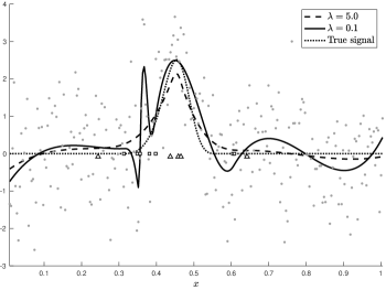
Figure 6: Effect of regulator gain, $\lambda$, on estimation. The solid and dashed curves are the estimates obtained with $\lambda=0.1$ and $\lambda=5.0$ respectively, where $\lambda$ is the regulator gain for the penalty term in Eq. 15. The true curve – benchmark function $f_{7}$ with ${\rm SNR}=10$ – is shown with a dotted line and the gray dots show the data realization. The interior knots in the best model for $\lambda=0.1$ and $\lambda=5.0$ are shown as squares and triangles respectively. (Not shown here is an extra repeated knot for $\lambda=0.1$.) Besides the difference in $\lambda$, the algorithm settings – ${\rm LP}\_10\_\lambda\_50\_{\rm FKM}$ (see Table 2) – were identical for the two estimated curves.

Fig. 7 and Fig. 8 present a statistically more rigorous study of the effect of $\lambda$ by examining the RMSE attained across the whole set of benchmark functions at different ${\rm SNR}$ values. In both figures, the RMSE is shown for identical algorithm settings except for $\lambda$, and in both we observe that increasing the regulator gain improves the RMSE. (The lone case where this is not true is addressed in more detail in Sec. VII.4.) The improvement becomes more pronounced as ${\rm SNR}$ is lowered. (The effect of $\lambda$ on the number of knots in the best fit model at either ${\rm SNR}$ is within the sampling error of the simulation.)

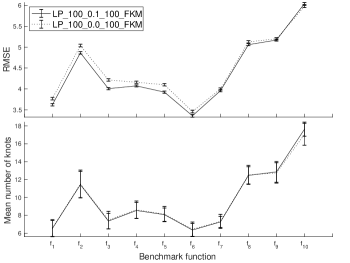
Figure 7: Effect of regulator gain on (top panel) the root mean squared error (RMSE), and (bottom panel) the mean number of knots in the best model for ${\rm SNR}=100$ benchmark functions. In both panels, the solid and dotted curves correspond to $\lambda=0.1$ and $\lambda=0.0$ respectively. The other algorithm settings used for this plot can be read off from the key strings shown in the legend using Table 2. The data points correspond to the benchmark functions shown on the abscissa. The error bars show $\pm 1\sigma$ deviations, where $\sigma$ is the estimated standard deviation.

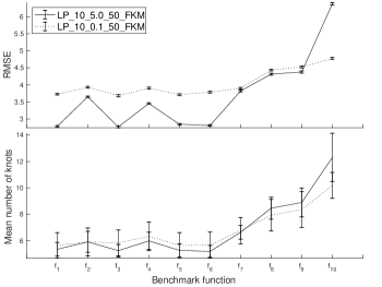
Figure 8: Effect of regulator gain on (top panel) the root mean squared error (RMSE), and (bottom panel) the mean number of knots in the best model for ${\rm SNR}=10$ benchmark functions. In both panels, the solid and dotted curves correspond to $\lambda=5.0$ and $\lambda=0.1$ respectively. The other algorithm settings used for this plot can be read off from the key strings shown in the legend using Table 2. The data points correspond to the benchmark functions shown on the abscissa. The error bars show $\pm 1\sigma$ deviations, where $\sigma$ is the estimated standard deviation.

The higher values of the regulator gains in Fig. 7 and Fig. 8 – $\lambda=0.1$ and $\lambda=5.0$ for ${\rm SNR}=100$ and ${\rm SNR}=10$ respectively – were chosen according to the ${\rm SNR}$. These pairings were chosen empirically keeping in mind that there is an optimum regulator gain for a given noise level. Too high a gain becomes counterproductive as it simply shrinks the estimate towards zero. Too low a value, as we have seen, brings forth the issue of knot clustering and spike formation. Since the latter is a more serious issue for a higher noise level, the optimum regulator gain shifts towards a correspondingly higher value.

VII.3 Results for ${\rm SNR}=100$

We have already selected some of the algorithm settings in the preceding sections, namely, the number of iterations to use and the regulator gain for a given ${\rm SNR}$. Before proceeding further, we need to decide on the remaining ones.

For the ${\rm SNR}=100$ case, it is clear that the end knots and end B-splines must be retained because benchmark functions $f_{1}$ to $f_{6}$ do not all decay to zero and the noise level is not high enough to mask this behavior. Similarly, knot merging is an obvious choice because discontinuities in some of the benchmark functions are obvious at this ${\rm SNR}$ and they cannot be modeled under the alternative option of healing. The remaining choice is between the two knot maps: plain or centered-monotonic.

As shown in Fig. 9, the RMSE is distinctly worsened by the centered-monotonic map across all the benchmark functions. This map also leads to a higher number of knots in the best fit model although the difference is not as significant statistically. Thus, the clear winner here is the map in which knots are merged.

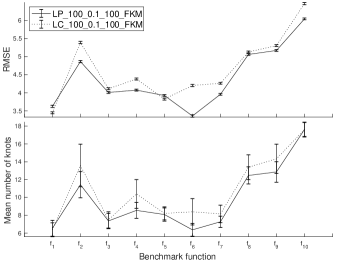
Figure 9: Effect of the map used for transforming PSO search space coordinates to knots on (top panel) the root mean squared error (RMSE), and (bottom panel) the mean number of knots in the best model for ${\rm SNR}=100$ benchmark functions. The solid and dotted curves correspond to the plain and centered-monotonic maps respectively. The other algorithm settings used for this plot can be read off from the key strings shown in the legend using Table 2. The data points correspond to the benchmark functions shown on the abscissa. The error bars show $\pm 1\sigma$ deviations, where $\sigma$ is the estimated standard deviation.

With all the design choices fixed, the performance of SHAPES can be examined. This is done in Fig. 10 and Fig. 11 where the point-wise sample mean and $\pm 2\sigma$ deviation, $\sigma$ being the sample standard deviation, are shown for all the benchmark functions. Note that the level of noise now is much higher than the examples studied in Sec. VII.1.

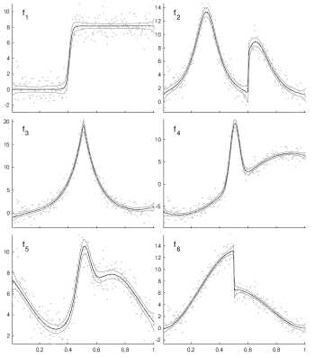
Figure 10: Mean estimated functions (black curve) for benchmark functions $f_{1}$ to $f_{6}$ at ${\rm SNR}=100$. The true functions are shown as dotted curves but they are practically indistinguishable from the mean estimated functions. The gray curves show $\pm 2\sigma$ deviation from the mean function, where $\sigma$ is the estimated standard deviation. The gray dots show an arbitrary data realization for the purpose of visualizing the noise level. The abscissa has the same range for each panel. The algorithm settings used are given by the key string ${\rm LP}\_100\_0.1\_100\_{\rm FKM}$, which can be expanded using Table 2.

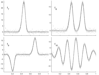
Figure 11: Mean estimated functions (black curve) for benchmark functions $f_{7}$ to $f_{10}$ at ${\rm SNR}=100$. The true functions are shown as dotted curves but they are practically indistinguishable from the mean estimated functions. The gray curves show $\pm 2\sigma$ deviation from the mean function, where $\sigma$ is the estimated standard deviation. The gray dots show an arbitrary data realization for the purpose of visualizing the noise level. The abscissa has the same range for each panel. The algorithm settings used are given by the key string ${\rm LP}\_100\_0.1\_100\_{\rm FKM}$, which can be expanded using Table 2.

It is evident from these figures that SHAPES is able to resolve different types of discontinuities as well as the locations of features such as peaks and sharp changes. In interpreting the error envelope, it should be noted that the errors at different points are strongly correlated, a fact not reflected in the point-wise standard deviation. Thus, a typical single estimate is not an irregular curve bounded by the error envelopes, as would be the case for statistically independent point-wise errors, but a smooth function. Nonetheless, the error envelopes serve to indicate the extent to which an estimate can deviate from the true function.

VII.4 Results for ${\rm SNR}=10$

Here, we examine the case of high noise level at ${\rm SNR}=10$. Fig. 12 and Fig. 13 show the point-wise sample mean and $\pm 2\sigma$ deviation, $\sigma$ being the sample standard deviation, for all the benchmark functions. The algorithm settings used are the same as in Sec. VII.3 for the ${\rm SNR}=100$ case except for the regulator gain and the number of PSO iterations: $\lambda=5.0$ and $N_{\rm iter}=50$ respectively.

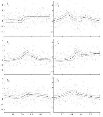
Figure 12: Mean estimated functions (black curve) for benchmark functions $f_{1}$ to $f_{6}$ at ${\rm SNR}=10$. The true functions are shown as dotted curves. The gray curves show $\pm 2\sigma$ deviation from the mean function, where $\sigma$ is the estimated standard deviation. The gray dots show an arbitrary data realization for the purpose of visualizing the noise level. The abscissa has the same range for each panel. The algorithm settings used are given by the key string ${\rm LP}\_10\_5\_50\_{\rm FKM}$, which can be expanded using Table 2.

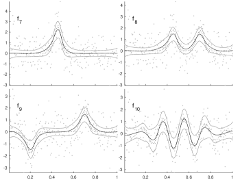
Figure 13: Mean estimated functions (black curve) for benchmark functions $f_{7}$ to $f_{10}$ at ${\rm SNR}=10$. The true functions are shown as dotted curves. The gray curves show $\pm 2\sigma$ deviation from the mean function, where $\sigma$ is the estimated standard deviation. The gray dots show an arbitrary data realization for the purpose of visualizing the noise level. The abscissa has the same range for each panel. The algorithm settings used are given by the key string ${\rm LP}\_10\_5\_50\_{\rm FKM}$, which can be expanded using Table 2.

Unlike the ${\rm SNR}=100$ case, the high noise level masks many of the features of the functions. For example, the discontinuities and the non-zero end values for $f_{1}$ to $f_{6}$ are washed out. Thus, the algorithm settings to use are not at all as clear cut as before. In fact, the results presented next show that alternative settings can show substantial improvements in some cases.

First, as shown in Fig. 14, the estimation of $f_{10}$ actually improves significantly when the regulator gain is turned down to $\lambda=0.1$. While this is the lone outlier in the general trend between regulator gain and RMSE (c.f., Fig. 8), it points to the importance of choosing the regulator gain adaptively rather than empirically as done in this paper.

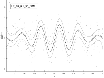
Figure 14: The mean estimated function (black) for benchmark function $f_{10}$ at ${\rm SNR}=10$ with regulator gain $\lambda=0.1$. (The dotted curve shows the true function.) The gray curves show $\pm 2\sigma$ deviation from the mean function, where $\sigma$ is the estimated standard deviation. The gray dots show an arbitrary data realization for the purpose of visualizing the noise level. The other algorithm settings can be read off from the key shown in the plot legend using Table 2.

Next, Fig. 15 examines the effect of the knot map and its interplay with fixing the end knots or allowing them to vary. Allowing the end knots to vary under either knot map leads to a worse RMSE but the number of knots required in the best fit model is reduced, significantly so for $f_{7}$ to $f_{10}$. A plausible explanation for this is that the high noise level masks the behavior of the functions at their end points, and freeing up the end knots allows SHAPES to ignore those regions and focus more on the ones where the function value is higher relative to noise.

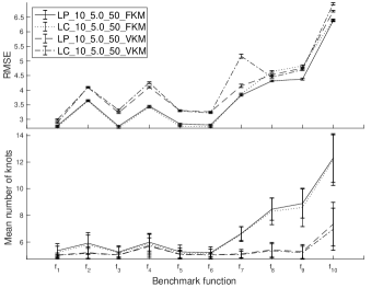
Figure 15: Comparison of plain and centered-monotonic maps under fixed ($F$) and variable ($V$) end knot conditions at ${\rm SNR}=10$. The top and bottom panels respectively show RMSE and mean number of knots in the best model. The other algorithm settings used for this plot can be read off from the key strings shown in the legend using Table 2. The data points correspond to the benchmark functions shown on the abscissa. The error bars show $\pm 1\sigma$ deviations, where $\sigma$ is the estimated standard deviation.

Under a given end knot condition, the centered-monotonic map always performs worse in Fig. 15 albeit the difference is statistically significant for only a small subset of the benchmark functions. Remarkably, this behavior is reversed for some of the benchmark functions when additional changes are made to the design choices. Fig. 16 shows the RMSE when the centered-monotonic map and variable end knots are coupled with the dropping of end B-splines and healing of knots. Now, the performance is better for functions $f_{7}$ to $f_{10}$ relative to the best algorithm settings found from Fig. 15: not only is there a statistically significant improvement in the RMSE for these functions but this is achieved with a substantially smaller number of knots. This improvement comes at the cost, however, of significantly worsening the RMSE for the remaining benchmark functions.

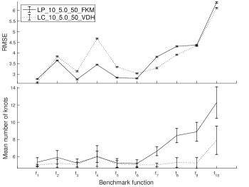
Figure 16: Comparison of plain and centered-monotonic maps under the FKM and VDH algorithm settings respectively at ${\rm SNR}=10$. See Table 2 for the meaning of these and other algorithm settings given by the key strings in the legend. The top and bottom panels respectively show RMSE and mean number of knots in the best model. The data points correspond to the benchmark functions shown on the abscissa. The error bars show $\pm 1\sigma$ deviations, where $\sigma$ is the estimated standard deviation.

VII.5 Effect of bias correction

Fig. 17 shows the effect of using the bias correction step described in Sec. IV.1 on RMSE. We see that bias correction reduces the RMSE for some of the benchmark functions, namely $f_{7}$ to $f_{10}$, and that the reduction is more at higher ${\rm SNR}$ for $f_{10}$. For the remaining benchmark functions, bias correction makes no difference to the RMSE.

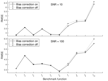
Figure 17: The effect of bias correction on root mean squared error (RMSE) for ${\rm SNR}=10$ (top) and ${\rm SNR}=100$ (bottom) benchmark functions. Solid and dotted curves in each panel correspond to bias correction switched on and off, respectively. The algorithm settings used were ${\rm LP}\_{{\rm SNR}}\_\lambda\_N_{\rm iter}\_{\rm FKM}$ in all the cases with (top) $\lambda=5.0$, $N_{\rm iter}=50$, and (bottom) $\lambda=0.1$, $N_{\rm iter}=100$. These are the fiducial settings used for ${\rm SNR}=10$ and ${\rm SNR}=100$ in Sec. VII.4 and Sec. VII.3, respectively. The data points correspond to the benchmark functions shown on the abscissa. The error bars show $\pm 1\sigma$ deviations, where $\sigma$ is the estimated standard deviation

VII.6 Comparison with other methods

In this section, we compare the performance of SHAPES with WaveShrink donoho1995adapting and smoothing spline reinsch1967smoothing ; craven1978smoothing as implemented in R R-software (called R:sm.spl in this paper). The former is taken from the Matlab-based package WaveLab wavelab and it performs smoothing by thresholding the wavelet coefficients of the given data and applying non-linear shrinkage to threshold-crossing coefficients. For both of these methods, we use default values of their parameters with the following exceptions: for WaveShrink we used the “Hybrid” shrinkage method, while for R:sm.spl we use GCV to determine the regulator gain. For reproducibility, we list the exact commands used to call these methods:

• WaveShrink(Y,‘Hybrid’,L): Y is the data to be smoothed and L is the coarsest resolution level of the discrete wavelet transform of Y.

• smooth.spline(X,Y,cv=FALSE): X is the set of predictor values, Y is the data to be smoothed, and cv=FALSE directs the code to use GCV for regulator gain determination.

Each method above was applied to the same dataset as used for producing Fig. 10. Statistical summaries, namely, the mean estimated function, the $\pm 2\sigma$ deviation from the mean, and RMSE were obtained following the same procedure as described for SHAPES. A crucial detail: when applying WaveShrink, we use $\texttt{L}\in\{1,2,\ldots,6\}$ and pick the one that gives the lowest RMSE.

The results of the comparison are shown in Table 3, Fig. 18, and Fig. 19. Table 3 shows the RMSE values attained by the methods for the benchmark functions $f_{1}$ to $f_{6}$, all normalized to have ${\rm SNR}=100$. Figure 18 shows more details for the benchmark functions that produce the best and worst RMSE values for WaveShrink. Similarly, Fig. 19 corresponds to the best and worst benchmark functions for R:sm.spl.

	SHAPES	WaveShrink	R:sm.spl
$f_{1}$	$3.62$	$7.96$ $(4)$	$4.91$
$f_{2}$	$4.86$	$7.47$ $(4)$	$7.39$
$f_{3}$	$4.01$	$5.82$ $(3)$	$5.52$
$f_{4}$	$4.07$	$8.11$ $(4)$	$5.24$
$f_{5}$	$3.92$	$6.21$ $(3)$	$4.19$
$f_{6}$	$3.36$	$6.93$ $(3)$	$7.62$

Table 3: RMSE values for SHAPES, WaveShrink, and R:sm.spl obtained with the same dataset as used for Fig. 10. The benchmark functions used are $f_{1}$ to $f_{6}$ at ${\rm SNR}=100$. In the case of WaveShrink, the RMSE is the lowest attained over different values of the parameter L. The best value of L is shown parenthetically.

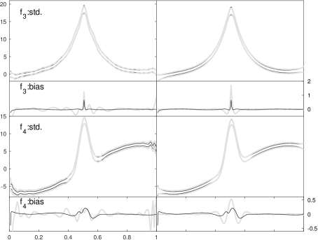
Figure 18: Comparison of SHAPES with alternate methods, WaveShrink and R:sm.spl, for benchmark functions $f_{3}$ and $f_{4}$ at ${\rm SNR}=100$. The left column of figure panels is associated with WaveShrink and the right with R:sm.spl. In each column, (i) the benchmark function used is indicated in each panel, (ii) black curves correspond to SHAPES, and (iii) gray curves to the alternate algorithm. For each benchmark function, there are two panels: (i) The one labeled “std” shows the $\pm 2\sigma$ error envelopes relative to the estimated mean signal from the alternate method; (ii) the one labeled “bias” shows the difference between the true function and the estimated mean signal from each method. The abscissa has the same range for each panel. The ordinate values are identical across the panels in a given row. The dataset used and the algorithm settings for SHAPES are the same as in Fig. 10.

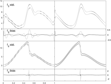
Figure 19: Same as Fig. 18 except for the change in benchmark functions to $f_{5}$ and $f_{6}$.

While noted in the caption of Fig. 18, it is worth re-emphasizing here that the error envelopes of SHAPES shown in Fig. 18 and 19 are computed relative to the mean estimated function of the method being compared to, not to that of SHAPES itself. This modification eliminates visual confusion caused by the different biases (i.e., mean estimated functions) of the methods. However, the bias curves shown separately in these figures do use the respective mean estimated function for each method. The actual mean estimated functions and corresponding error envelopes of SHAPES can be seen in Fig. 10.

From Table 3, we see that SHAPES has the lowest RMSE in all cases. Fig. 18 and Fig. 19 show that this arises from SHAPES generally having both a lower estimation variance (where its error envelope nests within that of the other methods) as well as a lower bias. Typically, R:sm.spl has a lower variance than SHAPES around stationary points of the true function but the difference is marginal. In some cases, such as $f_{3}$ and $f_{6}$, the bias in the SHAPES estimate is significantly lower than that of either WaveShrink or R:sm.spl. In general, WaveShrink estimates are less smooth than those from either SHAPES or R:sm.spl. This is manifested, for example, in the rougher behavior of the mean estimated function from WaveShrink. Both WaveShrink and R:sm.spl have a much poorer resolution of the jump discontinuity in $f_{6}$ compared to SHAPES (c.f., Fig. 10).

VIII Conclusions

Our results show that the challenge of free knot placement in adaptive spline fitting is solvable. The most important element of the solution is the use of an effective metaheuristic for knot optimization. We have shown that lbest PSO is effective in this task. Considering the $f_{10}$ benchmark function for example, the best model found by SHAPES reaches the vicinity of the highest number ($=18$) of non-repeating knots considered in this paper. The good quality of the fit obtained for $f_{10}$ shows that PSO was able to handle this high-dimensional optimization well.

Relative to the SNRs used commonly in the literature on adaptive spline fitting, the values of SNR used in this paper, namely ${\rm SNR}=100$ and ${\rm SNR}=10$, can be ranked respectively as being moderate to low. For the former, discontinuities in function values or derivatives were well localized by SHAPES in all the cases. At the same time, the smooth parts of the benchmark functions were also well estimated. The estimates from SHAPES for low SNR ($=10$) had, naturally, more error. In particular, the noise level in all the data realizations was high enough to completely mask the presence of discontinuities and, thus, they were not well localized. Nonetheless, even with a conservative error envelope of $\pm 2\sigma$ around the mean estimated signal, the overall shape of the true function is visually clear in all the examples. This shows that the estimated functions are responding to the presence of the true function in the data.

While we have characterized the performance of SHAPES as an estimator in this paper, the observation made above for the low ${\rm SNR}$ case suggests that SHAPES may also be used to set up a hypotheses test. This could be based, say, on the fitness value returned by SHAPES. Note that, being a non-parametric method, SHAPES can handle functions with qualitatively disparate behaviors – from a simple change between two levels to oscillatory – without requiring any special tuning. Thus, such a hypotheses test would allow the detection of signals with a wide morphological range. This investigation is in progress.

The dependence of design choices on ${\rm SNR}$, as elucidated in this paper, does not seem to have been fully appreciated in the literature on adaptive spline fitting, probably because the typical scenario considered is that of high ${\rm SNR}$. While performance of SHAPES for ${\rm SNR}=100$ is found to be fairly robust to the design choices made, they have a non-negligible affect at ${\rm SNR}=10$. The nature of the true function also influences the appropriate algorithm settings for the latter case. Fortunately, the settings were found to depend on only some coarse features of a function, such as its behavior at data boundaries ($f_{1}$ to $f_{6}$), whether it is transient ($f_{7}$ to $f_{9}$), or whether it is oscillatory ($f_{10})$. Such features are often well-known in a real-world application domain: it is unusual to deal with signals that have discontinuities as well as signals that are smooth and transient in the same application. Hence, in most such cases, it should be straightforward to pick the best settings for SHAPES.

The inclusion of a penalized spline regulator was critical in SHAPES for mitigating the problem of knot clustering. For all except one ($f_{10}$) benchmark functions considered here, the regulator gain was determined empirically by simply examining a few realizations at each ${\rm SNR}$ with different values of the regulator gain $\lambda$. Ideally, however, $\lambda$ should be determined adaptively from given data using a method such as GCV. The case of $f_{10}$ at ${\rm SNR}=10$ provides a particularly good test bed in this regard: while $\lambda=5.0$ worked well for the other benchmark functions at ${\rm SNR}=10$, the RMSE for $f_{10}$ improved significantly when the gain was lowered to $\lambda=0.1$. Thus, any method for determining $\lambda$ adaptively must be able to handle this extreme variation. We leave the additional refinement of using an adaptive regulator gain in SHAPES to future work.

The extension of SHAPES to multi-dimensional splines and longer data lengths is the next logical step in its development. It is likely that extending SHAPES to these higher complexity problems will require different PSO variants than the one used here.

The codes used in this paper for the FKM option (c.f., Sec. VII.3) are available in a GitHub repository at the URL:
https://github.com/mohanty-sd/SHAPES.git

IX Acknowledgements

The contribution of S.D.M. to this paper was supported by National Science Foundation (NSF) grant PHY-1505861. The contribution of E.F. to this paper was supported by NSF grant PHY-1757830. We acknowledge the Texas Advanced Computing Center (TACC) at The University of Texas at Austin (www.tacc.utexas.edu) for providing HPC resources that have contributed to the research results reported within this paper.

References

- (1) C. de Boor, A Practical Guide to Splines (Applied Mathematical Sciences), Springer, 2001.
- (2) E. J. Wegman, I. W. Wright, Splines in statistics, Journal of the American Statistical Association 78 (382) (1983) 351–365.
- (3) G. Wahba, Spline models for observational data, Vol. 59, Siam, 1990.
- (4) W. Härdle, Applied nonparametric regression, no. 19, Cambridge university press, 1990.
- (5) S. Wold, Spline functions in data analysis, Technometrics 16 (1) (1974) 1–11.
- (6) H. G. Burchard, Splines (with optimal knots) are better, Applicable Analysis 3 (4) (1974) 309–319.
- (7) D. L. Jupp, Approximation to data by splines with free knots, SIAM Journal on Numerical Analysis 15 (2) (1978) 328–343.
- (8) Z. Luo, G. Wahba, Hybrid adaptive splines, Journal of the American Statistical Association 92 (437) (1997) 107–116.
- (9) P. L. Smith, Curve fitting and modeling with splines using statistical variable selection techniques, Tech. rep., NASA, Langley Research Center, Hampton, VA, report NASA,166034 (1982).
- (10) T. Lyche, K. Mørken, A data-reduction strategy for splines with applications to the approximation of functions and data, IMA Journal of Numerical analysis 8 (2) (1988) 185–208.
- (11) J. H. Friedman, B. W. Silverman, Flexible parsimonious smoothing and additive modeling, Technometrics 31 (1) (1989) 3–21.
- (12) J. H. Friedman, Multivariate adaptive regression splines, The Annals of Statistics 19 (1) (1991) 1–67.
- (13) C. J. Stone, M. H. Hansen, C. Kooperberg, Y. K. Truong, et al., Polynomial splines and their tensor products in extended linear modeling: 1994 wald memorial lecture, The Annals of Statistics 25 (4) (1997) 1371–1470.
- (14) G. H. Golub, M. Heath, G. Wahba, Generalized cross-validation as a method for choosing a good ridge parameter, Technometrics 21 (2) (1979) 215–223.
- (15) S. Zhou, X. Shen, Spatially adaptive regression splines and accurate knot selection schemes, Journal of the American Statistical Association 96 (453) (2001) 247–259.
- (16) H. Park, J.-H. Lee, B-spline curve fitting based on adaptive curve refinement using dominant points, Computer-Aided Design 39 (6) (2007) 439–451.
- (17) H. Kang, F. Chen, Y. Li, J. Deng, Z. Yang, Knot calculation for spline fitting via sparse optimization, Computer-Aided Design 58 (2015) 179–188.
- (18) J. Luo, H. Kang, Z. Yang, Knot calculation for spline fitting based on the unimodality property, Computer Aided Geometric Design 73 (2019) 54–69.
- (19) M. Mitchell, An Introduction to Genetic Algorithms by Melanie Mitchell, Bradford, 1998.
- (20) E. Ülker, A. Arslan, Automatic knot adjustment using an artificial immune system for b-spline curve approximation, Information Sciences 179 (10) (2009) 1483–1494.
- (21) P. J. Green, Reversible jump markov chain monte carlo computation and bayesian model determination, Biometrika 82 (4) (1995) 711–732.
- (22) J. Pittman, Adaptive splines and genetic algorithms, Journal of Computational and Graphical Statistics 11 (3) (2002) 615–638.
- (23) I. DiMatteo, C. R. Genovese, R. E. Kass, Bayesian curve-fitting with free-knot splines, Biometrika 88 (4) (2001) 1055–1071.
- (24) F. Yoshimoto, T. Harada, Y. Yoshimoto, Data fitting with a spline using a real-coded genetic algorithm, Computer-Aided Design 35 (8) (2003) 751 – 760.
- (25) S. Miyata, X. Shen, Adaptive free-knot splines, Journal of Computational and Graphical Statistics 12 (1) (2003) 197–213.
- (26) A. Gálvez, A. Iglesias, Efficient particle swarm optimization approach for data fitting with free knot b-splines, Computer-Aided Design 43 (12) (2011) 1683–1692.
- (27) S. D. Mohanty, Particle swarm optimization and regression analysis I, Astronomical Review 7 (2) (2012) 29–35.
- (28) J. Kennedy, R. C. Eberhart, Particle swarm optimization, in: Proceedings of the IEEE International Conference on Neural Networks: Perth, WA, Australia, Vol. 4, IEEE, 1995, p. 1942.
- (29) S. D. Mohanty, Spline based search method for unmodeled transient gravitational wave chirps, Physical Review D 96 (2017) 102008. doi:10.1103/PhysRevD.96.102008.
- (30) S. D. Mohanty, Swarm Intelligence Methods for Statistical Regression, Chapman and Hall/CRC, 2018.
- (31) D. Ruppert, M. P. Wand, R. J. Carroll, Semiparametric regression, Vol. 12, Cambridge University Press, 2003.
- (32) C. H. Reinsch, Smoothing by spline functions, Numerische mathematik 10 (3) (1967) 177–183.
- (33) P. Craven, G. Wahba, Smoothing noisy data with spline functions, Numerische mathematik 31 (4) (1978) 377–403.
-
(34)
R Core Team, R: A Language and Environment
for Statistical Computing, R Foundation for Statistical Computing, Vienna,
Austria (2019).
URL https://www.R-project.org/ - (35) G. Wahba, In discussion Wavelet shrinkage: Asymptopia? with discussion and a reply by Donoho, D. L., Johnstone, I. M., Kerkyacharian, G. and Picard, D., Journal of the Royal Statistical Society Series B 57 (2002) 545–564.
- (36) C. B. Storlie, H. D. Bondell, B. J. Reich, A locally adaptive penalty for estimation of functions with varying roughness, Journal of Computational and Graphical Statistics 19 (3) (2010) 569–589.
- (37) Z. Liu, W. Guo, Data driven adaptive spline smoothing, Statistica Sinica (2010) 1143–1163.
- (38) X. Wang, P. Du, J. Shen, Smoothing splines with varying smoothing parameter, Biometrika 100 (4) (2013) 955–970.
- (39) H. B. Curry, I. J. Schoenberg, On spline distributions and their limits-the polya distribution functions, Bulletin of the American Mathematical Society 53 (11) (1947) 1114–1114.
- (40) M. P. Wand, A comparison of regression spline smoothing procedures, Computational Statistics 15 (4) (2000) 443–462.
- (41) G. Claeskens, T. Krivobokova, J. D. Opsomer, Asymptotic properties of penalized spline estimators, Biometrika 96 (3) (2009) 529–544.
- (42) P. H. Eilers, B. D. Marx, Flexible smoothing with b-splines and penalties, Statistical science (1996) 89–102.
- (43) P. H. Eilers, B. D. Marx, M. Durbán, Twenty years of p-splines, SORT: statistics and operations research transactions 39 (2) (2015) 0149–186.
- (44) D. Ruppert, R. J. Carroll, Theory & methods: Spatially-adaptive penalties for spline fitting, Australian & New Zealand Journal of Statistics 42 (2) (2000) 205–223.
- (45) T. Krivobokova, C. M. Crainiceanu, G. Kauermann, Fast adaptive penalized splines, Journal of Computational and Graphical Statistics 17 (1) (2008) 1–20.
- (46) F. Scheipl, T. Kneib, Locally adaptive bayesian p-splines with a normal-exponential-gamma prior, Computational Statistics & Data Analysis 53 (10) (2009) 3533–3552.
- (47) L. Yang, Y. Hong, Adaptive penalized splines for data smoothing, Computational Statistics & Data Analysis 108 (2017) 70–83.
- (48) T. Krivobokova, Smoothing parameter selection in two frameworks for penalized splines, Journal of the Royal Statistical Society: Series B (Statistical Methodology) 75 (4) (2013) 725–741.
- (49) D. Ruppert, Selecting the number of knots for penalized splines, Journal of computational and graphical statistics 11 (4) (2002) 735–757.
- (50) C. de Boor, On calculating with b-splines, Journal of Approximation Theory 6 (1) (1972) 50 – 62.
- (51) J. Ramsay, B. W. Silverman, Functional data analysis, Springer series in statistics, Springer-Verlag New York, 1997.
- (52) M. J. Lindstrom, Penalized estimation of free-knot splines, Journal of Computational and Graphical Statistics 8 (2) (1999) 333–352.
- (53) V. Goepp, O. Bouaziz, G. Nuel, Spline regression with automatic knot selection, arXiv preprint arXiv:1808.01770.
- (54) H. Akaike, Information theory and an extension of the maximum likelihood principle, in: Selected Papers of Hirotugu Akaike, Springer, 1998, pp. 199–213.
- (55) A. P. Engelbrecht, Fundamentals of computational swarm intelligence, Vol. 1, Wiley Chichester, 2005.
- (56) J. Kennedy, Small worlds and mega-minds: effects of neighborhood topology on particle swarm performance, in: Proceedings of the 1999 Congress on Evolutionary Computation-CEC99 (Cat. No. 99TH8406), Vol. 3, IEEE, 1999, pp. 1931–1938.
- (57) M. E. Normandin, S. D. Mohanty, T. S. Weerathunga, Particle swarm optimization based search for gravitational waves from compact binary coalescences: Performance improvements, Physical Review D 98 (4) (2018) 044029.
- (58) F. J. Solis, R. J.-B. Wets, Minimization by random search techniques, Mathematics of Operations Research 6 (1) (1981) 19–30.
- (59) D. Bratton, J. Kennedy, Defining a standard for particle swarm optimization, in: Swarm Intelligence Symposium, 2007. SIS 2007. IEEE, IEEE, 2007, pp. 120–127.
- (60) C. Leung, Estimation of unmodeled gravitational wave transients with spline regression and particle swarm optimization, SIAM Undergraduate Research Online (SIURO) 8.
- (61) D. Denison, B. Mallick, A. Smith, Automatic bayesian curve fitting, Journal of the Royal Statistical Society: Series B (Statistical Methodology) 60 (2) (1998) 333–350.
- (62) M. Li, Y. Yan, Bayesian adaptive penalized splines, Journal of Academy of Business and Economics 2 (2006) 129–141.
- (63) T. Lee, On algorithms for ordinary least squares regression spline fitting: a comparative study, Journal of statistical computation and simulation 72 (8) (2002) 647–663.
- (64) Matlab Release2018b, The MathWorks, Inc., Natick, Massachusetts, United States.; http://www.mathworks.com/.
- (65) D. L. Donoho, I. M. Johnstone, Adapting to unknown smoothness via wavelet shrinkage, Journal of the american statistical association 90 (432) (1995) 1200–1224.
-
(66)
X. Huo, M. Duncan, O. Levi, J. Buckheit, S. Chen, D. Donoho, I. Johnstone,
About
wavelab.
URL http://statweb.stanford.edu/~wavelab/Wavelab_850/AboutWaveLab.pdf