Quantum critical fluctuations, Planckian dissipation, and compactification scale

Abstract

The most striking result here is that the notion of Planckian dissipation is also applicable to the $c$-axis resistivity of the high temperature cuprate superconductors, and to my knowledge this aspect has not been previously addressed. The derivation involves Kubo formula and does not require any mechanism beyond a non-Fermi liquid assumption. The $c$-axis resistivity, in its essential aspects, is discussed in the context of quantum critical point. Finally, I consider a zero temperature problem with one of its spatial dimensions compactified. The warning is that this compatification scale at the quantum critical point behaves similarly to the finite temperature problem, but obviously being at zero temperature there is no dissipation.

Planckian dissipation has become a widely discussed and important topic Sachdev (2005); Zaanen (2004, 2019), not only from the condensed matter point of view but also from the perspective of high energy physics Hartnoll et al. . Theory also suggests a resolution in the study of quark-gluon plasma formed at heavy ion colliders Policastro et al. (2001). In cuprates, to my knowledge, all such discussion has involved in-plane resistivity. It is quite remarkable that when properly interpreted the notion is also valid for the $c$-axis (perpendicular to the plane) resistivity. The purpose of this paper is to elucidate this aspect and accomplish it by examining the notion of Planckian dissipation and its connection to quantum criticality Chakravarty et al. (1988, 1989).

Consider the conductivity sum rule Kubo (1957) applied to cuprate superconductors. The sum rule applies independently to $ab$-plane and to $c$-direction, perpendicular to the CuO-planes. The $ab$-plane conductivity was invoked previously Hirsch (1992); here we consider the $c$-axis sum rule Chakravarty et al. (1999) which is simpler to apply by comparison. One need not solve a strongly interacting correlated electron problem. Consider the full hamiltonian $H=H_{\rm rest}+H_{c}$; the $c$-axis kinetic energy is defined by

$$H_{c}=-\sum_{ij,s}t_{\perp}(ij,l)c^{\dagger}_{il,s}c_{jl+1,s}+{\rm h.c.}$$ (1)

The remainder, $H_{\rm rest}$, contains no further inter-plane interaction terms, but it is otherwise arbitrary and may contain impurity interactions that couple to the charge density. The hopping matrix element $t_{\perp}(ij,l)$, where $(i,j)$ refers to the sites of the two-dimensional lattice, and $l$ to the layer index. The hopping matrix element can be random in the presence of impurities . The electron operators $(c,c^{\dagger})$ are also labeled by a spin index $s$. We denote the magnitude of $t_{\perp}(ij,l)$ by $t_{\perp}$. One can adapt a sum rule derived first by Kubo Kubo (1957) to get a sum rule for the $c$-axis optical conductivity $\sigma^{c}(\omega,T)$, which is

$$\int_{0}^{\omega_{c}}d\omega\ {\rm Re}\ \sigma^{c}(\omega,T)={\frac{\pi e^{2}d^{2}}{2\hbar^{2}(Ad)}}\langle-H_{c}\rangle.$$ (2)

Here the average refers to the quantum statistical average, $A$ to the two-dimensional area, and $d$ to the separation between the CuO-planes of the unit cells. The hamiltonian $H_{c}$ is an effective hamiltonian valid only for low energy processes, $\omega<\omega_{c}$ that do not involve inter-band transitions, and cannot exceed of order $2-3$ eV.

Since $H_{c}$ is a low-energy effective hamiltonian, the upper limit in Eq. (2) cannot exceed an inter-band cutoff $\omega_{c}$, of order of a few electron volts. Beyond this we need not be more specific, because our goal is to deduce results as $T\to 0$.

To estimate the right hand side, one must make a distinction between Fermi and non-Fermi liquids. While there is no universal theory of non-Fermi liquids, its characterization in terms of spectral function is very useful.We would like to build a model in which the non-Fermi liquid behavior is essential, which we briefly recall: the analytic continuation of the Green’s function to the second Riemann sheet contains branch points instead of simple poles. A spectral function $A$ that satisfies the scaling relation

$$A(\Lambda^{y_{1}}[k-k_{F}],\Lambda^{y_{2}}\omega)=\Lambda^{y_{A}}A([k-k_{F}],\omega),$$ (3)

where $y_{1}$, $y_{2}$, and $y_{A}$ are the exponents defining the universality class of the critical Fermi system. The values of the exponents other than the set $y_{1}=1$, $y_{2}=1$, and $y_{A}=-1$ represent a non-Fermi liquid.

For a non-Fermi liquid, an electron creation operator of wavevector k and spin $\uparrow$ acting on the ground state creates a linear superposition of states that carry the momentum $\bf k$ and spin $\uparrow$. However, the act of inserting an electron into a non-Fermi liquid cannot be renormalized away by defining a single quasiparticle: but the excitation energy is not uniquely related to $\bf k$. The orthogonality catastrophe generally leads to ground state overlaps of the form

$$\langle N|c_{{\bf k}\sigma}|N+1\rangle\approx e^{-\alpha\int_{\omega_{0}({\bf k})}^{\omega_{c}}{d\omega\over\omega}}=\left({\omega_{0}({\bf k})\over\omega_{c}}\right)^{\alpha}.$$ (4)

The quantity $\omega_{0}$ is a low energy cutoff and $\alpha$ is an orthogonality exponent that will depend on electron-electron interactions. Clearly the overlap vanishes as $\omega_{0}\to 0$. The above expression is simply the $z$-factor which must vanish at the Fermi surface in a non-Fermi liquid state. In the superconducting state, the states far above the gap are similar to a non-Fermi liquid normal state. However, in the regions of the Brillouin zone where there is a gap, the orthogonality catastrophe will be cut off because $\omega_{0}$ in Eq. (4) will be of the order of the energy gap $\Delta$, and the overlap factor will be $({\Delta\over\omega_{c}})^{\alpha}$. In the regions where the gap is vanishingly small, orthogonality catastrophe will act with full force.

Thus, the average $\langle H_{c}\rangle$ in the exact ground state $|\widehat{0}\rangle$ to lowest order in $t_{\perp}^{2}/W$ in a perturbative expansion is

$$\langle\widehat{0}|H_{c}|\widehat{0}\rangle=-2\sum_{n\neq 0}\frac{|\langle 0|H_{c}|n\rangle|^{2}}{E_{n}-E_{0}}+\cdots,$$ (5)

where $E_{n}$ and $|n\rangle$ on the right are the eigenvalues and the eigenstates of $H_{\rm rest}$. The first order term is zero, because of the absence of diagonal coherent single particle tunneling between the unit cells, which is due to non-fermi liquid nature of the in-plane excitations.

For conserved parallel momentum, the expansion on the right hand side of Eq. (5) would lead to vanishing energy denominators invalidating the expansion. In a non-Fermi liquid state, however, the matrix elements should vanish for vanishing energy differences, and the the sum is likely to be skewed to high energies. Thus, the energy denominator can be approximated by $W$, of the order of the bandwidth, and the sum can be collapsed using the completeness condition to $\langle 0|H_{c}^{2}|0\rangle/W$. Referring to Eq. 4 and Eq. 5, the difference between $\int_{0}^{W}d\omega\omega^{2\alpha}/\omega$ and $\int_{0}^{W}d\omega\omega^{2\alpha}/W$ is an unimportant numerical factor that can be absorbed in the definition of $W$. Thus the effective hamiltonian is $-H_{c}^{2}/W$.

On dimensional grounds $c$-axis conductivity is

$$\sigma_{c}(T)=a\left(\frac{e^{2}dt_{\perp}^{2}}{AW\hbar^{2}}\right){\frac{1}{\Omega(T)}},$$ (6)

where $a$ is a numerical constant weakly dependent on the band structure. The inelastic scattering time is proportional to the unknown function $1/\Omega(T)$.

We apply the $c$-axis sum rule at two different temperatures $T_{1}$ and $T_{2}$. Quite generally in the superconducting state, $\sigma^{cs}(\omega,T_{1})=D_{c}(T_{1})\delta(\omega)+\sigma^{cs}_{\rm reg}(\omega,T_{1})$, where $D_{c}(T_{1})$ is the superfluid weight. From Eq. (2), it follows that

$$D_{c}(T_{1}) = \int_{0^{+}}^{\omega_{c}}d\omega\bigg{[}{\rm Re}\ \sigma^{cn}(\omega,T_{2})-{\rm Re}\ \sigma^{cs}_{\rm reg}(\omega,T_{1})\bigg{]}$$ (7)

$$+ {\pi e^{2}d^{2}\over 2Ad\hbar^{2}}\bigg{[}\langle-H_{c}(T_{1})\rangle_{s}-\langle-H_{c}(T_{2})\rangle_{n}\bigg{]}.$$

Here, if $T_{2}<T_{c}$, $\langle-H_{c}(T_{2})\rangle_{n}$ is to be understood as taken in the normal state extrapolated below $T_{c}$, and $\sigma^{cn}$ is the corresponding conductivity. Let $T_{1}=T_{2}=0$ in Eq. (7). From the experiments of Ando et al.Ando, it is seen that the $c$-axis response in the normal state obtained by destroying superconductivity is insulating as $T\to 0$; it follows that $\sigma^{cn}(\omega,T=0)\sim\omega^{2}$, as $\omega\to 0$. The regular part $\sigma^{cs}_{\rm reg}(\omega,T=0)$ is also expected to vanish as a power law . At high frequencies the two conductivities must, however, approach each other. Consequently it is reasonable to hypothesize that the conductivity integral on the right hand side of Eq. (7) is negligibly small. Therefore,

$$D_{c}(0)\equiv{c^{2}\over 8\lambda_{c}^{2}}\approx{\pi e^{2}d^{2}\over 2Ad\hbar^{2}}\bigg{[}\langle-H_{c}\rangle_{s}-\langle-H_{c}\rangle_{n}\bigg{]},$$ (8)

where we assumed local London electrodynamics. In any case, the right hand side should be a lower bound. Then

$$\frac{c^{2}}{8\lambda_{c}^{2}}=\frac{4\pi}{a}\sigma_{c}(T)\Omega(T)\left[u_{s}-u_{n}\right],$$ (9)

where $u_{s,n}$ is $\langle 0|(H_{c}/t_{\perp})^{2}|0\rangle_{s,n}$. The average here is with respect to the ground state of $H_{\rm rest}$. The subscripts $s$ and $n$ refer to the superconducting and the normal ground states. By normal state I mean a state in which superconductivity is destroyed. Presently it can be achieved reasonably well by applying high magnetic field Doiron-Leyraud et al. (2007). Only temperature dependencies are contained in the product $\sigma_{c}(T)\Omega(T)$.

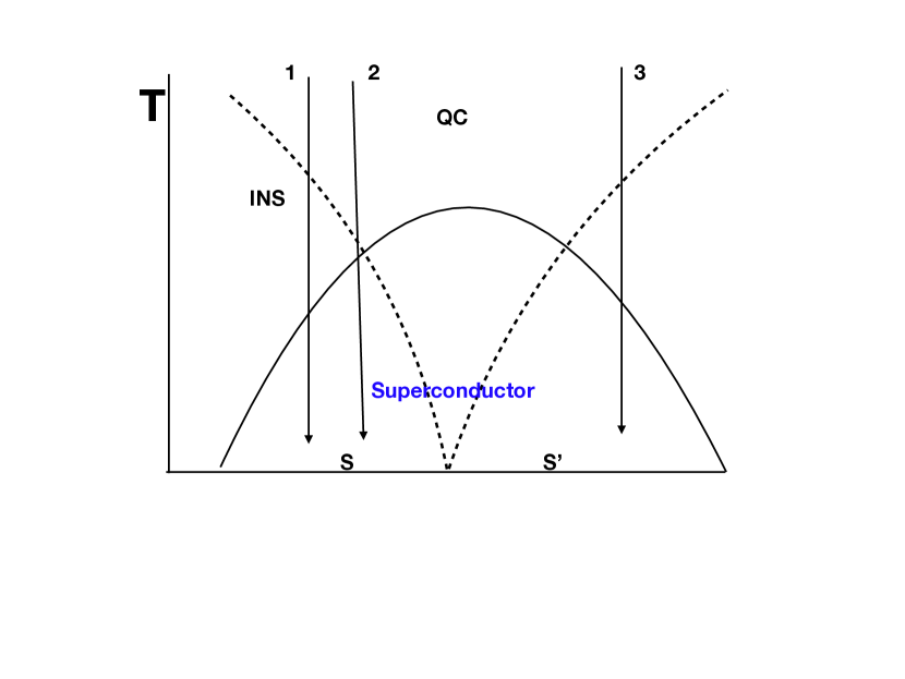
Figure 1: Dimensional crossover of $\rho_{c}$ as a function of temperature $T$. INS stands for insulator and QC for quantum critical. Here S and S’ are two phases, both with superconducting order parameter. For example, S may be $d$-density wave along with superconductivity and S’ without the $d$-density wave. Thus there can be a continuous phase transition. Three vertical arrows are possible experimental trajectories that intersect with quantum critical fan describing a crossover scale Chakravarty et al. (1988, 1989). These trajectories cross over to the superconducting state. There is no reason for the quantum critical point to be in the middle of the superconducting dome as drawn here for simplicity. The line 2 is shown to have very little insulating up turn.

To make progress, we note that the $c$-axis resistivity, $\rho_{c}(T)$, can often be fitted ($p>0$) to a combination of power laws. This power law behavior is not necessary as long as there is a quantum critical crossover. The present form is chosen for convenience:

$$\rho_{c}(T)=b_{1}T^{-p}+b_{2}^{\prime}T.$$ (10)

In some materials such as $\mathrm{YBa_{2}Cu_{3}O_{6+\delta}}$ the $c$-axis resistivity may not be substantially larger from the $ab$-plane resistivity close to $T_{c}$, and may not have a substantial insulating up turn. From the picture, see line 2 in Fig. 1, it is easy to understand to be the case when the the experimental trajectory is very close to the quantum critical line and the superconducting boundary.

We express Eq. (9) in terms of the temperature $T^{*}$ (not the notation for the pseudogap) at which the c-axis resistivity takes its minimum value given the empirical behavior of the $c$-axis resistivity. We get

$$\frac{1}{\lambda_{c}^{2}}=\sigma_{c}(T^{*})T^{*}\left\{\frac{4\pi}{c^{2}}\frac{b_{2}(p+1)}{p}\left[u_{s}-u_{n}\right]\right\},$$ (11)

where $b_{2}=b_{2}^{\prime}(de^{2}t_{\perp}^{2}/\hbar^{2}AW)$. The expression in the curly brackets depends dominantly on $b_{2}$, which describes the high temperature linear resistivity. The low temperature behavior enters only through the exponent $p$, but of course cuts off at $T_{c}$. What could be the meaning of $T^{*}$? At a trivial level it is a lower bound to $\rho_{c}$. I conjecture that it is also the boundary of the quantum critical region above which the linear behavior of the resistivity appears.

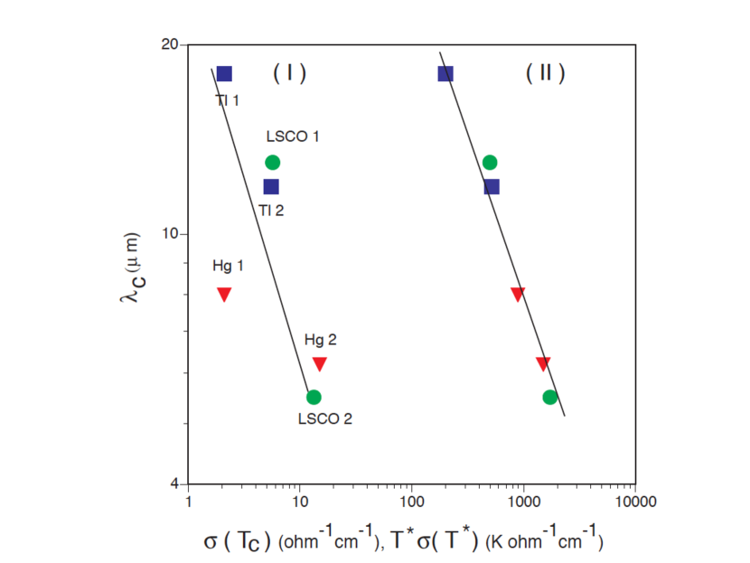
Figure 2: The Basov plot: $\ln\lambda_{c}$ is plotted against $\ln\sigma_{c}(T_{c})$, as in the original Basov plot (I), and against $\ln[T^{*}\sigma_{c}(T^{*})]$ as discussed here (II). The legends in group (II) are the same as those in group (I). Tl1: Ref. Moler et al. (1998) Tl2: Ref. Basov et al. (1999); Hg1: Ref. Kirtley et al. (1998), Hg2: Ref. Basov et al. (1999); LSCO 1 (12%), LSCO 2 (15%): Refs. Loram et al. (1994); Uchida et al. (1996); Nakamura and Uchida (1993).

Thus, provided the expression in curly brackets is a universal constant, a plot of $\ln\lambda_{c}$ against $\ln[\sigma_{c}(T^{*})T^{*}]$ should be a universal straight line, independent of material, and temperature $T^{*}$, which is indeed the case, thus validating Eq. (11). Basov et al.Basov et al. (1994) suggested a similar correlation by plotting $\ln\lambda_{c}$ against $\sigma_{c}(T_{c})$, shown as (I) in Fig. 2 (reproduced from Chakravarty et al. (1999)). In comparison to Basov correlation, the correlation discussed here, shown as (II), is excellent. In Fig. 2, we have taken $T^{*}\approx T_{c}$ for those doped materials that show simply a flattening of $\rho_{c}(T)$ close to $T_{c}$; see the discussion above in reference to Fig. 1. It is at least consistent therefore to assume on dimensional grounds that $\sigma(T^{*})\propto\hbar/k_{B}T^{*}$, indeed a signature of Planckian dissipation. Finally, if $T^{*}$ is any temperature $T$, which lies within the quantum critical fan, a stronger result $\sigma(T)\propto\hbar/k_{B}T$ is plausible. This follows from the fact that the properties in the fan are dictated by the $T=0$ quantum critical point barring crossover scales. From the Basov plot, such a strong plausibility argument is not possible. The extra factor of temperature in the product $\sigma(T)T$, as theoretically predicted, is essential, and was empirically rediscovered by Homes et al Homes et al. (2004) with $T$ replaced arbitrarily by $T_{c}$.

To substantiate the above remark (replacing $T^{*}$ by $T$) note that the correlation length is largely given by the quantum critical fan Chakravarty et al. (1989) within which the physics is largely dictated by the QCP until crossovers take place. A simple one-loop example of crossover is shown below. The full expression for the correlation length in one loop approximation Chakravarty et al. (1989) is,

$$\frac{1}{\xi}=\sqrt{\frac{2}{\pi}}\left(\frac{k_{B}T}{\hbar c}\right)\sinh^{-1}\left(\frac{e}{2}e^{-2\pi\rho_{s}/k_{B}T}\right).$$ (12)

Close to the quantum critical point ($\rho_{s}\to 0$),

$$\frac{1}{\xi}\approx 0.9\left(\frac{k_{B}T}{\hbar c}\right)(1-4.5\rho_{s}/k_{B}T),$$ (13)

Clearly $\xi$ is a result of fluctuations at the quantum critical point. The length scale at the QCP does not reflect a free particle or even a single quasiparticle, but rather a scale invariant description of excitations made explicit by the Euclidean field theory.

Thus, we see that $b_{2}$ in Eq. 11 is indeed inversely proportional to $[u_{s}-u_{n}]$, which is proportional to the $T=0$ superfluid density, $n_{s}^{c}(0)$.The inverse proportionality of $b_{2}$ with $\left[u_{s}-u_{n}\right]$ can be tested in experiments, but has not been thus far.

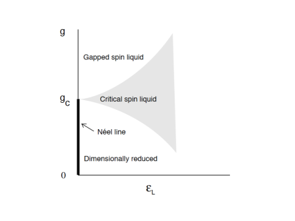
Figure 3: Dimensional crossover at $T=0$ in $d=2$ Here $g$ is a dimensionless coupling constant and $\varepsilon=\frac{\hbar c}{L}$ is an energy-like variable arising from the compactification of $L_{x}$.

We now turn to a simple example Chakravarty (1996) where such a connection to dissipation cannot be made, but in all other respects the problem is similar to the $O(3)$ non-linear $\sigma$-model, where $\hat{\Omega}$ is a three component unit vector, at finite temperature, at least insofar as the quantum critical fan is concerned. Consider a finite $L_{x}$ giving a compactification length, but $\beta\hbar=\infty$. This model has no dissipation but behaves in an analogous manner.

$$\frac{S}{\hbar}=\frac{\rho_{s}^{0}}{2\hbar}\int_{0}^{\beta\hbar}d\tau\int d^{d-1}x\int_{0}^{L}dx_{1}\left[(\partial_{\mu}\hat{\Omega})^{2}+\frac{1}{c^{2}}\left(\frac{\partial\hat{\Omega}}{\partial\tau}\right)^{2}\right],$$ (14)

Lengths in all directions, except $x_{1}$, are infinite; $x_{1}$ is compactified by a periodic boundary condition. The problem at $T=0$ is isomorphic to the problem at finite “temperature”, where the temperature-like variable is $\varepsilon_{L}=\hbar c/L_{x}$, with the identifications of the dimensionless parameters, $g_{0}=\frac{\hbar c\Lambda^{d-1}}{\rho_{s}^{0}}$ and $\varepsilon^{0}_{L}=\frac{\hbar c\Lambda^{d-2}}{L_{x}\rho_{s}^{0}}$, where $\Lambda$ is an arbitrary high energy cutoff, the energy like parameter $\varepsilon^{0}_{L}$ plays the role of the dimensionless temperature-like variable. The relevant excitation velocity will remain unspecified.

There is a quantum critical point with scaie invariant quantum fluctuations, but no dissipation is involved in this problem, merely quantum fluctuations at the quantum critical point. In Fig. 3 (reproduced from Chakravarty (1996)), the Néel line is separated from a gapped spin liquid with an intervening region labeled as critical spin liquid. Originally, this model was used to predict a crossover and deduce the spin gaps in spin ladders, which agreed quite remarkably with numerical calculations.

Later the model was extended Syljuåsen et al. (1997) to finite temperatures to deduce successive crossovers in temperatue, which can be analyzed in terms of Planckian dissipation scales that we leave for future investigations. But to repeat, the $T=0$ model has nothing to do with dissipation.

Recall that in order to discuss Planckian dissipation above we had to introduce a sum rule due to Kubo at $T\neq 0$. This sum rule applies independently for any direction. The $c$-axis sum rule has not been discussed much in this context; see, however, Chakravarty et al. (1999). It is notable that I could combine a simple perturbative expansion, thanks to non-Fermi liquid assumption, with some “empirical” results concerning the $c$-axis resistivity, which is physically clearly justified in Fig. 1. Of course an appeal to universality is implicit. I could have used the $ab$-plane sum rule but in that case a perturbative analysis would not have been applicable because of strong interactions. Later we relied on quantum criticality to arrive at the dissipation scale. Is there any interpretation that we can give to the $T=0$ problem above? A rigorous answer does not exist. I finish by emphasizing that the existence of quantum criticality does not always lead to time scales relevant for dissipation, as discussed in the counterexample. Perhaps one can extend much of the theory to the criticality in the overdoped regime of cuprates Kopp et al. (2007), recently confirmed in Refs. Koshi et al. (2018) and Sarkar et al. (2020).

This work was performed at the Aspen Center for Physics, which is supported by National Science Foundation grant PHY-1607611. It was also partially supported by funds from David S. Saxon Presidential Term Chair at the University of California Los Angeles. I thank M. Mulligan. S. Kivelson and S. Raghu for help and Chandra Varma for general comments.

References

- Sachdev (2005) S. Sachdev, Quantum phase transitions (Cambridge University Press, 2005).
- Zaanen (2004) J. Zaanen, Nature 430, 512 (2004).
- Zaanen (2019) J. Zaanen, SciPost Phys. 6, 61 (2019).
- (4) S. A. Hartnoll, A. Lucas, and S. Sachdev, Holographic Quantum Matter (MIT Press, 2018).
- Policastro et al. (2001) G. Policastro, D. T. Son, and A. O. Startinets, Phys. Rev. Lett. 87, 081601 (2001).
- Chakravarty et al. (1988) S. Chakravarty, B. I. Halperin, and D. R. Nelson, Phys. Rev. Lett. 60, 1057 (1988).
- Chakravarty et al. (1989) S. Chakravarty, B. I. Halperin, and D. R. Nelson, Phys. Rev. B 39, 2344 (1989).
- Kubo (1957) R. Kubo, Journal of the Physical Society of Japan 12, 570 (1957).
- Hirsch (1992) J. E. Hirsch, Physica C: Superconductivity 199, 305 (1992).
- Chakravarty et al. (1999) S. Chakravarty, H.-Y. Kee, and E. Abrahams, Phys. Rev. Lett. 82, 2366 (1999).
- Doiron-Leyraud et al. (2007) N. Doiron-Leyraud, C. Proust, D. LeBoeuf, J. Levallois, J.-B. Bonnemaison, R. Liang, D. A. Bonn, W. N. Hardy, and L. Taillefer, Nature 447, 565 (2007).
- Moler et al. (1998) K. A. Moler, J. R. Kirtley, D. G. Hinks, T. W. Li, and M. Xu, Science 279, 1193 (1998).
- Basov et al. (1999) D. N. Basov, S. I. Woods, A. S. Katz, E. J. Singley, R. C. Dynes, M. Xu, D. G. Hinks, C. C. Homes, and M. Strongin, Science 283, 49 (1999).
- Kirtley et al. (1998) J. R. Kirtley, K. A. Moler, G. Villard, and A. Maignan, Phys. Rev. Lett. 81, 2140 (1998).
- Loram et al. (1994) J. Loram, K. Mirza, J. Wade, J. Cooper, and W. Liang, Physica C: Superconductivity 235-240, 134 (1994).
- Uchida et al. (1996) S. Uchida, K. Tamasaku, and S. Tajima, Phys. Rev. B 53, 14558 (1996).
- Nakamura and Uchida (1993) Y. Nakamura and S. Uchida, Phys. Rev. B 47, 8369 (1993).
- Basov et al. (1994) D. N. Basov, T. Timusk, B. Dabrowski, and J. D. Jorgensen, Phys. Rev. B 50, 3511 (1994).
- Homes et al. (2004) C. C. Homes, S. V. Dordevic, M. Strongin, D. A. Bonn, R. Liang, W. N. Hardy, S. Komiya, Y. Ando, G. Yu, N. Kaneko, X. Zhao, M. Greven, D. N. Basov, and T. Timusk, Nature 430, 539 (2004).
- Chakravarty (1996) S. Chakravarty, Phys. Rev. Lett. 77, 4446 (1996).
- Syljuåsen et al. (1997) O. F. Syljuåsen, S. Chakravarty, and M. Greven, Phys. Rev. Lett. 78, 4115 (1997).
- Kopp et al. (2007) A. Kopp, A. Ghosal, and S. Chakravarty, Proc. National Acad. Sciences, USA 104, 6123 (2007).
- Koshi et al. (2018) K. Koshi, A. Tadashi, M. S. Kensuke, F. Yasushi, K. Takayuki, N. Takashi, M. Hitoshi, Isao.W., M. Masanori, K. Akihiro, K. Ryosuke, and Y. Koike, Phys. Rev. Lett, 121, 057002 (2018).
- Sarkar et al. (2020) T. Sarkar, D. S. Wei, J. Zhang, N. R. Poniatowski, P. R. Mandal, A. Kapitulnik, and R. L. Greene, Science 368, 532 (2020).