Linear-$T$ resistivity from low to high temperature: axion-dilaton theories

Abstract

The linear-$T$ resistivity is one of the hallmarks of various strange metals regardless of their microscopic details. Towards understanding this universal property, the holographic method or gauge/gravity duality has made much progress. Most holographic models have focused on the low temperature limit, where the linear-$T$ resistivity has been explained by the infrared geometry. We extend this analysis to high temperature and identify the conditions for a robust linear-$T$ resistivity up to high temperature. This extension is important because, in experiment, the linear-$T$ resistivity is observed in a large range of temperatures, up to room temperature. In the axion-dilaton theories we find that, to have a robust linear-$T$ resistivity, the strong momentum relaxation is a necessary condition, which agrees with the previous result for the Guber-Rocha model. However, it is not sufficient in the sense that, among large range of parameters giving a linear-$T$ resistivity in low temperature limit, only very limited parameters can support the linear-$T$ resistivity up to high temperature even in strong momentum relaxation. We also show that the incoherent term in the general holographic conductivity formula or the coupling between the dilaton and Maxwell term is responsible for a robust linear-$T$ resistivity up to high temperature.

1 Introduction

It has been shown that strongly correlated electron systems may have interesting universalities regardless of microscopic details. For example, the resistivity ($\rho$) is linear in temperature ($T$) Hartnoll:2016apf

$$\rho\sim T\,,$$ (1)

in various strange metals such as cuprates, heavy fermions and pnictides with a remarkable degree of universality. This is a distinctive property compared with the ordinary metal case, in which $\rho\sim T^{2}$, a different universal property explained by the Fermi liquid theory.

However, this well known “linear-$T$ resistivity” puzzle has not been completely resolved because of the theoretical difficulty in dealing with strong correlation. As a novel and effective tool to address strong correlation in general, the holographic methods or gauge/gravity duality Zaanen:2015oix ; Ammon:2015wua ; Hartnoll:2016apf has been widely used. The basic idea is to understand strongly correlated systems by mapping them to the dual classical gravity systems.

There have been many researches to understand the linear-$T$ resistivity by holographic methods. Most researches, for example Charmousis:2010zz ; Davison:2013txa ; Gouteraux:2014hca ; Kim:2015wba ; Zhou:2015dha ; Ge:2016lyn ; Cremonini:2016avj ; Chen:2017gsl ; Blauvelt:2017koq ; Ahn:2017kvc ; Salvio:2013jia ; Donos:2014cya ; Kim:2014bza ; Kim:2015sma , have focused on the relation between the linear-$T$ resistivity and the infrared (IR) geometry, which can be supported by matter fields and couplings. The IR geometry is characterized by three critical exponent: the dynamical critical exponent ($z$), hyperscaling violating exponent ($\theta$) and charge anomalous parameter ($\zeta$). In particular, Goutéraux Gouteraux:2014hca , for the first time, systematically studied these geometries with momentum relaxation and characterized their scalings in terms of $z,\theta$ and $\zeta$ as well as derived the temperature scaling of the resistivity

$$\rho\sim T^{x(z,\theta,\zeta)}\,,$$ (2)

in low temperature limit. Here, $x$ is some function of critical exponents. It is an interesting result since it gives an understanding of the linear-$T$ resistivity based on the scaling properties of condensed matter systems, which are nicely geometrized in dual gravity models.

However, at the same time, it has an important limitation. The result (2) is valid only in low temperature limit in the sense that $T$ has to be very low compared with any other scales in given models. For example, with a chemical potential ($\mu$) and momentum relaxation (of which strength is denoted by $k$), $T/\mu\ll 1$ and $T/k\ll 1$ etc. Indeed, such a condition enables us to compute the power $x(z,\theta,\zeta)$ analytically. However, noting that the linear-$T$ resistivity has been observed in a ‘large’ range of temperatures, up to room temperature $\sim 300K$ in experiments, the condition of ‘low’ temperature limit for (2) will be too restrictive.

To deal with this problem, we first have to quantify ‘low’ or ‘high’ temperature compared with ‘what’. We may choose the chemical potential $\mu$ as our reference, $T/\mu$. However, it is not clear the relation between ‘$\mu$’ in holography and the chemical potential, $\mu$, in real world. Most holographic models including ours belong to bottom-up models. Without a top-down construction with a precise field theory dual, the meaning of the ‘chemical potential’ (‘$\mu$’) is ambiguous. It is just a ‘chemical potential’ (‘$\mu$’) for ‘some’ conserved $U(1)$ charge. Furthermore, even in the case they are exactly the same quantity, it is still possible that there is some difference in numerical values, for example, $\mu\sim 10`\mu$’ or $\mu\sim 0.01`\mu$’. Thus, for a reference scale, it will be better to choose an intrinsic scale in the model. For example, because experimental results show that the resistivity is linear in $T$ up to $T>T_{c}$ from zero $T$, where $T_{c}$ is the superconducting transition (critical) temperature, $T_{c}$ can play a role as a reference scale. In other words, the ‘low’ or ‘high’ temperature can be defined by the temperature below $T_{c}$ or above $T_{c}$. Of course, it is possible to have a different reference scale other than $T_{c}$ depending on the context. Our purpose here is to motivate why a simple notion of small temperature based on $T/\mu<1$ might be misleading in some cases. For example, in the context of superconductor, $T_{c}$ is a better reference scale than $\mu$ because we have to check if the linear-$T$ resistivity persists up to high temperature $T>T_{c}$. We refer to Jeong:2018tua for more details.

Ref. Jeong:2018tua addressed this issue for the first time, to our knowledge. In this work, the Gubser-Rocha model Gubser:2009qt with momentum relaxation Davison:2013txa ; Zhou:2015qui ; Kim:2017dgz have been considered with a complex scalar field to trigger superconducting instability. It has been shown that these models can exhibit the linear-$T$ resistivity up to ‘high’ temperature, i.e. above $T_{c}$ only if momentum relaxation is strong. The importance of strong momentum relaxation was first emphasized in Hartnoll:2014lpa : it was argued that, if the momentum relaxation, which is extrinsic and non-universal, is strong (quick), transport can be governed by diffusion of energy and charge, which is intrinsic and universal. Thus, the universality of the linear-$T$ resistivity emerges with strong momentum relaxation.

The work in Ref. Jeong:2018tua is important because it is the work studying the linear-$T$ resistivity at ‘high’ temperature, while most of holographic works Davison:2013txa ; Kim:2015wba ; Gouteraux:2014hca ; Zhou:2015dha ; Ge:2016lyn ; Charmousis:2010zz ; Cremonini:2016avj ; Chen:2017gsl ; Blauvelt:2017koq ; Ahn:2017kvc have been focused in the low temperature limit. However, Ref. Jeong:2018tua deals with only one class of models based on the Gubser-Rocha model, so it is not clear if strong momentum relaxation is really necessary and/or sufficient to have the linear-$T$ resistivity in general. The goal of this paper is to investigate this issue in a more general setup.

We start with a most general scaling geometry studied in Davison:2013txa ; Gouteraux:2014hca ; Zhou:2015dha ; Ge:2016lyn ; Cremonini:2016avj ; Chen:2017gsl ; Blauvelt:2017koq ; Ahn:2017kvc , so called axion-dilaton theories or the Einstein-Maxwell-Dilaton with Axion model (EMD-Axion model). The axion field is introduced to realize the momentum relaxation effect. The dilaton field is introduced with some potentials and couplings charaterized by three parameters $(\alpha,\beta,\gamma)$, in order to support the IR geometry parametrized by three scaling exponents ($z,\theta,\zeta$) as explained above (2), which is rich enough to explore various possibilities. The IR geometry with an emblackening factor is valid only at low temperature limit. For the arbitrary temperature solutions, we need to introduce potentials and couplings supporting asymptotically ultraviolate (UV) AdS geometry Kiritsis:2015oxa ; Ling:2016yxy ; Bhattacharya:2014dea . In general, there are many possibilities for potentials and couplings, and in this paper we consider a minimal (one-parameter) UV completion for potentials without changing couplings. This UV completion was introduced in Ling2017 for the purpose of studying the shear viscosity to entropy ratio and includes the Gubser-Rocha model in Jeong:2018tua as a special case.

In short, our strategy is i) start with the various IR geometry giving the linear-$T$ resistivity such that $x(z,\theta,\zeta)=1$ in (2), which is valid only in low $T$ limit; ii) after UV completing the geometry, obtain the arbitrary finite $T$ dependence of resistivity; iii) change the momentum relaxation parameter to see how it affects the robustness of linear-$T$ resistivity at high temperature. As a result, we have found that, in general, the strong momentum relaxation is still necessary to have a robust linear-$T$ resistivity up to higher temperature, but not sufficient: the parameter range for the robust linear-$T$ resistivity is quite limited compared with the high possibility in the low temperature limit Gouteraux:2014hca ; Kim:2015wba ; Zhou:2015dha ; Charmousis:2010zz ; Davison:2013txa ; Ge:2016lyn ; Cremonini:2016avj . We have identified this parameter range which is different from the Gubser-Rocha model. In addition, we have also clarified the term which is responsible for the linear-$T$ resistivity in axion-dilaton theories: it is the incoherent term the first term in the conductivity formula (35) or the coupling between the Maxwell and dilaton fields (for spatial dimension 2).

We organize the paper as follows : In section 2, we review axion-dilaton theories and its low $T$ limit properties focusing on the linear-$T$ resistivity. In section 3, we classify all possible parameter range in the action to obtain the linear-$T$ resistivity in IR and explain our UV-completion. In section 4, we report our results showing a robust linear-$T$ resistivity up to high temperature and demonstrate the importance of strong momentum relaxation. In section 5, we interpret our results in more detail. We identify the term responsible for the linear-$T$ resistivity. We also describe the effects of the parameters introduced in axion-dilaton theories on the temperature dependence of the resistivity. In section 6 we conclude.

2 Axion-dilaton theories: a quick review

In this section, we make a very brief review on the axion-dilaton theory investigated in Gouteraux:2014hca . The purpose of this section is to set the stage and collect the results that will be useful for our discussion later. We refer to the original work Gouteraux:2014hca or a review in Ahn:2017kvc for more detailed explanation and derivations.

2.1 Action and equations of motion

An action of generic EMD-Axion models (or axion-dilaton theories) can be expressed as follows,

$$S=\int\mathrm{d}t\mathrm{d}^{d}x\mathrm{d}r\sqrt{-g}\left(R+\mathcal{L}_{m}\right)\,,$$

$$\mathcal{L}_{m}=\displaystyle-\frac{1}{2}(\partial\phi)^{2}-\frac{J(\phi)}{2}\sum_{i=1}^{d}(\partial\chi_{i})^{2}+V(\phi)-\frac{Z(\phi)}{4}F^{2}\,,$$ (3)

where $\phi$ and $\chi_{i}$ are scalar fields which are called dilaton and axion respectively. The terms denoted by $J$, $Z$, and $V$ are the coupling functions and potential function.

The action yields the following Einstein equations:

$$\begin{split}R_{\mu\nu}&=T_{\mu\nu}-\frac{1}{d}g_{\mu\nu}T\\ &=\frac{1}{2}\partial_{\mu}\phi\partial_{\nu}\phi+\frac{J(\phi)}{2}\sum_{i=1}^{d}\partial_{\mu}\chi_{i}\partial_{\nu}\chi_{i}+\frac{Z(\phi)}{2}F_{\mu}{{}^{\rho}}F_{\nu\rho}-\frac{Z(\phi)F^{2}}{4d}g_{\mu\nu}-\frac{V(\phi)}{d}g_{\mu\nu}\,,\\ \end{split}$$ (4)

where $T_{\mu\nu}:=-\frac{1}{\sqrt{-g}}\frac{\delta(\sqrt{-g}\mathcal{L}_{m})}{\delta g^{\mu\nu}}$ and $T=g^{\mu\nu}T_{\mu\nu}$  . The Maxwell equation, scalar equation, and axion equation are

$$\begin{split}&\nabla_{\mu}(Z(\phi)F^{\mu\nu})=0\,,\\ &\square\phi+V^{\prime}(\phi)-\frac{1}{4}Z^{\prime}(\phi)F^{2}-\frac{1}{2}J^{\prime}(\phi)\sum_{i=1}^{d}(\partial\chi_{i})^{2}=0\,,\\ &\nabla_{\mu}(J(\phi)\nabla^{\mu}\chi_{i})=0\,.\end{split}$$ (5)

By considering the following homogeneous (meaning all functions are only functions of $r$) ansatz

$$\begin{split}&\mathrm{d}s^{2}=-D(r)\mathrm{d}t^{2}+B(r)\mathrm{d}r^{2}+C(r)\sum_{i=1}^{d}\mathrm{d}x_{i}^{2}\,,\\ &\phi=\phi(r)\,,\quad A=A_{t}(r)\mathrm{d}t\,,\quad\chi_{i}=kx_{i}\,,\end{split}$$ (6)

we obtain the Einstein equations

$$\!0=\frac{Z(d-1)A_{t}^{\prime 2}}{dD}+\frac{2BV}{d}+\frac{B^{\prime}D^{\prime}}{2BD}-\frac{dD^{\prime}C^{\prime}}{2DC}+\frac{D^{\prime 2}}{2D^{2}}-\frac{D^{\prime\prime}}{D}\,,$$ (7)

$$\!0=\phi^{\prime 2}-\frac{dC^{\prime 2}}{2C^{2}}-\frac{dC^{\prime}D^{\prime}}{2CD}-\frac{dC^{\prime}B^{\prime}}{2CB}+\frac{dC^{\prime\prime}}{C}\,,$$ (8)

$$\!0=\frac{Jk^{2}B}{C}-\frac{2BV}{d}+\frac{ZA_{t}^{\prime 2}}{dD}+\frac{C^{\prime}}{2C}\left(\frac{D^{\prime}}{D}-\frac{B^{\prime}}{B}\right)+\frac{(d-2)C^{\prime 2}}{2C^{2}}+\frac{C^{\prime\prime}}{C}\,,$$ (9)

which come from the equations corresponding to $R_{tt},R_{rr}$, and $R_{xx}$ in (4) respectively. The prime ^′ denotes the derivative with respect to $r$. The Maxwell equation and scalar equation are reduced to

$$0=\left[Z\frac{C^{\frac{d}{2}}}{\sqrt{BD}}A_{t}^{\prime}\right]^{\prime}\,,$$ (10)

$$0=-\frac{dJ_{,\phi}k^{2}B}{2C}+\frac{Z_{,\phi}A_{t}^{\prime 2}}{2D}+BV_{,\phi}-\frac{B^{\prime}\phi^{\prime}}{2B}+\left(\frac{dC^{\prime}}{2C}\right)\phi^{\prime}+\frac{D^{\prime}\phi^{\prime}}{2D}+\phi^{\prime\prime}\,,$$ (11)

and the axion equations are satisfied trivially.

2.2 IR analysis of the axion-dilaton theories

Our task is to find the functions $B(r),C(r),D(r),A_{t}(r)$, and $\phi(r)$ in the ansatz (6) satisfying the equations of motion (7)-(11) for a given the couplings and potential functions in $J,Z$ and $V$ in (2.1).

In order to have analytic scaling solutions in IR (Infrared: far from the AdS boundary), we give the following constrains to $J,Z$ and $V$ in IR:

$$V(\phi)\sim V_{0}e^{\alpha\phi}\,,\qquad J(\phi)\sim e^{\beta\phi}\,,\qquad Z(\phi)\sim e^{\gamma\phi}\,,$$ (12)

where the constant parameters ($\alpha,\beta,\gamma,V_{0}$) are introduced. We consider the coefficient $V_{0}$ only for $V$ without loss of generality because the overall factors for $J$ and $Z$ can be absorbed into the field $\chi_{i}$ and $A_{t}$. Plugging the “IR scaling coupling” (12) into the equations of motion (7)-(11) with the following scaling solution ansatz,

$$\begin{split}&\mathrm{d}s^{2}=r^{\frac{2\theta}{d}}\left(-\frac{\mathrm{d}t^{2}}{r^{2z}}+\frac{L^{2}\mathrm{d}r^{2}}{r^{2}}+\frac{\sum_{i=1}^{d}\mathrm{d}x_{i}^{2}}{r^{2}}\right)\,,\\ &A_{t}=Qr^{\zeta-z}\,,\quad\phi=\kappa\ln{(r)}\,,\quad\chi_{i}=kx_{i}\,,\end{split}$$ (13)

we obtain the solution ($z$, $\theta$, $\zeta$, $L$, $Q$, $\kappa$) in terms of $(\alpha,\beta,\gamma,V_{0},k)$. We will call the exponents ($z$, $\theta$, $\zeta$) and the coefficients ($L,Q,\kappa$) “solution parameters” or “output parameters”. We will call the parameters $(\alpha,\beta,\gamma,V_{0},k)$ “action parameters” or “input parameters”. Physically, $Q$ is proportional to the charge density and $k$ means the strength of the momentum relaxation. Note that $\phi\to\pm\infty$ in IR as $r\to\infty$ where $J\sim r^{\kappa\beta},Z\sim r^{\kappa\gamma}$ and $V\sim r^{\kappa\alpha}$.

After plugging scaling solution ansatz (13) into equations of motion (7)$\sim$(11), we find that there are four possibilities to satisfy the equations of motion. We may classify these solutions according to the “relevance” of the axion and/or charge, following Gouteraux:2014hca . By “marginally relevant axion” we mean the axion parameter $k$ appear explicitly in the leading solutions and by “marginally relevant charge” we mean $Q$ appears explicitly in the leading solutions. By “irrelevant axion (charge)” we mean $k$ $(Q)$ do not appear explicitly in the leading solutions but they can appear in the sub-leading solutions. Therefore, we may consider four classes as follows.

• class I: marginally relevant axion $\&$ charge           ($k\neq 0,Q\neq 0$)

• class II: marginally relevant axion $\&$ irrelevant charge     ($k\neq 0,Q=0$)

• class III: irrelevant axion $\&$ marginally relevant charge    ($k=0,Q\neq 0$)

• class IV: irrelevant axion $\&$ charge              ($k=0,Q=0$)

Notice that the classification is based on the property of the leading solutions. To have a more complete picture, we also should consider the deformation by the sub-leading solutions:

$$\Phi_{i}\rightarrow\Phi_{i}+\epsilon_{i}r^{\beta_{i}}+\cdots\,,$$ (14)

where $\Phi_{i}$ denotes every leading order solution collectively, $\epsilon_{i}$ is a small parameter and $\beta_{i}$ denotes the exponent of the sub-leading order and $\beta_{i}<0$ $(\beta_{i}>0)$ when the IR is located at $r\rightarrow\infty$ $(r\rightarrow 0)$. Therefore, $Q=0$ in the leading solution does not mean zero density and $k=0$ in the leading solution does not mean no momentum relaxation because these parameters can appear in the sub-leading solutions. In particular, if the axion is relevant, we may expect the momentum relaxation affects IR physics more strongly than the irrelevant axion cases.

We present the explicit solutions for every classes in the following.

Class I: charge and axions are marginally relevant

The leading order solutions read

$$\begin{split}&z=\frac{-2+d\alpha^{2}-d\beta^{2}}{d(\alpha-\beta)\beta}\,,\qquad\theta=\frac{d\alpha}{\beta}\,,\qquad\zeta=\frac{\alpha+\gamma}{\beta}\,,\qquad\kappa=-\frac{2}{\beta}\,,\\ &L^{2}=-\frac{2(d-\theta+z-1)(d-\theta+z)}{(d-1)k^{2}-2V_{0}}\,,\qquad Q^{2}=\frac{2(dz-\theta)k^{2}-4V_{0}(z-1)}{((d-1)k^{2}-2V_{0})(d-\theta+z)}\,,\end{split}$$ (15)

as well as a constraint between input parameters:

$$\gamma=(d-1)\alpha-d\beta\,.$$ (16)

or output parameters:

$$d+\zeta-\theta=0\,.$$ (17)

Class II: charge is irrelevant; axions are marginally relevant

The leading order solutions read

$$\begin{split}&z=\frac{-2+d\alpha^{2}-d\beta^{2}}{d(\alpha-\beta)\beta}\,,\qquad\theta=\frac{d\alpha}{\beta}\,,\qquad\kappa=-\frac{2}{\beta}\,,\\ &L^{2}=\frac{(d-\theta+z)(dz-\theta)}{V_{0}}\,,\end{split}$$ (18)

as well as a constraint between input parameters:

$$k^{2}=\frac{2V_{0}(z-1)}{dz-\theta}\,.$$ (19)

Note that the $Q$ and $\gamma$ does not appear in the solutions (18) and the constrain (19) can be understood as the condition $Q=0$ in (15) so $\zeta$ is also undetermined.

The value of $Q$ and $\zeta$ and their $\gamma$ dependences will be determined in the subleading order

$$\zeta=d-\kappa\gamma-\frac{d-2}{d}\theta=d+\frac{2\gamma}{\beta}-\frac{(d-2)\alpha}{\beta}\,.$$ (20)

As explained in (14), this subleading order solution will back-react to metric and dilaton field, which behave as

$$\sim r^{d+\zeta-\theta}\,.$$ (21)

To have a stable IR geometry, we impose the constraint

$$d+\zeta-\theta<0\,,$$ (22)

near IR, $r\rightarrow\infty$. In terms of $\alpha,\beta,\gamma$ this constraint means

$$2d-\frac{2(d-1)\alpha}{\beta}+\frac{2\gamma}{\beta}<0\,.$$ (23)

Class III: charge is marginally relevant; axions are irrelevant

The leading order solutions read

$$\begin{split}&z=\frac{4d-\kappa^{2}(d\alpha^{2}-2)}{2d(2+\alpha\kappa)}\,,\quad\theta=\frac{d^{2}\alpha}{(d-1)\alpha-\gamma}\,,\quad\zeta=-\frac{1}{2}\kappa(\alpha+\gamma)\,,\quad\kappa=-\frac{2d}{(d-1)\alpha-\gamma}\,,\\ &L^{2}=\frac{(d-\theta+z-1)(d-\theta+z)}{V_{0}}\,,\qquad Q^{2}=\frac{2(z-1)}{d-\theta+z}\,.\end{split}$$ (24)

Note that the $k$ and $\beta$ does not appear in the solutions (24) so, compared with class I and II solutions, $\kappa\beta=-2$ does not hold anymore. The solutions (24) may be understood from (15) by setting $k=0$ and replacing $\beta$ by using (16).

Similarly to class II, in the subleading order, the axion $(\chi_{i}=kx_{i})$ starts playing a role and its back-reaction to metric and dilaton field behaves as

$$\sim r^{2+\kappa\beta}\,.$$ (25)

To have a stable IR, we impose the constraint

$$2+\kappa\beta<0\,,$$ (26)

in the IR, $r\rightarrow\infty$. In terms of $\alpha,\beta,\gamma$ this constraint means

$$2+\frac{2d\beta}{\gamma-(d-1)\alpha}<0\,.$$ (27)

Class IV: charge and axions are irrelevant

The leading order solutions read

$$z=1\,,\qquad\theta=\frac{d^{2}\alpha^{2}}{d\alpha^{2}-2}\,,\qquad\kappa=-\frac{2d\alpha}{d\alpha^{2}-2}\,,\qquad L^{2}=\frac{(d-\theta)(d-\theta+1)}{V_{0}}\,.$$ (28)

Note that the $Q$, $\gamma$, $k$, and $\beta$ do not appear in the solutions. The solutions (28) can be understood from (24) by setting $Q=0$ or $z=1$. Similarly to case II the subleading gauge field yields

$$\zeta=d-\kappa\gamma-\frac{d-2}{d}\theta=\frac{2d(\alpha(\alpha+\gamma)-1)}{d\alpha^{2}-2}\,.\,$$ (29)

Similarly to class II and III we have the following constraints, (21) and (25):

$$d+\zeta-\theta<0\quad\mathrm{and}\quad 2+\kappa\beta<0\,,$$ (30)

or equivalently

$$\frac{2d(\alpha(\alpha+\gamma)-2)}{d\alpha^{2}-2}<0\quad\mathrm{and}\quad 2-\frac{2d\alpha\beta}{d\alpha^{2}-2}<0\,.$$ (31)

2.3 Resistivity in low temperature limit

Furthermore, it turns out that the emblackening factor $f(r)$

$$f(r)=1-\left(\frac{r}{r_{H}}\right)^{z+d-\theta}\,,$$ (32)

can be turned on ($\mathrm{d}t^{2}\rightarrow f\mathrm{d}t^{2}$ and $\mathrm{d}r^{2}\rightarrow\mathrm{d}r^{2}/f$ in (13)) for all classes. Then, the Hawking temperature from this emblackening factor allows us to study the axion-dilaton theories at low temperature. However, it should be emphasized that the solution with this emblackening factor is valid only for very low temperature compared with any other scales, for example, chemical potential and momentum relaxation.

In this low temperature limit, the Hawking temperature $T$ and charge density $q$ can be expressed in terms of solution parameters $(z,\theta,\zeta,Q)$: Gouteraux:2014hca ; Ahn:2017kvc

$$T:=\frac{1}{4\pi}\left.\frac{|D^{\prime}|}{\sqrt{DB}}\right|_{r_{H}}=\frac{|d+z-\theta|}{4\pi}r_{H}^{-z}\,,$$ (33)

$$q:=\left.\sqrt{\frac{C^{d}}{DB}}ZA_{t}^{\prime}\right|_{r_{H}}=Q(\zeta-z)\,,\quad s:=\left.4\pi C^{d/2}\right|_{r_{H}}=4\pi r_{H}^{\theta-d}\,,$$ (34)

where the subscript H denotes horizon. The transport coefficients, for instance electric conductivity or thermal conductivity, can be calculated Gouteraux:2014hca ; Donos:2014cya . Especially the electric DC conductivity formula for the EMD-Axion model is given by

$$\sigma_{DC} =Z_{H}C_{H}^{\frac{d-2}{2}}+\frac{q^{2}}{k^{2}C_{H}^{d/2}J_{H}}$$ (35)

$$\sim T^{-(2-\zeta)/z}+\frac{q^{2}}{k^{2}}T^{-\frac{d-\theta-\kappa\beta}{z}}\,.$$ (36)

Note that only the behavior of ($Z,J,C$) at the horizon play a role in determining the power of $T$ via the relation between $r_{H}$ and $T$ (33). More variables ($A_{t},B,C,D,Z$) enter for the charge density $q$ as shown in (34).

By using the constraints between $\zeta,\beta,\kappa$, (16), (22), (26), (30), we can find which term in (35) is dominant in low temperature limit. In class I both two terms are of the same order, in class II the first term is dominant, in class III the second term is dominant, and in class IV the dominant term depends on the parameters. i.e.  in low temperature limit the resistivity $\rho\sim\sigma_{DC}^{-1}$ behaves as:

$$\begin{split}&\text{Class I \ \ : }\rho\sim T^{(2+d-\theta)/z}\,,\\ &\text{Class II \ : }\rho\sim T^{\frac{2-\zeta}{z}}\,,\\ &\text{Class III : }\rho\sim T^{\frac{d-\theta-\kappa\beta}{z}}\,,\\ &\text{Class IV : }\rho\sim T^{d-\theta-\kappa\beta}\quad\text{or}\,\,\,T^{2-\zeta}\,.\end{split}$$ (37)

Note that the power $x$ in $\rho\sim T^{x}$ does not depend on the momentum relaxation $k$. This is because this formula is valid only in low temperature limit. At finite temperature, this is not the case as we will show.

In fact, in addition to the constrains, (16), (22), (26), (30), there are more constraints for the exponents $z$ and $\theta$, which will be necessary to constrain our physical model later. First, since we are considering the case that IR is located at $r\rightarrow\infty$, the exponent of $r$ of each metric component in (13) should be negative, which implies

$$\theta<dz\,,\quad\theta<d\,.$$ (38)

Second, the emblackness factor (32) $f(r)\rightarrow 1$ at the UV ($r\to 0$), which implies

$$\theta<z+d\,.$$ (39)

Third, the condition that the specific heat is positive implies

$$\frac{d-\theta}{z}>0\,,$$ (40)

where we used the relation between the entropy and temperature (33): $s\sim T^{\frac{(d-\theta)}{z}}$. Fourth, the $\kappa,Q,$ and $L$ in the (15), (18) and (24) should be real. The $\kappa$ can be rewritten by :

$$\kappa^{2}=\frac{2(d-\theta)(d(z-1)-\theta)}{d}\,.$$ (41)

The conditions (38) - (39) and $Q^{2}>0,\,L^{2}>0,\,\kappa^{2}>0$ imply

$$z>1,\quad\theta<d\,.$$ (42)

Note that Eqs. (30) and (42) imply that both $2-\zeta$ and $d-\theta-\kappa\beta$ can not be 1 in class IV. Thus, the class IV solution does not allow the linear-$T$ resistivity in the low temperature limit. Being interested in the linear-$T$ resistivity, we study only class I, II and III solutions in the following section.

3 Resistivity up to high temperature

From (37), we may obtain the condition for the linear-$T$ resistivity. However, as we emphasized in the previous section, the temperature dependence of the resistivity (37) is valid only in low temperature limit, which means that the temperature is very low compared with any other scales such as the chemical potential, the momentum relaxation strength, or the superconducting phase transition scale. However, from experimental results, it is important to have a robust linear-$T$ resistivity also at intermediate and high temperature, which we will call finite temperature to distinguish it from low temperature limit.

3.1 UV-completion of potentials

At finite temperature, the couplings and potential in (12) only valid in IR have to be UV-completed. In order to have asymptotically AdS space in UV, we impose the following conditions Charmousis:2010zz :

$$V(\phi)=\frac{(d+1)d}{\ell_{AdS}^{2}}-\frac{1}{2}m^{2}\phi^{2}+\cdots\,,$$ (43)

$$Z(\phi)=1+\cdots\,,\quad J(\phi)=1+\cdots\,,$$ (44)

near boundary ($r\sim 0$). In other words, for $V(\phi)$,

$$V(0)=-2\Lambda=\frac{(d+1)d}{\ell_{AdS}^{2}}\,,\qquad V^{\prime}(0)=0\,,\qquad V^{\prime\prime}(0)=-m^{2}=\frac{-\Delta(\Delta-d-1)}{\ell_{AdS}^{2}}\,,$$ (45)

where $\Delta$ is the conformal dimension of the dual operator of $\phi$ and $\phi\rightarrow 0$ in UV. For simplicity we set $\ell_{AdS}=1$ from here.

In principle, there will be many possibilities to construct $V,Z,J$ satisfying (12) in IR and (43) and (44) in UV. See for example Gouteraux:2011ce ; Kiritsis:2015oxa ; Ling2017 ; Davison:2018nxm . Here, for simplicity, we choose one minimal way studied in Ling2017 :

$$Z(\phi)=e^{\gamma\phi}\,,\qquad J(\phi)=e^{\beta\phi}\,,$$ (46)

and three cases for $V(\phi)$

$$\begin{split}&V(\phi)=\left\{\begin{array}[]{lll}\frac{2d}{\alpha^{2}}\sinh^{2}\left(\frac{\alpha\phi}{2}\right)+(d+1)d\,,&\text{for}\,\theta<0\,,\\[2.15277pt] (d+1)d\,,&\text{for}\,\theta=0\,,\\[2.15277pt] d\left(\frac{1}{\alpha^{2}}+2\left(d+1\right)\right)\operatorname{sech}(\alpha\phi)-d\left(\frac{1}{\alpha^{2}}+\left(d+1\right)\right)\operatorname{sech}^{2}\left(\alpha\phi\right),&\text{for}\,d>\theta>0\,.\end{array}\right.\end{split}$$ (47)

Let us now explain the rationale for our choice. All $V(\phi)$ in (47) satisfy the expansion (43), where the dilaton mass $m^{2}=-d$ for $\theta\neq 0$ and $m^{2}=0$ for $\theta=0$. The dilaton $\phi$ behaves near boundary as follows

$$\phi(r)\sim\begin{cases}c+\cdots,\quad\theta=0\,,\\ r+\cdots,\quad\theta\neq 0\,,\end{cases}$$ (48)

where $c$ is a constant and we will set $c=0$. Thus, our choice of the dilaton mass makes (46) satisfy the UV condition (44). The particular choice of $V_{0}$ we make is not necessary but for simplicity. Thanks to this choice, our $V(\phi)$ becomes a function of only $\alpha$.

We consider three kinds of $V(\phi)$ depending on the sign of $\theta$ in (47). To understand the necessity of these three different forms let us first find the relation between the signs of $\alpha$ and $\theta$. Near IR $r\rightarrow\infty$, we choose $\phi\rightarrow+\infty$, which means $\kappa>0$ from (13). When $\kappa>0$, the relations between $\alpha$ and $\theta$ in (15), (18), (24) imply that the signs of $\theta$ and $\alpha$ are opposite, and if $\theta=0$ then $\alpha=0$. Thus, we find that the asymptotic potentials near IR read

$$\begin{split}&V(\phi)=\left\{\begin{array}[]{lll}\frac{d}{2\alpha^{2}}\left(e^{\alpha\phi}+e^{-\alpha\phi}-2\right)+(d+1)d\approx V_{0}e^{\alpha\phi}\,,&V_{0}=\frac{d}{2\alpha^{2}}\,,&\text{for}\,\alpha>0\,,\\[2.15277pt] (d+1)d\,,&V_{0}=(d+1)d\,,&\text{for}\,\alpha=0\,,\\[2.15277pt] \frac{d\left(\frac{1}{\alpha^{2}}+2(d+1)\right)}{\cosh\left(\alpha\phi\right)}-\frac{d\left(\frac{1}{\alpha^{2}}+(d+1)\right)}{\cosh^{2}\left(\alpha\phi\right)}\approx V_{0}e^{\alpha\phi}\,,&V_{0}=2d\left(\frac{1}{\alpha^{2}}+2d+2\right),&\text{for}\,\alpha<0\,,\end{array}\right.\end{split}$$ (49)

which precisely match to our IR condition $V\sim V_{0}e^{\alpha\phi}$ in (12). For example, the first potential will take a form of $V_{0}e^{-\alpha\phi}$ for $\alpha<0$, which is not consistent with our IR condition $V\sim V_{0}e^{\alpha\phi}$ in (12).

Note that the first potential in (47) includes the Gubser-Rocha model with linear axion. For $(\alpha,\beta,\gamma)=(1/\sqrt{3},0,-1/\sqrt{3})$ and $d=2$, $V(\phi),Z(\phi)$ and $J(\phi)$ in (46) and (47) yield

$$V(\phi)=6\cosh{\frac{\phi}{\sqrt{3}}}\,,\qquad Z(\phi)=e^{-\frac{\phi}{\sqrt{3}}}\,,\qquad J(\phi)=1\,,$$ (50)

which is nothing but the Gubser-Rocha model with linear axion studied in Gouteraux:2014hca ; Jeong:2018tua .

3.2 Numerical methods

Because the potential is changing, the scaling solution (13) is not valid anymore so we start with the following ansatz :

$$\begin{array}[]{l}\mathrm{d}s^{2}=\displaystyle\frac{1}{u^{2}}\left(-(1-u)U(u)e^{-S(u)}\mathrm{d}t^{2}+\frac{\mathrm{d}u^{2}}{(1-u)U(u)}+\sum_{i=1}^{d}\mathrm{d}x_{i}^{2}\right)\,,\\ \phi=\phi(u)\,,\qquad\chi_{i}=kx_{i}\,,\qquad A=(1-u)A_{t}(u)\mathrm{d}t\,,\end{array}$$ (51)

where $u:=r/r_{h}$. In this coordinate, the horizon and the boundary are located at $u=1$ and $u=0$ respectively. Since we want the geometry to be asymptotically $AdS_{d+2}$ near boundary, we impose the conditions $U(0)=1$ and $S(0)=0$.

In our set-up, there are three dimensionful parameters: the chemical potential $\mu=A_{t}(0)$, the Hawking temperature $T$, and the momentum relaxation strength $k$. For numerical analysis, we will take $d=2$. We choose the chemical potential as our scale so the dimensionless parameters are $T/\mu$ and $k/\mu$.

Our controlling parameters are $(\alpha,\beta,\gamma)$, which determine the whole action as well as the IR behavior of the model via (46) and (47). We want to find the parameter range $(\alpha,\beta,\gamma)$ which yield the linear-$T$ resistivity from low temperature to high temperature. Therefore, we start with the restricted range of $(\alpha,\beta,\gamma)$, which gives the linear-$T$ resistivity in low temperature regime. Fig. 1 shows such a range in $(\alpha,\beta,\gamma)$ space. It can be understood as follows.

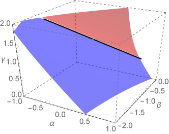
Figure 1: The $(\alpha,\beta,\gamma)$ region which gives the linear-$T$ resistivity in low temperature limit. The (red/blue) surface corresponds to the (class II/class III) solution. The black line, which is the intersection of the red and blue surface, corresponds to the class I. Class IV does not allow the linear-$T$ resistivity.

• class I: The linear-$T$ condition (37) ($(2+d-\theta)/z=1$ in terms of $\alpha,\beta,\gamma$ with (15)) and (16) gives a curve in 3 dimensional $\alpha,\beta,\gamma$ space:

  $$\left(\alpha,\alpha\pm\sqrt{\frac{2}{d(d+1)}},-\alpha\mp\sqrt{\frac{2}{d(d+1)}}d\right)\,,$$ (52)

  which is the black line in Fig. 1.

• class II: The linear-$T$ condition (37) ($(2-\zeta)/z=1$ in terms of $\alpha,\beta,\gamma$ with (18)) defines a surface in 3 dimensional $\alpha,\beta,\gamma$ space:

  $$\left(\alpha,\frac{d^{2}\alpha-d(2\alpha+\gamma)\pm\sqrt{d(2+d((\alpha+\gamma)^{2}-2))}}{d(d-1)},\gamma\right).$$ (53)

  However, the inequality (23) restricts the available surface, which is the red surface in Fig. 1.

• class III: The linear-$T$ condition (37) (($d-\theta-\kappa\beta)/z=1$ in terms of $\alpha,\beta,\gamma$ with (24)) defines a surface in 3 dimensional $\alpha,\beta,\gamma$ space:

  $$\left(\alpha,\frac{3\alpha^{2}+4\alpha\gamma+\gamma^{2}-2-\frac{(\alpha+\gamma)^{2}}{d}}{2(\alpha+\gamma)},\gamma\right).$$ (54)

  However, the inequality (27) restricts the available surface, which is the blue surface in Fig. 1.

• class IV: There is no range. See the explanation below (42).

The potential we consider is valid only for $\beta<0$ because it corresponds to $\kappa>0$ due to (15), (18) and (24) so correctly match the IR potential (49). If we want to consider the case $\beta>0$ we need to reconstruct the potential (47) accordingly. Note also that the sign of $\alpha$ is opposite to $\theta$ so i) for $\alpha>0$ region, the first potential in (47) should be used ii) for $\alpha=0$, the second potential should be used. iii) for $\alpha<0$ region, the third potential in (47) should be used.

4 Linear-$T$ resistivity from low temperature to high temperature

We have fine-gridded the surface in Fig. 1. By trying out all gridded data set ($\alpha,\beta,\gamma$), we have found that, only for a small range of parameters near the parameter set

$$(\alpha,\beta,\gamma)=\left(-\frac{1}{\sqrt{3}},-\frac{2}{\sqrt{3}},\sqrt{3}\right)\ \ \Leftrightarrow\ \ (z,\theta,\zeta)=(3,1,-1)\,,$$ (55)

yields the linear-$T$ resistivity from low temperature to high temperature when the momentum relaxation is strong.

See Fig. 2(a) for the numerical results for this parameter set with a strong momentum relaxation $k/\mu=20$. It is a plot for the resistivity ($\rho$) vs temperature $T$, showing $\rho\sim T^{x}$ with $x\sim 1$.

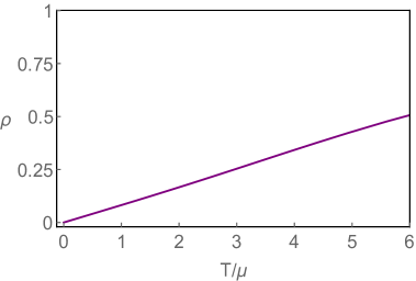
(a) Resistivity ($\rho$) vs Temperature ($T/\mu$)

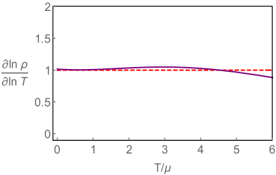
(b) The power $x$ where $\rho\sim T^{x}$. The red dashed line is a guide to the eye.

Figure 2: Resistivity vs temperature: the linear-$T$ resistivity. ($\alpha,\beta,\gamma)=\left(-\frac{1}{\sqrt{3}},-\frac{2}{\sqrt{3}},\sqrt{3}\right)$ (i.e. $(z,\theta,\zeta)=(3,1,-1)$) with large momentum relaxation $k/\mu=20$.

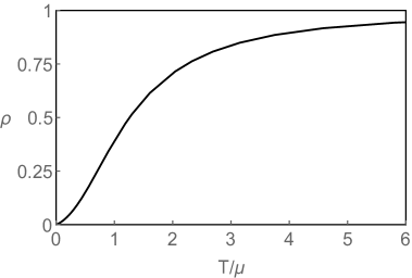
(a) $(\alpha,\beta,\gamma)=\left(\frac{1}{3\sqrt{3}},-\frac{2}{3\sqrt{3}},\frac{5}{3\sqrt{3}}\right)$ (i.e.$\left(z,\theta,\zeta\right)=(5,-1,-3))$) with $k/\mu=10$. The black dot case in Fig. 9(b).

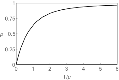
(b) $(\alpha,\beta,\gamma)=\left(0,-\frac{1}{\sqrt{3}},\frac{2}{\sqrt{3}}\right)$ (i.e.$\left(z,\theta,\zeta\right)=(4,0,-2)$) with $k/\mu=10$. The black dot case in Fig. 11.

Figure 3: Resistivity vs temperature: non-linear-$T$ resistivity

To show the value of the exponent $x$ more clearly, we make another plot for $\frac{\partial\ln\rho}{\partial\ln T}$ in Fig. 2(b), where we see $x\sim 1$ for $T/\mu\lesssim 5$. As we explain in section 5.2, a small neighborhood of the point $(-1/\sqrt{3},-2/\sqrt{3},\sqrt{3})$ also exhibits the linear-$T$ resistivity.

For a purpose of comparison, we also show typical plots for non-linear-$T$ resistivity in Fig. 3. The parameters used in Fig. 3 were chosen as the same as the one in Fig. 9(b) and Fig. 11. Note that Fig. 2 corresponds to the third potential ($\alpha<0$) in (47) while Fig. 3(a) and Fig. 3(b) correspond to the first ($\alpha>0$) and second ($\alpha=0$) potential in (47) respectively. It turns out that the third potential or $\alpha<0$ is more advantageous to have a linear-$T$ resistivity than the others. We will discuss about it more in sec. 5.2.

4.1 Momentum relaxation effect

In this subsection, we will show how the momentum relaxation affects the linear-$T$ resistivity behavior in the finite temperature region. In Fig. 4, we find that if the momentum relaxation becomes smaller, the temperature range of the linear-$T$ resistivity becomes shorter.

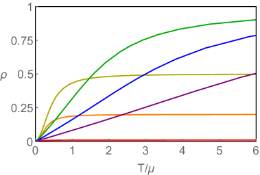
(a) $\rho$ vs $T/\mu$

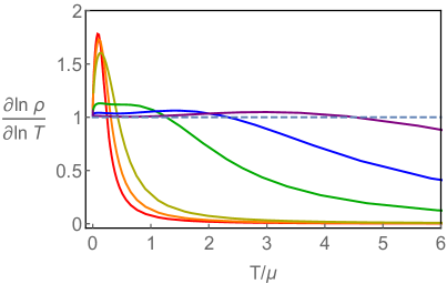
(b) $x$ vs $T/\mu$ ($\rho\sim T^{x}$). The dotted line is for $x=1$.

Figure 4: The temperature dependence of resistivity for $(\alpha,\beta,\gamma)=(-1/\sqrt{3},-2/\sqrt{3},\sqrt{3})$ or $(z,\theta,\zeta)=(3,1,-1)$. The color represents the momentum relaxation strength $k/\mu$: {color($k/\mu$)} = {red(0.1), orange(0.5), yellow(1), green(5), blue(10), purple(20)}.

The different colors in the figures represent different momentum relaxation strength: {red, orange, yellow, green, blue, purple} means $k/\mu=\{1/10,1/2,1,5,10,20$}. From Fig. 4(a), one may think, for all $k/\mu$ we considered, the resistivity looks linear in $T$ for certain range of $T$. However, in fact it is not. By carefully reading off the exponent $x$ in $\rho\sim T^{x}$ in Fig. 4(b), we find that in most cases $x$ becomes quickly deviated from $1$ as $T$ increases from zero. Nevertheless, we stress all the curves in Fig. 4(b) go to $1$ as $T$ goes to zero. This confirms our numerics are consistent with the analytic formula (37). It turns out that the strong momentum relaxation is important to have robust linear-$T$ resistivity up to high temperature. For example, the range for the linear-$T$ resistivity is around up to $T/\mu\sim 5$ for $k/\mu=20$ and $T/\mu\sim 2$ for $k/\mu=10$ as shown in Fig. 4(b).

5 Interpretations of numerical results

In the previous section, we have shown the importance of large momentum relaxation to have a robust linear-$T$ resistivity at finite temperature. To have a better understanding on the mechanism for this observation, in this section, we want to answer the following two questions.

1. (section 5.1) To have a robust linear-$T$ resistivity, which term is important among two terms in (35)? We will show it is the first term, so called the pair creation term.

2. (section 5.2) What are the effects of $\alpha,\beta,$ and $\gamma$ in (46) and (47) on $x$ in $\rho\sim T^{x}$? We will show that

   • Increasing $\alpha$ or $\gamma$ $\Longrightarrow$ increasing $x$.

   • Increasing $\beta$ $\Longrightarrow$ dicreasing $x$.

5.1 First term or second term?

In general, the conductivity (35) consists of two terms. The first term is called the pair creation term ($\sigma_{DC,pc}$) and the second term is called the dissipation term ($\sigma_{DC,diss}$) Gouteraux:2014hca . For $d=2$, (35) reads

$$\sigma_{DC}=\sigma_{DC,pc}+\sigma_{DC,diss}=Z_{H}+\frac{q^{2}}{k^{2}C_{H}J_{H}}\,.$$ (56)

Thus, we may ask which term is responsible for the linear-$T$ resistivity at finite temperature.

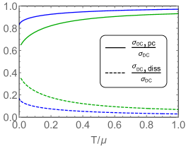
(a) Class I, Eq. (57)

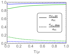
(b) Class II, Eq. (58)

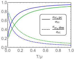
(c) Class III, Eq. (59)

Figure 5: The relative contributions of two terms to the conductivity in (56). The green and blue curves represent $k/\mu=(5,10)$ respectively.

To answer this question we compare $\frac{\sigma_{,DC,pc}}{\sigma_{DC}}$ and $\frac{\sigma_{DC,diss}}{\sigma_{DC}}$ in Fig. 5 for three representative cases

$$\mathrm{Class\ I}:\quad(\alpha,\beta,\gamma)=\left(-\frac{1}{\sqrt{3}},-\frac{2}{\sqrt{3}},\sqrt{3}\right)\,,\quad\left(z,\theta,\zeta\right)=(3,1,-1)\,,$$ (57)

$$\mathrm{Class\ II}:\quad(\alpha,\beta,\gamma)=\left(\frac{1}{\sqrt{5}},-\frac{2}{\sqrt{5}},\frac{4}{\sqrt{5}}\right)\,,\quad(z,\theta,\zeta)=(4,1,-2)\,,$$ (58)

$$\mathrm{Class\ III}:\quad(\alpha,\beta,\gamma)=\left(\frac{1}{\sqrt{5}},-\frac{3}{\sqrt{5}},\frac{3}{\sqrt{5}}\right)\,,\quad(z,\theta,\zeta)=(4,1,-1)\,,$$ (59)

where $(z,\theta,\zeta)$ can be calculated by using (15), (18), (24). We can determine which $(\alpha,\beta,\gamma)$ corresponds to which class by checking the equality and inequalities (16), (23), and (27). For all cases, the resistivity is linear in $T$ in low temperature limit as shown in (37). Class I (57), Class II (58), and Class III (59) are shown in Fig. 5(a), Fiq. 5(b) and Fig. 5(c) respectively. The green and blue curves represent the momentum relaxations, $k/\mu=5$ and $k/\mu=10$.

We find that, in general, at high temperature, the pair creation term contribute more dominantly. It can be understood by more active pair creation at high temperature. At strong momentum relaxation, naively, one may think that the second term is always suppressed because there is $k^{2}$ factor in the denominator. However, this is not obvious because all the other factors $q,C_{H}$, and $J_{H}$ are also implicitly functions of $k$. Indeed, we find that the dissipation term is dominant at low temperature in Class III in Fig. 5(c).

In particular, Fig. 5(a) is for Eq. (57), which exhibits a robust linear-$T$ resistivity. In this case, the larger momentum relaxation is, the more pair creation term is dominant. Thus, we find that the pair creation term, the horizon value of $Z$ ($Z_{H}$), is responsible for the linear-$T$ resistivity at finite temperature.

Furthermore, from Fig. 5(c), we may understand why class III case is hard to exhibit the robust linear-$T$ resistivity at finite temperature. As temperature increases, the dominant mechanism for conductivity is changed: at low temperature, the dissipation term dominates while at high temperature the pair creation term dominates. It will be more difficult to have a universal physics from two different mechanism.

5.2 $\alpha,\beta,\gamma$ dependence

In the previous subsection, we have investigated the effect of the momentum relaxation on the resistivity in finite temperature regime. In this subsection we want to investigate the effect of $\{\alpha,\beta,\gamma\}$ or $\{z,\theta,\zeta\}$ on the resistivity.

Because we found that, in general, the large momentum relaxation is important to have a robust linear-$T$ resistivity, here we fix the momentum relaxation to be large, say $k/\mu=10$. For a systematic study we first need to choose a potential in (47). Thus, we have three cases depending on the sign of $\theta$

$$\theta>0\,,\quad\theta=0\,,\quad\theta<0\,.$$ (60)

This classification is equivalent to

$$\alpha<0\,,\quad\alpha=0\,,\quad\alpha>0\,,$$ (61)

respectively because $\alpha\kappa=-\frac{2\theta}{d}$ with a positive dilaton $\phi$ ($\kappa>0$).

For a given potential we have three classes Class I,II, and III explained in sec.  2.2. The classes are determined by the parameter range. This parameter range and the effect of $\alpha,\beta,\gamma$ on resistivity are best explained by figures, from Fig. 6 to Fig. 12.

Because there are common features in a class of figures (Fig. 6, Fig. 9, Fig. 11) and another class of figures (Fig. 7, Fig. 10, Fig. 12) we explain them here for all of them.

1. (Fig. 6, Fig. 9, Fig. 11) show allowed region of $(\beta,\gamma)$ for a given $\alpha$. The red region, blue region, and the black line between them correspond to class II, class III, and class I respectively.

2. The dotted line in blue and red corresponds to the parameters giving the linear-$T$ resistivity in low temperature limit. Let us imagine that we file up the dashed lines for every $\alpha$. Then, the blue(red) dashed lines form a blue(red) surface in $(\alpha,\beta,\gamma)$ space. This surface is nothing but the surface in Fig. 1. In other words, the dashed lines in figures (Fig. 6, Fig. 9, Fig. 11) are cross-section of Fig. 1 at a given $\alpha$. The region above (below) the dashed line corresponds to $x>1$ ($x<1$), where $x$ is defined in the relation $\rho\sim T^{x}$ in low temperature limit.

3. Therefore, the black dot in (Fig. 6, Fig. 9, Fig. 11) gives the linear-$T$ resistivity as a class I case. Because all the other color dots do not belong to the dotted line they do not give the linear-$T$ resistivity in low temperature limit. We chose these deviated points to investigate the effect of $\alpha,\beta,\gamma$.

4. $\alpha$ increase as the purple dot $\rightarrow$ the black dot $\rightarrow$ the red dot in (Fig. 6 and Fig. 9). This was shown as an arrow in (Fig. 7(a), Fig. 10(a)).

5. $\beta$ increase as the blue dot $\rightarrow$ the black dot $\rightarrow$ the orange dot in (Fig. 6, Fig. 9, Fig. 11). This was shown as an arrow in (Fig. 7(b), Fig. 10(b), Fig. 12(a)).

6. $\gamma$ increase as the dark yellow dot $\rightarrow$ the black dot $\rightarrow$ the green dot in (Fig. 6, Fig. 9, Fig. 11). This was shown as an arrow in (Fig. 7(c), Fig. 10(c), Fig. 12(b)).

7. (Fig. 7, Fig. 10, Fig. 12) shows the exponent $x$ in $\rho\sim T^{x}$. The colors of the curves are chosen to be the same as the colors of the dots in (Fig. 6, Fig. 9, Fig. 11). Recall that the region above (below) the dashed line corresponds to $x>1$ ($x<1$), where $x$ is defined in the relation $\rho\sim T^{x}$ in low temperature limit. Our results show that this tendency remain at finite temperature in general.

8. As a consistency check of our numerics, we have confirmed that the numerical values of $x$ in the limit $T/\mu\rightarrow 0$ for every curve in (Fig. 7, Fig. 10, Fig. 12) agree with the analytic expressions (37) i.e. in the low temperature limit $x\rightarrow 1$ for class I, $x\rightarrow(2-\zeta)/z$ for class II and $x\rightarrow(2-\theta-\kappa\beta)/z$ for class III. For example, in Fig. 7(a), the black, purple, and red curves correspond to class I, II and III respectively. By using the values $(z,\theta,\zeta)=(\frac{21}{5},\frac{7}{5},-1)$ for the purple curve (class II) and $(z,\theta,\zeta,\beta,\kappa)={(\frac{49}{18},\frac{2}{3},-\frac{4}{3},-\frac{2}{\sqrt{3}},\frac{10}{3\sqrt{3}})}$ for the red curve (class III) we find that $x\sim 0.71$ and $x\sim 1.31$ respectively. These agree with our numerical results. One may think that $x\sim 0.71$ is fine but $x\sim 1.31$ looks quite different from the value in our numerics (the red curve in the limit of $T/\mu\rightarrow 0$). However, this is because the red curve belongs to class III. As we showed in Fig. 5(c) in class III the second term of (56) is dominant but the first term’s contribution is still not negligible at low temperature. This contamination by the first term is reflected on our numerics. If we go to extremely low $T/\mu$ we will find a good agreement, which we have checked.

The third potential in (47) ($\alpha<0$ and $\theta>0$)

The reference point is the black dot in Fig. 6(b), which is

$$(\alpha,\beta,\gamma)=(\alpha_{3},\beta_{3},\gamma_{3}):=\left(-\frac{1}{\sqrt{3}},-\frac{2}{\sqrt{3}},\sqrt{3}\right)\ \ \Leftrightarrow\ \ \left(z,\theta,\zeta\right)=(3,1,-1)\,.$$ (62)

Fig. 6 shows the allowed region of ($\beta,\gamma$) for a given $\alpha$: $\alpha=1.4\alpha_{3}$ for Fig. 6(a), $\alpha=\alpha_{3}$ for Fig. 6(b), and $\alpha=0.6\alpha_{3}$ for Fig. 6(c).

For fixed $(\beta,\gamma)=(\beta_{3},\gamma_{3})$, the $\alpha$ decreases from the purple dot ($\alpha=1.4\alpha_{3}$) to the black dot ($\alpha=\alpha_{3}$) and to the red dot ($\alpha=0.6\alpha_{3}$). For these three points the change of $x$ in $\rho\sim T^{x}$ is shown in Fig. 7(a). The value of $x$ increases as $\alpha$ increases at low temperature $T/\mu$ while it does not change at high temperature $T/\mu$.

For fixed $(\alpha,\gamma)=(\alpha_{3},\gamma_{3})$, the $\beta$ increases from the blue dot ($\beta=1.4\beta_{3}$) to the black dot ($\beta=\beta_{3}$) and to the orange dot ($\beta=0.6\beta_{3}$). For these three points the change of $x$ in $\rho\sim T^{x}$ is shown in Fig. 7(b). The value of $x$ decreases as $\beta$ increases in general, but it does not change much in the intermediate temperature range $1<T/\mu<3$.

For fixed $(\alpha,\beta)=(\alpha_{3},\beta_{3})$, the $\gamma$ increases from the dark yellow dot ($\gamma=0.6\gamma_{3}$) to the black dot ($\gamma=\gamma_{3}$) and to the green dot ($\gamma=1.4\gamma_{3}$). For these three points the change of $x$ in $\rho\sim T^{x}$ is shown in Fig. 7(c). The value of $x$ increases as $\gamma$ increases.

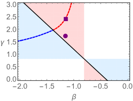
(a) $\alpha=-\frac{14}{10}\frac{1}{\sqrt{3}}$

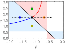
(b) $\alpha=-\frac{1}{\sqrt{3}}$

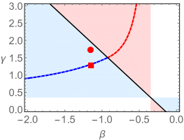
(c) $\alpha=-\frac{6}{10}\frac{1}{\sqrt{3}}$

Figure 6: Allowed region of $(\beta,\gamma)$ for a given $\alpha<0$. In Fig. 7 we show the resistivity for the parameters corresponding to the dots in (a), (b), and (c). See the items 1-5 in sec, 5.2 for the meanings of colors, lines, and dots. In Fig. 8 we show the resistivity for the squares in (a) and (c).

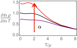
(a) $\alpha$ dependence

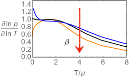
(b) $\beta$ dependence

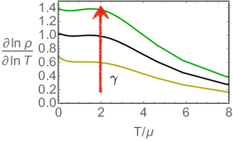
(c) $\gamma$ dependence

Figure 7: The exponent $x$ in $\rho\sim T^{x}$. The colors of the curves are chosen to be the same as the colors of the dots in Fig. 6.

In brief, these can be summrized as follow. The region above (below) the dashed line corresponds to $x>1$ ($x<1$) in the relation $\rho\sim T^{x}$ in low temperature limit. Our results show that this tendency remain at finite temperature in general.

From Fig. 7 one might wonder if we decrease $\alpha$ and increase $\gamma$ the shift-up effect and shift-down effect cancel each other and the linear-$T$ may be obtained again in another point different from the black dot. Indeed, it is true as shown in the purple curve in Fig. 8. By this way, we have found that there is some range of parameters yielding the linear-$T$ resistivity. However, this does not work in the other way, i.e. first increase $\alpha$ and then decrease $\gamma$. See the red curve in Fig. 8. The difference between two ways is the class that the ending point arrives at. The former belongs to class II and the latter belongs to class III. As we showed in Fig. 5(c) the dominant mechanism for conductivity changes as temperature increases in class III, so it is not easy to keep the linear-$T$ resistivity across this change.

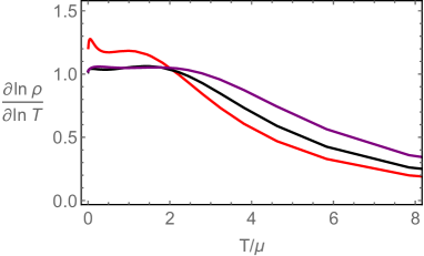
Figure 8: The exponent $x$ in $\rho\sim T^{x}$. The black curve corresponds to the black dot in Fig. 7(a). The purple (red) curve corresponds to the square in Fig. 7(a) (Fig. 7(c)).

Because of very complicated coupled dynamics at finite temperature, it is not easy to have some analytic understanding of our observation. However, we speculate that it may have something to do with the vanishing potential near IR, $V\sim e^{\alpha\phi}$, for $\alpha<0$. For $\alpha\geqslant 0$ the potential will diverge or be constant.

The first potential in (47) ($\alpha>0$ and $\theta<0$)

The reference point is the black dot in Fig. 9(b), which is

$$(\alpha,\beta,\gamma)=(\alpha_{1},\beta_{1},\gamma_{1}):=\left(\frac{1}{3\sqrt{3}},-\frac{2}{3\sqrt{3}},\frac{5}{3\sqrt{3}}\right)\ \ \Leftrightarrow\ \ \left(z,\theta,\zeta\right)=(5,-1,-3)\,.$$ (63)

Fig. 6 shows the allowed region of ($\beta,\gamma$) for a given $\alpha$: $\alpha=0.6\alpha_{1}$ for Fig. 6(a), $\alpha=\alpha_{1}$ for Fig. 6(b), and $\alpha=1.4\alpha_{1}$ for Fig. 6(c).

Similarly to the previous case $\alpha<0(\theta>0)$, we consider six points around the reference black dot. For fixed $(\beta,\gamma)=(\beta_{1},\gamma_{1})$, the $\alpha$ increases from the purple dot ($\alpha=0.6\alpha_{1}$) to the black dot ($\alpha=\alpha_{1}$) and to the red dot ($\alpha=1.4\alpha_{1}$). For fixed $(\alpha,\gamma)=(\alpha_{1},\gamma_{1})$, the $\beta$ increases from the blue dot ($\beta=1.4\beta_{1}$) to the black dot ($\beta=\beta_{1}$) and to the orange dot ($\beta=0.6\beta_{1}$). For fixed $(\alpha,\beta)=(\alpha_{1},\beta_{1})$, the $\gamma$ increases from the dark yellow dot ($\gamma=0.6\gamma_{1}$) to the black dot ($\gamma=\gamma_{1}$) and to the green dot ($\gamma=1.4\gamma_{1}$)

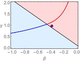
(a) $\alpha=\frac{6}{10}\frac{1}{3\sqrt{3}}$

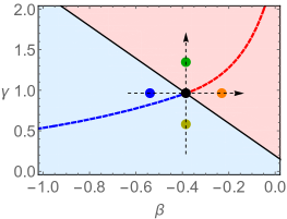
(b) $\alpha=\frac{1}{3\sqrt{3}}$

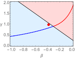
(c) $\alpha=\frac{14}{10}\frac{1}{3\sqrt{3}}$

Figure 9: Allowed $(\beta,\gamma)$ region for a given $\alpha>0$. In Fig. 10 we show the resistivity for the parameters corresponding to the dots in (a), (b), and (c). See the items 1-5 in sec, 5.2 for the meanings of colors, lines, and dots.

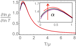
(a) $\alpha$ dependence

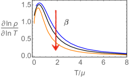
(b) $\beta$ dependence

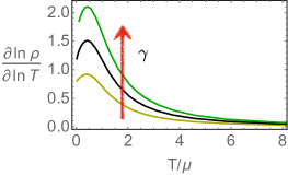
(c) $\gamma$ dependence

Figure 10: The exponent $x$ in $\rho\sim T^{x}$. The colors of the curves are chosen to be the same as the colors of the dots in Fig. 9.

As $\alpha$ increases, $\beta$ decreases, or $\gamma$ increases the curves shift up at finite temperature. See Fig. 10. It is again consistent with the fact that the region above (below) the dashed line corresponds to $x>1$ ($x<1$), where $x$ is defined in the relation $\rho\sim T^{x}$ in low temperature limit.

The second potential in (47) ($\alpha=\theta=0$)

The reference point is the black dot in Fig. 11, which is

$$(\alpha,\beta,\gamma)=(\alpha_{2},\beta_{2},\gamma_{2}):=\left(0,-\frac{1}{\sqrt{3}},\frac{2}{\sqrt{3}}\right)\ \ \Leftrightarrow\ \ \left(z,\theta,\zeta\right)=(4,0,-2)\,.$$ (64)

In this case, there is no change in $\alpha$ since $\alpha=\theta=0$.

For fixed $(\alpha,\gamma)=(0,\gamma_{2})$, the $\beta$ increases from the blue dot ($\beta=1.4\beta_{2}$) to the black dot ($\beta=\beta_{2}$) and to the orange dot ($\beta=0.6\beta_{2}$). For fixed $(\alpha,\beta)=(0,\beta_{2})$, the $\gamma$ increases from the dark yellow dot ($\gamma=0.6\gamma_{2}$) to the black dot ($\gamma=\gamma_{1}$) and to the green dot ($\gamma=1.4\gamma_{1}$). Similarly to other cases, as $\beta$ decreases or $\gamma$ increases the curves shift up at finite temperature. See Fig. 12.

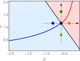
Figure 11: Allowed region of $(\beta,\gamma)$ for $\alpha=0$. In Fig. 12 we show the resistivity for the parameters corresponding to the dots. See the items 1-5 in sec, 5.2 for the meanings of colors, lines, and dots.

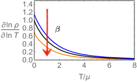
(a) $\beta$ dependence

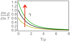
(b) $\gamma$ dependence

Figure 12: The exponent $x$ in $\rho\sim T^{x}$. The colors of the curves are chosen to be the same as the colors of the dots in Fig. 11.

6 Conclusion

In this paper, we studied the linear-$T$ resistivity up to finite temperature in more general cases: axion-dilaton theories or the EMD-Axion models. In order to study resistivity from low to high temperature, we start with the low temperature limit or IR limit. In this limit, resistivity can be analyzed by the scaling geometries supported by the asymptotic potential and couplings in IR (12)

$$V(\phi)\sim V_{0}e^{\alpha\phi}\,,\qquad J(\phi)\sim e^{\beta\phi}\,,\qquad Z(\phi)\sim e^{\gamma\phi}\,.$$ (65)

They are characterized by three parameters $\alpha,\beta,\gamma$, in terms of which, the necessary conditions for the linear-$T$ resistivity has been well studied in Gouteraux:2014hca and summarized in (37). In addition, there are many constraints for $\alpha,\beta,\gamma$ coming from physical conditions. For instance, the specific heat should be positive and our geometry should be stable under small perturbation Gouteraux:2014hca ; Ahn:2017kvc . The constraints are expressed in (16), (23), (27), (31), and (42). Considering all, we have explicitly identified a parameter region which yields the linear-$T$ resistivity in low temperature limit. This region is displayed as a two dimensional surface in three dimensional $\alpha,\beta,\gamma$ space. See Fig. 1.

To study resistivity at finite temperature, not only in the limit of low temperature, we have UV-completed $V(\phi)$ as

$$\begin{split}&V(\phi)=\left\{\begin{array}[]{lll}\frac{2d}{\alpha^{2}}\sinh^{2}\left(\frac{\alpha\phi}{2}\right)+(d+1)d\,,&\text{for}\,\theta<0\,,\\[2.15277pt] (d+1)d\,,&\text{for}\,\theta=0\,,\\[2.15277pt] d\left(\frac{1}{\alpha^{2}}+2\left(d+1\right)\right)\operatorname{sech}(\alpha\phi)-d\left(\frac{1}{\alpha^{2}}+\left(d+1\right)\right)\operatorname{sech}^{2}\left(\alpha\phi\right),&\text{for}\,d>\theta>0\,.\end{array}\right.\end{split}$$ (66)

with the same $J(\phi)$ and $Z(\phi)$ in (65). Contrary to the low temperature limit, no analytic solution is available so we need to resort to numerical analysis.

By fine-gridding the surface of the linear-$T$ resistivity in low temperature limit, in Fig. 1, we have systematically searched the parameters yielding the linear-$T$ resistivity up to high temperature. We found that the point

$$(\alpha,\beta,\gamma)=\left(-\frac{1}{\sqrt{3}},-\frac{2}{\sqrt{3}},\sqrt{3}\right)\ \ \Leftrightarrow\ \ (z,\theta,\zeta)=(3,1,-1)\,,$$ (67)

and its small neighborhood give the linear-$T$ resistivity from low temperature to high temperature if momentum relaxation is strong.

We have found (67) by systematic and hard work by brute force. However, unfortunately, we do not have a deep understanding on the precise physical mechanism for (67) yet. The values (and the size of its neighborhood) will be changed with different UV completions. Thus, our main point is not the values (67) but some qualitative discoveries we have obtained, which will be summarized as follows.

1. Large momentum relaxation is a necessary condition to obtain robust linear-$T$ resistivity from low temperature up to high temperature. See Fig. 4.

2. Among two terms in the conductivity formula (35), the pair-creation term (the first term) is responsible for the linear-$T$ resistivity. In terms of geometry, this is nothing but the horizon value of the coupling $Z(\phi)$ with the Maxwell term for $d=2$ as shown in (2.1) and (56), i.e.

   $$e^{\gamma\phi(r_{h})}=r_{h}^{\gamma\kappa}\,.$$ (68)

   It is a very simple formula. However, it is not easy to have a good intuition, because $r_{h}$ is a functions of ($T,\mu,k$) determined by complicated coupled dynamics of various fields. Only in low temperature limit, $r_{h}\sim T$ so things are simplified.

3. In class III the dominant mechanism for conductivity is switched from the second (dissipation) term to first (pair-creation) term in the conductivity formula, as temperature increases. See Fig. 5. Thus, we may expect that it is not easy to have a universal property, the linear-$T$ resistivity, in class III because of this mechanism change. Indeed, the parameters we found for linear-$T$ resistivity belong to class I and II.

4. In class I, since both deformations (axion and charge) are marginal, the condition $T\ll$ Max($\mu,k$) is enough for the geometry to be captured by the IR scaling geometry. Thus, by increasing momentum relaxation $k$, it is more possible to have a larger range of linear-$T$ resistivity than the other classes. 

5. We also discussed how the conductivity behavior changes as $\alpha,\beta,\gamma$ changes for every potential in section 5.2. We speculate that the third potential in (66) may be favorable for the robust $T$ dependence of resistivity because the potential $V\sim e^{\alpha\phi}$ vanishes near IR for $\alpha<0$. For $\alpha\geqslant 0$ the potential will diverge or be constant.

It has been shown in Jeong:2018tua that the Gubser-Rocha model with linear axion exhibits the linear-$T$ resistivity up to high temperature. This model is also included in our set-up as shown in (50). It corresponds to the parameter set $(\alpha,\beta,\gamma)=(1/\sqrt{3},0,-1/\sqrt{3})$, which is the green dot in Fig. 13. It belongs to the first potential in (66) and class I. In this case, the DC conductivity ($\sigma_{DC}$) is

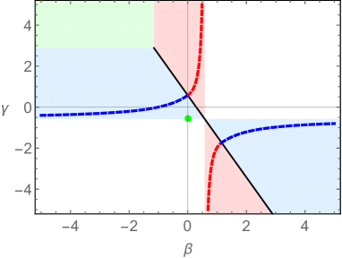
Figure 13: The figure shows allowed ($\beta,\gamma$) region in the case of $\alpha=\frac{1}{\sqrt{3}}$. The black line represent class I case. The red, blue and green region stand for the class II, class III and class IV respectively. The dashed red(blue) line shows $(\alpha,\beta,\gamma)$ for the linear-$T$ resistivity in low temperature limit of class II(class III). The green dot $(\alpha,\beta,\gamma)=(\frac{1}{\sqrt{3}},0,-\frac{1}{\sqrt{3}})$.

$$\sigma_{DC}=\sqrt{1+{\tilde{Q}}}+\frac{\sqrt{1+{\tilde{Q}}}}{(k/\mu)^{2}}\,,$$ (69)

where ${\tilde{Q}}$ is a complicated function of $(T,\mu,k)$. Thus, the first (pair creation) and second (dissipation) term contribute in the same way through ${\tilde{Q}}$. However, it has been shown that the resistivity is linear in $T$ up to high temperature only for large momentum relaxation, $k/\mu\gg 1$, so the first term dominates. This agrees with what we have found in this paper.

In order to identify the power $x$ in $\rho\sim T^{x}$ in a more precise way we made a plot of $\partial\ln\rho/\partial\ln T$. This method is good enough to find a linear-$T$ behavior all the way from zero $T$ to high $T$. However, if there is a residual resistivity at zero $T$ (i.e. $T=\mathrm{constant}+T^{x}$) or if there is the linear-$T$ resistivity after some temperature $T_{1}$ (i.e. for $T>T_{1}>0$, $T=\mathrm{constant}+T^{x}$), our measure $\partial\ln\rho/\partial\ln T$ may not be able to capture it. Thus, in such more relaxed conditions, which may be relevant for some phenomenology (for example, Cooper603 ), there may be more parameter regime allowing the linear-$T$ resistivity in our model.

Investigating conductivity at high temperature involves full bulk geometry so it depends on UV-completion of potential and couplings in general. In this paper, as a first step, we used a kind of minimal UV completion, in the sense that the potential $V$ depends on only one parameter $\alpha$. As reviewed in Appendix A other UV completions are also possible. It will be interesting if we can find more conditions to constrain UV completion from other phenomenological input or theoretical consistency such as a top-down approach. Or, from phenomenological perspective, we may ask what kind of UV completion can allow the linear-$T$ resistivity up to high temperature.

Appendix A UV completion

In this appendix, we explain how to obtain the potential for UV completion in a little more detail. In principle, there are many ways to construct $V,Z$, and $J$ satisfying (12)

$$J(\phi)\sim e^{\beta\phi}\,,\qquad Z(\phi)\sim e^{\gamma\phi}\,,\qquad V(\phi)\sim V_{0}e^{\alpha\phi}\,,$$ (70)

in IR for scaling geometry, and (43) and (44)

$$V(\phi)=\frac{(d+1)d}{\ell_{AdS}^{2}}-\frac{1}{2}m^{2}\phi^{2}+\cdots,$$ (71)

$$Z(\phi)=1+\cdots\,,\quad J(\phi)=1+\cdots,$$ (72)

in UV for asymptotically AdS space. In other words, for $V(\phi)$,

$$V(0)=-2\Lambda=\frac{(d+1)d}{\ell_{AdS}^{2}}\,,\qquad V^{\prime}(0)=0\,,\qquad V^{\prime\prime}(0)=-m^{2}=\frac{-\Delta(\Delta-d-1)}{\ell_{AdS}^{2}}\,,$$ (73)

where $\Delta$ is the conformal dimension of the dual operator of $\phi$. $\phi\rightarrow\infty$ in IR and $\phi\rightarrow 0$ in UV. For simplicity, in this paper, we choose a minimal potentials studied in Ling2017 :

$$Z(\phi)=e^{\gamma\phi}\,,\qquad J(\phi)=e^{\beta\phi}\,,$$ (74)

and three cases for $V(\phi)$

$$\begin{split}&V(\phi)=\left\{\begin{array}[]{lll}\frac{2d}{\alpha^{2}}\sinh^{2}\left(\frac{\alpha\phi}{2}\right)+(d+1)d\,,&\text{for}\,\theta<0\,,\\[2.15277pt] (d+1)d\,,&\text{for}\,\theta=0\,,\\[2.15277pt] d\left(\frac{1}{\alpha^{2}}+2\left(d+1\right)\right)\operatorname{sech}(\alpha\phi)-d\left(\frac{1}{\alpha^{2}}+\left(d+1\right)\right)\operatorname{sech}^{2}\left(\alpha\phi\right),&\text{for}\,d>\theta>0\,,\end{array}\right.\end{split}$$ (75)

where we set $\ell_{AdS}=1$ for simplicity.

One way to determine the potential is to introduce several exponential terms as follows:

$$V(\phi)=V_{0}e^{\alpha\phi}+V_{1}e^{\alpha_{1}\phi}+V_{2}e^{\alpha_{2}\phi}+\cdots+V_{n}e^{\alpha_{n}\phi}\,.$$ (76)

The simplest way is to use only first two terms, of which parameters $(V_{0},V_{1},\alpha_{1})$ will be completely fixed by three conditions. Instead, we may choose three terms which is considered in Kiritsis:2015oxa :

$$V(\phi)=V_{0}e^{\alpha\phi}+V_{1}e^{\alpha_{1}\phi}+V_{2}e^{\alpha_{2}\phi}\,.$$ (77)

There are five free parameters $(V_{0},V_{1},\alpha_{1},V_{2},\alpha_{2})$ and we have only three constraints. To fix two parameters we choose $\alpha_{2}=0$ and $V_{0}=\frac{d}{2\alpha^{2}}$. There are two motivation for this choice: i) it avoids the log behavior of $\phi$ in UV  Kiritsis:2015oxa , ii) it can include the Gubser-Rocha model by choosing $(\alpha,\beta,\gamma)=(1/\sqrt{3},0,-1/\sqrt{3})$ (see (50)). Furthermore, we also choose $m^{2}=-d$ so the potential becomes only a function of $\alpha$. By these choices, the potential $V(\phi)$ in (77) becomes

$$V(\phi)=\frac{2d}{\alpha^{2}}\sinh^{2}\frac{\alpha\phi}{2}+(d+1)d\,.$$ (78)

Because we want to have a form $V(\phi)\sim V_{0}e^{\alpha\phi}$ in IR, (78) is valid for $\alpha>0$ since $\phi>0$. Otherwise, the dominant term in IR will be $V(\phi)\sim V_{0}e^{-\alpha\phi}$ or constant.

Although we may construct the potential by using 3 exponential terms (77) for $\alpha<0$, we use a different ‘building block’ to construct the potential:

$$V(\phi)=\frac{V_{0}}{2}\operatorname{sech}(\alpha\phi)+V_{1}\operatorname{sech}^{2}(\alpha\phi)\,,$$ (79)

where $1/2$ in $V_{0}/2$ is chosen to match the IR condition at $\alpha\phi\rightarrow-\infty$ (70). With this $\operatorname{sech}(\alpha\phi)$ form, one of the UV condition, the second of (73) is automatically satisfied since $\phi\rightarrow 0$ in UV. Thus the remaining free parameters $V_{0}$ and $V_{1}$ are fixed by the first and third constraints in (73):

$$V(\phi)=\left((d+1)d-\frac{V_{0}}{2}\right)\left(1-\tanh^{2}(\alpha\phi)\right)+\frac{V_{0}}{2\cosh(\alpha\phi)}\,,$$ (80)

where $V_{0}=2d(-{m^{2}}/{(d\alpha^{2})}+2d+2)$. Finally with the choice of $m^{2}=-d$, which is the same as the first potential in Eq. (47), the potential becomes a function of $\alpha$ only.

For $\alpha=0$ case, we choose the constant potential:

$$V(\phi)=(d+1)d\,,$$ (81)

where $m=0$. Even with this constant potential the field $\phi$ still runs nontrivially due to a non trivial $J$ and $Z$.

References

- (1) S. A. Hartnoll, A. Lucas and S. Sachdev, Holographic quantum matter, 1612.07324.
- (2) M. Blake and A. Donos, Quantum Critical Transport and the Hall Angle, 1406.1659.
- (3) Z. Zhou, J.-P. Wu and Y. Ling, DC and Hall conductivity in holographic massive Einstein-Maxwell-Dilaton gravity, JHEP 08 (2015) 067, [1504.00535].
- (4) K.-Y. Kim, K. K. Kim, Y. Seo and S.-J. Sin, Thermoelectric Conductivities at Finite Magnetic Field and the Nernst Effect, JHEP 07 (2015) 027, [1502.05386].
- (5) Z.-N. Chen, X.-H. Ge, S.-Y. Wu, G.-H. Yang and H.-S. Zhang, Magnetothermoelectric DC conductivities from holography models with hyperscaling factor in Lifshitz spacetime, Nucl. Phys. B924 (2017) 387–405, [1709.08428].
- (6) E. Blauvelt, S. Cremonini, A. Hoover, L. Li and S. Waskie, Holographic model for the anomalous scalings of the cuprates, Phys. Rev. D97 (2018) 061901, [1710.01326].
- (7) B. S. Kim, E. Kiritsis and C. Panagopoulos, Strange metal behavior from the Light-Cone AdS Black Hole, 1012.3464.
- (8) C. Homes, S. Dordevic, M. Strongin, D. Bonn, R. Liang et al., Universal scaling relation in high-temperature superconductors, Nature 430 (2004) 539, [cond-mat/0404216].
- (9) J. Zaanen, Superconductivity: Why the temperature is high, Nature 430 (07, 2004) 512–513.
- (10) J. Erdmenger, B. Herwerth, S. Klug, R. Meyer and K. Schalm, S-Wave Superconductivity in Anisotropic Holographic Insulators, JHEP 05 (2015) 094, [1501.07615].
- (11) K.-Y. Kim, K. K. Kim and M. Park, A Simple Holographic Superconductor with Momentum Relaxation, JHEP 04 (2015) 152, [1501.00446].
- (12) K. K. Kim, M. Park and K.-Y. Kim, Ward identity and Homes’ law in a holographic superconductor with momentum relaxation, JHEP 10 (2016) 041, [1604.06205].
- (13) K.-Y. Kim and C. Niu, Homes’ law in Holographic Superconductor with Q-lattices, JHEP 10 (2016) 144, [1608.04653].
- (14) J. Zaanen, Y.-W. Sun, Y. Liu and K. Schalm, Holographic Duality in Condensed Matter Physics. Cambridge Univ. Press, 2015.
- (15) M. Ammon and J. Erdmenger, Gauge/gravity duality. Cambridge Univ. Pr., Cambridge, UK, 2015.
- (16) C. Charmousis, B. Gouteraux, B. S. Kim, E. Kiritsis and R. Meyer, Effective Holographic Theories for low-temperature condensed matter systems, JHEP 11 (2010) 151, [1005.4690].
- (17) R. A. Davison, K. Schalm and J. Zaanen, Holographic duality and the resistivity of strange metals, Phys. Rev. B89 (2014) 245116, [1311.2451].
- (18) B. Goutéraux, Charge transport in holography with momentum dissipation, JHEP 1404 (2014) 181, [1401.5436].
- (19) X.-H. Ge, Y. Tian, S.-Y. Wu, S.-F. Wu and S.-F. Wu, Linear and quadratic in temperature resistivity from holography, JHEP 11 (2016) 128, [1606.07905].
- (20) S. Cremonini, H.-S. Liu, H. Lu and C. N. Pope, DC Conductivities from Non-Relativistic Scaling Geometries with Momentum Dissipation, JHEP 04 (2017) 009, [1608.04394].
- (21) H.-S. Jeong, Y. Ahn, D. Ahn, C. Niu, W.-J. Li and K.-Y. Kim, Thermal diffusivity and butterfly velocity in anisotropic Q-Lattice models, JHEP 01 (2018) 140, [1708.08822].
- (22) A. Salvio, Transitions in Dilaton Holography with Global or Local Symmetries, JHEP 03 (2013) 136, [1302.4898].
- (23) A. Donos and J. P. Gauntlett, Thermoelectric DC conductivities from black hole horizons, JHEP 11 (2014) 081, [1406.4742].
- (24) K.-Y. Kim, K. K. Kim, Y. Seo and S.-J. Sin, Coherent/incoherent metal transition in a holographic model, JHEP 12 (2014) 170, [1409.8346].
- (25) K.-Y. Kim, K. K. Kim, Y. Seo and S.-J. Sin, Gauge Invariance and Holographic Renormalization, Phys. Lett. B749 (2015) 108–114, [1502.02100].
- (26) H.-S. Jeong, K.-Y. Kim and C. Niu, Linear- resistivity at high temperature, JHEP 10 (2018) 191, [1806.07739].
- (27) S. S. Gubser and F. D. Rocha, Peculiar properties of a charged dilatonic black hole in , Phys.Rev. D81 (2010) 046001, [0911.2898].
- (28) Z. Zhou, Y. Ling and J.-P. Wu, Holographic incoherent transport in Einstein-Maxwell-dilaton Gravity, Phys. Rev. D94 (2016) 106015, [1512.01434].
- (29) K.-Y. Kim and C. Niu, Diffusion and Butterfly Velocity at Finite Density, JHEP 06 (2017) 030, [1704.00947].
- (30) S. A. Hartnoll, Theory of universal incoherent metallic transport, 1405.3651.
- (31) L. V. Delacrtaz, B. Goutraux, S. A. Hartnoll and A. Karlsson, Bad Metals from Fluctuating Density Waves, SciPost Phys. 3 (2017) 025, [1612.04381].
- (32) A. Amoretti, D. Aren, B. Goutraux and D. Musso, Effective holographic theory of charge density waves, Phys. Rev. D97 (2018) 086017, [1711.06610].
- (33) A. Amoretti, D. Aren, B. Goutraux and D. Musso, DC resistivity of quantum critical, charge density wave states from gauge-gravity duality, Phys. Rev. Lett. 120 (2018) 171603, [1712.07994].
- (34) R. A. Davison, S. A. Gentle and B. Goutraux, Slow relaxation and diffusion in holographic quantum critical phases, 1808.05659.
- (35) R. A. Davison, S. A. Gentle and B. Goutraux, Impact of irrelevant deformations on thermodynamics and transport in holographic quantum critical states, 1812.11060.
- (36) E. Kiritsis and J. Ren, On Holographic Insulators and Supersolids, JHEP 09 (2015) 168, [1503.03481].
- (37) Y. Ling, Z. Xian and Z. Zhou, Power Law of Shear Viscosity in Einstein-Maxwell-Dilaton-Axion model, Chin. Phys. C41 (2017) 023104, [1610.08823].
- (38) J. Bhattacharya, S. Cremonini and B. Goutéraux, Intermediate scalings in holographic RG flows and conductivities, 1409.4797.
- (39) Y. Ling, Z. Xian and Z. Zhou, Power law of shear viscosity in einstein-maxwell-dilaton-axion model, Chinese Physics C 41 (feb, 2017) 023104.
- (40) R. A. Davison and B. Goutéraux, Dissecting holographic conductivities, JHEP 09 (2015) 090, [1505.05092].
- (41) B. Gouteraux and E. Kiritsis, Generalized Holographic Quantum Criticality at Finite Density, JHEP 12 (2011) 036, [1107.2116].
- (42) R. A. Cooper, Y. Wang, B. Vignolle, O. J. Lipscombe, S. M. Hayden, Y. Tanabe et al., Anomalous criticality in the electrical resistivity of la2–xsrxcuo4, Science 323 (2009) 603–607, [https://science.sciencemag.org/content/323/5914/603.full.pdf].