COLLABORATIVE FILTERING AND MULTI-LABEL CLASSIFICATION WITH MATRIX FACTORIZATION

Abstract

Machine learning techniques for Recommendation System and Classification has become a prime focus of research to tackle the problem of information overload. Recommender Systems are software tools that aim at making informed decisions about the services that a user may like. Recommender Systems can be broadly classified into two categories namely, content-based filtering and collaborative filtering. In content-based filtering, users and items are represented using a set of features (profile) and an item is recommended by finding the similarity between the user and item profile. On the other hand in collaborative filtering, the user-item association is obtained based on the preferences of the user given so far and the preference information of other users.

Classification technique deals with the categorization of a data object into one of the several predefined classes. The majority of the methods for supervised machine learning proceeds from a formal setting in which data objects (instances) are represented in the form of feature vectors wherein each object is associated with a unique class label from a set of disjoint class labels. Depending on the total number of disjoint classes, a learning task is categorized as binary classification or multi-class classification. In the multi-label classification problem, unlike the traditional multi-class classification setting, each instance can be simultaneously associated with a subset of labels.

In both recommendation and classification problem, the initial assumption is that the input-data is in the form of matrices which are inherently low rank. The key technical challenge involved in designing new algorithms for recommendation and classification is dependent on how well one can handle the huge and sparse matrices which usually has thousands to millions of rows and which are usually noisy. Recent years have witnessed extensive applications of low-rank linear factor model for exploiting the complex relationships that exist in such data matrices. The goal is to learn a low-dimensional embedding where the data object can be represented with a small number of features. Matrix factorization methods have attracted significant attention for learning the low-rank latent factors. The focus of thesis is on the development of novel techniques for collaborative filtering and multi-label classification.

In maximum margin matrix factorization scheme of collaborative filtering, ratings matrix with multiple discrete values is treated by specially extending hinge loss function to suit multiple levels. We view this process as analogous to extending two-class classifier to a unified multi-class classifier. Alternatively, multi-class classifier can be built by arranging multiple two- class classifiers in a hierarchical manner. We investigate this aspect for collaborative filtering and propose a novel method of constructing a hierarchical bi-level maximum margin matrix factorization to handle matrix completion of ordinal rating matrix. The advantages of the proposed method over other matrix factorization based collaborative filtering methods are given by detailed experimental analysis. We also observe that there could be several possible alternative criteria to formulate the factorization problem of discrete ordinal rating matrix, other than the maximum margin criterion. Taking the cue from the alternative formulation of support vector machines, a novel loss function is derived by considering proximity as an alternative criterion instead of margin maximization criterion for matrix factorization framework. We validate our hypothesis by conducting experiments on real and synthetic datasets.

We extended the concept of matrix factorization for yet another important problem of machine learning namely multi-label classification which deals with the classification of data with multiple labels. We propose a novel piecewise-linear embedding method with a low-rank constraint on parametrization to capture nonlinear intrinsic relationships that exist in the original feature and label space. Extensive comparative studies to validate the effectiveness of the proposed method against the state-of-the-art multi-label learning approaches is given through detailed experimental analysis. We also study the embedding of labels together with the group information with an objective to build an efficient multi-label classifier. We assume the existence of a low-dimensional space onto which the feature vectors and label vectors can be embedded. We ensure that labels belonging to the same group share the same sparsity pattern in their low-rank representations. We perform comparative analysis which manifests the superiority of our proposed method over state-of-art algorithms for multi-label learning.

Contents

1. 1 Introduction
   1. 1.1 Contributions of the Thesis
   2. 1.2 Structure of the Thesis
   3. 1.3 Publications of the Thesis
2. 2 Foundational Concepts
   1. 2.1 Matrix Factorization
   2. 2.2 Loss Function
      1. 2.2.1 Binary Loss Function:
      2. 2.2.2 Discrete Ordinal Loss Function
      3. 2.2.3 Real-valued Loss Function
   3. 2.3 Regularization
   4. 2.4 Collaborative filtering with Matrix Factorization
   5. 2.5 Multi-label Classification with Matrix Factorization
3. 3 Collaborative Filtering Using Hierarchical Matrix Factorizations
   1. 3.1 Introduction
   2. 3.2 Bi-level MMMF
   3. 3.3 Multi-level MMMF
   4. 3.4 HMF- The Proposed Method

List of Tables

1. 3.1 Bi-level matrix $Y$
2. 3.2 Latent factor matrices corresponding to $Y$.
3. 3.5 Real-valued prediction corresponding to bi-level matrix Y.
4. 3.6 Hinge loss corresponding to observed entries in Y.
5. 3.7 Smooth hinge loss corresponding to observed entries in Y.
6. 3.8 Runnning example.
7. 3.13 Real-valued prediction corresponding to ordinal rating matrix $Y$.
8. 3.14 Ordinal rating matrix Y
9. 3.15 Runnning example.
10. 3.20 Partially complete matrix after stage 1
11. 3.21 Runnning example.
12. 3.26 Partially complete matrix after stage 2
13. 3.27 Runnning example.
14. 3.32 Partially complete matrix after stage 3
15. 3.33 Runnning example.
16. 3.38 Partially complete matrix after stage 4
17. 3.39 Complete matrix computed by HMF

List of Figures

1. 3.1 Geometrical interpretation of bi-level matrix factorization.
2. 3.2 Loss function values for the hinge
3. 3.3 Loss function values for the smooth hinge
4. 3.4 Convergence graph of BMMMF with different initial points
5. 3.5 Classification by MMMF for the $i$th user
6. 3.6 Classification by MMMF for $i$th user
7. 3.7 Convergence graph of MMMF with different initial points
8. 3.4 HMF- The Proposed Method

CF	Collaborative Filtering
FE	Feature Space Embedding
GroPLE	Group Preserving Label Embedding for Multi-Label Classification
HMF	Hierarchical Matrix Factorization
LE	Label Space Embedding
MF	Matrix Factorization
MLC	Multi-label Classification
MLC-HMF	Multi-label Classification Using Hierarchical Embedding
MMMF	Maximum Margin Matrix Factorization
PMMMF	Proximal Maximum Margin Matrix Factorization

This is to certify that the thesis entitled “Collaborative Filtering and Multi-Label Classification with Matrix Factorization” submitted by Vikas Kumar bearing Reg. No. 14MCPC07 in partial fulfillment of the requirements for the award of Doctor of Philosophy in Computer Science is a bonafide work carried out by him under our supervision and guidance.

This thesis is free from plagiarism and has not been submitted previously in part or in full to this or any other university or institution for the award of any degree or diploma. The student has the following publications before submission of the thesis for adjudication and has produced evidence for the same.

1. "Collaborative Filtering Using Multiple Binary Maximum Margin Matrix Factorizations." Information Sciences 380 (2017): 1-11.

2. "Proximal Maximum Margin Matrix Factorization for Collaborative Filtering." Pattern Recognition Letters 86 (2017): 62-67.

3. "Multi-label Classification Using Hierarchical Embedding." Expert Systems with Applications 91 (2018): 263-269.

Further, the student has passed the following courses towards fulfillment of coursework requirement for Ph.D.

Course Code	Name	Credits	Pass/Fail
CS 801	Data Structures and Algorithms	4	Pass
CS 802	Operating Systems and Programming	4	Pass
AI 810	Metaheuristic Techniques	4	Pass
AI 852	Learning & Reasoning	4	Pass

Prof. Arun K Pujari Supervisor	Prof. Vineet Padmanabhan Supervisor
Prof. K. Narayana Murthy Dean, School of Computer and Information Sciences

I, Vikas Kumar, hereby declare that this thesis entitled “Collaborative Filtering and Multi-Label Classification with Matrix Factorization” submitted by me under the guidance and supervision of Prof. Arun K Pujari and Prof. Vineet Padmanabhan is a bonafide research work. I also declare that it has not been submitted previously in part or in full to this university or any other university or institution for the award of any degree or diploma.

Date:

Name:    Vikas Kumar
                                                              Signature of the Student:

Reg. No. 14MCPC07

Dedicated to my parents and family members, for everything what I am today and above all, devoted to The Almighty God!

Chapter 1   Introduction

With the advent of technology and high usage of modern equipment/ devices, large amounts of data are being generated world over. We now stand at the brink of data-driven transformation where the data can be harnessed to derive meaningful insights that can help organizations for better functioning as well as assist the user in his/ her decision making process. Examples include (a) suggesting the right choice of products to a user or identifying the most appropriate customers for a product (b) assisting an organization in classifying the users for better serviceability etc.

The vast amount of accumulated data is a crucial competitive asset and can be tailored to satisfy an individual’s/ organization’s needs. However, the crucial challenge here is in the processing of the data. The amount of data is enormous and therefore requires a large amount of time to explore all of them. For example, if one has to purchase an item, he/ she needs to process all the information to select which items meet their needs. To avoid the information overload, we need some assistance in the form of recommendation or classification in our day to day life. For instance, when we are purchasing an electronic gadget, we usually rely on the suggestions of friends who shares similar tastes. Similarly, when we are planning to invest in equity funds, we need some assistance to differentiate between different equity based on their features before we decide to invest. In the recent past, machine learning techniques are most commonly used to understand the nature of data so as to help in reducing the burden on individuals in the decision making process. Machine learning techniques for Recommendation and Classification has become a prime focus of research to tackle the problem of information overload.

Recommendation (Recommender) Systems are software tools that aim at making informed decisions about the services that a user may like [sarwar2002incremental, koren2011advances, lu2015recommender]. Given a list of users, items and user-item interactions (ratings), Recommender System predicts the score/ affinity of item $j$ for user $i$ and thereby helps in understanding the user behaviour which in turn can be used to make personalized recommendations. Examples include classic recommendation tasks such as recommending books, movies, music etc., as well as new web-based applications such as predicting preferred news articles, websites etc. Recommender Systems can be broadly classified into two categories namely, content-based filtering and collaborative filtering[lu2015recommender]. In content-based filtering, users and items are represented using a set of features (profile) and an item is recommended by finding the similarity between the user and the item profile. In the case of collaborative filtering the user-item association is obtained based on the preferences of the user given so far and the preference information of other users.

Classification is a supervised learning technique which deals with the categorization of a data object into one of the several predefined classes. Majority of the methods for supervised machine learning proceeds from a formal setting in which the data objects (instances) are represented in the form of feature vectors wherein each object is associated with a unique class label from a set of disjoint class labels $L$, $|L|>1$. Depending on the total number of disjoint classes in $L$, a learning task is categorized as binary classification (when $|L|=2$) or multi-class classification (when $|L|>2$) [read2009classifier, tsoumakas2007random]. In this thesis, we are focusing on a special class of classification problem called multi-label classification. Unlike the traditional classification setting, in multi-label classification problem, each instance can be simultaneously associated with a subset of labels. For example, in image classification, an image can be simultaneously tagged with a subset of labels such as natural, valley, mountain etc. Similarly, in document classification, a document can simultaneously belong to Computer Science and Physics. The multi-label classification task aims at building a model that can automatically tag a new example with the most relevant subset of class labels.

In this thesis we focus on developing novel techniques for collaborative filtering and multi-label classification. It should be kept in mind that in both recommendation and classification problem the data is actually organized in matrix form. For example, in collaborative filtering, users preferences on items can be represented as a matrix, whose rows represent users, columns represent items, and each element of the matrix represent the preference of a user for an item. Similarly, in multi-label classification problem, the set of data objects and their corresponding label vectors can be represented as a matrix. The data object can be represented as a row of the feature matrix and the associated label vector can be represented as the corresponding row of label matrix. The key technical challenge involved in designing new algorithms for recommendation and classification is dependent on how well one can handle the huge and sparse matrices which usually has thousands and millions of rows and which are usually noisy.

Recent years have witnessed extensive applications of low-rank linear factor models for exploiting the complex relationships existing in such data matrices. The goal is to learn a low-dimensional embedding where the data object can be represented with a small number of features. For instance, in the case of collaborative filtering, the idea is to learn low-dimensional latent factors for every user and item. Similarly, in multi-label classification the goal of low-rank factor model learning is to embed the feature and label vector to a low dimensional space so that the intrinsic relationship in the original space can be captured. Matrix factorization (MF) methods have attracted significant attention in the areas of computer vision [cao2015low, cao2016robust], pattern recognition [wang2015subspace, zhang2015ensemble], image processing [fevotte2015nonlinear, haeffele2014structured], information retrieval [kim2015simultaneous, tang2016supervised] and signal processing [vu2016combining, wang2014discriminative] for learning low-rank latent factor models. The objective of MF is to learn low-rank latent factor matrices $U$ and $V$ so as to simultaneously approximate the observed entries under some loss measure. Here, the interpretation of factor matrices $U$ and $V$ are application dependent. We present a brief discussion on matrix factorization approach for collaborative filtering and multi-label classification.

Matrix factorization is just one way of doing collaborative filtering (CF) wherein it is possible to discover the latent features underlying the interactions between two different kinds of entities (user/ item). CF approaches also assume that a user’s preference on an item is determined by a small number of factors and how each of those factors applies to the user and the item (low dimensional linear factor model). The intuition behind using matrix factorization is that there should be some latent features that determine how a user rates an item. It is possible that two users would highly rate a movie if it belongs to a particular genre like action/ comedy. Discovering these latent features definitely helps in predicting the rating with respect to a certain user and a certain item because the features associated with the user should match with the features associated with the item. It is also the case that in trying to discover the different features, an assumption is made that the number of features would be smaller than the number of users and the number of items. The idea is that it is not reasonable to assume that each user is associated with a unique feature in which case it would be absurd to make any recommendations because each of these users would not be interested in the items rated by other users.

The discussion above shows that CF can be formulated as a MF problem in the sense that, in a $d$-factor model, given a rating matrix $Y\in\mathbb{R}^{N\times M}$ the idea is to find two low-rank matrices $U\in\mathbb{R}^{N\times d}$ and $V\in\mathbb{R}^{M\times d}$ such that $Y\approx UV^{T}$ where $d$ is a parameter. Each entry $y_{ij}\in\{0,1,2,\dots,R\}$ in $Y$, defines the preference given by $i$th user for $j$th item. $y_{ij}=0$, indicates that the user has not given any preference for $j$th item and $R$ is the total level of ratings. The goal is to predict the preference for all items for which the user’s preference is unobserved. The $i$th row of $U$ represents the latent factor of the $i$th user and the $j$th row of $V$ represents the latent feature of the $j$th item. The prediction for $y_{ij}$ can be achieved by the linear combination of the $i$th row of $U$ with the $j$th row of $V$ i.e.

$$y_{ij}=\sum_{p=1}^{d}U_{ip}V_{jp}=U_{i}V^{T}_{j}$$ (1.1)

The outcome of matrix factorization method is a low-rank, dense matrix $X$ which is an approximation of the given sparse rating matrix Y. Here X is computed as $X=UV^{T}$.

Multi-label classification can be seen as a generalization of single label classification where an instance is associated with a unique class label from a set of disjoint labels $L$. Formally, given $N$ training examples in the form of a pair of feature matrix $X$ and label matrix $Y$ where each example $x_{i}\in\mathbb{R}^{D},1\leq i\leq N$, is a row of $X$ and its associated labels $y_{i}\in\{-1,+1\}^{L}$ is the corresponding row of $Y$, the task of multi-label classification is to learn a parameterization $h:\mathbb{R}^{D}\rightarrow\{-1,+1\}^{L}$ that maps each instance to a set of labels. Multi-label classification has applications in many areas such as machine learning  [babbar2017dismec, yen2016pd, read2009classifier, zhang2006multilabel], computer vision  [liu2015low, wang2016cnn, cabral2011matrix, boutell2004learning] and data mining  [nam2014large, zhou2014activity, tsoumakas2007random, schapire2000boostexter]. Multi-label classification is nowadays applied to massive data sets of considerable size and under such conditions, time- and space-efficient implementations of learning algorithms is of major concern. For example, there are millions of articles available on Wikipedia each tagged with a set of labels and in most of the cases, the author of an article associates very few labels which they know from a broad set of relevant labels.

To cope with the challenge of exponential-sized output space, exploiting intrinsic information in feature and label spaces has been the major thrust of research in recent years and use of parametrization and embedding have been the prime focus. Researchers have studied several aspects of embedding which include label embedding, feature embedding, dimensionality reduction and feature selection. These approaches differ from one another in their capability to capture other intrinsic properties such as label correlation and local invariance. To glean out the potentially hidden dynamics that exists in the original space, most of the embedding based approaches focus on learning a low-dimensional representation for the original feature (label) vector. There are two strategies of embedding for exploiting inter-label correlation; (1) Feature Space Embedding (FE); and (2) Label Space Embedding (LE). FE aims to design a projection function which can map the instance in the original feature space to an embedded space and then a mapping is learnt from the embedded space to the label space. The second approach is to transform the label vectors to an embedded space, followed by the association between feature vectors and embedded label space for classification purpose.

In recent years, matrix factorization based approach which aims at determining two matrices $U$ and $V$ is frequently used to achieve the FE and LE. In FE, the goal is to transform each $D$-dimensional feature vector (a row of matrix $X$) from the original feature space to a $L$-dimensional label vector (corresponding row in $Y$) and usually the mapping is achieved through a linear transformation matrix $W\in\mathbb{R}^{D\times L}$. The MF based approach assumes that the label matrix $Y$ is of low-rank due to the presence of similar labels and thereby models the inter-label correlation implicitly using low-rank constraints on the transformation matrix $W$. The transformation matrix $W$ is approximated using the product of two latent factor matrices $U$ and $V$. The matrix $U$ acts as a transformation matrix which transforms the data from the original feature space to an embedded space and the matrix $V$ can be interpreted as the decoding matrix from the embedded space to the label space.

In LE, the goal is to transform each $L$-dimensional label vector (a row of matrix $Y$) from the original label space to a $d$-dimensional embedded vector. Thereafter, a predictive model is trained from the original feature space to the embedded space. With proper decoding process that maps the projected data back to the original label space, the task of multi-label prediction is achieved. The LE approach based on MF aims at approximating the label matrix $Y$ as a product of two matrices $U$ and $V$ with the assumption that the label matrix exhibits a low-rank structure. The $i$th row of matrix $U$ can be viewed as the embedded representation of the label vector associated with the $i$th instance and the matrix $V$ can be viewed as the decoding matrix from the embedded space to the label space.

1.1   Contributions of the Thesis

The major contributions of the thesis are as follows. In maximum margin matrix factorization scheme (a variant of basic matrix factorization method), ratings matrix with multiple discrete values is treated by specially extending hinge loss function to suit multiple levels. We view this process as analogous to extending two-class classifier to a unified multi-class classifier. Alternatively, multi-class classifier can be built by arranging multiple two- class classifiers in a hierarchical manner. We investigate this aspect for collaborative filtering and propose a novel method of constructing a hierarchical bi-level maximum margin matrix factorization to handle matrix completion of ordinal rating matrix [KUMAR20171].

We observe that there could be several possible alternative criteria to formulate the factorization problem of discrete ordinal rating matrix, other than the maximum margin criterion. Taking a cue from the alternative formulation of support vector machines, a novel loss function is derived by considering proximity as an alternative criterion instead of margin maximization criterion for matrix factorization framework [KUMAR201762].

We extended the concept of matrix factorization for yet another important problem of machine learning namely multi-label classification which deals with the classification of data with multiple labels. We propose a novel piecewise-linear embedding method with a low-rank constraint on the parametrization to capture nonlinear intrinsic relationships that exist in the original feature and label space [KUMAR2018263].

We study the embedding of labels together with the group information with an objective to build an efficient multi-label classifier. We assume the existence of a low-dimensional space onto which the feature vectors and label vectors can be embedded. We ensure that labels belonging to the same group share the same sparsity pattern in their low-rank representations.

1.2   Structure of the Thesis

The thesis is organized as follows. In Chapter $2$, we start our discussion with an introductory discussion on matrix factorization and the associated optimization problem formulation. Thereafter we discuss some common loss functions used in matrix factorization to measure the deviation between the observed data and the corresponding approximation. We also discuss several ways of norm regularization which is needed to avoid overfitting in matrix factorization models. In the later part of the chapter we discuss at length the application of matrix of factorization techniques in collaborative filtering and multi-label classification.

Chapter $3$ starts with a discussion on bi-level maximum margin matrix factorization (MMMF) which we subsequently use in our proposed algorithm. We carry out a deep investigation of the well known maximum margin matrix factorization technique for discrete ordinal rating matrix. This investigation led us to propose a novel and efficient algorithm called HMF (Hierarchical Matrix Factorization) for constructing a hierarchical bi-level maximum margin matrix factorization method to handle matrix completion of ordinal rating matrix. The advantages of HMF over other matrix factorization based collaborative filtering methods are given by detailed experimental analysis at the end of the chapter.

Chapter $4$ introduces a novel method termed as PMMMF (Proximal Maximum Margin Matrix Factorization) for factorization of matrix with discrete ordinal ratings. Our work is motivated by the notion of Proximal SVMs (PSVMs) [li2015multia, Fung2001] for binary classification where two parallel planes are generated, one for each class, unlike the standard SVMs [vapnik2013nature, burges1998tutorial, mangasarian1999generalized]. Taking the cue from here, we make an attempt to introduce a new loss function based on the proximity criterion instead of margin maximization criterion in the context of matrix factorization. We validate our hypothesis by conducting experiments on real and synthetic datasets.

Chapter $5$ extended the concept of matrix factorization for yet another important problem in machine learning namely multi-label classification. We visualize matrix factorization as a kind of low-dimensional embedding of the data which can be practically relevant when a matrix is viewed as a transformation of data from one space to the other. At the beginning of the chapter we discuss briefly about the traditional approach of multi-label classification and establish a bridge between multi-label classification and matrix factorization. We present a novel multi-label classification method, called MLC-HMF (Multi-label Classification using Hierarchical Embedding), which learns piecewise-linear embedding with a low-rank constraint on parametrization to capture nonlinear intrinsic relationships that exist in the original feature and label space. Extensive comparative studies to validate the effectiveness of the proposed method against the state-of-the-art multi-label learning approaches is discussed in the experimental section.

In Chapter $6$, we study the embedding of labels together with group information with an objective to build an efficient multi-label classifier. We assume the existence of a low-dimensional space onto which the feature vectors and label vectors can be embedded. In order to achieve this, we address three sub-problems namely; (1) Identification of groups of labels; (2) Embedding of label vectors to a low rank-space so that the sparsity characteristic of individual groups remains invariant; and (3) Determining a linear mapping that embeds the feature vectors onto the same set of points, as in stage 2, in the low-rank space. At the end, we perform comparative analysis which manifests the superiority of our proposed method over state-of-art algorithms for multi-label learning.

We conclude the thesis with a discussion on future directions in Chapter $7$.

1.3   Publications of the Thesis

1. Vikas Kumar, Arun K Pujari, Sandeep Kumar Sahu, Venkateswara Rao Kagita, Vineet Padmanabhan. "Collaborative Filtering Using Multiple Binary Maximum Margin Matrix Factorizations." Information Sciences 380 (2017): 1-11.

2. Vikas Kumar, Arun K Pujari, Sandeep Kumar Sahu, Venkateswara Rao Kagita, Vineet Padmanabhan. "Proximal Maximum Margin Matrix Factorization for Collaborative Filtering." Pattern Recognition Letters 86 (2017): 62-67.

3. Vikas Kumar, Arun K Pujari, Vineet Padmanabhan, Sandeep Kumar Sahu,Venkateswara Rao Kagita. "Multi-label Classification Using Hierarchical Embedding." Expert Systems with Applications 91 (2018): 263-269.

4. Vikas Kumar, Arun K Pujari, Vineet Padmanabhan, Venkateswara Rao Kagita. "Group Preserving Label Embedding for Multi-Label Classification." PatternRecognition, Under Review.

Chapter 2   Foundational Concepts

In majority of data-analysis tasks, the datasets are naturally organized in matrix form. For example, in collaborative filtering, users preferences on items can be represented as a matrix, whose rows represent users, columns represent items, and each element of the matrix represent the preference of a user for an item. In a clustering problem, a row of the matrix represents data object (instance) and the columns represent associated features (attributes). In image inpainting problem, an image can be represented by a matrix where each entry of the matrix corresponds to pixel values. Similarly, in document analysis, a set of document can be represented as a matrix wherein the rows represent terms and the columns represent documents. Each entry represents the frequency of the associated terms in a particular document.

Recent advances in many data-analysis tasks have been focused on finding a meaningful (simplified) representation of the original data matrix. A simplified representation typically helps in better understanding the structure, relationship within the data or attributes and retrieving the hidden information that exists in the original data matrix. Matrix Factorization (MF) methods have attracted significant attention for finding the latent (hidden) structure from the original data matrix. Given an original matrix $Y\in\mathbb{R}^{N\times M}$, MF aims at determining two matrices $U\in\mathbb{R}^{N\times d}$ and $V\in\mathbb{R}^{M\times d}$ such that $Y\approx UV^{T}$ where the inner dimension $d$ is called the numerical rank of the matrix. The numerical rank is much smaller than $M$ and $N$, and hence, factorization allows the matrix to be stored inexpensively. Here, the interpretation of factor matrices $U$ and $V$ are application dependent. For example, in collaborative filtering, given that $Y$ is a $N\times M$ size user-item rating matrix, MF aims at determining the latent factor representation of users and items. The $i$th row of $U$ represents the latent factor of the $i$th user and the $j$th row of $V$ represents the latent feature of the $j$th item [koren2009matrix, rennie2005fast, mnih2007probabilistic, koren2008factorization, salakhutdinov2007restricted]. In a clustering problem with $M$ data points (columns of $Y$) and $d$ cluster, the $j$th column of $U$ can be interpreted as the representative of the $j$th cluster and $i$th column of $V^{T}$ can be visualized as the reconstruction weights of the $i$th data point from those representatives [eriksson2012high, xu2003document, liu2013multi, wang2008semi].

The MF field is too vast to cover and there are many research directions one can pursue starting from theoretical aspects to application-oriented aspects. In this thesis, we focus our discussion on two special applications of matrix factorization, namely collaborative filtering [koren2009matrix, rennie2005fast, mnih2007probabilistic, koren2008factorization, salakhutdinov2007restricted] and multi-label classification [cabral2011matrix, wicker2012multi, balasubramanian2012landmark, jing2015semi]. The purpose of this chapter is to introduce the basic matrix factorization framework and concepts which will be used throughout the thesis (Section 2.1). In Section 2.2, we discuss some of the common loss functions used in MF to measure the deviation between the observed data and corresponding approximation. We briefly discuss the different ways to avoid overfitting in MF model in Section 2.3. In Section 2.4 and 2.5, we explore how matrix factorization can be applied to interesting applications of machine learning namely collaborative filtering and multi-label classification, respectively.

2.1   Matrix Factorization

Matrix factorization is a key technique employed for many real-world applications wherein the objective is to select $U$ and $V$ among all the matrices that fit the given data and the one with the lowest rank is preferred. In most applications, the task that needs to be performed is not just to compute any factorization, but also to enforce additional constraints on the factors $U$ and $V$. The matrix factorization problem can be formally defined as follows:

Definition 1 (Matrix Factorization).

Given a data matrix $Y\in\mathbb{R}^{N\times M}$, matrix factorization aims at determining two matrices $U\in\mathbb{R}^{N\times d}$ and $V\in\mathbb{R}^{M\times d}$ such that $Y\approx UV^{T}$ where the inner dimension $d$ is called the numerical rank of the matrix. The numerical rank is much smaller than $M$ and $N$, and hence, factorization allows the matrix to be stored inexpensively. $X=UV^{T}$ is called as low-rank approximation of $Y$.

A common formulation for this problem is a regularized loss problem which can be given as follows.

$$\underset{U,V}{min}\;\ell(Y,U,V)+\lambda R(U,V)$$ (2.1)

where $Y$ is the data matrix, $X=UV^{T}$ is its low-rank approximation, $\ell(\cdot)$ is a loss function that measures how well $X$ approximates $Y$, and $R(\cdot)$ is a regularization function that promotes various desired properties in $X$ (low-rank, sparsity, group-sparsity, etc.). When $\ell(\cdot)$ and $R(\cdot)$ are convex functions of $X$ (equivalently, of $U$ and $V$) the above problem can be solved efficiently. The loss function $\ell(Y,U,V)$ can further be decmposed into the sum of pairwise discrepancy between the observed entries and their corresponding prediction, that is, $\ell(Y,U,V)=\sum_{i=1}^{N}{\sum_{j=1}^{M}\ell(y_{ij},U_{i},V_{j})}$, where $y_{ij}$ is the $ij$th entry of the matrix $Y$ and $U_{i}$, the $i$th row of $U$, represent the latent feature vector of $i$th user and $V_{j}$, the $j$th row of $V$, represent the latent feature vector of $j$th item. There have been umpteen number of proposals for factorizing a matrix and these differ, by and large, among themselves in defining the loss function and the regularization function. The structure of the latent factors depends on the types of loss (cost) functions and the constraints imposed on the factor matrices. In the following subsections, we present a brief literature review of the major loss functions and regularizations.

2.2   Loss Function

Loss function $\ell:Y\times Y\rightarrow\mathbb{R}$ in MF model is used to measure the discrepancy between the observed entry and the corresponding prediction. Based on the types of observed data, the loss function in MF can be roughly grouped into three categories: (1) Loss function for Binary data; (2) Loss function for Discrete ordinal data; and (3) Loss function for Real-valued data.

2.2.1   Binary Loss Function:

For a binary data matrix $Y=[y_{ij}]$ where the entries are restricted to take only two values $y_{ij}\in\{+1,-1\}$, we review some of the important loss functions such as zero-one loss, hinge loss, smooth hinge loss, modified least square and logistic loss [rennie2005loss] in the following subsections.

Zero-One Loss : The zero-one loss is a standard loss function to measure the penalty for an incorrect prediction which takes only two values zero or one. For a given observed entry $y_{ij}$ and the corresponding prediction $U_{i}V_{j}^{T}$, zero-one loss is defined as

$$\ell(z)=\begin{cases}0&\text{if $z~{}\geq~{}0$;}\\ 1&\text{otherwise,}\end{cases}$$ (2.2)

where $z=y_{ij}(U_{i}V_{j}^{T})$.

Hinge Loss: There are two major drawbacks with zero-one loss (1) Minimizing objective function involving zero-one loss is difficult to optimize as the function is non-convex; (2) It is insensitive to the magnitude of prediction whereas in general, when the entries are binary, the magnitude of score $y_{ij}(U_{i}V_{j}^{T})$ represent the confidence in our prediction. The hinge loss is a convex upper bound on zero-one error [globerson2006nightmare] and sensitive to the magnitude of prediction. In the case of classification with large confidence (margin), hinge loss is the most preferred loss function and is defined as

$$\ell(z)=\begin{cases}$0$&\text{if z $\geq$ 1;}\\ 1-z&\text{otherwise.}\end{cases}$$ (2.3)

Smooth Hinge Loss: Hinge loss, $h(z)$ is non-differentiable at $z=1$ and very sensitive to outliers [rennie2005fast]. An alternative of hinge loss is proposed in [rennie2005loss] called smooth hinge and is defined as

$$\ell(z)=\begin{cases}0&\text{if z $\geq$ 1;}\\ \frac{1}{2}(1-z)^{2}&\text{if $0<z<1$;}\\ \frac{1}{2}-z&\text{otherwise.}\end{cases}$$ (2.4)

Smooth Hinge shares many properties with hinge loss and is insensitive to outliers. A detailed discussion about hinge and smooth hinge loss is given in Chapter $3$.

Modified Square Loss: In [zhang2001text], the hinge function is replaced by a smoother quadratic function to make the derivative smooth. The modified square loss is defined as

$$\ell(z)=\begin{cases}0&\text{if z $\geq$ 1;}\\ (1-z)^{2}&\text{otherwise.}\\ \end{cases}$$ (2.5)

Logistic Loss: The logistic loss function is strictly convex function which enjoys properties similar to that of the hinge loss [mairal2009supervised]. The logistic loss is defined as

$$\ell(z)=\log(1+\exp^{-z}).$$ (2.6)

2.2.2   Discrete Ordinal Loss Function

For a discrete ordinal matrix $Y=[y_{ij}]$ where entries are no more like and dislike but can be any value from a discrete range, that is, $y_{ij}\in\{1,2,\dots,R\}$, there is need to extend binary class loss function to multi-class loss function. There are two major approaches for extending loss function for binary class classification to multi-class classification. The first approach is to directly solve a multi-class problem by modifying the binary class objective function by adding a constraint to it for every class as suggested in [rennie2005loss] [zhang2013multicategory] . The second approach is to decompose the multi-class classification problem into a series of independent binary class classification problems as given in [byun2002applications].

To extend binary loss function to multi-class setting, most of the approaches define a set of threshold values $\theta_{1}<\theta_{1}<\dots<R-1$ such that the real line is divided into $R$ regions. The region defined by threshold $\theta_{q-1}$ and $\theta_{q}$ corresponds to rating $q$ [rennie2005loss]. For simplicity of notation, we assume $\theta_{0}=-\infty$ and $\theta_{R}=+\infty$. There are different approaches for constructing a loss function based on a set of threshold values such as immediate-threshold and all-threshold [rennie2005loss]. For each observed entry and corresponding prediction pair $(y_{ij},U_{i}V_{j}^{T})$, the immediate-threshold based approach calculates the loss as the sum of immediate-threshold violation.

$$\ell(y_{ij},U_{i}V_{j}^{T})=\ell(U_{i}V_{j}^{T}-\theta_{i,y_{ij}-1})~{}+~{}\ell(\theta_{i,y_{ij}}-U_{i}V_{j}^{T})$$ (2.7)

On the other hand, all-threshold loss is calculated as the sum of loss for all threshold which is the cost of crossing multiple rating-boundaries and is defined as

$$\ell(U_{i}V_{j}^{T},y_{ij})=\sum_{r=1}^{y_{ij}-1}{\ell(U_{i}V_{j}^{T}-\theta_{i,r})}+\sum_{r=y_{ij}}^{R-1}{\ell(\theta_{i,r}-U_{i}V_{j}^{T})}.$$ (2.8)

2.2.3   Real-valued Loss Function

For a real-valued data matrix $Y=[y_{ij}]$ where the entries are in real-valued domain $\mathbb{R}$, we review some of the important loss functions such as square-loss [paatero1997], KL-divergence [lee2001], $\beta$-divergence [cichocki2006csiszar] and Itakura-Saito divergence [fevotte2009nonnegative] loss. These are given in the following subsections.

Squared Loss: The square loss is the most common loss function used for real-valued prediction. The penalty for misclassification is calculated as the square distance between the observed entry and the corresponding prediction. The square loss is defined as

$$\ell(y_{ij},\hat{y}_{ij})=(y_{ij}-\hat{y}_{ij})^{2}$$ (2.9)

where $\hat{y}_{ij}=U_{i}V_{j}^{T}$.

Kullback-Leibler Divergence Loss: The KL-divergence loss also know as I-divergence loss is the measure of information loss when $U_{i}V_{j}^{T}$ is used as an approximate to $y_{ij}$. The KL-divergence loss is defined as

$$\ell(y_{ij},\hat{y}_{ij})=y_{ij}\ln\frac{y_{ij}}{\hat{y}_{ij}}-y_{ij}+\hat{y}_{ij}.$$ (2.10)

Itakura-Saito Divergence: Itakura and Saito [fevotte2009nonnegative] is obtained from the the maximum likelihood (ML) estimation. The loss function is defined as

$$\ell(y_{ij},\hat{y}_{ij})=\frac{y_{ij}}{\hat{y}_{ij}}-y_{ij}\ln\frac{y_{ij}}{\hat{y}_{ij}}-1.$$ (2.11)

$\beta$-Divergence Loss: Cichocki et al. [cichocki2006csiszar] proposed a generalized family of loss function called $\beta$-divergence defined as

$$\ell(y_{ij},U_{i},V_{j})=\begin{cases}\frac{y_{ij}^{\beta}}{\beta(\beta-1)}+\frac{\hat{y}_{ij}^{\beta}}{\beta}-\frac{y_{ij}\hat{y}_{ij}^{\beta-1}}{\beta-1}&\text{if $\beta\in\mathbb{R}\setminus\{0,1\}$;}\\ y_{ij}\ln\frac{y_{ij}}{\hat{y}_{ij}}-y_{ij}+\hat{y}_{ij}&\text{if $\beta=1$;}\\ \frac{y_{ij}}{\hat{y}_{ij}}-y_{ij}\ln\frac{y_{ij}}{\hat{y}_{ij}}-1&\text{if $\beta=0$,}\\ \end{cases}$$ (2.12)

where $\beta\geq 0$ is a generalization parameter. At limitng case $\beta=0$ and $\beta=1$, the $\beta$-divergence corresponds to Itakura-Saito divergence and Kullback-Leibler divergence, respectively. The squared loss can be obtained as a special case at $\beta=2$.

2.3   Regularization

Most of the machine learning algorithms suffer from the problem of overfitting where the model fits the training data too well but have poor generalization capability for new data. Thus, a proper technique should be adopted to avoid overfitting of the training data. In MF community, to make the model unbiased i.e., to avoid the model to fit only with a particular dataset, many researchers have tried with different regularization terms along with some loss function [koren2010collaborative, paterek2007improving, takacs2007major, koren2009matrix]. Regularization is not only used to prevent overfitting but also to achieve different structural representation of the latent factors. Several methods based on norm regularization has been proposed in the literature which includes $\ell_{1}$, $\ell_{2}$ and $\ell_{2,1}$.

$\ell_{1}$ Norm: The $\ell_{1}$ norm, also know as sparsity inducing norm, is used to produce sparse latent factors and thus avoids overfitting by retaining only the useful factors. In effect, this implies that most units take values close to zero while only few take significantly non-zero values. For a a given matrix $A$, the $\ell_{1}$ norm is defined as

$$\|A\|_{1}=\sum_{ij}|a_{ij}|.$$ (2.13)

$\ell_{2}$ Norm: The most popular and widely investigated regularization term used in MF model is $\ell_{2}$ norm which is also known as Frobenius norm. For a given matrix $A$, the $\ell_{2}$ norm is defined as

$$\|A\|_{F}=\sqrt{\sum_{ij}a^{2}_{ij}}$$ (2.14)

where $\|\cdot\|_{2}$ is the $\ell_{2}$ norm of a matrix. Minimizing the objective function containing the $\ell_{2}$ norm as regularization term gives two benefits 1) It avoids overfitting by penalizing the large latent factor values. 2) Approximating the target matrix with low-rank factor matrix is a typical non-convex optimization problem and in fact, the $\ell_{2}$ norm has also been suggested as a convex surrogate for the rank in control applications [fazel2001rank, rennie2005fast].

$\ell_{2,1}$ Norm: The $\ell_{2,1}$ norm also known as group sparsity norm is used to induce a sparse representation at the level of groups. For a given matrix $A$, the $\ell_{2,1}$ norm is defined as

$$\|A\|_{2,1}=\sum_{i=1}^{n}{\sqrt{\sum_{j=1}^{m}A_{ij}^{2}}}.$$ (2.15)

2.4   Collaborative filtering with Matrix Factorization

In collaborative filtering, the goal is to infer user preferences for items based on his/ her previously given preference and a large collection of preferences of other users. Given a partially observed $N\times M$ user-item rating matrix $Y$ with $N$ number of users and $M$ number of items the goal is to predict unobserved preference of users for items. The collaborative filtering problem can be formally defined as follows:

Definition 2 (Collaborative Filtering).

Let $Y$ be a $N\times M$ size user-item rating matrix and $\Omega$ be the set of observed entries. For each $(i,j)\in\Omega$, the entry $y_{ij}\in\{1,2,\dots,R\}$ defines the preference of $i$th user for $j$th item. For each $(i,j)\notin\Omega$, $y_{ij}=0$ indicates that preference of $i$th user for $j$th item is not available (unsampled entry). Given a partially observed rating matrix $Y\in\mathbb{R}^{N\times M}$, the goal is to predict $y_{ij}$ for $(i,j)\notin\Omega$.

Matrix factorization is a key technique employed for completion of user-item rating matrix wherein the objective is to learn low-rank (or low-norm) latent factors $U$ (for users) and $V$ (for items) so as to simultaneously approximate the observed entries under some loss measure and predict the unobserved entries. There are various ways of doing so. It is shown in [lee1999learning] that to approximate $Y$, the entries in the factor matrix $U$ and $V$ need to be non-negative so that only additive combination factors are allowed. The basic idea is to learn factor matrices $U$ and $V$ in such a way that, the squared sum distance between the observed entry and corresponding prediction is minimized. The optimization problem is formulated as

$$\underset{U\geq 0,V\geq 0}{min}J(U,V)=\sum_{(i,j)\in\Omega}{(y_{ij}-U_{i}V_{j}^{T})^{2}}.$$ (2.16)

Singular value decomposition (SVD) is used in [sarwar2002incremental] to learn the factor matrices $U$ and $V$. The key technical challenge when SVD is applied to sparse matrices is that it suffers from severe overfitting. When SVD factorization is applied on sparse data, error function needs to be modified so as to consider only the observed ratings by setting the non-observed entries to zero. This minor modification results in a non-convex optimization problem. Instead of minimizing the rank of a matrix, maximum margin matrix factorization (MMMF) [srebro2004maximum] proposed by srebro et al. aims at minimizing the Froebenius norms of $U$ and $V$, resulting in convex optimization problems. It is shown that MMMF can be formulated as a semi-definite programming (SDP) problem and solved using standard SDP solvers. However, current SDP solvers can only handle MMMF problems on matrices of dimensionality up to a few hundred. Hence, a direct gradient based optimization method for MMMF is proposed in [rennie2005fast] to make fast collaborative prediction. The detailed discussion about MMMF is given in Chapter 3. To further improve the performance of MMMF, in [decoste2006collaborative], MMMF is casted using ensemble methods which includes bagging and random weight seeding. MMMF was further extended in [weimer2008improving] by introducing offset terms, item dependent regularization and a graph kernel on the recommender graph. In [xu2012nonparametric], a noparametric Bayesian-style MMMF was proposed that utilizes nonparametric techniques to resolve the unknown number of latent factors in MMMF model [weimer2008improving][rennie2005fast][decoste2006collaborative]. A probabilistic interpretation of MMMF was presented in [xu2013fast] model through data augmentation.

The proposal of MMMF hinges heavily on extended hinge loss function. Research on different loss functions and their extension to handle multiple classes has not attracted much attention of researchers though there are some important proposals [liu2011hard]. MMMF has become a very popular research topic since its publication and several extensions have been proposed [decoste2006collaborative, weimer2008improving, xu2012nonparametric, xu2013fast]. There has also been some research on matrix factorization on binary or bi-level preferences [Volkovs2015]. But many view binary preference as a special case of matrix factorization with discrete ratings. In [zhong2012contextual] the rating matrix is decomposed hierarchically by grouping similar users and items together, and each sub-matrix is factorized locally. To the best of our knowledge, there is no research on hierarchical MMMF.

2.5   Multi-label Classification with Matrix Factorization

In machine learning and statistics, the classification problem is concerned with the assignment of a class (category) to a data object (instance) from a given set of discrete classes. For example, classifying a document into one of the several known categories such as sports, crime, business, politics etc. In a traditional classification problem, data objects are represented in the form of feature vectors, each associated with a unique class label from a set of disjoint class labels $L$, $|L|>1$. Depending on the total number of disjoint classes in $L$, a learning task is categorized as binary classification (when $|L|=2$) or multi-class classification (when $|L|>2$) [sorower2010literature]. However, in many real-word classification tasks, data object can be simultaneously associated with one or more than one class in $L$. For example, a document can simultaneously belong to more than one class such as politics and business. The objective of multi-label classification (MLC) is to build a classifier that can automatically tag an example with the most relevant subset of labels. This problem can be seen as a generalization of the single label classification where an instance is associated with a unique class label from a set of disjoint labels $L$. The multi-label classification problem can be formally defined as follows:

Definition 3 (Multi-label Classification).

Given $N$ training examples in the form of a pair of feature matrix $X$ and label matrix $Y$ where each example $x_{i}\in\mathbb{R}^{D},1\leq i\leq N$, is a row of $X$ and its associated labels $y_{i}\in\{-1,1\}^{L}$ is the corresponding row of $Y$. The $+1$ entry at the $j$th coordinate of vector $y_{i}$ indicates the presence of label $j$ in data point $x_{i}$. The task of multi-label classification is to learn a parametrization $h:\mathbb{R}^{D}\rightarrow\{-1,1\}^{L}$ that maps each instance (or, a feature vector) to a set of labels (a label vector).

MLC is a major research area in the machine learning community and finds application in several domains such as computer vision [cabral2011matrix, boutell2004learning], data mining [tsoumakas2007random, schapire2000boostexter] and text classification [zhang2006multilabel, schapire2000boostexter]. Due to the exponential size of the output space, exploiting intrinsic information in the feature and the label space has been the major thrust of research in recent years and the use of parametrization and embedding techniques have been the prime focus in MLC. The embedding based approach assumes that there exists a low-dimensional space onto which the given set of feature vectors and/ or label vectors can be embedded. The embedding strategies can be grouped into two categories namely; (1) Feature space embedding; and (2) Label space embedding. Feature space embedding aims to design a projection function which can map the instance in the original feature space to the label space. On the other hand, the label space embedding approach transform the label vectors to an embedded space via linear or local non-linear embeddings, followed by the association between feature vectors and embedded label space for classification purpose. With proper decoding process that maps the projected data back to the original label space, the task of multi-label prediction is achieved [hsu2009multi, rai2015large, tai2012multilabel]. We present a brief review of the FE and LE approaches for multi-label classification. The detailed discussion is given in Chapter LABEL:mlchmfChapter.

Given $N$ training examples in the form of a pair of feature matrix $X$ and label matrix $Y$ where each example $x_{i}\in\mathbb{R}^{D},1\leq i\leq N$, is a row of $X$ and its associated labels $y_{i}\in\{-1,+1\}^{L}$ is the corresponding row of $Y$, the goal of FE is to learn a transformation matrix $W\in\mathbb{R}^{D\times L}$ which maps instances feature space to label space. This approach requires $D\times L$ parameter to model the classification problem, which will be expensive when $D$ and $L$ are large [yu2014large]. In  [yu2014large] a generic empirical risk minimization (ERM) framework is used with low-rank constraint on linear parametrization $W=UV^{T}$, where $U\in\mathbb{R}^{D\times d}$ and $V\in\mathbb{R}^{L\times d}$ are of rank $d\ll D$. The problem can be restated as follows.

$$\underset{U,V}{min}\;\ell(Y,XUV^{T})+\frac{\lambda}{2}(\|U\|_{F}^{2}+\|V\|_{F}^{2})\\$$ (2.17)

where $\|\cdot\|_{F}$ is Frobenius norm. The formulation in Eq. (2.17) can capture the intrinsic information of both feature and label space. It can also be seen as a joint learning framework in which dimensionality reduction and multi-label classification are performed simultaneously [ji2009linear, yu2016semisupervised].

The matrix factorization (MF) based approach for LE aims at determining two matrices $U\in\mathbb{R}^{N\times d}$ and $V\in\mathbb{R}^{d\times L}$ [bhatia2015sparse, xu2016robust]. The matrix $U$ can be viewed as the basis matrix, while the matrix $V$ can be treated as the coefficient matrix and a common formulation is the following optimization problem.

$$\underset{U,V}{min}\;\ell(Y,U,V)+\lambda R(U,V)\\$$ (2.18)

where $\ell(\cdot)$ is a loss function that measures how well $UV$ approximates $Y$, $R(\cdot)$ is a regularization function that promotes various desired properties in $U$ and $V$ (sparsity, group-sparsity, etc.) and the constant $\lambda\geq 0$ is the regularization parameter which controls the extent of regularization. In [lin2014multi], a MF based approach is used to learn the label encoding and decoding matrix simultaneously. The problem is formulated as follows.

$$\underset{U,V}{min}~{}\|Y-UV\|_{F}^{2}+\alpha\Psi(X,U)$$ (2.19)

where $U\in\mathbb{R}^{N\times d}$ is the code matrix, $V\in\mathbb{R}^{d\times L}$ is the decoding matrix, $\Psi(X,U)$ is used to make $U$ feature-aware by considering correlations between $X$ and $U$ as side information and the constant $\alpha\geq 0$ is the trade-off parameter.

Chapter 3   Collaborative Filtering Using Hierarchical Matrix Factorizations

In the previous chapter, we discussed the basic matrix factorization model and the associated formulation of matrix factorization as an optimization problem. We have also discussed at length the application of matrix of factorization techniques in collaborative filtering and multi-label classification. In this chapter, we elaborate on those basics and propose a matrix factorization based collaborative filtering approach.

3.1   Introduction

In this chapter, we describe the proposed method, termed as HMF (Hierarchical Matrix Factorization). HMF is a novel method for constructing a hierarchical bi-level maximum margin matrix factorization to handle matrix completion of ordinal rating matrix. The proposed method draws motivation from research on multi-class classification. There are two major approaches of extending two-class classifiers to multi-class classifiers. The first approach explicitly reformulates the classifier, resulting in a unified multiclass optimization problem (embedded technique). The second approach (combinational technique) is to decompose a multiclass problem into multiple, independently trained, binary classification problems and to combine them appropriately so as to form a multiclass classifier. In maximum margin matrix factorization (MMMF) [rennie2005fast], the authors adopted embedded approach by extending bi-level hinge loss to multi-level cases.

Combinational techniques have been very popular and successful as they all exhibit some relative advantages over embedded techniques and this prompts us to question whether some sort of combinational approach can be employed in the context of MMMF. There are several approaches in combinational techniques and these are One-Against-All (OAA) [hsu2002comparison, rifkin2004defense, weston1998multi], One-Against-One (OAO) [debnath2004decision, hsu2002comparison] etc. HMF falls into the category of OAA approach with a difference. The OAA approach of classification employs one binary classifier for each class against all other classes. In the present context ‘class’ corresponds to the number of ordinal ranks. Interestingly, since the ranks are ordered, in the present case, OAA strategy is used by taking advantage of the ordering of ’classes’. Unlike the traditional OAA strategy, (which means that one bi-level matrix factorization to be used for rank $q$ as one label (say, $-1$) and all other ranks as the other label (say, $+1$)), here we employ for each rank $q$, all ranks below $q$ as $-1$ and all ranks above $q$ as $+1$.

MMMF and HMF, like any other matrix factorization methods, use latent factor model approach. The latent factor model is concerned with learning from limited observations, latent factor vector $U_{i}$ for each user and latent factor vector $V_{j}$ for each item, such that the dot product of $U_{i}$ and $V_{j}$ gives the ranking of user $i$ for item $j$. In MMMF, besides learning the latent factors, the set of thresholds also needs to be learned. It is assumed that there are $R-1$ thresholds $\theta_{i,r}$ for each user $i$ ($R$ is the number of ordinal values or number of ranks). Thus, the rating of user $i$ for item $j$ is decided by comparing the dot product of $U_{i}$ and $V_{j}$ with each $\theta_{i,r}$. Thus, the fundamental assumption of MMMF is that the latent factor vectors determine the properties of users and items and the threshold values capture the characteristics of rating. HMF differs from MMMF on this principle. The underlying principle of HMF is that the latent factors of users and items are going to be different, if the users’ likes or dislikes cutoff thresholds are different. The latent factors are different according to situations. For instance, the latent factors when ranks above $q$ are identified as likes is different from situations wherein the ranks above $q+1$ are identified as likes. Thus if we have $R$ ratings then, there will be $R-1$ pairs of latent factors $(U^{q},V^{q})$. Unlike the process of learning single pair of latent factors, $U$ and $V$, HMF learns several $U$’s and $V$’s in this process without any additional computational overheads. The process is proved to be a more accurate matrix completion process. There has not been any attempt in this direction and we believe that our present study will open up new areas of research in future.

The rest of the chapter is organized as follows. In Section 3.2, we describe the bi-level MMMF which we use subsequently in our algorithm. Section 3.3 summarizes the well-known existing MMMF method. We introduce our proposed method of Hierarchical Matrix Factorization (HMF) in Section 3.4. The advantages of HMF over other matrix factorization based collaborative filtering methods are given by detailed experimental analysis in Section LABEL:experiment_section_hmf. Section LABEL:conclusion_hmf concludes the chapter.

3.2   Bi-level MMMF

In this section we describe Maximum Margin Matrix Factorization for a bi-level rating matrix. The matrix completion of bi-level matrix is concerned with the following problem.

Problem P ${}_{\mbox{$\pm{1}$}}$(Y): Let $Y$ be a $N\times M$ partially observed user-item rating matrix and $\Omega$ is the set of observed entries. For each $(i,j)\in\Omega$, the entry $y_{ij}\in\{-1,+1\}$ defines the preference of $i$th user for $j$th item with $+1$ for likes and $-1$ for dislikes. For each $(i,j)\notin\Omega$, the entry $y_{ij}=0$ indicates that the preference of $i$th user for $j$th item is not available. Given a partially observed rating matrix $Y\in\mathbb{R}^{N\times M}$, the goal is to infer $y_{ij}$ for $(i,j)\notin\Omega$.

Matrix factorization is one of the major techniques employed for any matrix completion problem. In this line, the above problem can be rephrased using latent factors. Given a partially observed rating matrix $Y\in\mathbb{R}^{N\times M}$ and the observed preference set $\Omega$, matrix factorization aims at determining two low-rank (or, low-norm) matrices $U\in\mathbb{R}^{N\times d}$ and $V\in\mathbb{R}^{M\times d}$ such that $Y\approx UV^{T}$. The row vectors $U_{i}$, $1\leq i\leq N$ and $V_{j}$, $1\leq j\leq M$ are the $d$-dimensional representations of the users and the items, respectively. A common formulation of P${}_{\mbox{$\pm{1}$}}$(Y) is to find $U$ and $V$ as solution of the following optimization problem.

$$\underset{U,V}{min}~{}J(U,V)=\sum_{(i,j)\in\Omega}\ell(y_{ij},U_{i},V_{j})+\lambda R(U,V)$$ (3.1)

where $\ell(\cdot)$ is a loss function that measures how well $(U_{i}.V_{j}^{T})$ approximates $y_{ij}$, and $R(\cdot)$ is a regularization function. The idea of the above formulation is to alleviate the problem of outliers through a robust loss function and at the same time to avoid overfitting and to make the optimization function smooth with the use of regularization function.

A number of approaches can be used to optimize the objective function 3.1. Gradient Descent method and its variants start with random $U$ and $V$ and iteratively update $U$ and $V$ using the equations 3.2 and 3.3, respectively.

$$U_{ip}^{t+1} =U_{ip}^{t}-c\frac{\partial J}{\partial U_{ip}^{t}}$$ (3.2)

$$V_{jq}^{t+1} =V_{jq}^{t}-c\frac{\partial J}{\partial V_{jq}^{t}}\$$ (3.3)

where $c$ is the step length parameter and suffixes $t$ and $(t+1)$ indicate current values and updated values.

The step-wise description of the process is given as Pseudo-code in Algorithm 1.

input : Bi-level Rating Matrix: $Y$, Number of Latent Factors: $d$, Regularization   Parameter: $\lambda$

output : Factor Matrices: $U$ and $V$

$t\leftarrow 0$;

Initialize: $U^{t}$, $V^{t}$;

while Stopping criteria met do

       Calculate $\frac{\partial J}{\partial U^{t}_{ip}}$ and $\frac{\partial J}{\partial V^{t}_{jq}}$ at $U^{t}$ and $V^{t}$, respectively;

       $t\leftarrow t+1$;

       $U_{ip}^{t+1}\leftarrow U_{ip}^{t}-c\frac{\partial J}{\partial U_{ip}^{t}}$;

       $V_{jq}^{t+1}\leftarrow V_{jq}^{t}-c\frac{\partial J}{\partial V_{jq}^{t}}$;

      

end Let $U$ and $V$ are the factor matrices obtained after convergence;

return $U$ and $V$;

Algorithm 1 A${}_{\mbox{$\pm{1}$}}$ ($Y$, $d$, $\lambda$)

Once $U$ and $V$ are computed by Algorithm 1, the matrix completion process is accomplished from the factor matrices as follows.

$$\hat{y}_{ij}=\begin{cases}-1,&\text{ if $(i,j)\notin\Omega\wedge U_{i}V^{T}_{j}<\theta$; }\\ +1,&\text{if $(i,j)\notin\Omega\wedge U_{i}V^{T}_{j}\geq\theta$;}\\ y_{ij},&\text{if $(i,j)\in\Omega$,}\end{cases}$$ (3.4)

where $\theta$ is the user-specified threshold value.

The latent factor $V_{j}$ of each item $j$ can be viewed as a point in $d$-dimensional space and the latent factor $U_{i}$ of user $i$ can be viewed as a decision hyperplane in this space. The objective of bi-level matrix factorization is to learn the embeddings of these points and hyperplanes in $\mathbb{R}^{d}$ such that each hyperplane (corresponding to a user) separates (or, equivalently, classifies) the items by likes and dislikes of a user. Let us consider the following partially observed bi-level matrix $Y$ (Table 3.1) for illustration. The unobserved entries are indicated by $0$ entries.

Table 3.1: Bi-level matrix $Y$

0	1	0	0	1	0	-1
-1	0	1	1	1	0	-1
0	1	-1	0	0	1	-1
-1	1	-1	1	-1	1	0
-1	0	-1	1	1	0	0
0	-1	0	1	0	1	1
1	1	0	-1	0	0	0

Let us assume that the following $U$ and $V$ are the latent factor matrices with $d=2$.

Table 3.2: Latent factor matrices corresponding to $Y$.

-0.63	-0.50
-0.69	-0.96
0.27	-1.09
0.63	-0.84
-0.02	-1.03
1.19	-0.03
-1.11	0.21

() U

-0.37	0.94
-0.70	-1.02
-1.06	0.42
0.55	-0.97
-1.04	-0.36
0.67	-0.58
0.65	0.81

() V

The same is depicted graphically in Figure 3.1. $V_{1},V_{2},\dots,V_{7}$ are depicted as points. The hyperplanes $U_{1},U_{2},\dots,U_{7}$ with threshold $0.1$ are depicted as lines. An arrow is shown to indicate the $positive$ side of each line. In other words, if a point falls this side, the preference is $like~{}(+1)$ and the other side preference is $dislikes~{}(-1)$. Entry $y_{34}$ is predicted based on the position of $V_{4}$ with respect to $U_{3}$. $V_{4}$ falls to the positive side of line corresponding to $U_{3}$ and hence, the entry $y_{34}$ is predicted as $+1$. The latent factor $U$ and $V$ are obtained by a learning process making use of the generic algorithm (Algorithm 1) with the observed entries as the training set. The objective of this learning process is to minimize the loss due to discrepancy between computed entries and the observed entries. In the example (Figure 3.1) point $V_{3}$ and $V_{5}$ are in the $positive$ side of $U_{2}$ and $V_{7}$ in the negative side of $U_{2}$. These points are located at different distance.

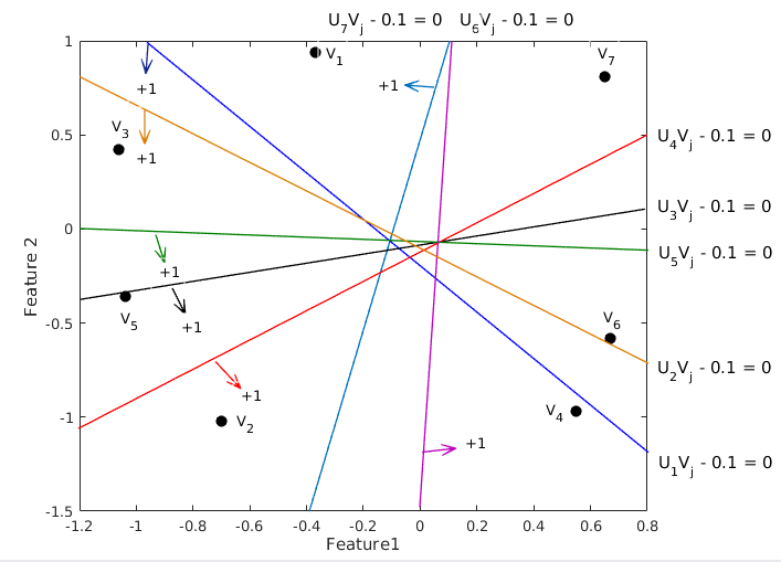
Figure 3.1: Geometrical interpretation of bi-level matrix factorization.

There are many matrix factorization algorithms for bi-level matrices which adopts the generic algorithm describe in Algorithm 1. These algorithms are designed based on the specification of the loss function and the regularization function. We adopt here a maximum-margin formulation as the guiding principle.

Loss functions in matrix factorization models are used to measure the discrepancy between the observed entry and the corresponding prediction. Furthermore, especially when predicting discrete values such as ratings, loss functions other then sum-squared loss are often more appropriate [rennie2005fast]. The trade-off between generalization loss and empirical loss has been prevailing since the advent of support vector machine (SVM). Maximum margin approach aims at providing higher generalization ability and avoiding overfitting. In this context, hinge loss function is the most preferred loss function and is defined as follows.

$$h(z)=\begin{cases}0,&\text{if z $\geq$ 1};\\ 1-z,&\text{otherwise},\end{cases}$$ (3.5)

where $z=y_{ij}(U_{i}V_{j}^{T})$. The hinge loss is illustrated in Figure 3.2.

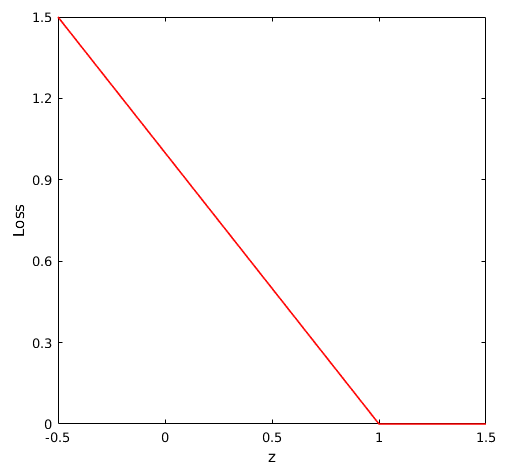
Figure 3.2: Loss function values for the hinge

The following real-valued prediction matrix is obtained from the latent factor matrices $U$ and $V$ (Table 3.4) corresponding to the matrix Y (Table 3.1).

Table 3.5: Real-valued prediction corresponding to bi-level matrix Y.

-0.24	0.95	0.46	0.14	0.84	-0.13	-0.81
-0.65	1.46	0.33	0.55	1.06	0.09	-1.23
-1.12	0.92	-0.74	1.21	0.11	0.81	-0.71
-1.02	0.42	-1.02	1.16	-0.35	0.91	-0.27
-0.96	1.06	-0.41	0.99	0.39	0.58	-0.85
-0.47	-0.80	-1.27	0.68	-1.23	0.81	0.75
0.61	0.56	1.26	-0.81	1.08	-0.87	-0.55

The hinge loss function values corresponding to the observed entries in $Y$ (Table 3.1) and the real-valued prediction (Table 3.5) is shown in Table 3.6.

Table 3.6: Hinge loss corresponding to observed entries in Y.

0	0.05	0	0	0.16	0	0
0.35	0	0.67	0.45	0	0	0.35
0	0.08	0.26	0	0	0.19	0
0	0.58	0	0	0.65	0.09	0
0.04	0	0.59	0.01	0.61	0	0.04
0	0.20	0	0.32	0	0.19	0
0.39	0.44	0	0.19	0	0	0.39

Hinge loss, $h(z)$ is non-differentiable at $z=1$ and is very sensitive to outliers as mentioned in [rennie2005fast]. Therefore an alternative called smooth hinge loss is proposed in [rennie2005loss] and can be defined as,

$$h(z)=\begin{cases}0,&\text{if z $\geq$ 1};\\ \frac{1}{2}(1-z)^{2},&\text{if $0<z<1$};\\ \frac{1}{2}-z,&\text{otherwise}.\end{cases}\\$$ (3.6)

The smooth hinge loss is illustrated in Figure 3.3.

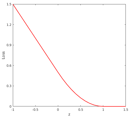
Figure 3.3: Loss function values for the smooth hinge

The smooth hinge loss function values corresponding to the observed entries in $Y$ (Table 3.1) and the real-valued prediction (Table 3.5) is shown in Table 3.7.

Table 3.7: Smooth hinge loss corresponding to observed entries in Y.

0	0	0	0	0.01	0	0
0.06	0	0.23	0.10	0	0	0.06
0	0	0.03	0	0	0.02	0
0	0.17	0	0	0.21	0	0
0	0	0.17	0	0.19	0	0
0	0.02	0	0.05	0	0.02	0
0.08	0.10	0	0.02	0	0	0.08

Figure 3.2 and 3.3 show the loss function values for the hinge and smooth hinge loss, respectively. It can be seen that the smooth hinge loss shares important similarities to the hinge loss and has a smooth transition between a zero slope and a constant negative slope. Table 3.6 and  3.7 show the hinge loss and smooth hinge loss function values corresponding to the observed entries in $Y$ (Table 3.1). It can also be seen that the smooth hinge is less sensitive to the outliers as compared to the hinge loss function. For example, the rating given by user $4$ for item $2$ is positive and the same reflect in the embedding (Figure 3.1). The loss incurred by hinge and smooth hinge are $0.58$ and $0.17$, respectively. Even though the point is embedded with margin the hinge loss function gives more reward to the model for the increase in objective value.

We reformulate P${}_{\mbox{$\pm{1}$}}$(Y) problem for the bi-level rating matrix as the following optimization problem.

$$\underset{U,V}{min}J(U,V)=\underset{(i,j)\in\Omega}{\Sigma}h\big{(}y_{ij}(U_{i}V_{j}^{T})\big{)}+\frac{\lambda}{2}(\|U\|^{2}_{F}+\|V\|^{2}_{F})$$ (3.7)

where $\|.\|_{F}$ is the Frobenius norm which is the same as defined in Chapter $2$, $\lambda>0$ is the regularization parameter and $h(\cdot)$ is the smooth hinge loss function as defined previously.

The gradients of the variables to be optimized are determined as follows. The gradient with respect to each element of $U$ is calculated as

$$\frac{\partial J}{\partial U_{ip}} =\sum_{j|(i,j)\in\Omega}\frac{\partial h\big{(}y_{ij}(U_{i}V_{j}^{T})\big{)}}{\partial U_{ip}}+\frac{\lambda}{2}\bigg{(}\frac{\partial\|U\|^{2}_{F}}{\partial U_{ip}}+\frac{\partial\|V\|^{2}_{F}}{\partial U_{ip}}\bigg{)}$$

$$=\sum_{j|(i,j)\in\Omega}y_{ij}h^{\prime}\big{(}y_{ij}(U_{i}V_{j}^{T})\big{)}\frac{\partial(U_{i}V_{j}^{T})}{\partial U_{ip}}+\lambda U_{ip}$$

$$=\sum_{j|(i,j)\in\Omega}y_{ij}h^{\prime}\big{(}y_{ij}(U_{i}V_{j}^{T})\big{)}V_{jp}+\lambda U_{ip}$$ (3.8)

Similarly, the gradient with respect to each element of $V$ is calculated as follows.

$$\frac{\partial J}{\partial V_{jq}} =\sum_{i|(i,j)\in\Omega}y_{ij}h^{\prime}(y_{ij}(U_{i}V_{j}^{T}))U_{iq}+\lambda V_{jq}$$ (3.9)

where $h^{\prime}(z)$ is defined as follows.

$$h^{\prime}(z)=\begin{cases}0,&\text{if z $\geq$ 1};\\ z-1,&\text{if $0<z<1$};\\ -1,&\text{otherwise}.\end{cases}$$ (3.10)

Algorithm 2 outlines the main flow of the bi-level maximum margin matrix factorization (BMMMF).

input : Bi-level Rating Matrix: $Y$, Number of Latent Factors: $d$, Regularization   Parameter: $\lambda$

output : Factor Matrices: $U$ and $V$

$t\leftarrow 0$;

Initialize: $U^{t}$, $V^{t}$;

while Stopping criteria met do

       $\frac{\partial J}{\partial U^{t}_{ip}}\leftarrow\sum_{j|(i,j)\in\Omega}y_{ij}h^{\prime}(y_{ij}(U_{i}^{t}V_{j}^{t^{T}}))V_{jp}^{t}+\lambda U_{ip}^{t}$ ;

       $\frac{\partial J}{\partial V^{t}_{jq}}\leftarrow\sum_{i|(i,j)\in\Omega}y_{ij}h^{\prime}(y_{ij}(U_{i}^{t}V_{j}^{t^{T}}))U_{iq}^{t}+\lambda V_{jq}^{t}$;

       $t\leftarrow t+1$;

       $U_{ip}^{t+1}\leftarrow U_{ip}^{t}-c\frac{\partial J}{\partial U_{ip}^{t}}$;

       $V_{jq}^{t+1}\leftarrow V_{jq}^{t}-c\frac{\partial J}{\partial V_{jq}^{t}}$;

      

end Let $U$ and $V$ are the factor matrices obtained after convergence;

return $U$ and $V$;

Algorithm 2 BMMMF ($Y$, $d$, $\lambda$)

We also show the behaviour of $J$ (Equation 3.7). We plot the value of $J$ obtained in every iteration for the same $Y$ (Table 3.1) starting from different initial points. It can be seen from Figure 3.4 that $J$ is having asymptotic convergence.

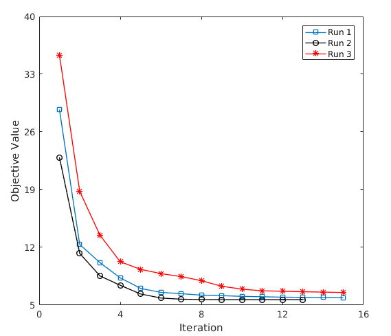
Figure 3.4: Convergence graph of BMMMF with different initial points

3.3   Multi-level MMMF

As discussed in the previous chapter, MMMF [srebro2004maximum] and subsequently, Fast MMMF [rennie2005fast] are proposed primarily for collaborative filtering with ordinal rating matrix when user-preferences are not in the form of like/ dislike but are values in a discrete range. The matrix completion of ordinal rating matrix is concerned with the following problem.

Problem P${}_{\mbox{ord}}$(Y): Let $Y$ be a $N\times M$ partially observed user-item rating matrix and $\Omega$ is the set of observed entries. For each $(i,j)\in\Omega$, the entry $y_{ij}\in\{1,2,\dots,R\}$ defines the preference of the $i$th user for the $j$th item. For each $(i,j)\notin\Omega$, $y_{ij}=0$ indicates that the preference of $i$th user for $j$th item is not available. Given a partially observed rating matrix $Y\in\mathbb{R}^{N\times M}$, the goal is to predict $y_{ij}$ for $(i,j)\notin\Omega$.

Need for multiple thresholds: Unlike P${}_{\mbox{$\pm{1}$}}$(Y), P${}_{\mbox{ord}}$(Y) has domain of $y_{ij}$ with more than two values. When the domain has two values, P${}_{\mbox{ord}}$(Y) is equivalent to P${}_{\mbox{$\pm{1}$}}$(Y). Continuing our discussion on geometrical interpretation of P${}_{\mbox{$\pm{1}$}}$(Y), the likes $(+1)$ and dislikes $(-1)$ of user $i$ are separated with both sides of the hyperplane defined by $U_{i}$. The same concept when extended to P${}_{\mbox{ord}}$(Y), it is necessary to define threshold values $\{\theta_{1},\dots,\theta_{R-1}\}$ such that the region between two parallel hyperplanes defined by the same $U_{i}$ with different threshold $\theta_{q-1}$ and $\theta_{q}$ corresponds to the rating $q$. Thus, in P${}_{\mbox{ord}}$(Y), in addition to learning the latent factor matrices $U$ and $V$ it is also needed to learn the thresholds $\theta$’s. There may be a debate on the number of $\theta$’s needed, but following the original proposal of MMMF [rennie2005fast], we follow $R-1$ thresholds for each user and hence there are $n(R-1)$ thresholds.

There are different approaches for constructing a loss function based on a set of thresholds such as immediate-threshold and all-threshold [rennie2005loss]. For each observed entry and the corresponding prediction pair $(y_{ij},U_{i}V_{j}^{T})$, the immediate-threshold based approach calculates the loss as sum of immediate-threshold violation which is $\ell(U_{i}V_{j}^{T}-\theta_{i,y_{ij}-1})~{}+~{}\ell(\theta_{i,y_{ij}}-U_{i}V_{j}^{T})$. On the other hand, all-threshold loss is calculated as the sum of loss for all thresholds which is the cost of crossing multiple rating-boundaries and is defined as follows.

$$\ell(U_{i}V_{j}^{T},y_{ij})=\sum_{r=1}^{y_{ij}-1}{\ell(U_{i}V_{j}^{T}-\theta_{i,r})}+\sum_{r=y_{ij}}^{R-1}{\ell(\theta_{i,r}-U_{i}V_{j}^{T})}$$ (3.11)

Using the $R-1$ thresholds $\theta$’s, MMMF extended the hinge loss function meant for binary classification to ordinal settings. The difference between immediate-threshold and all-threshold hinge is illustrated with the help of the following example. Let us consider the partially observed ordinal rating matrix $Y$ with $R=5$, the learnt factor matrices $U$, $V$ and the set of thresholds $\theta$’s for each user (Table 3.12).

Table 3.8: Runnning example.

1 2 4 3 5 2 1 4 3 0 0 4 5 3 2 4 1 1 3 2 4 3 5 5 2 0 2 3 1 4 5 0 1 2 3 1 4 3 5 2 2 5 3 4 2 4 0 3 1 1 0 1 5 3 1 5 3 2 4 4 4 2 5 1 4 3 2 5 0 3 2 2 3 1 3 4 5 0 5 4 5 4 5 2 3 1 4 0 1 2 3 0 4 5 1 2 1 5 3 4 () Y 0.22 -0.12 0.90 0.05 1.45 0.31 -1.52 0.04 0.94 1.06 1.09 -1.45 0.10 0.14 -0.60 -1.65 -0.24 0.71 0.48 0.59 () U -0.79 1.01 0.10 1.21 1.51 -0.32 0.76 0.63 -0.53 0.24 1.45 -0.79 -0.98 -0.74 -0.17 0.72 -0.72 -1.32 0.39 -0.63 () V -0.61 -0.18 0.51 1.21 -0.74 0.09 0.69 1.41 -1.42 -0.65 0.28 0.91 -1.35 -0.25 0.74 0.96 -0.50 0.25 0.77 1.44 -1.08 -0.60 0.56 1.51 -1.10 -0.24 0.34 0.62 -1.41 -0.62 0.13 0.99 -0.73 -0.24 0.02 0.83 -0.73 -0.51 0.09 0.90 () $\theta$’s

The following real-valued prediction matrix is obtained from the above latent factor matrices $U$ and $V$ corresponding to the matrix $Y$.

Table 3.13: Real-valued prediction corresponding to ordinal rating matrix $Y$.

-0.30 -0.12 0.37 0.09 -0.15 0.41 -0.13 -0.12 0.00 0.16 -0.66 0.15 1.34 0.72 -0.47 1.27 -0.92 -0.12 -0.71 0.32 -0.83 0.52 2.09 1.30 -0.69 1.86 -1.65 -0.02 -1.45 0.37 1.24 -0.10 -2.31 -1.13 0.82 -2.24 1.46 0.29 1.04 -0.62 0.33 1.38 1.08 1.38 -0.24 0.53 -1.71 0.60 -2.08 -0.30 -2.33 -1.65 2.11 -0.09 -0.93 2.73 0.00 -1.23 1.13 1.34 0.06 0.18 0.11 0.16 -0.02 0.03 -0.20 0.08 -0.26 -0.05 -1.19 -2.06 -0.38 -1.50 -0.08 0.43 1.81 -1.09 2.61 0.81 0.91 0.84 -0.59 0.26 0.30 -0.91 -0.29 0.55 -0.76 -0.54 0.22 0.76 0.54 0.74 -0.11 0.23 -0.91 0.34 -1.12 -0.18

One can see that the entry $y_{13}$ is observed as $4$ and the corresponding real-valued prediction is $0.37$. When immediate-threshold hinge is the loss measure, the overall loss is calculated as follows.

$$h(y_{13},U_{1}V_{3}^{T}) =h(U_{1}V_{3}^{T}-\theta_{i,3})+h(\theta_{i,4}-U_{1}V_{3}^{T})$$

$$=h(0.37-0.51)+h(1.21-0.37)$$

$$=h(-0.14)+h(0.84)$$

$$=0.65$$

where $h(\cdot)$ is the smooth hinge loss function as defined previously. For the same example, the overall loss with all-threshold hinge function is calculated as follows.

$$h(y_{13},U_{1}V_{3}^{T}) =h(U_{1}V_{3}^{T}-\theta_{i,1})+h(U_{1}V_{3}^{T}-\theta_{i,2})+h(U_{1}V_{3}^{T}-\theta_{i,3})+h(\theta_{i,4}-U_{1}V_{3}^{T})$$

$$=h(0.37+0.61)+h(0.37+0.18))+h(0.37-0.51)+h(1.21-0.37)$$

$$=h(0.98)+h(0.55)+h(-0.14)+h(0.84)$$

$$=0.75$$

Continuing our discussion on geometrical interpretation, immediate-threshold loss tries to embed the point $V_{3}$ into the region defined by the parallel hyperplanes $(U_{1},\theta_{i,3})$ and $(U_{1},\theta_{1,4})$ which basically mean that $U_{1}V_{3}^{T}-\theta_{1,3}>0$ and $U_{1}V_{3}^{T}-\theta_{1,4}<0$. The all-threshold hinge function not only tries to embed the points rated as $r$ into the region defined by $(U_{i},\theta_{r-1})$ and $(U_{i},\theta_{r})$ but also consider the position of the points with respect to other hyperplanes. It is also desirable that every point $V_{j}$ rated by user $i$ should satisfy the condition $U_{i}V_{j}^{T}-\theta_{i,r-1}>0$ for $r<y_{ij}$ and $U_{i}V_{j}^{T}-\theta_{i,r}<0$ for $r\geq y_{ij}$.

In MMMF [rennie2005fast], each hyperplane acts as a maximum-margin separator which is ensured by considering smooth hinge as the loss function (all-threshold hinge). The resulting optimization problem for P${}_{\mbox{ord}}$(Y) is

$$\underset{U,V}{min}\;J(U,V,\theta)\sum_{(i,j)\in\Omega}{\bigg{(}\sum_{r=1}^{y_{ij}-1}{h(U_{i}V_{j}^{T}-\theta_{i,r})}+\sum_{r=y_{ij}}^{R-1}{h(\theta_{i,r}-U_{i}V_{j}^{T})}\bigg{)}}+\frac{\lambda}{2}(\|U\|^{2}_{F}+\|V\|^{2}_{F})$$ (3.12)

where $\|.\|_{F}$ is the Frobenius norm, $\lambda>0$ is the regularization parameter, $\Omega$ is the set of observed entries, $h(z)$ is the smooth hinge loss as defined previously and $\theta_{i,r}$ is the threshold for rank $r$ of user $i$. The equation given above can be rewritten as follows.

$$\underset{U,V}{min}\;J(U,V,\theta)\;\sum_{r=1}^{R-1}{\sum_{(i,j)\in\Omega}h\big{(}T_{ij}^{r}(\theta_{i,r}-U_{i}V_{j}^{T}))}+\frac{\lambda}{2}(\|U\|^{2}_{F}+\|V\|^{2}_{F})$$ (3.13)

where $T$ is defined as

$$T_{ij}^{r}=\begin{cases}+1,&\text{if r $\geq$ $y_{ij}$;}\\ -1,&\text{if r $<$ $y_{ij}$.}\end{cases}$$

The gradients of the variables to be optimized are determined as follows. The gradient with respect to each element of $U$ is calculated as follows.

$$\frac{\partial J}{\partial U_{ip}} =\sum_{r=1}^{R-1}{\sum_{j|(i,j)\in\Omega}{\frac{\partial h\big{(}T_{ij}^{r}(\theta_{i,r}-U_{i}V_{j}^{T})\big{)}}{\partial U_{ip}}}}+\frac{\lambda}{2}\bigg{(}\frac{\partial\|U\|^{2}_{F}}{\partial U_{ip}}+\frac{\partial\|V\|^{2}_{F}}{\partial U_{ip}}\bigg{)}$$

$$=\sum_{r=1}^{R-1}{\sum_{j|(i,j)\in\Omega}{T_{ij}^{r}h^{\prime}\big{(}T_{ij}^{r}(\theta_{i,r}-U_{i}V_{j}^{T})\big{)}\frac{\partial(\theta_{i,r}-U_{i}V_{j}^{T})}{\partial U_{ip}}}}+\lambda U_{ip}$$

$$=\lambda U_{ip}-\sum_{r=1}^{R-1}{\sum_{j|(i,j)\in\Omega}{T_{ij}^{r}h^{\prime}\big{(}T_{ij}^{r}(\theta_{i,r}-U_{i}V_{j}^{T})\big{)}V_{jp}}}$$ (3.14)

where $h^{\prime}(\cdot)$ is the same as defined previously. Similarly, the gradients with respect to each element of $V$ is calculated as

$$\frac{\partial J}{\partial V_{jq}} =\lambda V_{jq}-\sum_{r=1}^{R-1}{\sum_{i|(i,j)\in\Omega}{T_{ij}^{r}h^{\prime}\big{(}T_{ij}^{r}(\theta_{i,r}-U_{i}V_{j}^{T})\big{)}U_{iq}}}$$ (3.15)

and the gradient with respect to each $\theta_{i,r}$ is determined as follows.

$$\frac{\partial J}{\partial\theta_{i,r}} =\sum_{j|(i,j)\in\Omega}{\frac{\partial h\big{(}T_{ij}^{r}(\theta_{i,r}-U_{i}V_{j}^{T})\big{)}}{\partial\theta_{i,r}}}+\frac{\lambda}{2}\bigg{(}\frac{\partial\|U\|^{2}_{F}}{\partial\theta_{i,r}}+\frac{\partial\|V\|^{2}_{F}}{\partial\theta_{i,r}}\bigg{)}$$

$$=\sum_{j|(i,j)\in\Omega}{T_{ij}^{r}h^{\prime}\big{(}T_{ij}^{r}(\theta_{i,r}-U_{i}V_{j}^{T})\big{)}\frac{\partial(\theta_{i,r}-U_{i}V_{j}^{T})}{\partial\theta_{i,r}}}$$

$$=\sum_{j|(i,j)\in\Omega}{T_{ij}^{r}h^{\prime}\big{(}T_{ij}^{r}(\theta_{i,r}-U_{i}V_{j}^{T})\big{)}}$$ (3.16)

Once $U$, $V$ and $\theta$’s are computed, the matrix completion process is accomplished as follows.

$$\hat{y}_{ij}=\begin{cases}r,&\text{if $(i,j)\notin\Omega\wedge(\theta_{i,r}\leq x_{ij}\leq\theta_{i,r+1})\wedge(0\leq r\leq R-1)$};\\ y_{ij},&\text{if $(i,j)\in\Omega$},\end{cases}$$

where, $\hat{y}_{ij}$ is the prediction for item $j$ by user $i$. For simplicity of notation, we assume $\theta_{i,0}=-\infty$ and $\theta_{i,R}=+\infty$ for each user $i$.

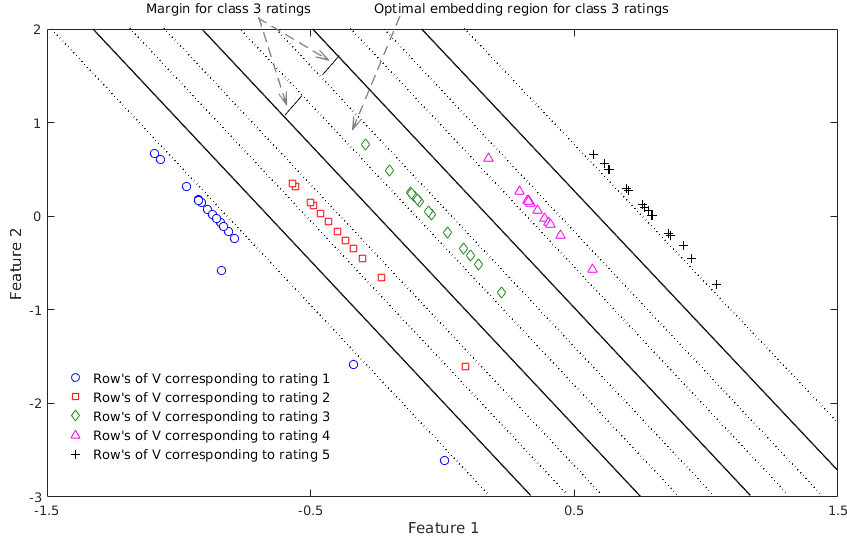
Figure 3.5: Classification by MMMF for the $i$th user

The objective of MMMF is to learn the embedding of items as points, users as hyperplanes and ratings as thresholds such that the points fall as correctly as possible into regions with the margin of ratings defined by the decision hyperplane $(U_{j},\theta_{j,r})$. We illustrate this concept by taking a synthetic dataset of size $5\times 1000$ with $10\%$ of observed entries. The number of ordinal ratings is $5$ and $d=2$. Figure 3.5 gives the decision hyperplane for a user and embedding of points corresponding to the items. Since $R=5$, there are $4$ hyperplanes that subdivide the entire space into $5$ regions corresponding to $5$ ratings. The data so chosen is balanced in the sense that the number of items for each rating is uniform. From the figure, it is clear that the embedding is learnt perfectly and the points corresponding to the items fall in the region of respective ratings with the margin. The margin is also shown in the figure by drawing parallel lines artifically. Thus, one can see that the embedding is achieved with true sense of maximum-margin. However, this is not so for all cases. It is observed through several experiments that the margin for the parallel lines is not the same and these hyperplanes separate classes with unequal margin with bias toward classes with sparse training samples. When the data is balanced, as in the previous case (Figure 3.5), the unequal margin phenomenon is not evident. In another synthetic example of size $5\times 1000$ with $20\%$ of observed entries, $R=5$, $d=2$ and where the data is not balanced the inequalities in the margin size is evident. This is depicted in Figure 3.6. In this example the observed entries for rating $2,3$ and $4$ are substantially less than those for ratings $1$ and $5$. The observed entries for rating $3$ is substantially less than the observed entries for ratings $2$ and $4$. When the points are embedded in two dimensional plane the parallel separating line corresponding to different thresholds for a given user have different margins and this is depicted in Figure 3.6. One can see that the hyperplanes tend to come closer towards the ratings with sparse samples. The hyperplane separating regions $4$ and region $5$ is not giving sufficient margin for rating $4$ but overfits rating $5$. The hyperplane separating regions $3$ and $4$ have unequal margin on both sides. So as a conclusion, it is observed that the proposed MMMF [rennie2005fast] is not truly handling margin maximization for predictions of ratings.

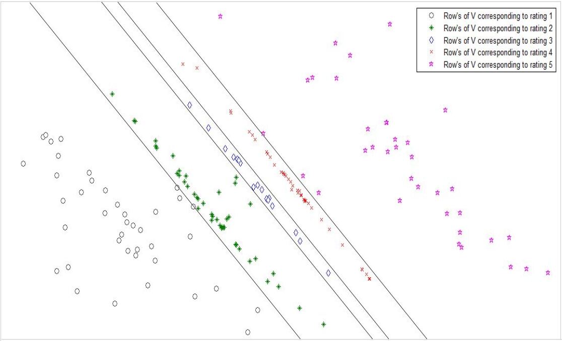
Figure 3.6: Classification by MMMF for $i$th user

We also show the behaviour of $J$ defined in Equation 3.13. We plot the value of $J$ obtained in every iteration for the same $Y$ (Table 3.12) starting from different initial points. It can be seen from Figure 3.7 that $J$ is having asymptotic convergence.

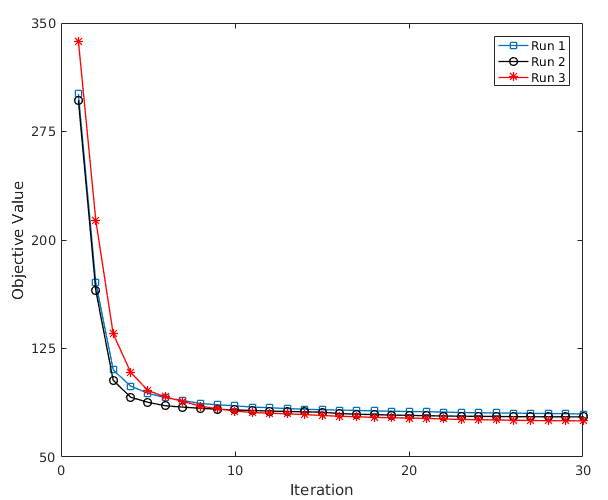
Figure 3.7: Convergence graph of MMMF with different initial points

For ordinal ratings with discrete values such as $1$-$5$ stars, it is necessary to think of a sort of multiclass separation such that items are classified based on ratings which take on values from a finite discrete set. MMMF [rennie2005fast] follows the principle of single machine extension and handles ordinal rating matrix factorization by proposing a multi-class extension of the hinge loss function.

3.4   HMF- The Proposed Method

In this section, we describe the proposed method, termed as HMF (Hierarchical Matrix Factorization). As discussed in Section 3.1, the proposed method draws motivation from research on multi-class classification. There are two major approaches for addressing multi-class classification problems namely embedded techniques [weston1999support, lee2004multicategory, crammer2001algorithmic, blondel2013block] and combinational technique [hsu2002comparison, rifkin2004defense, bahlmann2002online]. The first approach explicitly formulate the multi-class problem directly. The second approach (combinational technique) is to decompose the multi-class problem to multiple independent binary classification problems. In (MMMF) [rennie2005fast], an embedded approach is proposed to address the P${}_{\mbox{ord}}$(Y) problem. The authors has extended hinge loss defined for binary-level to multi-level cases. As discussed in Section 3.3, the extension of hinge-loss to multi-level does not preserve the property of maximum margin and also impose the parallel constraints on decision hyperplane. Our goal is to examine a solution to the P${}_{\mbox{ord}}$(Y) problem by constructing a hierarchy of bi-level MMMF using the principle of combinational approach. We believe that by following the principle of combinational approach the maximum margin advantage of bi-level matrix factorization can be retained and the parallel constraints on the decision hyperplane can also be relaxed.

As discussed previously, HMF is a stage-wise matrix completion technique that makes use of several bi-level MMMFs in a hierarchical fashion. At every stage $q$ of HMF, the original problem P${}_{\mbox{ord}}$(Y) is converted to P${}_{\mbox{$\pm{1}$}}$(Y) and solved using the method described in Section 3.2. The output at stage $q$ is the learnt latent factor matrices $U^{q}$ and $V^{q}$. The so computed latent factors $U^{q}$ and $V^{q}$ are used to predict the entries of the matrix of a specific ordinal value $q$. In other words, at Stage $q$ , HMF attempts to complete only those unobserved entries of the rating matrix where the rating $q$ is predicted. Thus for a $R$ -level ordinal rating matrix, we use $R-1$ stages. The method of conversion from P${}_{\mbox{ord}}$(Y) to P${}_{\mbox{$\pm{1}$}}$(Y) at stage $q$ is discussed below.

Conversion of P${}_{\mbox{ord}}$(Y) to P${}_{\mbox{$\pm{1}$}}$(Y): At every stage $q$ of HMF, a BMMMF is employed and for this purpose, the P${}_{\mbox{ord}}$(Y) is converted to P${}_{\mbox{$\pm{1}$}}$(Y) problem as follows.

$$y_{ij}^{q}=\begin{cases}-1,&\text{if $(i,j)\in\Omega\wedge y_{ij}\leq q$};\\ +1,&\text{if $(i,j)\in\Omega\wedge y_{ij}>q$};\\ 0,&\text{if $(i,j)\notin\Omega$.}\end{cases}$$ (3.17)

This conversion states that any rating above $q$ is treated as $likes$ and below or equal to $q$ is treated as $dislike$.

The outcome of BMMMF at stage $q$ are the factor matrices $U^{q}$ and $V^{q}$ approximating $Y^{q}$. Let $\hat{Y}^{q}$ be the bi-level prediction matrix obtained from the factor matrices $U^{q}$ and $V^{q}$ and $\Omega^{q}$ is the index set corresponding to the $-1$ entries in $\hat{Y}^{q}$. For simplicity of notation, we assume $\Omega^{0}$ is empty. The entries in ordinal rating prediction matrix $\hat{Y}$ are predicted as $q$ based on the following rule.

$$\hat{y}_{ij}=\begin{cases}q&\text{if $(i,j)\notin{(\Omega^{0}\cup\Omega^{1}\dots\cup\Omega^{q-1})}\wedge(\Omega^{q}=-1)$}\\ y_{ij}&\text{if $(i,j)\in\Omega$ }\end{cases}$$ (3.18)

At the last stage, stage $R-1$, after employing the above rule to predict entries with values $R-1$, we complete the matrix by assigning $R$ for all remaining unobserved entries.

Algorithm 3 outlines the main flow of the proposed method HMF for the ordinal rating matrix completion problem.

input : Ordinal Rating Matrix: $Y$, Maximum Rating: $R$, Number of Latent   Factors: $d$, Threshold: $\theta$, Regularization Parameters: $\{\lambda_{1},\dots,\lambda_{R-1}\}$

output : $\hat{Y}$

Initialize: $\hat{Y}\leftarrow 0$;

for $q=~{}1~{}to~{}R-1$ do

       $Y^{q}\leftarrow 0$;

       for $(i,j)\in\Omega$ do

             if $y_{ij}\leq q$ then

                   $y_{ij}^{q}=-1$;

            else

                   $y_{ij}^{q}=+1$;

            end

      end ($U^{q}$, $V^{q}$) $\leftarrow$ BMMMF ($Y^{q}$, $d$, $\lambda_{q}$);

       for ever user-item pair $(i,j)$ do

             if $U_{i}^{q}V_{j}^{q^{T}}<\theta$ then

                   $\hat{y}_{ij}^{q}$ = -1;

            else

                   $\hat{y}_{ij}^{q}$ = +1;

            end

      end for ever user-item pair $(i,j)$ do

             if $\big{(}(i,j)\notin\Omega\wedge\hat{y}_{ij}^{q}=-1\big{)}\vee y_{ij}=q$ then

                  $\hat{y}_{ij}\leftarrow q$

            end

      end

end $\hat{y}_{ij}\leftarrow R$,  if $\hat{y}_{ij}=0$, $\forall(i,j)\notin\Omega$ ;

return $\hat{Y}$;

Algorithm 3 HMF ($Y$, $R$, $d$, $\theta$, $\lambda$)

We illustrate the working of HMF using a toy example. Let us consider the following partially observed ordinal rating matrix $Y$ of size $5\times 7$ with $5$ levels.

Table 3.14: Ordinal rating matrix Y

3	0	0	5	2	0	0
5	4	0	1	5	3	4
1	0	4	0	3	1	0
5	4	0	0	0	0	1
0	3	2	0	5	2	0

For notational convenience, we use $ij$ to denote $(i,j)$. The set of observed entries $\Omega=\{11,14,15,21,22,24,25,26,27,31,33,35,36,41,42,47,52,53,55,56\}$. For each of the $4$ stages, the original $5$-level rating matrix $Y$ is converted to a bi-level ($\pm 1$) matrix. Taking $d=2$, we employed bi-level MMMF to get factor matrix pairs $(U^{q},V^{q})$ for each stage $q$ independently. At stage $1$, the bi-level matrix $Y^{1}$ obtained from $Y$, the learnt latent factor matrices $U^{1}$ and $V^{1}$ and the corresponding bi-level prediction $\hat{Y}^{1}$ is shown in Table 3.19.

Table 3.15: Runnning example.

1 0 0 1 1 0 0 1 1 0 -1 1 1 1 -1 0 1 0 1 -1 0 1 1 0 0 0 0 -1 0 1 1 0 1 1 0 () $Y^{1}$ -0.48 -0.54 0.12 -1.09 0.98 -0.13 -0.77 -0.29 -0.01 -0.94 () $U^{1}$ -0.70 -0.63 -0.36 -0.72 0.47 -0.53 -0.51 0.25 0.28 -0.80 -0.52 -0.66 0.58 -0.37 () $V^{1}$ 1 1 1 1 1 1 -1 1 1 1 -1 1 1 1 -1 -1 1 -1 1 -1 1 1 1 -1 1 1 1 -1 1 1 1 -1 1 1 1 () $\hat{Y}^{1}$

At stage $1$, the set of entries $\Omega^{1}=\{17,24,31,32,34,36,43,47,54\}$ are predicted as $-1$. The set of entries $\Omega^{1}\setminus\Omega$ i.e., $\{17,32,34,43,54\}$ and the set of entries where $1$ are observed now contains rating $1$ in the partially complete prediction matrix $\hat{Y}$ (Table 3.20).

Table 3.20: Partially complete matrix after stage 1

0	0	0	0	0	0	1
0	0	0	1	0	0	0
1	1	0	1	0	1	0
0	0	1	0	0	0	1
0	0	0	1	0	0	0

Similarly, at stage $2$, the original matrix is mapped to bi-level matrix $Y^{2}$. The bi-level MMMF is employed on $Y^{2}$ to get the factor matrices $U^{2}$ and $V^{2}$. The factor matrices and the corresponding bi-level prediction $\hat{Y}^{2}$ is shown in the Table 3.25.

Table 3.21: Runnning example.

1 0 0 1 -1 0 0 1 1 0 -1 1 1 1 -1 0 1 0 1 -1 0 1 1 0 0 0 0 -1 0 1 -1 0 1 -1 0 () $Y^{2}$ -0.69 -0.47 -0.43 1.06 0.92 0.01 -0.79 0.05 0.24 0.86 () $U^{2}$ -0.89 0.21 -0.43 0.64 0.42 -0.54 -0.21 -0.67 0.53 0.76 -0.76 0.01 0.35 0.56 () $V^{2}$ 1 -1 -1 1 -1 1 -1 1 1 -1 -1 1 1 1 -1 -1 1 -1 1 -1 1 1 1 -1 1 -1 1 -1 -1 1 -1 -1 1 -1 1 () $\hat{Y}^{2}$

As discussed previously, at any stage $q$, the candidate set of entries for prediction will exclude the set of observed entries and the set of entries predicted before stage $q$. At stage $2$, the set of entries $\Omega^{2}=\{12,13,15,17,23,24,31,32,34,36,43,45,47,51,53,\linebreak 54,56\}$ are predicted as $-1$. The set of entries $\Omega^{2}\setminus\{\Omega^{1}\cup\Omega\}$ i.e., $\{12,13,23,45,51\}$ along with the entries where $2$ are observed now contains rating $2$ in the partially complete prediction matrix $\hat{Y}$ (Table 3.26).

Table 3.26: Partially complete matrix after stage 2

0	2	2	0	2	0	1
0	0	2	1	0	0	0
1	1	0	1	0	1	0
0	0	1	0	2	0	1
2	0	2	1	0	2	0

The bi-level mapping $Y^{3}$, the latent factor matrices $U^{3}$, $V^{3}$ and the corresponding bi-level prediction $\hat{Y}^{3}$ obtained at stage $3$ is shown in able 3.31.

Table 3.27: Runnning example.

-1 0 0 1 -1 0 0 1 1 0 -1 1 -1 1 -1 0 1 0 -1 -1 0 1 1 0 0 0 0 -1 0 -1 -1 0 1 -1 0 () $Y^{3}$ -0.42 0.70 0.26 -1.05 -0.80 0.44 0.84 0.08 -0.05 -0.81 () $U^{3}$ 0.72 -0.54 0.80 -0.12 -0.18 0.68 -0.26 0.62 0.26 -0.83 0.59 0.52 -0.39 -0.57 () $V^{3}$ -1 -1 1 1 -1 1 -1 1 1 -1 -1 1 -1 1 -1 -1 1 1 -1 -1 1 1 1 -1 -1 1 1 -1 1 1 -1 -1 1 -1 1 () $\hat{Y}^{3}$

It can be seen from Table 3.31 that the entries set $\Omega^{3}=\{11,12,14,15,23,25,31,32,\\ 35,36,43,44,46,53,54,56\}$ are predicted as $-1$. The set of entries $\Omega^{3}\setminus\{\Omega^{1}\cup\Omega^{2}\cup\Omega\}$ i.e., $\{44\}$ and the set of entries where $3$ are observed now is fixed to $3$ in $\hat{Y}$ (Table 3.32).

Table 3.32: Partially complete matrix after stage 3

3	2	2	0	2	0	1
0	0	2	1	0	3	0
1	1	0	1	3	1	0
0	0	1	3	2	0	1
2	3	2	1	0	2	0

Similarly, at stage $4$, the observed matrix $Y$ is mapped to bi-level matrix $Y^{4}$. Table 3.37 shows the bi-level matrix $Y^{4}$, the factor matrix $U^{4}$, $V^{4}$ and the corresponding bi-level prediction matrix $\hat{Y}^{4}$ obtained at stage $4$.

Table 3.33: Runnning example.

-1 0 0 1 -1 0 0 1 -1 0 -1 1 -1 -1 -1 0 -1 0 -1 -1 0 1 -1 0 0 0 0 -1 0 -1 -1 0 1 -1 0 () $Y^{4}$ 0.76 0.28 -0.76 -0.73 0.81 -0.58 -0.71 -0.43 -0.43 -0.85 () $U^{4}$ -0.89 -0.15 0.54 0.55 -0.17 0.69 0.58 0.35 -0.86 -0.27 0.01 0.83 0.54 0.40 () $V^{4}$ -1 1 1 1 -1 1 1 1 -1 -1 -1 1 -1 -1 -1 1 -1 1 -1 -1 1 1 -1 -1 -1 1 -1 -1 1 -1 -1 -1 1 -1 -1 () $\hat{Y}^{4}$

The set of entries $\Omega^{4}=\{11,15,22,23,24,26,27,31,33,35,36,42,43,44,46,47,52,53\\ ,54,56,57\}$ are predicted as $-$ at stage $4$. The set of entries $\Omega^{4}\setminus\{\Omega^{1}\cup\Omega^{2}\cup\Omega^{3}\cup\Omega\}$ i.e., $\{46,57\}$ and the set of entries where $4$ are observed now contains rating $4$ in the partially complete prediction matrix $\hat{Y}$ (Table 3.38).

Table 3.38: Partially complete matrix after stage 4

3	2	2	0	2	0	1
0	4	2	1	0	3	4
1	1	4	1	3	1	0
0	4	1	3	2	4	1
2	3	2	1	0	2	4

After completion of stage $4$, the set of entries where $0$ is present in $\hat{Y}^{4}$ are filled with rating $5$. The resulting complete matrix is shown in Table 3.39.

Table 3.39: Complete matrix computed by HMF

3	2	2	5	2	5	1
5	4	2	1	5	3	4
1	1	4	1	3	1	5
5	4	1	3	2	4	1
2	3	2	1	5	2	4

For the example given in Table 3.14, the complete process of HMF is summarized in Figure 3.8.

Figure 3.8: Hierarchical matrix factorization